[go: up one dir, main page]

Article

Heavy Metal Groundwater Transport Mitigation from an Ore Enrichment Plant Tailing at Kazakhstan’s Balkhash Lake

1
Department of Hydrogeology, Engineering and Petroleum Geology, Satbayev University, Almaty 050000, Kazakhstan
2
Department of Chemical Engineering, Ariel University, Ariel 40700, Israel
3
Department of Environmental Research, Eastern R&D Center, Ariel University, Ariel 40700, Israel
4
Akhmedsafin Institute of Hydrogeology and Environmental Geoscience, Almaty 050000, Kazakhstan
*
Author to whom correspondence should be addressed.
Sustainability 2024, 16(16), 6816; https://doi.org/10.3390/su16166816
Submission received: 11 June 2024 / Revised: 2 August 2024 / Accepted: 5 August 2024 / Published: 8 August 2024
Figure 1
<p>The study site location map and the Balkhash Industrial Area aerial photo display industrial objects included in the model’s schematization where the orange line is an interface with water bodies, the purple line is the tailing storage interface, black lines are barriers, and green lines are drains. The figure was prepared by Corel Draw with a base experimental site image taken from Google Earth.</p> ">
Figure 2
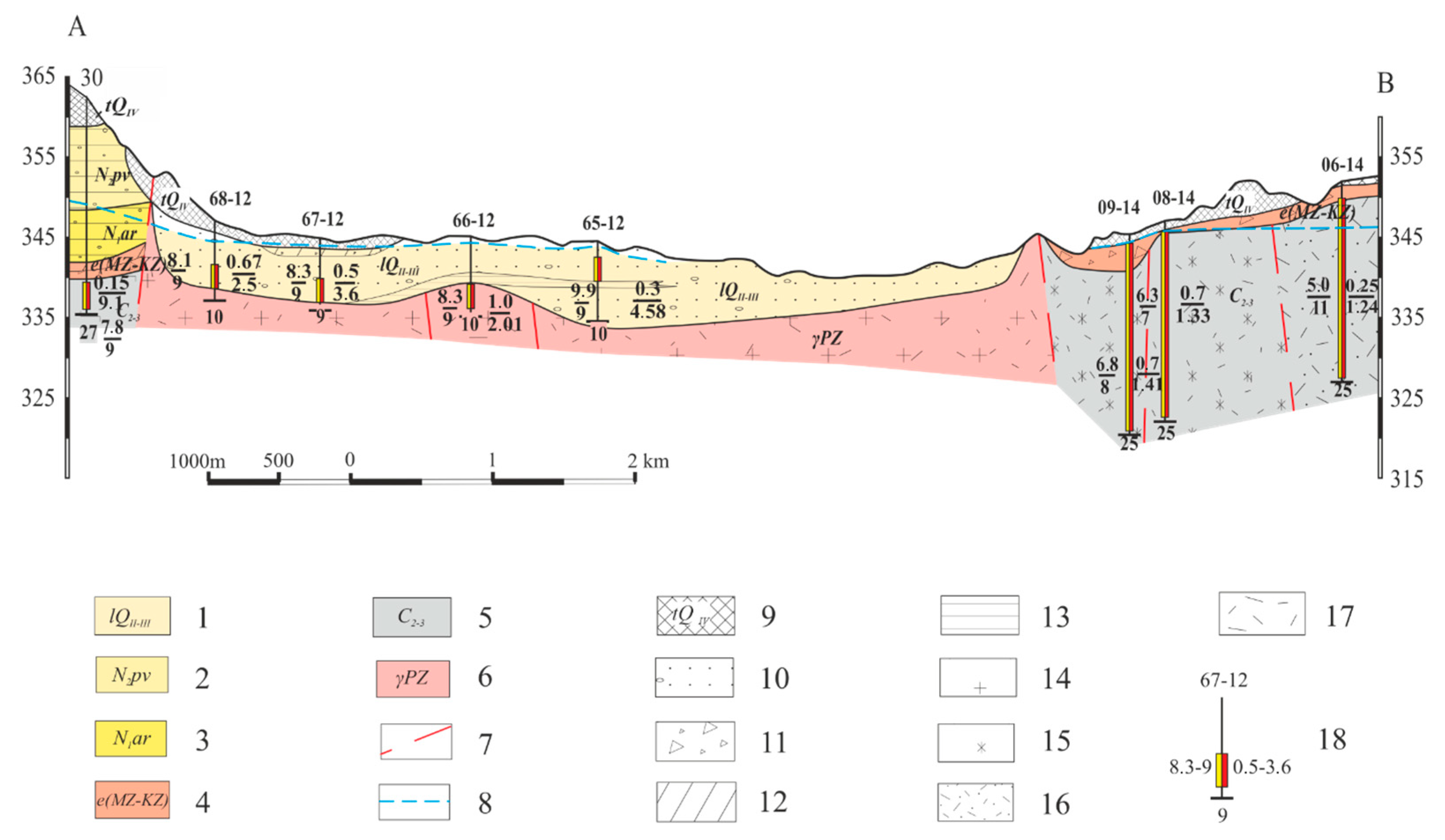
<p>Hydrogeological cross-section along lines A–B (<a href="#sustainability-16-06816-f001" class="html-fig">Figure 1</a>). 1—upper-middle Quaternary lacustrine aquifer; 2—Pliocene aquitard of Pavlodar formations; 3—Miocene aquitard of Argyn formations; 4—Meso-Cenozoic water-bearing formations; 5—Carboniferous aquifer; 6—Paleozoic zone of fractured intrusive rocks; 7—tectonic faults; 8—groundwater level; 9—upper Quaternary technogenic aquifer, bulk soil; 10—sands with gravel inclusions; 11—crushed stones; 12—loams; 13—clays; 14—granites; 15—syenite porphyries; 16—dacite porphyries; 17—fractured rock; 18—well. Numbers: on top—well number, bottom—well depth, m; on the left in the numerator—mineralization, g/L; in the denominator—temperature, °C; on the right: in the numerator—well flow rate, L/s; in the denominator—drawdown, m. Shading corresponds to the chemical composition of groundwater in the sampled interval with the predominance of chloride and sulfate anions.</p> ">
Figure 3
<p>The conceptual working process applied for the Balkhash Lake contamination risk assessment (<b>a</b>) and model application steps (<b>b</b>).</p> ">
Figure 4
<p>Model calibration results.</p> ">
Figure 5
<p>(<b>a</b>) Path lines of particles released from the source of pollution by the area tracked with MODPATH and (<b>b</b>) heavy metal spatial distribution in groundwater for ten years after contaminant release without a change in hydrogeological conditions (legend in <a href="#sustainability-16-06816-t001" class="html-table">Table 1</a>).</p> ">
Figure 6
<p>Spatial distribution of heavy metals in groundwater from 14 drainage wells drilled between the drainage channel and Lake Balkhash (<b>a</b>) and for the scenario of drilling ten drainage wells between the drainage channel and Lake Balkhash (<b>b</b>).</p> ">
Figure A1
<p>Spatial distribution of heavy metals in groundwater for the scenario of boundary construction between the drainage channel and Lake Balkhash.</p> ">
Figure A2
<p>Spatial distribution of heavy metals in groundwater for the scenario of drainage wells drilled between the tailings pond drainage channel and the lake.</p> ">
Figure A3
<p>Results of heavy metal concentration in groundwater monitoring wells over time.</p> ">
Figure A4
<p>Sampling points on a map of heavy metal halo distribution in groundwater at the time of sampling in 2020.</p> ">
Figure A5
<p>Calibration graph of the observed and calculated heavy metal concentrations at the sampling points.</p> ">
Figure A6
<p>Relative sensitivity coefficients concerning different input parameters for a ±50% change in each parameter.</p> ">
Versions Notes

Abstract

:
Sustainable potable groundwater supply is crucial for human development and the preservation of natural habitats. The largest endorheic inland lake in Kazakhstan, Balkhash Lake, is the main water resource for the arid southeastern part of the country. Several ore enrichment plants that are located along its shore have heavy metal pollution potential. The study area is located around a plant that has an evident anthropogenic impact on the Balkhash Lake aquatic ecological system, with ten known heavy metal toxic hotspots endangering fragile habitats, including some indigenous human communities. This study assessed the risk of heavy metal contamination from tailing dump operations, storage ponds, and related facilities and suggested management practices for preventing this risk. The coastal zone risk assessment analysis used an innovative integrated groundwater numerical flow and transport model that predicted the spread of groundwater contamination from tailing dump operations under several mitigation strategies. Heavy metal pollution prevention models included a no-action scenario, a filtration barrier construction scenario, and two scenarios involving the drilling of drainage wells between the pollution sources and the lake. The scenario assessment indicates that drilling ten drainage wells down to the bedrock between the existing drainage channel and the lake is the optimal engineering solution for confining pollution. Under these conditions, pollution from tailings will not reach Lake Balkhash during the forecast period. The methods and tools used in this study to enable mining activity without environmental implications for the region can be applied to sites with similar anthropogenic influences worldwide.

1. Introduction

Human and natural habitat sustainability is dependent on a clean water supply [1]. Heavy metals are nonbiodegradable pollutants with long cycle times that have been found to endanger endemic organisms and humans [2,3], making them a severe environmental problem in many parts of the world [4]. In China, lead, arsenic, and cadmium from industrial and stockpile origins were found to exceed the environmental standard concentrations in soils [5], rivers [6], and lakes [7]. The pollutant migration time from surface to groundwater was approximately 12 years [8], which can be considered a human health and environmental risk. Regression and principal component analyses in Tehran’s landfill indicated anthropogenic heavy metal accumulation with related toxic soil effects [9].
Surface water heavy metal concentration-based risk analysis has been performed in China [7,10], Mexico [11], Fiji [12], India [13,14], Kazakhstan [15], and other countries. Heavy metal behavior in groundwater is complicated and dependent on the water source, local lithology, and natural and technogenic biogeochemical processes [16]; population and economic growth have been found to intensify heavy metal contamination [17]. Heavy metal pollution occurs via several pathways, such as fertilizer and pesticide overuse, untreated industrial waste [18], solid waste dumping sites [19], and mine drainage [20]. In soils around mining tailing dams, the heavy metal contamination is usually significantly higher than the local background value, directly or indirectly contaminating the surrounding soil and posing a severe environmental threat [21].
Since the data are stochastic, nonlinear, nonstationary, and complex, no generalized ML model can handle all types of heavy metal migration and adsorption systems, and correct input parameter selection is essential to allow predictability [22].
Heavy metal and nutrient sources and their entry routes into Lake Balkhash were studied via distribution maps (cadmium, nickel, cobalt, lead, zinc, and copper) and nutrient reconstruction, which indicated that while Cu and Zn entered the water bodies mainly through agricultural wastewaters, Cd, Ni, Co, Pb, and, in part, Zn originated mainly from industrial and surface runoff [23]. A 20-year survey of ten trace elements revealed toxic element hotspots near industrial sites, such as smelters or mining and metallurgical complexes in surface waters (Cd and Pb), soil (As), and sediments (Cd and As), and less toxic elements, such as Cu, Zn, and Mn [24].
Heavy metal pollution of surface water is a common problem in Kazakhstan [25] and endangers the fragile regional ecosystem around its largest endorheic lake, the Balkhash (Figure 1) [26]. Agricultural pesticides have been found in the water supply and soils of several villages in the region [27], as have heavy metals in urban soils. Currently, human health and the ecosystem are endangered by industrial sources, such as zinc, cadmium, lead, copper and chromium polymetallic ore complexes [28]. Without corrective action, there may be devastating effects as a result of the anthropogenic pressure damage as seen at the Aral Sea and the Dead Sea inland lakes [29]. The Balkhash Enrichment Plant located on the lake’s shore results in heavy metal contamination, with cadmium and lead already posing severe risks [24,25].
Central Asia’s leading water and climate regulators are the Aral Sea and Balkhash Lake. As such, they were found to sustainably facilitate areas of ecological sources with dependent agricultural production systems. It is suggested that harm to these imperative ecological features might jeopardize human and natural habitats sustainability in Kazakhstan and all of Central Asia [30]. The primary objective of this study was to develop a heavy metal pollution expansion area prediction model that enables risk assessment of heavy metal contamination in Balkhash Lake due to the operation of industrial tailings systems, storage ponds, and related facilities. Our research focuses on whether it is possible to prevent further migration of heavy metals from the industrial zone to the lake and, if so, how. The research hypothesis was that at least one of the methods tested would successfully keep the pollution out of the lake.

2. Materials and Methods

2.1. Research Site Background and Geographical Framework

Balkhash Lake is the sink of a continental-type terminal basin located in the lowest part of the Balkhash depression at an altitude of 340 m. It is a long and narrow water body with at least 15,500 sq. km of water area. The lake’s catchment basin area is approximately 413,000 sq. km, including 353,000 sq. km (~85%) within Kazakhstan (Figure 1). The total watershed length is approximately 4000 km, and the active catchment area is approximately 135,000–170,000 sq. km, which is 33–41% of the total basin area. The lake surface area is between eight and nine times smaller than the active runoff area and approximately 27 times smaller than that of the whole basin [31,32]. Climate change in the region is manifested by general increasing temperatures and drying trends, resulting in earlier and shorter growing seasons [33] that require the allocation of additional water resources to agriculture [34]. The lake level varies from 343 m to 341 m, with a decrease of ~2 m between 1970 and 1984; at present, it has recovered to 343 m.
The Balkhash Industrial Area is located on the northwest coast of the lake and is adjacent to Torangalyk Bay (Figure 1). The Balkhash Enrichment Plant is the largest in the industrial area, with the main activity involving the enrichment of polymetallic ores and related manufacturing purposes. The Balkhash Enrichment Plant utilizes Vanyukov smelting furnaces to produce copper. The furnaces oxidize charge components with blast oxygen, thereby reducing the fuel component of the energy mix. Recovery boilers also utilize heat energy from copper smelting furnaces and converters. Most by-products and waste are recycled. The water is circulated in closed cycles, so industrial effluent into water bodies is minimal. If such discharges occur, the effluent may contain ions of metals such as Cu, Pb, Zn, Cd, Se, Mn, and As.
Furthermore, effluents may also exhibit increased acidity values due to the presence of sulfuric and (much less frequently and in much smaller volumes) hydrochloric and hydrofluoric (fluoric) acids [35]. The tailings storage facility is three kilometers from the main industrial area in an alluvial ravine–gully tailings dump. The enrichment plant tailings storage facility is a flat structure formed by embanking a part of the existing tailings storage area. It has an area of approximately 18.8 sq. km, with an adjacent tailings pond of approximately 14.03 sq. km. The tailings storage facility has an additional 25-year operation period up to a maximal water level of 374 m. The tailings storage facility drainage system includes two channels and pumping stations. The drainage channels run along the southern dam of the tailing’s storage facility and the evaporative pond dam. The channel is 8600 m long and passes through aeolian deposits and sandy to rocky soils (Figure 1).
Erosion–tectonic and denudation genesis of ridge–hilly relief is manifested by dome-shaped hills and ridges with lengths that do not exceed 1–2 km and widths ranging from 100 to 300 m, without a specific direction that is separated by a dense network of burrows. The domes have gentle slopes with elevations varying from 8–10 to 20–40 m. The accumulative delta gently descends to the Balkhash Lake through a 1–5 km wide swampy reed-covered coastline. Creeks across the coastline have a depth of up to three meters and a length of up to 25 m. The denudation plain has crusts up to a few meters wide and a pronounced thalweg [36].
The region’s stratigraphic section involves multiple folding and magmatic processes with Paleozoic rocks that are usually covered by loose Cenozoic sediments [32] with water-bearing horizons (Figure 2):
Bulk technogenic sediment (tQIV) debris flow formed paleosols comprising fine sands, sandy loams, and silts. During the first decade of the tailing operation, water was discharged directly into Torangalyk Bay. The boreholes drilled south of drainage channel No. 1 uncovered a 0.20 to 4.50 m thick sediment layer.
The upper-middle Quaternary lacustrine aquifer (lQII-III) occupies buried river valleys and numerous channels. This alluvial deposit horizon forms a continuous groundwater flow conduit with a phreatic water table. The aquifer has an average thickness of 9.9 m of loams and sandy loams ranging from 0.5 to 4.0 m, which represents the upper part of the section underlaid by alluvial sandy gravel and sandy pebbles with thin interlayers and clay lenses. The total gravel–sandy-pebble layer thickness varies from 4–5 m to 45–50 m. Around the lakeshore, groundwater is 2 to 3 m deep, but the average phreatic level is 6 to 8 m. The average flow rates are 20–26 L/s and the average hydraulic conductivity is 90–100 m/day. The groundwater mineralization varies from 0.5 to 1.0 g/L with an average of 0.7–0.8 g/L. The aquifer contains brackish water in the coastal zone with a 4.0–6.5 g/L salinity.
The Pavlodar Formation Pliocene aquitard and the Argyn Formation Miocene aquitard comprise clays that divide it into a series of water-bearing layers that, in some places, are hydraulically connected. The water-bearing layer thickness varies from 2 to 58 m. The lenses and clay interlayers are often marly and plastered, with thicknesses of 1 to 10 to 15 m. These layers, which are located closer to the lake, constitute an aquitard section of up to 20 m in thickness.
The Meso-Cenozoic aquitard prevails in the western part of the study area and is associated with clayey, sandy, and gravelly complexes, such as gravel-containing clays and gravel–sand fill layers. The layer thickness varies from a fraction of a meter to 12.2 m, with 1.5–2.5 m on average. The well productivity does not exceed 0.001–0.02 L/s of fresh and slightly brackish waters.
The Carboniferous aquifer (C2-3) consists of albitophyre, dacite porphyry, sandstone, siltstone, tuff sandstones, limestones, and conglomerate lenses. All the rocks have well-developed fracturing, but the cracks are often filled with clay weathering products or secondary quartz and calcite. The groundwater table is at a depth of 0.9–21.1 m and the active fractured zone thickness reaches 20–30 m. The wells are set in tectonically weakened zones with flow rates of 0.2–0.3 L/s and water level drawdown under pumping of 1.4–13.4 m. The hydraulic conductivity of the rock is low and varies from 0.1 to 3.8 m/day. The groundwater salinity ranges from 1.1 to 35.5 g/L but mostly ranges from 2 to 5 g/L. The predominant composition of groundwater is sulfate and sulfate–chloride components.
The Paleozoic water-bearing zone of fractured intrusive rock (γPz) granites are distributed in weathered and fractured blocks. In most parts, the cracks are filled with clayey weathering products or healed by secondary minerals. According to drilling data, the active fractured zone thickness is 10–30 m, which increases in the crushed rock zones up to 100 m or more. The hydraulic conductivity varies from 0.026 m/d for fractured rocks to 0.92–0.96 m/d for crushed zones and the water salinity ranges from 0.6 to 6.1 g/L.

2.2. Methodology

The ArcGIS 10.4 platform combines Copernicus satellite-based global land service data, a groundwater modeling system (GMS), field experiments and monitoring data for data processing and visualization. Orbital remote sensing was utilized to supply a digital terrain model (DTM) that improved the DEM and provided land cover and land use mapping. The information was converted into special data formats used for GMS numerical groundwater model construction [37]. Integrated laboratory tests and HYDRUS-1D modeling were used to simulate lead immobilization in contaminated soil and the underlying groundwater [38]. Pollutant migration from an abandoned tannery to soil and groundwater was assessed via ion balance simulation software (Visual MINTEQ v 3.1) and groundwater flow and solute transport software (Visual MODFLOW, version 4.1, MT3DMS, version 1.0.1) [39]. Based on the Visual MINTEQ simulation, it was found that the main Cr species in the groundwater were Cr(NH3)6Cl2+ and CrO42.
The MODFLOW module was used (within the GMS v 10.4) to create a dynamic 3D groundwater flow model for predicting temporal and spatial groundwater changes, and the MT3DMS module was used to solve the transport model. Integrating the various data and modeling yielded a spatial–temporal Balkhash Lake contamination risk assessment illustration (Figure 3a).

2.3. Numerical Groundwater Flow and Contaminant Transport Models

The Balkhash Lake coastal zone hydrodynamic and transport model included three interactive steps: conceptual modeling, numerical modeling and predictive scenario analyses (Figure 3b).
Datasets:
-
Monitoring study results [40].
-
Data from the Balkhash tailings facility construction and operation organization (permission to conduct field studies).
-
Remote sensing data (SRTM).
-
Groundwater-level monitoring data [40].
-
Cadmium, manganese, copper, lead, zinc, arsenic, selenium, and cyanide concentrations in tailings ponds; tailings storage facilities; drainage channels; and monitoring wells [8].
The initial data preparation included linking and digitizing thematic maps, processing remote sensing data into DEM and DTM, and obtaining a soil surface classification map. Geotechnical columns were compiled based on the drilling operation results and geophysical studies. The schematized model’s absolute bottom boundary mark and hydraulic conductivity and storage maps were prepared by cracking method interpolation (Zhang et al., 2021). Groundwater head monitoring interpolation enabled groundwater time-step simulations and the creation of equipotential maps.
Conceptual Model. The modeled area lithology is represented by sand–gravel and gravel–pebble lenses and interlayers occurring among sandy loams and clays with thicknesses of 3.2 to 29.96 m. Impermeable rocks comprise clays and fractured granite massifs filled with secondary formations. Groundwater recharge is retained due to precipitation infiltration, tailings, and storage pond water losses. The total groundwater balance refers to evaporation, outflow by the drainage channel and water withdrawal by drainage wells [41]. The model boundaries are a storage pond in the west, a tailings dump in the east, and Balkhash Lake in the south. The geological cross-section has three layers with thicknesses of 1.12 to 14.48 m. The upper layer thickness of the cover sediments is one meter over almost the entire model area and slightly increases around the tailings dump. The two lower semiconfined and confined aquifer layers have equal thicknesses. The lowest model regional aquitard boundary represents low-permeability fractured intrusive rocks. A uniform orthogonal grid size approximates the modeled area (Figure 1) with dimensions of 249 rows by 223 columns and a width of 25 m for each side of the computational cell.
Numerical and Computer Modeling Structure. The groundwater flow through porous soil material is represented by a constant-density partial differential equation in a three-layer geo-filtration system, where the hydraulic head is obtained from the three-dimensional groundwater flow equation [42]. The model’s boundary conditions are head, flow, and their combination. The external boundary conditions (BC) for Balkhash Lake and a storage pond were “General Head” (BC of the first type), assuming a groundwater connection with the external filtration medium [43], and no-flow BCs are the second type; the drainage channel operation is the third type of BC, “Drain”; and for drainage wells, the type is “Well”, with a specified water flow rate. For the contaminant transport model, the tailings dump and the storage pond are specified as groundwater pollution sources and represented as a first-type BC “specified concentration” (C (x, y, z, t) = c (x, y, z, t) on Γ1, t ≥ 0, where Γ1 denotes the specified concentration boundary). The contaminant transport is described by a partial differential equation in 3D groundwater flow transient systems [44]. The transport equation is related to the flow equation through Darcy’s law.
Model Calibration: The model accuracy corresponds to the calculated groundwater levels that were validated by actual data obtained during the field survey. The allowable head error was set not to exceed 10% of the required values (up to ±1.97 m) [45]. The steady-state calibration solution was repeated until the meanings between the modeled and measured levels in the observation wells were satisfactory. Hydraulic conductivity, specific storage and recharge values were corrected during model calibration. The heavy metal concentrations in groundwater MT3DMS model calibration rely on a composite GIS-based database [8] supplemented by field sampling conducted in 2020. The combined dataset, integrating information from four monitoring wells and five surface water-sampling points, encompassed over 10,920 measurements and was compiled into a GIS-attributed shapefile detailing the spatial locations of the wells and their associations. The groundwater sampling results during the monitoring period are presented in Appendix C. Observations from 2019 and 2020 were used for model calibration and verification. Appendix D illustrates the spatial distribution of the receptors used in model calibration and verification.
The correlation and error-based measures considered in this work include the correlation coefficient, the root mean squared error (RMSE), and the mean absolute error (MAE) [46]. These terms were kept similar throughout the model calibration and verification assessment (Appendix E). Correlation coefficient values above 0.9, RMSE and MAE of 0.00312 indicate a strong correlation between the observed (2019–2020) and simulated Cd, Pb and Mn concentrations. Further analysis revealed that the simulated concentrations were within an error margin of 10% for 80% of the simulated values, providing a high confidence level in the model’s validity and ensuring its accuracy.
Prediction Model testing: The contamination migration plume and its interface with significant water resources were simulated and predicted for a forecasting period of ten years with five stress periods of two years each. The hydrogeological conditions in the study area remained stable throughout the forecast period. The first scenario evaluates a filtration barrier construction [47] between the existing drainage channel and Lake Balkhash [40]. The simulation model presumed a linear boundary condition “barrier” in the first and second model layers. The second scenario evaluates an additional 14 drainage wells drilled between the existing drainage channel and the tailings pond. The wells drilled down to the bedrock (the bottom model boundary) were inserted into the model by assigning “Wells” boundary conditions with a flow rate of 120 m3/day. The third scenario also evaluated the drilling of additional wells with a similar depth and flow rate but located between the drainage channel and Balkhash Lake.
Model sensitivity analysis and validation: Sensitivity analysis is a crucial process used to evaluate the influence of input parameters on a model’s output [48]. By systematically varying input parameters, sensitivity analysis can identify critical parameters that significantly impact the model’s results [49]. Essentially, sensitivity analysis provides insights into the model’s robustness and the reliability of its predictions by quantifying the uncertainty propagated from input parameters to the output [50]. Relative sensitivities were calculated using the following relationship [51]:
v R = M o / M o M I / M I
where νR is the relative sensitivity coefficient of the model output parameter MO with respect to the model input parameter MI.
Relative sensitivity coefficients were calculated for selected parameters of the MPC violation frequency across the entire study area, defined as a ±50% change in each parameter. Appendix F presents the sensitivity analysis results, indicating that groundwater biodegradation significantly impacts heavy metal mass reduction compared with transmissivity (hydraulic conductivity rate). The model parameter sensitivity analysis of their relative influence on the simulated heavy metal concentrations offers valuable insights into the key factors influencing heavy metal transport in the groundwater system. This understanding assists with model performance optimization and the development of more effective management strategies for groundwater protection.

3. Results and Discussion

Geochemical testing of the tailings pond, tailings storage facility, drainage channel and monitoring wells indicated the presence of cadmium, manganese, copper, lead, zinc, arsenic, selenium and cyanides down to groundwater. Cadmium, manganese, copper, and lead exceed the MAC [52] in all samples taken from various sources; iron, cadmium, manganese, copper, and lead are currently below the MAC but are predicted to exceed it in all multiple sources.

3.1. Groundwater Flow and Contaminant Transport Modeling

The computer model consists of three horizontal layers: a base impermeable boundary and two isotropic aquifer layers with hydraulic conductivity from 2 m/day in the northern part of the model to 1.5 m/day in the southern part, which is equal to 0.5 m/day in the area close to the dams. The initial specific storage coefficient value was 0.001. Along the tailings dump boundary, the watermark was 366.5 m; at the storage pond, it was 354 m; and the Balkhash Lake level was 342.2 m. The drainage channel had a depth of 2 m and hydraulic conductivity of 10 m/day. The water withdrawal from drainage wells between the tailings and the drainage channel was 120–143.9 m3/day (1.389–1.665 L/s) [43] and the initial infiltration recharge value was taken as 0.000384 m/day.
A pollutant concentration value is the sum of the calculated concentrations and the average pollution concentration set as the initial known concentration [8,53]. The groundwater flow heavy metal transport plume distribution map legend (Table 1) reflects the various metal concentration ranges. Assuming that the “specified concentration” BC is 100%, enabling percentage ratio concentration calculations from selected zones up to the pollutant source. Equation (1) was also used to calculate the diffusion and chemical reaction components, where the sink source distribution was not considered. Thus, the model simulated the most severe contamination zone development conditions, which provided a certain safety margin.
On the basis of the sensitivity analysis results, the most significant influence on the model’s sensitivity is the extent of the boundary condition change. The model calibration results and modeled and measured level convergence are shown in Figure 4, where the bar graphs next to the observation wells show the error magnitude. A comparison of the observed and simulated data is shown in Table 2. The mean error, mean absolute error and root square error were 0.36 m, 0.58 m, and 0.79 m, respectively. The model-calculated groundwater levels and the measured levels correspond within an acceptable accuracy limit, suggesting that the mathematical model is adequate for forecasting natural conditions.
The groundwater balances calculated via the model for the steady-state period in 2020 are shown in Table 3.
The visual MODFLOW and MT3DMS simulation results showed that Cr, Cl, and F migration occurred mainly in the upper Quaternary layer. The new immobile zone (IMZ)-MODFLOW/RT3D model was developed to simulate diffusion and reaction in low-permeability zones within the RT3D model framework [54] and was used to evaluate real-life scenarios, seemingly for the first time. The numerically coupled MODFLOW and 3D models allowed nonuniform unsteady flow modeling of low-permeability zones with multiple reactions, which were already applied in a water management study in Kazakhstan [55].
The total groundwater flow rate along the simulated area was 9180 m3/day. Groundwater recharge due to leakage from plant tailings storage facilities is the primary input to the groundwater flow balance (54%). Groundwater discharge to the drainage system (55.4%) and loss to evapotranspiration (39.5%) prevail in the groundwater outlet balance. Groundwater flow enters Balkhash Lake from a model area of 4.9% groundwater outlet balance. The balance discrepancy (the difference between input and output items) does not exceed 0.17% and lies within the specified accuracy of the calculations.
The transient model calibration results define the hydraulic conductivity and specific storage coefficient and vary from 1.5 to 2 m/day, with a specific yield of 0.001. The similarity between the post-calibration model parameter values and the post-calibration observed values confirms that the numerical model is geologically reliable and can be used for prospective calculations.

3.2. Prognostic Analysis and Risk Assessment

The initial fixed conditions were used for prognostic transport forecast modeling. Under these terms and without additional actions taken, tailings pond pollutants will reach Lake Balkhash. Scenarios with preventive actions were later simulated to evaluate their effectiveness.
Ten-year pollutant transport prediction under existing hydrogeological conditions.
The transport model reflects the groundwater flow of pollutants from the tailings and storage pond toward Balkhash Lake. The hydrogeological conditions remained stable throughout the forecast period. The pollutant transport calculation results were based on the groundwater flow model particle transfer tracers, which determine the most dangerous pollution-contributing areas in terms of heavy metal ingress into Lake Balkhash. The particle tracking directions and the distances they move in a certain period were defined using the MODPATH module (Figure 5a). The results show that the simulated area’s eastern part is prone to heavy metal pollution. According to the prognostic transport modeling results for the forecast period, pollutants from the tailings pond will reach Lake Balkhash if no actions are taken (Figure 5b).
Groundwater model balance calculations show that 166.8 thousand m3 of groundwater flow enters Balkhash Lake annually from the model area. Thus, the amount of the pollutants calculated according to Table 1 from the tailings pond that will enter Balkhash Lake will consist of 54 kg of Cu, 107 kg of Pb, 38 kg of Zn, 17 kg of Cd, 3720 kg of Mn, 0.7 kg of Se, and 1.2 kg of As annually.
First scenario prediction with filtration barrier construction [47].
The prediction results are consistent with those of previous works, which indicate that, in this case, the heavy metal distribution in the Balkhash Lake coastal zone after ten years will reach up to 70–90% of its concentration in the tailings pond (Appendix A). The analysis results indicate that the barrier construction is redundant, as the aquifer deposit thickness significantly exceeds the possible depth of the barrier.
The second scenario prediction involves drilling additional drainage wells between the drainage channel and the tailings pond.
The length of the contaminant dispersion zone determines the distance and number of boreholes. Well interaction is automatically taken into account when operating the wells on a model.
The calculation results suggest that the operation of these wells will significantly reduce the spread rate of pollution. Under these conditions, during the forecast period, the pollution from the tailings dump will not reach the Balkhash Lake coastal zone (Appendix B). The model indicates that the pollution front reaches the additional drainage well line and the existing drainage channel, which points to a potential long-term pollution risk for Lake Balkhash.
Third scenario prediction with drilling additional drainage wells located between the drainage channel and Lake Balkhash.
The additional 14 drainage wells were located between the existing drainage channel and Lake Balkhash, since the model calculated the contaminant path-lines for the steady-state mode. The number of wells and distance between them correspond with the second predicted scenario of well locations north of the drainage channel (between the drainage channel and the tailings pond). The analysis results indicate that changing the well location downstream from the drainage channel, between the drainage channel and Balkhash Lake, is sufficient to contain the pollutant plume (Figure 6a).
Due to the latter model prediction result, drilling fewer wells between the drainage channel and the lake was simulated. Ten wells were specified with a pumping rate of 120 m3/day. While the distance between the additional drainage wells increased, the overall length and location of the wells remained the same. Based on the results, it can be concluded that a smaller number of drainage wells, located between the drainage channel and Lake Balkhash are sufficient to contain the pollutant plume and prevent its entry into the lake. (Figure 6b).
The heavy metal pollution forecast results are integral to the environmental risk management system [56]. This forecast implies that maintaining the existing drainage settings poses an imminent heavy metal pollution risk to the coastal waters of the lake and the coastal habitats of Torangalyk Bay. Preventing this tendency requires the development of appropriate environmental management measures, which, according to this study, need to maintain the lake’s water at a level no lower than 342 m above sea level. For that matter, transboundary cooperation is needed to ensure the required upstream inflow velocity; otherwise, heavy metal pollution might spread to the lake’s center.
In response to the environmental impacts identified during the study, an environmental management plan was developed, including wastewater treatment facility construction, to prevent and/or mitigate adverse environmental effects associated with wastewater migration from open ponds. The oncoming operation also involves environmental and economic damage assessment and time for ecosystem restoration (Project No. 51365-001).
The direct operation resulting from this study consists of drainage boreholes drilled down to the bedrock between the existing drainage channel and the tailings management facility (14 boreholes at a depth of 30 m) and constant pollution monitoring and control.

4. Conclusions

Balkhash is Kazakhstan’s largest endorheic inland lake, sustaining human and natural habitat livelihood around Kazakhstan’s southeastern desert, with regional sustainability implications impacting vast areas around Central Asia. On the lake’s shore, the Balkhash enrichment plant causes heavy metal pollution from cadmium and lead, which have already been found in the water.
The Balkhash Lake heavy metal-contamination risk assessment requires constant-density numerical groundwater flow contaminant transport modeling. Field experiments and monitoring data supported a three-layer computer model, enabling its calibration and validation and several simulated predictions. The prediction results suggest that pollutants from the tailings pond will reach Lake Balkhash if no actions are taken. Different engineering solutions have been proposed and simulated to evaluate contamination preventive actions. The scenarios consisted of creating a wall barrier, drilling drainage wells between the existing drainage channel and the tailings pond and drilling drainage wells between the existing drainage channel and Lake Balkhash.
The mathematical model developed for tracking the geo-filtration and geo-migration conditions was used to create operational maps reflecting the heavy metal content changes during monitoring and to evaluate pollution scenarios that were applied for lake contamination forecasting and risk assessment, which suggests the following conclusions from the scenario prediction results:
-
The construction of a wall boundary with a depth of 3–5 m between the existing drainage channel and Lake Balkhash is ineffective since the aquifer thickness ranges from 20 to 30 m, exceeding the wall’s effective barrier depth.
-
Drilling drainage wells down to the bedrock between the existing drainage channel and the tailings pond (14 wells with depths ranging from 20 to 30 m) can significantly slow the spread of contamination during the forecast period but does not prevent Lake Balkhash becoming contaminated by heavy metals in the future.
-
Drilling drainage wells down to the bedrock between the existing drainage channel and Lake Balkhash was found to be optimal, as it requires the operation of a smaller number of wells (10 wells with depths ranging from 20 to 30 m), which will reduce the pollution spread rate to a level such that the pollution from the tailings will not reach Lake Balkhash during the forecast period or in the future.
-
The unified and integrated water quantity and quality database that was created in this project is accessible to all management bodies, water users, and the general public. It supports real-time decision-making for lake management as part of the Balkhash Lake Conservation Initiative.
The tangible operations enabled by this study ensure that Lake Balkhash will not suffer the same fate as the Aral Sea. Ensuring regional sustainability by applying the modeling results into action is an ongoing challenge and similar models should be created for other point pollution sources to be implemented in the future. Therefore, the strategy and methodology developed in this study may be applied to similar scenarios worldwide.

Author Contributions

Conceptualization and methodology, V.M. and T.R.; model compilation, O.M., V.S. and Y.S.; formal analysis and results validation, D.M.; resources and data curation, T.R. and V.M.; writing—original draft preparation, V.R., D.M. and V.M.; writing—review and editing, Y.A. All authors have read and agreed to the published version of the manuscript.

Funding

This research was funded by the Ministry of Ecology, Geology and Natural Resources of the Republic of Kazakhstan (Grant No. BR10262555). The authors are grateful to all the organizations and individuals who provided the data and were motivated to finish the article. The continuation of the project is included in the “Kazakhstan Center for Communal Services Modernization and Reform” Project No. 51365-001: “Construction of wastewater treatment plant in Balkhash” (KazCenter ZhKH), 2020.

Institutional Review Board Statement

Not applicable.

Informed Consent Statement

Not applicable.

Data Availability Statement

The research data are available upon request.

Acknowledgments

We appreciate the support of Malis Absametov, the Head of the Institute of Hydrogeology and Geoecology, and Yermek Murtazin, Deputy Director of the Institute of Hydrogeology and Geoecology, for organizing and supporting this publication.

Conflicts of Interest

The authors declare no conflicts of interest.

Appendix A

Figure A1. Spatial distribution of heavy metals in groundwater for the scenario of boundary construction between the drainage channel and Lake Balkhash.
Sustainability 16 06816 g0a1

Appendix B

Figure A2. Spatial distribution of heavy metals in groundwater for the scenario of drainage wells drilled between the tailings pond drainage channel and the lake.
Sustainability 16 06816 g0a2

Appendix C

Figure A3. Results of heavy metal concentration in groundwater monitoring wells over time.
Sustainability 16 06816 g0a3

Appendix D

Figure A4. Sampling points on a map of heavy metal halo distribution in groundwater at the time of sampling in 2020.
Sustainability 16 06816 g0a4

Appendix E

Figure A5. Calibration graph of the observed and calculated heavy metal concentrations at the sampling points.
Sustainability 16 06816 g0a5

Appendix F

Figure A6. Relative sensitivity coefficients concerning different input parameters for a ±50% change in each parameter.
Sustainability 16 06816 g0a6

References

  1. Sandström, C.; Ring, I.; Olschewski, R.; Simoncini, R.; Albert, C.; Acar, S.; Adeishvili, M.; Allard, C.; Anker, Y.; Arlettaz, R.; et al. Mainstreaming Biodiversity and Nature’s Contributions to People in Europe and Central Asia: Insights from IPBES to Inform the CBD Post-2020 Agenda. Ecosyst. People 2023, 19, 2138553. [Google Scholar] [CrossRef]
  2. Mohammadi, A.A.; Zarei, A.; Esmaeilzadeh, M.; Taghavi, M.; Yousefi, M.; Yousefi, Z.; Sedighi, F.; Javan, S. Assessment of Heavy Metal Pollution and Human Health Risks Assessment in Soils Around an Industrial Zone in Neyshabur, Iran. Biol. Trace Elem. Res. 2020, 195, 343–352. [Google Scholar] [CrossRef] [PubMed]
  3. Shokr, M.S.; Abdellatif, M.A.; El Behairy, R.A.; Abdelhameed, H.H.; El Baroudy, A.A.; Mohamed, E.S.; Rebouh, N.Y.; Ding, Z.; Abuzaid, A.S. Assessment of Potential Heavy Metal Contamination Hazards Based on GIS and Multivariate Analysis in Some Mediterranean Zones. Agronomy 2022, 12, 3220. [Google Scholar] [CrossRef]
  4. Rajendran, S.; Priya, T.A.K.; Khoo, K.S.; Hoang, T.K.A.; Ng, H.S.; Munawaroh, H.S.H.; Karaman, C.; Orooji, Y.; Show, P.L. A Critical Review on Various Remediation Approaches for Heavy Metal Contaminants Removal from Contaminated Soils. Chemosphere 2022, 287, 132369. [Google Scholar] [CrossRef] [PubMed]
  5. Xiang, M.; Li, Y.; Yang, J.; Lei, K.; Li, Y.; Li, F.; Zheng, D.; Fang, X.; Cao, Y. Heavy Metal Contamination Risk Assessment and Correlation Analysis of Heavy Metal Contents in Soil and Crops. Environ. Pollut. 2021, 278, 116911. [Google Scholar] [CrossRef] [PubMed]
  6. Luo, D.; Liang, Y.; Wu, H.; Li, S.; He, Y.; Du, J.; Chen, X.; Pu, S. Human-Health and Environmental Risks of Heavy Metal Contamination in Soil and Groundwater at a Riverside Site, China. Processes 2022, 10, 1994. [Google Scholar] [CrossRef]
  7. Qin, Y.; Tao, Y. Pollution Status of Heavy Metals and Metalloids in Chinese Lakes: Distribution, Bioaccumulation and Risk Assessment. Ecotoxicol. Environ. Saf. 2022, 248, 114293. [Google Scholar] [CrossRef] [PubMed]
  8. Zhirkov, V. Balkhash Basin Groundwater Monitoring; Biosphere Kazakhstan LLP: Karaganda, Kazakhstan, 2019. [Google Scholar]
  9. Karimian, S.; Shekoohiyan, S.; Moussavi, G. Health and Ecological Risk Assessment and Simulation of Heavy Metal-Contaminated Soil of Tehran Landfill. RSC Adv. 2021, 11, 8080–8095. [Google Scholar] [CrossRef] [PubMed]
  10. Qu, L.; Huang, H.; Xia, F.; Liu, Y.; Dahlgren, R.A.; Zhang, M.; Mei, K. Risk Analysis of Heavy Metal Concentration in Surface Waters across the Rural-Urban Interface of the Wen-Rui Tang River, China. Environ. Pollut. 2018, 237, 639–649. [Google Scholar] [CrossRef]
  11. Torres-Bejarano, F.; Couder-Castañeda, C.; Ram-Rez-León, H.; Hernández-Gómez, J.J.; Rodr-Guez-Cuevas, C.; Herrera-Díaz, I.E.; Barrios-Piña, H. Numerical Modelling of Heavy Metal Dynamics in a River-Lagoon System. Math. Probl. Eng. 2019, 2019, 8485031. [Google Scholar] [CrossRef]
  12. Pratap, A.; Mani, F.S.; Prasad, S. Heavy Metals Contamination and Risk Assessment in Sediments of Laucala Bay, Suva, Fiji. Mar. Pollut. Bull. 2020, 156, 111238. [Google Scholar] [CrossRef] [PubMed]
  13. Kumar, A.; Saxena, P.; Kisku, G.C. Heavy Metal Contamination of Surface Water and Bed-Sediment Quality for Ecological Risk Assessment of Gomti River, India. Stoch. Environ. Res. Risk Assess. 2023, 37, 3243–3260. [Google Scholar] [CrossRef]
  14. Gayathri, S.; Krishnan, K.A.; Krishnakumar, A.; Maya, T.M.V.; Dev, V.V.; Antony, S.; Arun, V. Monitoring of Heavy Metal Contamination in Netravati River Basin: Overview of Pollution Indices and Risk Assessment. Sustain. Water Resour. Manag. 2021, 7, 20. [Google Scholar] [CrossRef]
  15. Madibekov, A.; Ismukhanova, L.; Opp, C.; Saidaliyeva, Z.; Zhadi, A.; Sultanbekova, B.; Kurmanova, M. Spatial Distribution of Cu, Zn, Pb, Cd, Co, Ni in the Soils of Ili River Delta and State Natural Reserve “Ili-Balkhash”. Appl. Sci. 2023, 13, 5996. [Google Scholar] [CrossRef]
  16. Arcega, R.D.; Chen, R.J.; Chih, P.S.; Huang, Y.H.; Chang, W.H.; Kong, T.K.; Lee, C.C.; Mahmudiono, T.; Tsui, C.C.; Hou, W.C.; et al. Toxicity Prediction: An Application of Alternative Testing and Computational Toxicology in Contaminated Groundwater Sites in Taiwan. J. Environ. Manag. 2023, 328, 116982. [Google Scholar] [CrossRef] [PubMed]
  17. Wagh, V.M.; Panaskar, D.B.; Mukate, S.V.; Gaikwad, S.K.; Muley, A.A.; Varade, A.M. Health Risk Assessment of Heavy Metal Contamination in Groundwater of Kadava River Basin, Nashik, India. Model. Earth Syst. Environ. 2018, 4, 969–980. [Google Scholar] [CrossRef]
  18. Rahman, M.S.; Saha, N.; Molla, A.H. Potential Ecological Risk Assessment of Heavy Metal Contamination in Sediment and Water Body around Dhaka Export Processing Zone, Bangladesh. Environ. Earth Sci. 2014, 71, 2293–2308. [Google Scholar] [CrossRef]
  19. Swarnalatha, K.; Letha, J.; Ayoob, S.; Nair, A.G. Risk Assessment of Heavy Metal Contamination in Sediments of a Tropical Lake. Environ. Monit. Assess. 2015, 187, 322. [Google Scholar] [CrossRef] [PubMed]
  20. Li, Z.; Ma, Z.; van der Kuijp, T.J.; Yuan, Z.; Huang, L. A Review of Soil Heavy Metal Pollution from Mines in China: Pollution and Health Risk Assessment. Sci. Total Environ. 2014, 468–469, 843–853. [Google Scholar] [CrossRef]
  21. He, Y.; Li, B.; Zhang, K.; Li, Z.; Chen, Y.; Ye, W. Experimental and Numerical Study on Heavy Metal Contaminant Migration and Retention Behavior of Engineered Barrier in Tailings Pond. Environ. Pollut. 2019, 252, 1010–1018. [Google Scholar] [CrossRef]
  22. Yaseen, Z.M. An Insight into Machine Learning Models Era in Simulating Soil, Water Bodies and Adsorption Heavy Metals: Review, Challenges and Solutions. Chemosphere 2021, 277, 130126. [Google Scholar] [CrossRef] [PubMed]
  23. Krupa, E.; Barinova, S.; Aubakirova, M. Tracking Pollution and Its Sources in the Catchment-Lake System of Major Waterbodies in Kazakhstan. Lakes Reserv. Sci. Policy Manag. Sustain. Use 2020, 25, 18–30. [Google Scholar] [CrossRef]
  24. Baubekova, A.; Akindykova, A.; Mamirova, A.; Dumat, C.; Jurjanz, S. Evaluation of Environmental Contamination by Toxic Trace Elements in Kazakhstan Based on Reviews of Available Scientific Data. Environ. Sci. Pollut. Res. 2021, 28, 43315–43328. [Google Scholar] [CrossRef]
  25. Lovinskaya, A.; Kolumbayeva, S.; Suvorova, M. Screening of Natural Surface Waters of the Almaty Region of the Republic of Kazakhstan for Toxic and Mutagenic Activity. Sci. Total Environ. 2022, 849, 157909. [Google Scholar] [CrossRef] [PubMed]
  26. Alimbaev, D.U.; Omarova, B.; Tuleubayeva, S.; Kamzayev, B.; Aipov, N.; Mazhitova, Z. Ecological Problems of Water Resources in Kazakhstan. In Proceedings of the E3S Web of Conferences, Nalchik, Russia, 18–19 March 2021; EDP Sciences. Volume 244, p. 01004. [Google Scholar]
  27. Djangalina, E.; Altynova, N.; Bakhtiyarova, S.; Kapysheva, U.; Zhaksymov, B.; Shadenova, E.; Baizhanov, M.; Sapargali, O.; Garshin, A.; Seisenbayeva, A.; et al. Comprehensive Assessment of Unutilized and Obsolete Pesticides Impact on Genetic Status and Health of Population of Almaty Region. Ecotoxicol. Environ. Saf. 2020, 202, 110905. [Google Scholar] [CrossRef] [PubMed]
  28. Ramazanova, E.; Lee, S.H.; Lee, W. Stochastic Risk Assessment of Urban Soils Contaminated by Heavy Metals in Kazakhstan. Sci. Total Environ. 2021, 750, 141535. [Google Scholar] [CrossRef]
  29. Zadereev, E.; Lipka, O.; Karimov, B.; Krylenko, M.; Elias, V.; Pinto, I.S.; Alizade, V.; Anker, Y.; Feest, A.; Kuznetsova, D.; et al. Overview of Past, Current, and Future Ecosystem and Biodiversity Trends of Inland Saline Lakes of Europe and Central Asia. Inl. Waters 2020, 10, 438–452. [Google Scholar] [CrossRef]
  30. Li, J.; Chen, X.; De Maeyer, P.; Van de Voorde, T.; Li, Y. Ecological Security Warning in Central Asia: Integrating Ecosystem Services Protection under SSPs-RCPs Scenarios. Sci. Total Environ. 2024, 912, 168698. [Google Scholar] [CrossRef] [PubMed]
  31. Abid, M.; Abid, Z.; Sagin, J.; Murtaza, R.; Sarbassov, D.; Shabbir, M. Prospects of Floating Photovoltaic Technology and Its Implementation in Central and South Asian Countries. Int. J. Environ. Sci. Technol. 2019, 16, 1755–1762. [Google Scholar] [CrossRef]
  32. Sala, R.; Deom, J.M.; Aladin, N.V.; Plotnikov, I.S.; Nurtazin, S. Geological History and Present Conditions of Lake Balkhash. In Springer Water; Springer: Cham, Switzerland, 2020; pp. 143–175. ISBN 978-3-030-42254-7. [Google Scholar]
  33. Gao, X.; Zhao, D. Impacts of Climate Change on Vegetation Phenology over the Great Lakes Region of Central Asia from 1982 to 2014. Sci. Total Environ. 2022, 845, 157227. [Google Scholar] [CrossRef]
  34. Mirlas, V.; Kulagin, V.; Ismagulova, A.; Anker, Y. MODFLOW and HYDRUS Modeling of Groundwater Supply Prospect Assessment for Distant Pastures in the Aksu River Middle Reaches. Sustainability 2022, 14, 6783. [Google Scholar] [CrossRef]
  35. KAZ-Minerals THE COPPER MINING PROCESS. Available online: https://www.kazminerals.com/about-us/focused-on-copper/the-copper-mining-process/ (accessed on 7 June 2024).
  36. Jawadi, H.A.; Sagin, J.; Snow, D.D. A Detailed Assessment of Groundwater Quality in the Kabul Basin, Afghanistan, and Suitability for Future Development. Water 2020, 12, 2890. [Google Scholar] [CrossRef]
  37. GMS. Groundwater Modeling System Introduction; Aquaveo, LLC: Provo, UT, USA, 2016. [Google Scholar]
  38. Dai, Y.; Liang, Y.; Xu, X.; Zhao, L.; Cao, X. An Integrated Approach for Simultaneous Immobilization of Lead in Both Contaminated Soil and Groundwater: Laboratory Test and Numerical Modeling. J. Hazard. Mater. 2018, 342, 107–113. [Google Scholar] [CrossRef] [PubMed]
  39. Wu, C.; Guo, Y.; Su, L. Risk Assessment of Geological Disasters in Nyingchi, Tibet. Open Geosci. 2021, 13, 219–232. [Google Scholar] [CrossRef]
  40. Zhirkov, V. Reconstruction of Drainage Channel No. 1 with a Vertical Drainage Device at the Tailing Dump of the Tailings Storage Shop of the Balkhash Concentrator; SIC Biosphere Kazakhstan LLP: Karaganda, Kazakhstan, 2016. [Google Scholar]
  41. Issayeva, L.; Assubayeva, S.; Kembayev, M.; Togizov, K. The Formation of a Geoinformation System and Creation of a Digital Model of Syrymbet Rare-Metal Deposit (North Kazakhstan). In International Multidisciplinary Scientific GeoConference Surveying Geology and Mining Ecology Management, SGEM; SGEM: Sofia, Bulgaria, 2019; Volume 19, pp. 609–616. [Google Scholar]
  42. Langevin, C.D.; Hughes, J.D.; Banta, E.R.; Niswonger, R.G.; Panday Sorab Provost, A.M. Documentation for the MODFLOW 6. US Geol. Surv. 2017, 6, 197. [Google Scholar] [CrossRef]
  43. Mukhamedzhanov, M.A.; Sagin, J.; Kazanbaeva, L.M.; Rakhmetov, I.K. Influence of Anthropogenic Factors on Hydrogeochemical Conditions of Underground Drinking Waters of Kazakhstan. News Natl. Acad. Sci. Repub. Kazakhstan Ser. Geol. Techol. Sci. 2018, 5, 6–8. [Google Scholar] [CrossRef]
  44. Zheng, C.; Wang, P.P. MT3DMS: A Modular Three-Dimensional Multispecies Transport Model for Simulation of Advection, Dispersion, and Chemical Reactions of Contaminants in Groundwater Systems; Documentation and User’s Guide; US Army Corps of Engineers-Engineer Research and Development Center: Vicksburg, MI, USA, 1999. [Google Scholar]
  45. Hill, M.C.; Tiedeman, C.R. Effective Groundwater Model Calibration; John Wiley & Sons, Inc.: Hoboken, NJ, USA, 2007. [Google Scholar] [CrossRef]
  46. Anderson, M.P.; Woessner, W.W.; Hunt, R.J. Applied Groundwater Modeling; Elsevier: Amsterdam, The Netherlands, 2015; ISBN 9780120581030. [Google Scholar]
  47. Budania, R.; Dangayach, S. A Comprehensive Review on Permeable Reactive Barrier for the Remediation of Groundwater Contamination. J. Environ. Manag. 2023, 332, 117343. [Google Scholar] [CrossRef] [PubMed]
  48. Zheng, C.; Bennett, G.D. Applied Contaminant Transport Modeling-Theory and Practice; Wiley: Hoboken, NJ, USA, 1995; Volume 77. [Google Scholar]
  49. Oyarzun, R.; Arumí, J.; Salgado, L.; Mariño, M. Sensitivity Analysis and Field Testing of the RISK-N Model in the Central Valley of Chile. Agric. Water Manag. 2007, 87, 251–260. [Google Scholar] [CrossRef]
  50. Saltelli, A. Sensitivity Analysis for Importance Assessment. Risk Anal. 2002, 22, 579–590. [Google Scholar] [CrossRef]
  51. McCuen, M.R. Hydrologic Analysis and Design, 3rd ed.; Prentice-Hall: Saddle River, NJ, USA, 2004; ISBN 0134479548. [Google Scholar]
  52. Sharma, R.; Agrawal, P.R.; Kumar, R.; Gupta, G. Ittishree Current Scenario of Heavy Metal Contamination in Water. In Contamination of Water, Health Risk Assessment and Treatment Strategies; Academic press: Cambridge, MA, USA, 2021; pp. 49–64. [Google Scholar] [CrossRef]
  53. Tilekova, Z.T.; Oshakbaev, M.T.; Khaustov, A.P. Assessing the Geoecological State of Ecosystems in the Balkhash Region. Geogr. Nat. Resour. 2016, 37, 79–86. [Google Scholar] [CrossRef]
  54. Esfahani, S.G.; Valocchi, A.J.; Werth, C.J. Using MODFLOW and RT3D to Simulate Diffusion and Reaction without Discretizing Low Permeability Zones. J. Contam. Hydrol. 2021, 239, 103777. [Google Scholar] [CrossRef] [PubMed]
  55. Mirlas, V.; Kulagin, V.; Ismagulova, A.; Anker, Y. Field Experimental Study on the Infiltration and Clogging Processes at Aksu Research Site, Kazakhstan. Sustainability 2022, 14, 15645. [Google Scholar] [CrossRef]
  56. Barrow, C.J. Environmental Management: Principles and Practice; Routledge: London, UK; New York, NY, USA, 1999. [Google Scholar]
Figure 1. The study site location map and the Balkhash Industrial Area aerial photo display industrial objects included in the model’s schematization where the orange line is an interface with water bodies, the purple line is the tailing storage interface, black lines are barriers, and green lines are drains. The figure was prepared by Corel Draw with a base experimental site image taken from Google Earth.
Sustainability 16 06816 g001
Figure 2. Hydrogeological cross-section along lines A–B (Figure 1). 1—upper-middle Quaternary lacustrine aquifer; 2—Pliocene aquitard of Pavlodar formations; 3—Miocene aquitard of Argyn formations; 4—Meso-Cenozoic water-bearing formations; 5—Carboniferous aquifer; 6—Paleozoic zone of fractured intrusive rocks; 7—tectonic faults; 8—groundwater level; 9—upper Quaternary technogenic aquifer, bulk soil; 10—sands with gravel inclusions; 11—crushed stones; 12—loams; 13—clays; 14—granites; 15—syenite porphyries; 16—dacite porphyries; 17—fractured rock; 18—well. Numbers: on top—well number, bottom—well depth, m; on the left in the numerator—mineralization, g/L; in the denominator—temperature, °C; on the right: in the numerator—well flow rate, L/s; in the denominator—drawdown, m. Shading corresponds to the chemical composition of groundwater in the sampled interval with the predominance of chloride and sulfate anions.
Sustainability 16 06816 g002
Figure 3. The conceptual working process applied for the Balkhash Lake contamination risk assessment (a) and model application steps (b).
Sustainability 16 06816 g003
Figure 4. Model calibration results.
Sustainability 16 06816 g004
Figure 5. (a) Path lines of particles released from the source of pollution by the area tracked with MODPATH and (b) heavy metal spatial distribution in groundwater for ten years after contaminant release without a change in hydrogeological conditions (legend in Table 1).
Sustainability 16 06816 g005
Figure 6. Spatial distribution of heavy metals in groundwater from 14 drainage wells drilled between the drainage channel and Lake Balkhash (a) and for the scenario of drilling ten drainage wells between the drainage channel and Lake Balkhash (b).
Sustainability 16 06816 g006
Table 1. Heavy metal groundwater pollution plume maps (4–6 & Appendix A, Appendix B, Appendix C, Appendix D, Appendix E, Appendix F) legend, where MAC is the Maximum Allowable Concentration and colors represent the pollution severity.
%The Concentration of Heavy Metals in Groundwater, mg/L
CuPbZnCdMnSeAs
MAC–1MAC–0.03MAC–5MAC–0.001MAC–1MAC–0.01MAC–0.05
90–1000.36–0.3640.478–0.61020.2–0.230.111–0.119925.46–25.1140.0053–0.005070.01–0.009
80–900.404–0.3280.7902–0.56240.28–0.210.1399–0.108827.314–22.5680.00537–0.004540.009–0.008
70–800.368–0.2920.7424–0.51460.26–0.190.1288–0.097724.768–20.0220.00484–0.004010.008–0.007
60–700.332–0.2560.6946–0.46680.24–0.170.1177–0.086622.222–17.4760.00431–0.003480.007–0.006
50–600.296–0.220.6468–0.4190.22–0.150.1066–0.075519.676–14.930.00378–0.002950.006–0.005
40–500.26–0.1840.599–0.37120.2–0.130.0955–0.064417.13–12.3840.00325–0.002420.005–0.004
30–400.224–0.1480.5512–0.32340.18–0.110.0844–0.053314.584–9.8380.00272–0.001890.004–0.003
20–300.188–0.1120.5034–0.27560.16–0.090.0733–0.042212.038–7.2920.00219–0.001360.003–0.002
10–200.152–0.0760.4556–0.22780.14–0.070.0622–0.03119.492–4.7460.00166–0.000830.002–0.001
0–100.116–0.040.4078–0.180.12–0.050.0511–0.026.946–2.20.00113–0.00030.001–0
Table 2. Comparing observed and simulated data.
Observed WellModel LayerObserved Head, mComputed Head, mResidual Head, m (Obs.H.- Comp.H.)
443342.49342.470.02
463344.2344.89−0.69
473344.52344.99−0.47
483343.73344.35−0.62
493344.29344.65−0.36
503343.6343.070.53
513344.24343.510.73
533343.47344.28−0.81
543343.81344.39−0.58
573344.36343.730.63
613346.84348.66−1.82
633348.88348.63−1.75
653344.14345.01−0.87
Table 3. Groundwater-flux balance for the steady-state period in 2020. The results of the model calibration are in m3/day.
InputStorage pond leakage1596
Tailings storage facility leakage3334
Recharge4250
Total input9180
OutputGroundwater discharge into Balkhash Lake457
Groundwater discharge to drainage system5083
Evapotranspiration3624
Total output9164
Input–OutputDifference—m3/day16
Difference—% from Input0.17
Disclaimer/Publisher’s Note: The statements, opinions and data contained in all publications are solely those of the individual author(s) and contributor(s) and not of MDPI and/or the editor(s). MDPI and/or the editor(s) disclaim responsibility for any injury to people or property resulting from any ideas, methods, instructions or products referred to in the content.

