FINDING SETS COVERING A POINT WITH APPLICATION TO MESHFREE GALERKIN METHODS ∗ XIAOXU HAN† , SUELY OLIVEIRA‡ , AND DAVID STEWART§ Abstra t. For a olle tion of sets in Rd we onsider the task of nding all sets in the olle tion that over or ontain a given point. The algorithms introdu ed in this paper are based on quadtrees and their generalizations to Rd . The advantages of our new splitting algorithm to nd the overing sets of a point over the basi algorithm are detailed by means of hit rates and the expe ted depth traversed in the quadtree sear h, numeri ally and theoreti ally. This solves a di ult problem fa ed by meshfree dis retizations of partial dierential equations. Key words. Quadtree and o tree sear h methods, omputational geometry. AMS subje t lassi ations. Primary: 68U05, 65D18; Se ondary: 65N30 1. Introdu tion. The task of this paper is, given a olle tion of support sets Si ⊂ Rd , i = 1, 2, . . . , N , to e iently answer the query  Given a point x ∈ Rd , nd all Si su h that x ∈ Si . This task arises when assembling the matrix for a meshfree dis retization of a partial dierential equation. The sets Si are the support sets of the basis fun tions used to solve the partial dierential equation. They are typi ally d re tangles with modest aspe t ratios, or ir les/spheres in R with d being two, three, or four. One way to answer this query qui kly, is to organize the Si using quadtrees and Ω(#{ i | #{ i | x ∈ Si } is the o trees [5, 9, 13℄. Clearly the time needed to answer this query is at least x ∈ Si }) where #A overing number of the point x. is the x; ardinality of the set The quantity it is the number of support sets ontaining (that is, Quadtrees and o trees have been found useful in geometri nding whi h points from a prepro essing a olle tion belong to a given range olle tion of points, quadtrees and o trees su h as are used for string mat hing [2℄. involves prepro essing a a A. olle tion of points. olle tion of sets overing) tasks su h as [3℄. For a task involving an be tries, onsidered as However, the task studied in this paper { Si ⊂ Rd | i = 1, 2, . . . , N }, rather than Also note that this task is not the point lo ation problem previously studied [11, 12℄, in that here the sets Si are usually not disjoint. Our analysis is also dierent to that of [11, 12℄ in that here we are on erned with the x, rather than with worst ase analysis. While expe ted time for a random query point the data stru tures des ribed here are those of Samet [15℄, Samet only for the interse tion problem: nd all pairs given x, to nd all For ea h point time. i where x ∈ Si . x and support set Si , onsiders their use (i, j) where Si ∩ Sj 6= ∅. we assume that we an test if Here we wish, x ∈ Si in Θ(1) The point about using quadtrees/o trees or other similar data stru tures, is that we an avoid doing unne essary tests. The total time to answer a query an be roughly divided up into the time needed to traverse the data stru ture plus the time to This resar h has been supported by NSF/DARPA grant DMS-9874015. Applied Mathemati s and Computational S ien e Program, The University of Iowa, Iowa City, IA 52242, USA. ‡ Department of Computer S ien e and Depatment of Mathemati s, The University of Iowa, Iowa City, IA 52242, USA. Phone: +1(319)335-0731. Fax: +1(319)335-3624. E-mail: oliveira s.uiowa.edu § Department of Mathemati s, The University of Iowa, Iowa City, IA 52242, USA. Phone: +1(319)335-3832. Fax: +1(319)335-0627. E-mail: dstewartmath.uiowa.edu 1 ∗ † 2 S6 S5 S7 S4 x S1 Fig. 1.1. 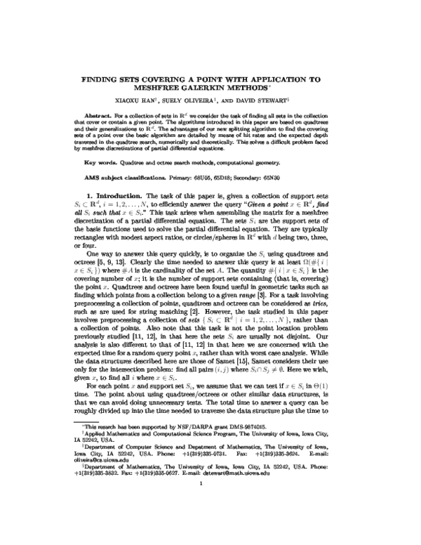S3 S2 Example of distribution of support sets Si perform the tests to identify the support sets is to have a hit (i.e., x ∈ Si ) x. Sin e the best we an do, ∈ Si , we are interested in the ontaining whenever we test for  x hit rate, whi h is the ratio of hits to the total number of tests, averaged over all the integration points. In parti ular, we don't want this to go to zero; and if the hit rate an be bounded away from zero, then the number of tests is, at worst, proportional to the average overing number of the sets { Si | i = 1, 2, . . . , N }. We will show that O((log N )/d) for both the average time to traverse the quadtree is no worse than algorithms that we will present, so that the traversal time is a more easily ontrolled ost. Worst- ase deterministi rate is zero if x is not bounds for the hit rate an be arbitrarily bad: the hit overed by any support set and at least one test is done for x. there are no restri tions on the shape of the support sets then quadtrees/o trees be made to perform badly, for example, by making the In pra ti e, the support sets Si Si 's If an urves or thin ribbons. are dis s, balls, re tangles, or re tangular solids, or similar shapes, with modest aspe t ratios (the ratio between the longest and smallest dimension). x Si 's. Our bounds on the hit rate are proven under the assumption that randomly and uniformly over a set S whi h ontains the union of the is hosen 1.1. Appli ation. Various new methods for solving partial dierential equations have been introdu ed whi h do not require regions in order to onstru tion of grids or triangulations of ompute approximate solutions. These are known as meshfree Partition of Unity Finite Element Methods (PUFEM), Reprodu ing Kernel Parti le Methods (RKPM), Element Free Galerkin (EFG) methods and Moving Least Squares (MLS) methods. methods; there are a number of types of meshfree methods su h as An overview of meshfree methods in general an be found in [4℄. All of these methods onstru t basis fun tions Ψi , i = 1, 2, . . . , N over the domain d of interest Ω ⊂ R from whi h a Galerkin dis retization is developed. Thus, for example, for solving the partial dierential equation −∇2 u(x) + u(x) = f (x), x ∈ Ω, u(x) = 0, x ∈ ∂Ω, where ∂Ω is the boundary of Ω, we approximate u ≈ uh Then we where uh (x) = onstru t a linear system of equations for the unknown PN h i=1 ui Ψi (x). h oe ients ui : 3 Fig. 1.2. PN j=1 Quadtree and o tree examples Kij uhj = fi for i = 1, 2, . . . , N where Kij = Z Ω
1 ∇Ψi (x)T ∇Ψj (x) + Ψi (x)Ψj (x) dV (x). 2 For most meshfree methods, there are either no analyti al formulas available for Ψi (x), or they are too omplex to ompute these integrals dire tly. Therefore numeri al approximations of the form Kij ≈ P X 1 k=1 2
∇Ψi (xk )T ∇Ψj (xk ) + Ψi (xk )Ψj (xk ) ωk are used to onstru t the linear system. In our notation, P is the number of integration points. Let Si = supp Ψi = { z | Ψi (z) 6= 0 }, the support of Ψi . Note that Ψi and all of its derivatives are zero outside its support Si . The integration points xk are s attered essentially uniformly throughout the region Ω. Rather than rst looping over i and j where Si ∩ Sj 6= ∅, and then nding all k su h that xk ∈ Si ∩ Sj , we an ompute the matrix K more e iently by looping rst over k, and then nding all i where xk ∈ Si by using quadtree/o tree type data stru tures. Note that the former strategy leads to both an interse tion nding problem and a range sear hing problem. While nding all i and j where Si ∩ Sj 6= ∅ an be solved using quadtree stru tures (see for example, Samet [15, pp. 199-225℄), the osts are at least as high as for the task dis ussed here. The problem of nding all xk where xk ∈ Si ∩ Sj is a range sear hing problem whi h requires onstru tion of a range-sear hing tree on the integration points. Apart from the fa t that the number of integration points is usually mu h larger than the number of support sets in pra ti e, these stru tures are omplex and the sear hing time omplexity is O(logd−1 P + #{ k | xk ∈ Si ∩ Sj }) in d dimensions where P is the number of integration points. By ontrast, the latter strategy an be a omplished with methods whi h have an expe ted time omplexity of just O(log N + E(#{ i | xk ∈ Si })) in any xed number of dimensions. 1.2. Quadtrees and O trees. Quadtrees and o trees are members of hierar hial de omposition data stru tures based on the prin iple of re ursive de omposition of spa e.They are widely used in image ompression [14, 13℄, GIS (Geographi Information Systems) [16, 6℄, omputer vision [7℄, and omputer graphi s [8, 17℄. Quadtrees an be used to represent a two-dimensional spa e. Similarly, o trees an be used to 4 deal with the three-dimensional ase. A quadtree is a tree data stru ture based on a re tangle with four hildren and an o tree is a tree data stru ture based on a ube with eight hildren. However, both of them an be used in the generation of meshes for nite element analysis. Due to dierent appli ations, there are variants on this stru ture, su h as region-based quadtrees, and point quadtrees. A quadtree an be des ribed in this way using Java, for example: lass QtreeNode{ private Obje t data; private QtreeNode hildren[2℄[2℄; private QtreeNode parent; private int depth; private int oords[2℄; ... } An o tree tree an be des ribed in a similar way using Java lass O treeNode{ private Obje t data; private O treeNode parent; private O treeNode hildren[2℄[2℄[2℄; private int depth; private int oords[3℄; ... } We use the following notation and terminology to des ribe various aspe ts of quadtrees, o trees and their d-dimensional analogues. • A support set Si is simply a bounded subset of Rd ; the quadtree or o tree onstru tion algorithm is , given a olle tion {Si | i = 1, 2, . . . , N } of these sets, to build a orresponding quadtree or o tree representation of these support sets Si . • A re tangle is a set of the form [a1 , b1 ] × [a2 , b2 ] × · · · × [ad , bd ] in Rd ; a −k re tangle in a quadtree or o tree has the spe ial property that ai = γi 2 , bi = (γi + 1)2−k for all i with k independent of i, and γi an integer. A subre tangle of a re tangle R in a quadtree or o tree is a re tangle in the quadtree or o tree ontained in the re tangle R. • We use quadtree to refer to quadtrees and their generalizations to 2d -trees in Rd . The term thus in ludes o trees in three dimensions and binary trees in one dimension. • The width of a set A is the diameter of the set in the innity norm; that is, width(A) = sup{ kx − yk∞ | x, y ∈ A } = supx,y∈A maxi |xi − yi |. • The top re tangle is the re tangle at the root of the quadtree or o tree. It is usually onsidered to be the re tangle [0, 1] × [0, 1] × · · · × [0, 1]. • The expe ted value of a random variable X is denoted E(X). • The d-dimensional volume, or d-volume of a set S is denoted vold (S). Ea h re tangle in the quadtree has an asso iated linked list ontaining referen es to support sets Si ; if R is a re tangle in the quadtree whose linked list ontains a referen e to Si , we say that Si is linked to R, or that R links Si . 2. Algorithms. In this Se tion we present two quadtree sear h algorithms to nd the number of support sets overing ea h point x. In our appli ation, x is an integration point and is part of a set of integration points xk that are approximately 5 Top rectangle x R1 R4 S2 R2 R3 S1 Fig. 2.1. Example of the basi quadtree Top rectangle x R1 R4 R2 R3 S2 S1 Fig. 2.2. Example of the expanded quadtree uniformly distributed in a domain Ω. The rst algorithm for building quadtree stru tures is the alled the basi algorithm, and the se ond is alled the splitting algorithm. These data stru tures onstru ted are dis ussed in Samet [15℄, where the former is alled the MX-CIF quadtree and the latter the expanded MX-CIF quadtree. In this paper these will be referred to as the basi and expanded quadtrees, respe tively. However, neither data stru ture was onsidered in Samet [15℄ in the ontext of identifying sets ontaining a given query point. The splitting algorithm has advantages over the basi algorithm in nding the number of support sets overing the integration point x. The total expe ted query time for randomly sele ted points x an be bounded in terms of the hit rate and the expe ted depth traversed in the quadtree. We will provide detailed theoreti al analysis and numeri al simulation in terms of these quantities later. We illustrate the basi and expanded quadtrees in Figures 2.1 and 2.2. In both the basi algorithm and the splitting algorithm, ea h re tangle in the quadtree has a orresponding linked list. In the basi approa h we try to link ea h Si to a re tangle R in the quadtree if it is ontained in R and there is no subre tangle of R in whi h Si is ompletely ontained. Note that Si is not ne essarily linked to a leaf node of the quadtree, even at the time of linking. Also note that there an be more than one support set linked to a single re tangle R, reating a linked list. In the interests of e ien y, we usually want these linked lists to be short. When using this 6 Check if width(Si )<width(R)/2 j R4 No R R j+1 4,2 j-1 yes: split Si ; do not link Si to R j+1 R4,3 Yes for each subrect R’ of R: if R’ contains Si then R R’ Si j+1 j+1 R3,1 R 3,4 j R3 Fig. 2.3. algorithm, in the worst time where ε = mini The basi link Si to R Example for des ribing the splitting algorithm ase, the onstru tion of the quadtree takes O(N log(1/ε)) diam Si . algorithm onstru ts a quadtree whi h is the MX-CIF quadtree dis- ussed by Samet [15, pp. 200213℄ and the data stru ture dis ussed by Abel and Smith [1℄. Unlike Samet, however, we are interested here in nding sets Si ontaining query points, rather than interse tion dete tion. Pseudo- ode for building the basi quadtree (basi algorithm) void basi (S ,top,N ) /* Constru ting a quadtree for support sets Si . */ for i = 1, 2, . . . , N R ← top repeat for ea h subre tangle R′ of R if Si ⊆ R′ R ← R′ & break for loop end if end for until (no subre tangle of R ontains Si ) link Si to the re tangle R end for For example, in gure 2.1, the subre tangle linked to R2 ; sin e S1 is not S2 is not linked to the top re tangle R but it is linked to ontained in any of the sub-re tangles of R, it is R. In our splitting algorithm (our se ond method), if a support set of a re tangle R, but is not a subset of any sub-re tangle of R Si is a subset in the quadtree and < 12 width(R), then we don't link Si to R; rather we split Si : for ′ ′ subre tangle R of R, if Si ∩ R 6= ∅ and re ursively all the splitting algorithm ′ Si ∩ R . We give the pseudo- ode for the splitting algorithm below. if diam(Si ) ea h with 7 Note that the splitting algorithm builds a re ursive extension of the MX-CIF tree of Samet whi h is the expanded MX-CIF tree of Samet [15, pp. 213215℄. Pseudo- ode for building the expanded quadtree (splitting algorithm) pro edure splitting(Si,R) /* Add support set Si to quadtree using R as the root of the quadtree */ loop if R′ is a subre tangle of R where Si ⊂ R′ R ← R′ else if diam(Si ) < 21 width (R) for ea h subre tangle R′ of R where R′ ∩ Si 6= ∅ (allo ate R′ if ne essary) all splitting(Si ∩ R′ ,R′ ) else link Si to R and exit loop end loop The splitting algorithm is illustrated by Figure 2.3. The subs ripts in this gure refer to the subre tangle number, being 1 (northwest), 2 (southwest), 3 (southeast), or 4 j+p (northeast). In this gure Rk,l,... denotes the re tangle at level j + p where k, l, . . . j−1 denotes the path from R to this re tangle within the quadtree. To onstru t the omplete quadtree, we apply splitting to all support sets, i.e. for i = 1, 2, . . . , N all splitting(Si,top) Note that in the expanded quadtree, ea h Si an be linked to more than one re tangle in the quadtree. In fa t, ea h Si an be linked to at most 2d re tangles. As given, the time and spa e requirements for the splitting algorithm are O(2d N h) where h is the depth (or height) of the expanded quadtree. Sin e splitting an produ e very small sets in the omputation of R′ ∩ Si , the worst- ase spa e and time requirements are unbounded. However, if path ompression [2℄ is used so that re tangles with only one allo ated subre tangle and no Si linked to it, are removed from the quadtree, the worst- ase spa e requirements redu e to O(2d N ). Furthermore, the depth of the path ompressed quadtree is bounded above by cmax + ⌈log2 N ⌉, where cmax = maxx #{ i | x ∈ Si } is the maximum overing number. In appli ations, the maximum overing number is bounded, or grows polylogarithmi ally in N . The path- ompressed quadtree an be built in rementally using a number of different te hniques. A path- ompressed version of the basi quadtree an start by nding the depth and o-ordinates of the smallest en losing quadtree re tangle. For ea h Si we nd a bounding box [a1 , b1 ] × · · · × [ad , bd ] ⊆ [0, 1]d , and expand ea h oordinate ai and bi in binary. The number of leading bits of ai and bi that mat h is the depth of the smallest en losing quadtree re tangle, and the mat hing bits are the (integer) oordinates of that re tangle. Using the Java data stru tures above, the urrent path- ompressed quadtree an be traversed downwards until a re tangle is found at the orre t depth, or the orre t pla e to insert a new su h re tangle an be found. On e this is found, standard te hniques an insert a suitable re tangle in O(1) time. A similar approa h an be used to nd the ≤ 2d re tangles whi h are linked to a support set for the splitting algorithm by rst nding mat hing bits. This makes the time to onstru t the quadtree for the splitting algorithm with path ompression O(2d N (cmax + log N + d log log(1/ε)) where ε = mini diam(Si ) assum- 8 ing O(1) time bit operations (and, or, invert, and shift) on integers. Alternatives to pointer-based data stru tures in lude balan ed trees and hash-tables using the tuple (depth, oord1 ,. . ., oordd) as the key, where oordi is the ith o-ordinate of the re tangle. Alternatively, if in the splitting algorithm the set R′ ∩ Si is expanded to have diameter no less than 0 < η ≤ 1/2 times the diameter of Si , the maximum depth of the expanded quadtree is no more than log2 (1/ε) + log2 (1/η). Choosing a parti ular value (e.g., η = 1/4) gives an upper bound on the depth of the expanded quadtree generated by the modied splitting algorithm with the same asymptoti behavior. Furthermore, the performan e bounds for the sear h given below remain unaltered for the modied splitting algorithm. On e the quadtree is onstru ted, we need to use it to nd the support sets overing a given point x. Below is our pseudo- ode for doing this with a quadtree onstru ted using either the basi or splitting algorithms. list fun tion sear h(x,top) /* Given x, find all Si that over x: x ∈ Si */ R ← top while R 6= null for ea h Si linked to R if x ∈ Si then add Si to list of overing support sets in rement overing number R ←allo ated subre tangle of R ontaining x, if any R ← null if there is no su h subre tangle end while In Figure 2.1, we show the behavior of the basi algorithm. We need to make a test to determine if x is in S2 or not be ause S2 is linked to the top re tangle, though x is far from S2 . In Figure 2.2, the advantages of the splitting algorithm are exemplied. We will test if a given x ∈ S2 only if it is in the two smallest re tangles shown ontaining S2 . 2.1. The advantage of the expanded quadtree over the basi quadtree. Just as we dis ussed above, in the basi quadtree there are many unne essary tests to obtain the sets overing ea h integration point. Here, we give the plot of the number of wasted tests (unne essary tests) per integration point in two algorithms in Figure 2.4. Here, we randomly generate 2000 support sets ( ir les) with radius = 0.2 and use 10000 uniformly distributed integration points. We observe that the number of wasted tests in the basi algorithm is 1520 times the number in the expanded quadtree. Figure 2.5 gives plots of the lengths of the linked lists in the basi and expanded quadtrees. We an see, for the hosen 200 support sets, that the linked lists are generally mu h shorter for the expanded quadtree, so that fewer tests are needed for ea h re tangle. Furthermore, the few re tangles with long linked lists in the basi quadtree are the top re tangles, and the re tangles near the top. All support sets linked to the top re tangle are tested for any integration point, making this data stru ture mu h less e ient. 2.2. The hit rate. The hit rate is the ratio between the average number of sets overing integration point x and the average number of tests for nding all overing sets for all integration points x, where x is a point randomly hosen from a uniform distribution of points over the top re tangle. 9 wasted test plot for the splitting algorithm 12 10 8 6 4 2 0 0 2000 4000 6000 8000 10000 12000 10000 12000 wasted test plot for the basic algorithm 200 150 100 50 0 0 2000 Fig. 2.4. 4000 6000 8000 The number of wasted tests in the basi and expanded quadtrees length of linked lists in the basic algorithm 3 # rectangles+1 10 2 10 1 10 0 10 0 20 40 60 80 100 120 # linked particles 140 160 180 200 160 180 200 length of linked lists in the splitting algorithm 4 10 3 # rectangles+1 10 2 10 1 10 0 10 0 20 Fig. 2.5. 40 60 80 100 120 # linked particles 140 The length of linked lists in the basi and expanded quadtrees 10 Basic algorithm: max. depth rectangle support set links to 2 10 1 10 0 10 0 200 400 600 800 1000 1200 support set 1400 1600 1800 2000 1800 2000 Splitting algorithm: max. depth rectangle support set links to 2 10 1 10 0 10 0 200 400 Fig. 2.6. 600 800 1000 1200 support set 1400 1600 Depth of re tangle linked to ea h support set We give a more pre ise denition of the hit rate: hit rate = E(covering#) E(#tests) Here covering# is the number of sets overing the randomly hosen point x, while #tests is the number of tests needed in the algorithms to determine the list of sets overing x. That is, hit rate is the ratio between the mathemati al expe tation of the overing (support sets) numbers of the integration points and the expe tation of the number of tests to get the overings for the randomly hosen and uniformly distributed integration points. 3. Analysis of the expe ted sear h time. We randomly hoose integration points x and go down through the quadtree to nd the sets Si whi h ontains x in our integration region. The total sear h time will depend on how many tests we will do for the integration points we use, and how deeply we traverse the tree stru ture. So our expe ted sear h time is: E(sear h time) = O(E(depth) + E(#tests)), where depth is the depth traversed in the quadtree when sear hing for sets overing a given point x, and #tests is the number of tests x ∈ Si that are performed during the sear h. Sin e E(#tests) = (hit rate) × E(covering#), provided the hit rate is bounded away from zero, we get O(E(depth) + E(covering#)) expe ted sear h time per query point. We will show that, for both the splitting and basi algorithms, the expe ted depth is bounded above by (log N )/d. i.e. E(depth) = O((log N )/d). For the basi 11 quadtree, the hit rate an go to zero. In fa t, for the basi quadtree the hit rate is O(N −1/2 ) in two dimensions in pra ti e. The expanded quadtree, however, has a hit rate that is bounded away from zero independently of N , although it an de rease exponentially as the dimension d in reases. In the following se tions we will analyze both the hit rate and the expe ted depth traversed in the quadtree. 3.1. Analysis of the hit rate. We assume bounds on the aspe t ratio, whi h is the ratio of the longest to the shortest side. First, we give the lower and upper bounds of E(covering#), then we get the inequality of ree ting relationship between E(covering#) and E(#tests). We ombine these to bound the hit rate. 3.1.1. The hit rate for the basi algorithm. First, we note that the hit rate an be arbitrarily bad for the basi quadtree. In two dimensions, if every support set Si was hosen to interse t either the horizontal or verti al lines bise ting the top re tangle, then every support set would be linked to the top re tangle of the quadtree. That would mean that all the support sets would have to be tested for all integration points x ∈ top. This would give a hit rate of E(covering#)/N , whi h an be arbitrarily lose to zero, and goes to zero if the average overing number is bounded as N → ∞. Even for uniform or random distributions of the sets Si , if diam(Si ) are all near ε > 0, the number of sets linked to the top re tangle is Θ(N ε); if ε = Ω(N −1/d ) as we would expe t if the Si 's overed top, then the number of sets linked to the top re tangle would be Ω(N 1−(1/d) ). While this is an improvement over the naive approa h of dire tly√testing a point x against all sets Si , it is far from optimal. This onrms the the O( N ) query time found in [1℄ for planar queries. 3.1.2. Using the number of links to express E(#test) for the expanded We work in d dimensions (d = 2 for quadtrees, d = 3 for o trees). Let bj be the number of re tangles whi h have at least Nj = #links at level j . Also, let N one support set linked at level j . Note that Nbj ≤ Nj , and every support set has at most 2d links to it. So, for all support sets N for the integration point x , we have quadtree. ∞ X j=0 Nj ≤ 2d N. Every re tangle at level j has d-volume 2−jd times the volume of the top re tangle and ea h link from a re tangle requires a test for any point ontained in that re tangle. Suppose that the re tangles at level j whi h are linked to a support set are Rj,1 , Rj,2 , . . . , Rj,Nb . Sin e there are Nj links at level j , then the expe ted number j of links to sear h from level j is: E(tests at level j) = bj N X P r(x ∈ Rj,k ) × (#support sets linked to Rj,k ) bj N X 2−jd (#support sets linked to Rj,k ) = 2−jd Nj . k=1 = k=1 E(#tests) is the sum of the expe ted number of links in all levels: E(#tests) = P∞So,−jd 2 Nj . j=0 12 E(covering#) for the expanded quadtree. Adding total Si , i = 1, 2, ..., N in d dimensions, we get the value of E(covering#) = E(#{ i | x ∈ Si }). Let a be the maximum aspe t ratio (the ratio of 3.1.3. Bounds on volumes of all support sets the largest side to the shortest side for re tangles) vold (top) = 1. of the support sets. Assume that Then, E(covering#) = N X vold i=1 = We suppose that, at level tree is less than 2d : j , Si 1 ad−1 (Si ) ≥ N X i=1 width 1 ad−1 width (Si )d (Si )d i=1 has nij ∞ X nij ≤ 2d j=0 N X links. Then the total links of Si in the whole i. for all j for all supports of our n . Remember that for the expanded quadtree a i ij support set Si is not linked at level j if the width of Si is no more than half the width of a re tangle at level j . That is, On the other hand, the total number of links in level integration points are: Nj = nij = 0 P (Si ) ≤ 2−j−1 width(top). if width Sin e in the expanded quadtree, the volume of add all volumes in ea h linked re tangle for vold Assuming vold (top) = 1, (Si ) ≤ Si is split into disjoint parts, if we we have the following bound: nij 2−jd vold (top). j=0 we have vold An upper bound for ∞ X Si , (Si ) ≤ E(covering#) E(covering#) ≤ = ∞ X nij 2−jd . j=0 is easily obtained: ∞ N X X nij 2−jd = i=1 j=0 ∞ X N ∞ X X nij )2−jd ( j=0 i=1 Nj 2−jd . j=0 ji∗ = min{ j | Si is linked to a re tangle R at level j }. For at least one re tangle R on level ji∗ , the aspe t ratio of Si ∩ R is no more than 2a. Then vold (Si ) ≥ vold (R ∩ Si ) ≥ P∞ ∗ (2a)1−d width(R∩Si )d ≥ (2a)1−d 2−d width(Si )d ≥ 2a(4a)−d2−(ji +1)d . Sin e j=0 nij ≤ P ∞ 2d and nij = 0 for j < ji∗ , vold (Si ) ≥ j=0 2a(4a)−d 2−(j+1)d × 2−d nij . However, what we really need is a lower bound. For ea h set Si let 13 Then, vold (Si ) So, we ≥ 2a(16a)−d an get a lower bound of E(covering#) = N X ∞ X j=0 E(covering#) vold (Si ) i=1 = 2a(16a)−d nij 2−jd as follows: ≥ 2a(16a)−d ∞ X ∞ X N X nij 2−jd j=0 i=1 Nj 2−jd = 2a(16a)−d E(#tests) j=0 d. Thus the hit rate for the expanded quadtree is bounded away from zero for xed 3.1.4. The lower bound of the average hit rate for the expanded quadtree. By the denition of the hit rate, we have lower bound for average hit rate: hit rate From here, we E(covering#) ≥ 2a(16a)−d E(#tests) = an see it is impossible to get zero hit rate in our quadtree sear h. That is to say, if ea h set Si is a square in two dimensions, for ea h set Si overing x, there will be an average of at most 128 tests using the splitting algorithm. However, this bound is not sharp: the hit rate is usually mu h larger, as an be seen in Figure 3.1 and in Table 3.1. 3.2. The simulation results on hit rate. From the point of view of the rate, we hit an also demonstrate that the advantage of the expanded over the basi quadtree. For 10000 randomly hosen and uniformly distributed integration points and 2000 support sets with radius 0.2, we get the following results. The average hit rate in the expanded quadtree is almost 30 times larger than that of in the basi expanded quadtree: 0.1694; basi of the wasted tests ase: quadtree: 0.0057. This result agrees with the result ounted in the two algorithms. Note that in this simulation, many of the support sets overlap, whi h an ause di ulties for other data stru tures. Figure 3.1 shows the hit rate plots for the basi and expanded quadtrees. Computational results were also obtained for a tual meshfree methods. In parti ular, for a two-dimensional elasto-plasti problem omputations were done using a number of dierent levels of renement. The parti ular meshfree method used was the RKPM (Reprodu ing Kernel Parti le Method) [10℄. tensor produ ts of B-splines (that is, are ubi The basis fun tions were Ψi (x) = Bi,1 (x1 )Bi,2 (x2 ) where Bi,1 and Bi,2 splines), so that the support sets were axis-aligned re tangles. The aspe t ratios of the support sets were all similar, and not extreme. However, ea h support set was relatively large, resulting in a great deal of overlap; the average overing number is around 15. Table 3.1 shows the main results. Note that #R is the number of re tangles allo ated for the quadtree, integration (i.e., query) points, and h N is the number of sets, P is the number of is the depth (or height) of the quadtree. The naive algorithm tests ea h point against ea h support set. This example does not show the full power of the data stru tures sin e the problems are relatively small and two-dimensional. However, the dieren e between the basi trees is learly evident. The average and expanded quad- overing numbers for the problems are shown 14 hit rate plot−−−splitting algorithm 1 hit rate 0.8 0.6 0.4 0.2 0 0 2000 4000 6000 sample point 8000 10000 12000 10000 12000 hit rate plot−−−basic algorithm 0.06 hit rate 0.04 0.02 0 0 2000 4000 6000 sample point Fig. 3.1. Hit rate plot in the basi Data stru ture Problem N P oarse 71 557 medium 152 1286 ne 349 3139 ne2 605 5582 ne3 985 8262 #R 4 5 12 20 20 Basi hit rate 0.2372 0.1443 0.0775 0.0516 0.0396 8000 and expanded quadtrees h 2 2 3 3 3 Expanded #R hit rate h 16 0.3904 5 42 0.3033 7 106 0.2781 7 223 0.2442 10 240 0.1937 10 Naive hit rate 0.1998 0.1058 0.0419 0.0246 0.0155 Table 3.1 Table showing quadtree statisti s for meshfree problems. in Table 3.2. As expe ted, the basi quadtree's hit rate is roughly proportional to N −1/2 , and the naive algorithm's hit rate is roughly proportional to N −1 , while the expanded quadtree's hit rate is relatively stable. There is learly additional overhead in setting up the quadtree using the splitting algorithm, but the number of re tangles allo ated is mu h less than the number of support sets, and the depth of the resulting quadtree grows only slowly, probably logarithmi ally, in N . Note that the implementation of the splitting algorithm did not use any modi ations to avoid deep quadtrees. Even so, path ompression would a hieve little here sin e the number of re tangles not linked by support sets for the splitting algorithm were, for the various problems: oarse 2; medium 6; ne 9; ne2 16. Thus for the largest problem (ne2), path ompression ould save no more than 16 of the 223 allo ated re tangles. Thus it appears that for our appli ation, path ompression will save little in spa e or time. 15 Problem Avg. overing # oarse 14.18 medium 16.09 ne 14.61 ne2 14.90 ne3 15.22 Table 3.2 Table showing average overing numbers. E(depth). As in the previous se tion, we let Nj denote the number of links at level j ; Nbj denotes the number of re tangles linked to at least one support set in level j ; and Nej denotes the number of allo ated re tangles in the quadtree at level j . Clearly, Nbj ≤ Nj . Sin e every allo ated re tangle must have P P a subre tangle that is linked to a support set, Nej ≤ ∞ Nbk ≤ ∞ Nk . On the 3.3. The upper bounds of k=j k=j dj other hand, Nej ≤ 2dj sin e there are at most P∞2 re tangles in a quadtree at level j . Note from the previous se tion that j=0 Nj ≤ N for the basi quadtree, but P∞ d j=0 Nj ≤ 2 N in the expanded quadtree. 3.4. Analysis of E(depth). Re all that depth is the depth of the quadtree traversed while sear hing for the sets overing a given point x, hosen at random. The basis of these al ulations are bounds on the probability of depth having a parti ular value. A detailed dis ussion on related issues an be found in [2℄. E(depth) = = = ∞ X j=0 ∞ X j=0 ∞ X j=1 j Pr(depth = j) j [Pr(depth ≥ j) − Pr(depth ≥ j + 1)] Pr(depth ≥ j). The problem now is to bound Pr(depth ≥ j). This is the probability that x lies in an allo ated re tangle at a depth j . A simple bound is Pr(depth ≥ j) = 2−dj Nej ≤ 2−dj min(2dj , 2d N ) = min(1, 2−d(j−1) N ). This leads to bounds of the form E(depth) = O(log N ): E(depth) = ≤ Suppose that 2d(j Thus ∗ −1) ∞ X j=1 ∞ X Pr(depth ≥ j) min(1, 2−d(j−1) N ). j=1 < N ≤ 2dj . Then for j ≥ j ∗ , 2−d(j−1) N ≤ 2−d(j−j ∗ ∗ E(depth) ≤ j X 1+ j=1 = j∗ + ∞ X 2−d(j−j j=j ∗ +1 ∞ X −dl 2 l=0 = j∗ + ∗ −1) 1 ≤ j ∗ + 2. 1 − 2−d ∗ −1) ≤ 1. 16 Note that j ∗ = ⌈(log2 N )/d⌉, and so  log2 N E(depth) ≤ d  +2=O  log2 N d  . 4. Con lusions. The expe ted total sear h time using the expanded quadtree for a random point x ∈ top is O(E(depth)) + O(E(#tests)). Sin e the number of tests needed is the overing number divided by the hit rate (whi h is bounded below by 2a(16a)−d) we get an expe ted sear h time whi h is O((log N )/d + (16a)d E(#{ i | x ∈ Si })). For xed d, this is O(log N + E(#{i | x ∈ Si })). This means that for appli ations where the overing number grows at least as fast as log N , we have an asymptoti ally optimal method. Otherwise, the expe ted time for the sear h grows like O(log N ) whi h, while not asymptoti ally optimal, still gives good performan e. By omparison, the expe ted total sear h time for the basi quadtree is Θ(N ) for a worst ase olle tion of sets {Si }, and Θ(N 1−1/d ) for olle tions of sets whi h o ur in pra ti al problems. A knowledgments. We would like to thank Prof. J.S. Chen and his students Hui-Ping Wang and Cheng-Tang Wu for providing the meshfree method odes on whi h the omputational results in Tables 3.1 and 3.2 are based. We would also like to thank the referees whose omments have helped to improve this paper. REFERENCES [1℄ D. J. Abel and J. L. Smith. A data stru ture and algorithm based on a linear key for a re tangle retrieval problem. , 24(1):113, 1983. [2℄ Arne Andersson and Stefan Nilsson. Faster sear hing in tries and quadtreesan analysis of level ompression. In Jan van Leeuwen, editor, , pages 8293. Springer, Berlin, 1994. Le ture Notes in Computer S ien e #855. [3℄ Arne Andersson and Kurt Swanson. On the di ulty of range sear hing. , 8(3):115122, 1997. [4℄ T. Belyts hko, Y. Krongauz, D. Organ, M. Fleming, and P. Krysl. Meshless methods: An overview and re ent developments. , 139:347, 1996. [5℄ Mark de Berg, Mar van Kreveld, Mark Overmars, and Otfried S hwarzkopf. . Springer-Verlag, Berlin, 1997. Algorithms and appli ations. [6℄ P. Gao and T. R. Smith. Spa e e ient hierar hi al stru tures: Relatively addressed ompa t quadtrees for GISs. , 7:173177, 1989. [7℄ I. Gargantini and H. H. Atkinson. Linear quadtrees: a blo king te hnique for ontour lling. , 17:285293, 1984. [8℄ Donald Hearn and M. Pauline Baker. . Prenti eHall., 1994. [9℄ Mi hael J. Laszlo. . Prenti e Hall, In ., Upper Saddle River, NJ, 1996. [10℄ S. Li and W. K. Liu. Reprodu ing kernel hierar hi al partition of unity: Part I: Formulation and theory. , 45(3):251288, 1999. [11℄ M. H. Overmars. Point lo ation in fat subdivisions. , 44:261265, 1992. [12℄ F. P. Preparata and R. Tamassia. Fully dynami point lo ation in a monotone subdivision. , 18(4):811830, 1989. [13℄ Hanan Samet. The quadtree and related hierar hi al data stru tures. , 16(2):187260, 1984. [14℄ Hanan Samet. . Addison-Wesley, 1990. [15℄ Hanan Samet. . Series in Computer S ien e. Addisonwesley, Reading, MA, 1990. [16℄ Cliord A. Shaer, Hanan Samet, and Randal C. Nelson. A geographi information system based on quadtrees. , 4,2:103 131, 1990. Computer Vision, Graphi s and Image Pro essing AlgorithmsESA '94 (Utre ht) Comput. Geom. Computer Methods in Applied Me hani s and EngiComputational neering geometry Pattern Re ognition Image and Vision Computing Computer Graphi s, 2nd Edition, C Version Computational geometry and omputer graphi s in C++ Internat. J. Numer. Methods Engineering Infomation Pro . Letters SIAM J. Computing Appli ations of Spatial Data Stru tures The Design and Analysis of Spatial Data Stru tures Comput. Surveys International Journal of Geographi Information Systems 17 [17℄ K. Yamagu hi, T. L. Kunii, K. Fujimura, and H. Toriya. O tree-related data stru tures and algorithms. IEEE Computer Graphi s and Appli ations, 4(1):5359, 1984.