The Design of the Bow 1
B.W. Kooi
Abstract
The invention of the bow and arrow probably ranks for social impact with the invention of the art of kindling a fire and the invention of the wheel. It must have been
in prehistoric times that the first missile was launched with a bow, we do not know
where and when. The event may well have occurred in different parts of the world
at about the same time or at widely differing times.
Numerous kinds of bows are known, they may have long limbs or short limbs,
upper and lower limbs may be equal or unequal in length whilst cross-sections of the
limbs may take various shapes. Wood or steel may be used, singly as in ‘self’ bows,
or mixed when different layers are glued together. There are ‘composite’ bows with
layers of several kinds of organic material, wood, sinew and horn, and, in modern
forms, layers of wood and synthetic plastics reinforced with glassfibre or carbon. The
shape of the bow when relaxed, may be straight or recurved, where the curvature of
the parts of the limbs of the unstrung bow is opposite to the way they are flexed to
fit the string.
In previous papers we have dealt with the mechanics of the bow and arrow. The
main subject of this paper is the design and construction of bows. Nondimensionalization of the problem leads to the introduction of the maximum elastic energy
storage capacity per unit of mass as a material constant for strength. At the same
time a coefficient is derived which measures the effectiveness of the form of the crosssection of a bending beam.
The assumption that the limbs of a bow are fully loaded implies a relationship
between a number of design parameters. It reduces the dimension of the design
parameter space. When the strength of materials is taken into account constraints
are imposed on a number of design parameters. This defines feasible regions.
Sensitivity analysis gives the influence of a number of important parameters on
quality coefficients, one of these is proportional to the amount of available energy and
other are the efficiency and the velocity of the arrow at the onset of its flight. These
quality coefficients measure the performance of a bow for specific purposes such as
hunting, flight shooting and target shooting.
We compare the performance of bows used in the past with that of modern competition bows. It appears that the superb features of man-made materials contribute
most to the better performance of the modern bow and not its geometric shape.
1
Proceedings Koninklijke Nederlandse Akademie van Wetenschappen 97(3): 1–27 (1994)
�1
Introduction
A number of disciplines is involved in the design of the bow. One, technology, a discipline
in which processability, strength, fracture mechanics, fatigue, maintenance and resistance
to atmospheric action, are subjects of interest. Bowyers (manufacturers of archery equipment) have to cope with such questions as the influence of temperature changes on the
performance of the bow and of course with the availability of materials. In the Middle Ages,
when longbows were made in huge quantities in England, the fine-grained yew, Taxus baccata, was imported from Spain and it was compulsory to import consignment of Spanish
bowstaves with each shipment of Spanish wine.
Two, the working of the bow as a mechanical device can be described by mathematical
formulations of physical laws, e.g. Newton’s law or the principle of Hamilton. The action of
the bow before departure of the arrow from the string is called interior ballistics. Exterior
ballistics deals with the flight of the arrow through air.
Three, the success of the archer depends largely upon his or her skill. For, when
mechanical systems are used to launch arrows, the point of impact is approximately the
same for each shot. Small deviations may occur due to differences in the mass of the arrow
or wind-velocity/direction. Thus an archer will try to perfect a technique that produces
a repeatable shot, and he or she must gain experience in coping with changing weather
conditions.
In the past bowyers relied heavily upon experience for the design of the bow. The
performance of the bow was improved by the ‘try and cut’ method. The bowmaker was
a craftsman and he made his bows very much as his father had done before him, any
improvements being strictly empirical, he did not write books about it — apprentices
learned their craft by word of mouth and practical demonstration. In the 1930’s bows
and arrows became objects of study by scientists and engineers, for example by Hickman,
Klopsteg and Nagler, see [5–7].
In previous papers, [8–12] we dealt with the mechanics of the different types of bow:
non-recurve, static-recurve and working-recurve bows. The main subject of this paper is
the design of the bow. We will formulate the problem in the terminology of the optimization
theory for mechanical structures. It is thus clear that the strength of materials used in
making a bow, is dealt with. We consider only bows of traditional design, consisting of a
bent stick with a grip in the middle. We do not deal with newer developments in which
mechanical devices such as pulley’s and springs are used to improve the design, see [1,13,14].
The problem is formulated and different types of bow are defined in Section 2. All
design parameters are charted accurately and quality coefficients are defined. Besides real
number parameters there are three functions of the length coordinate along the limbs, i.e.
bending stiffness, mass distribution and geometric shape of the unstrung bow, giving rise
to an intricate design process. The importance of the application of dimensional analysis
will be dealt with.
The mechanics of the bow is dealt with in Section 3. However, we are engaged only in
aspects related to the design of the bow and this makes this paper self-contained. For a
complete discussion of the mathematical formulation of the problem and the derivation of
1
�the numerical techniques the reader is referred to former papers, [8–12]. The mechanical
performance of bows belonging to different types, is reported. Each ‘standard’ bow is
supposed to represent a bow used in different parts of the world in the past or the present
at archery contests such as the Olympic Games. As to the mechanical performance, these
bows are much the same and the differences cannot explain the large variation in shooting
performance observed in reality.
The subject of Section 4 is the design and construction of the bow where the technological properties of the materials used to make bows are taken into account and the
manner in which these materials are applied in bows is considered. Dimension analysis
yields two useful quantities. One is the energy storage capacity per unit of mass of the
material. The allowable amount for a particular bow–arrow combination depends on the
failure mode (fracture, de-lamination, buckling, fatigue, creep) of the limbs. Two, a dimensionless shape-factor of the cross-section of the limbs. This measures the usage of the
material in bending.
It is shown that the type of the bow and the properties of the material used are strongly
related. Assumptions with respect to a uniform loading along the limbs yield relationships
between the design parameters. This reduces the dimension of the design parameter space.
Constraints imposed by technological requirements, such as strength, set bounds in the
design parameter space. The differences in the performances of the different types of bow
can be explained by these feasible regions.
In Section 5 we perform a sensitivity analysis for a number of design parameters in
the feasible regions. One of the most important parameters is the mass of the arrow. In
practice there is a constraint either on the mass itself, or on the ratio of the arrow mass
and mass of the bow. This leads to the introduction of a nominal draw and nominal weight
of a bow. They depend on the type of bow and on the materials used. When the weight
and draw of a bow equal these nominal values the velocity of the lightest usable arrow is
maximal. The sensitivities appear to be different depending on whether the actual weight
is larger or smaller than the nominal weight of the type of bow.
In the literature the importance of a large amount of available energy in the fully drawn
bow is always stressed. We also analyse sensitivities with respect to this quantity. It is not
a design parameter, however, and we discuss how to interpret these sensitivities. Many
authors when describing and discussing the famous Turkish flight bow, assign its good
performance to its ears. These ears provide leverage and allow more energy to be stored in
the bow. Stiff ears, however, are also heavy and therefore diminish efficiency so that the
energy of the arrow differs little from that of other types of bow. In addition to this, we
show in this paper that part of the good static performance is counteracted by the large
amount of elastic energy in the braced bow. This implies heavier limbs to store this extra
useless energy and this also reduces the dynamic performance of the bow.
In Section 6 the performance of a number of ancient and a modern bow are compared.
It turns out that the application of better materials and a better usage of these materials
contributes most to the improvement of the bow.
2
�a)
Figure 1: Three situations of the non-recurve bow: a) unbraced, b) braced, c) fully drawn.
a)
Figure 2: Three situations of the static-recurve bow: a) unbraced, b) braced, c) fully drawn.
2
Classifications of bows
In this paper we deal only with bows that are symmetric with respect to the line of aim.
The bow is placed in a Cartesian coordinate system (x, y), the line of symmetry coinciding
with the x-axis and the origin O coinciding with the midpoint of the bow.
We assume the limbs to be inextensible and the Euler-Bernoulli beam theory to be valid.
The total length of the bow, measured along it, is denoted as 2L. The bending stiffness
W (s) and mass per unit of length V (s) are both functions of the length coordinate s
measured along the bow from O. In Figure 1(a) the unbraced situation (without string) is
shown. The geometry of the bow is described by the local angle θ0 (s) between the elastic
line and the y-axis, the subscript 0 indicates the unstrung situation. L0 is half the length
of the grip and 2mg denotes its mass.
3
�a)
Figure 3: Three situations of the working-recurve bow: a) unbraced, b) braced, c) partly drawn.
In Figure 1(b) the bow is braced by applying a string. The length of the unloaded string
is denoted as 2l0 , its mass by 2ms . We assume that the material of the string obeys Hooke’s
law, longitudinal stiffness is denoted as U s . Note that either the length of the string or the
brace height, denoted as |OH|, fixes the shape of the bow in the braced situation.
Classification of the bow is based on geometric shape and the elastic properties of the
limbs. The bow of which the upper half is depicted in Figure 1, is called a non-recurve
bow. These bows have contact with the string only at their tips (s = L) with coordinates
(xt , y t ). In the unstrung situation these coordinates are design parameters of the bow and
are denoted as (xt0 , y t0 ). There may be concentrated masses mt with moment of inertia J t
at each of the tips, representing for example horns used to fasten the string. The simple
straight-end bow and the English longbow, and the composite Angular bow are non-recurve
bows. Simple bows made out of one piece of wood, straight and tapering towards the ends,
have been used by primitives in Africa, South America and Melanesia. Ancient composite
bows, e.g. the Angular bow used in Egypt and Assyria, consisted of layers of several kinds
of organic materials, wood, sinew and horn.
In the static-recurve bow, see Figure 2, the outermost parts of the limbs are stiff.
These parts are called ears. The mass of each ear and its moment of inertia with respect
to the centre of gravity (xcg , y cg ) are denoted as me and J e , respectively. The flexible part
L0 ≤ s ≤ L2 is called the working part of the limb. Some Tartar, Chinese, Persian, Indian
and Turkish composite bows are static-recurve bows. In the braced situation the string
rests upon string-bridges, see Figure 2(b). These string-bridges are fitted to prevent the
string from slipping past the limbs. The position of the bridge on the upper limb is referred
to as (xb , yb ). When such a bow is drawn, at some moment the string leaves the bridges
and has contact with the limbs only at the tips.
With a working-recurve bow the parts near the tips are elastic and bend during the
final part of the draw, see Figure 3. When drawing such a bow the length of contact
between string and limb decreases gradually until the point where the string leaves the
4
�limb, denoted as s = sw , coincides with the tip s = L. It remains there during the
final part of the draw. We assume that there is no friction between bow and string for
sw ≤ s ≤ L. Today almost all bows seen at target archery events, are working-recurve
bows. The core of these modern composite bows is made of wood, for instance Maple, with
layers of synthetic plastics reinforced with glassfibre or carbon on both sides. In Figure
3(c) the bow is pulled by force F (b) into a partly drawn position where the middle of the
string has the x-coordinate b. To each bow belongs a value b = b1 = |OD| for which it
is called fully drawn. Values of variables in this situation are indicated by a subscript 1.
The force F (|OD|) is called the weight of the bow and the distance |OD| is its draw . The
arrow, represented by a point mass 2ma , is propelled towards its target by releasing the
drawn string at time t = 0 and holding the grip of the bow at its place. During acceleration
at some specific point in time t = tb the string again touches the belly side of the limb of
a static-recurve or working-recurve bow.
In practice, the connection between the end or nock of the arrow and the string is not
loose as is assumed usually. It is stated that the strength of this connection, called the
nock tension, should be such that the arrow will just hang on the bow string without falling
off. We assume that this nock-tension is zero, then the arrow leaves the string when the
acceleration of the midpoint of the string becomes negative. This moment is denoted as
tl and its velocity at that moment is called muzzle velocity or initial velocity of the arrow
which is denoted as cl . The arrow in its flight is slowed down by the drag or resistance of
the air. The exterior ballistics is beyond the scope of this paper. We do, however, deal
with the vibratory motion of the bow limbs after arrow exit.
A shorthand notation for a bow and arrow combination is introduced as follows
B(L, L0 , W (s), V (s), θ0 (s), ma , mt , J t , me , J e , mg , xcg0 , y cg0 , xb0 , y b0 , xt0 , y t0 , L2 ,
(1)
U s , ms , |OH| or l0 ; |OD|, F (|OD|), mb ),
where mb is the mass of one limb excluding the mass of the grip and including the mass of
the ears.
The quantities |OD|, F (|OD|) and mb are taken as the elements of a dimensional base in
a dimensional analysis. The first factor is limited by the length of the bowman’s arms, from
the left hand fully extended to the right hand, drawn back beside the right shoulder. The
second one is linked up with the bowman’s muscle. In addition it depends on the ability
of the fingers of the right hand to control the string, to hold it during aiming and release
it at the right moment. The third factor is a limitation of the strength of the materials
used. Quantities with dimension are labelled by means of a bar ‘ ’ and quantities without
the bar are the associated dimensionless quantities.
Note that the two latter parameters the weight of the bow F (|OD|) and the mass of
the limbs mb have been added to the list artificially. This implies that both functions W (s)
and V (s) are constrained. Both functions, bending stiffness W (s) and mass distribution
V (s) are considered to be the product of the functions W (s)/W (L0 ) and V (s)/V (L0 ) of
the length coordinate s into R and parameters W (L0 ) and V (L0 ) with dimensions. These
resulting functions together with the function θ0 (s) make the bow a distributed parameter
5
�structure. Thus the values of the functions W (s) and V (s) for s = L0 are already fixed by
two constraints. The first constraint relating to weight, is an implicit relationship between
a number of parameters, of which W (s) is one, and the weight F (|OD|) = 1 of the bow.
The second constraint is
Z L2
V (s)ds + me .
(2)
mb = 1 =
L0
2.1
Quality coefficients
The purpose for which the bow is used has to be considered in the definition of a costfunction that should be optimized to obtain the ‘best’ bow. It appears, however, to be
very difficult to define such a cost-function uniquely. Therefore we introduce a number
of quality coefficients which can be used to judge the performance of a bow and arrow
combination.
In the past the bow was used for hunting and warfare requiring a good arrow penetration
capacity. High arrow kinetic energy at the moment of impact and perhaps also a large
linear momentum are indispensable. Initial velocity must be high enough to ensure a
flat trajectory of the arrow. Nowadays archery has become a sport, for target shooting
accuracy is most important. This means that the action of the bow should not exaggerate
small differences in the parameters caused by slight differences in the handling of the bow
by the archer during the shooting.
In flight shooting, it is tried to shoot an arrow as far as possible. When the drag during
the flight of the arrow is neglected, for maximum range its initial velocity must be as large
as possible and the angle of departure must be 45◦ with the horizontal.
We will now define three dimensionless quality coefficients. First, the static quality
coefficient q is given by
A
q=
|OD| F (|OD|)
and A =
Z
b=|OD|
F (b)db ,
(3)
b=|OH|
where A is the energy stored in the elastic parts of the bow, the working parts of the
limb and the string, by deforming the bow from the braced position into the fully drawn
position. Hence, A measures the total amount of energy available for the acceleration of
the arrow. The static quality coefficient is large when the shape of the Static Force Draw
curve F (b) is a concave function. It is small when the drawing force rises very sharply in
the last part of the draw. In this case, while aiming, the archer has to hold a relatively
large force to obtain a certain amount of available energy. Furthermore the available energy
depends more sensitively on the actual draw length. Notice that q can be larger than 1
but is generally about 0.5.
Second, the shooting efficiency η defined by
η=
ma c2l
,
A
6
(4)
�where cl is again the initial velocity, is a dynamic quality coefficient. Using the principle
of stationary potential energy we can show that under general conditions we have η ≤ 1.
When the braced situation is the only stable equilibrium the potential energy possesses an
unique minimum. Therefore the potential energy in the bow at arrow exit is larger than
or equal to this minimum and as a result the difference with the potential energy in the
fully drawn position is generally smaller for the shape at arrow exit than it is in the braced
situation. Thus even when the velocity of the limb is zero we generally have η ≤ 1. When
there are more than one local minima for the potential energy in the braced situation we
could have η ≥ 1. In [12] we dealt with this phenomenon. A bow with a very flexible part
of the limbs near the tip had three braced shapes, two stable and an unstable equilibrium of
the bow without an external force. Drawing from the largest of the two local minima, the
shape of the bow at arrow exit could be close to the shape of the braced bow belonging to
the smallest minimum of the potential energy, the global minimum. Before the next shot,
the archer has to put the bow in the other stable braced situation again before drawing
the bow. This extra amount of energy is not taken into account in our definition of the
efficiency, but it is available for the acceleration of the arrow.
In [12] we showed that theoretically a shooting efficiency of 100% can be obtained if
the limbs of the bow are taken to be rigid with all the elasticity to be concentrated in
two elastic hinges and an inextensible string without mass. This simple model shows the
principle of the bow very clearly, because of geometrical constraints the velocity of the
relatively heavy limbs at arrow exit is small, while the very light string is connected to the
fast moving arrow. This implies that the kinetic energy of the moving parts of the bow
at arrow exit is relative small and therefore almost all available energy is transferred, as
kinetic energy, to the high speed light arrow.
The initial velocity of the arrow then follows from Equations (3) and (4), being
s
q
qη |OD| F (|OD|)
= ν dbv ,
cl =
(5)
ma
mb
where we introduced a factor dbv and the dimensionless initial velocity referred to as ν
according to
r
qη
|OD| F (|OD|)
and ν =
,
(6)
dbv =
mb
ma
respectively. This dimensionless initial velocity ν is taken as the third quality coefficient.
This is determined by the other two coefficients, q Equation (3), η Equation (4) and the
dimensionless mass of the arrow ma .
The efficiency η depends highly on the mass of the string. This influence can be assessed
using a simplified model in which we assume that the string remains straight between the
points of attachment at the tip of the bow and the nock of the arrow. The resulting
distribution of the kinetic energy along the string indicates that 1/3 of the mass of the
string should be added to the arrow after which the string can be taken without mass.
7
�Then,
max(η) ≈
ma
,
ma + 31 ms
(7)
gives an approximation of the maximum attainable efficiency. The reason is that for the
unrealistic simple model with the two rigid limbs described above, but now adding a string
with mass moving in the manner assumed above, the efficiency would be equal to the
right-hand side of Equation (7).
Klopsteg improved Equation (7) by stating that a certain part of the deformation energy
A is converted into kinetic energy of the arrow, the string and the bow limbs. He suggested
the formula
A = (ma + K h ) c2l ,
(8)
where 2K h is the virtual mass. This quantity can be estimated from measured velocities
for different arrow masses or can be calculated using a mathematical model. However, it
accounts as we see later on not only for the moving limbs, but also for the elastic energy in
the limbs and the string, exceeding the value of the elastic energy in the braced situation
referred to as AH . Klopsteg states:“That the virtual mass is in fact a constant, has been
determined in many measurements with a large number of bow”. Experiments described
in [18] with a modern working-recurve bow confirmed Klopsteg’s rule very well. In the
next sections we will therefore use the following expression for efficiency
η=
ma
,
ma + Kh
(9)
where Kh is the dimensionless half virtual mass. The quantity Kh is, just as is the efficiency
η, a function of dimensionless parameters, however, it does not depend on ma . This rule
is not based on a physical law, we found in [9] that it was not supported by the results
obtained with our mathematical model for a straight-end bow.
Observe that by definition the quality coefficients q, η and ν mentioned above are
dimensionless. This means that the quality coefficients measure the quality of the bow and
arrow combination under comparable conditions; the same weight, draw and mass of the
limbs.
In an input–output philosophy all parameters in Equation (1) are input variables which
determine the mechanical action of the bow and arrow combination. In this notation B
stands for the set of output variables in which one is interested, for instance the quality
coefficients.
3
The mechanics of the bow and arrow
In our mathematical model the action of a bow and arrow is fixed by one point in a
24 dimensional parameter space, of which 3 parameters are functions of s into R, see
8
�Equation (1). In what follows we study a number of standard bows each representing
different sorts of bow. These different sorts used in the past and at present, form clusters
around these standard bows in the parameter space. We consider the three types of bow:
two non-recurve bows, namely the Straight-end bow (for instance the Longbow) and the
Angular bow; two Asian static-recurve bows and two working-recurve bows, one with an
extreme recurve and a modern working-recurve bow. The static deformation shapes of all
these bows are shown in [10].
For the functions W, V, θ : [L0 , L] → R we assume a simple form:
L−s
, L0 ≤ s ≤ L − ǫ(L − L0 ) ,
L − L0
W(s) = ǫW(L0 ) , L − ǫ(L − L0 ) ≤ s ≤ L ,
W(s) = W(L0 )
(10)
where W is W or V . If not stated otherwise the shape of the unstrung bow is given by
θ0 (s) = θ0 (L0 ) + κ0
L−s
, L0 ≤ s ≤ L .
L − L0
(11)
The two parameters W (L0 ) and V (L0 ) are already fixed by the requirement that |OD|,
F (|OD|) and mb are equal to 1. Under this description, these functions are fixed by only
three parameters ǫ, θ0 (L0 ), a measure for the reflex of the grip, and κ0 , a measure for the
recurve of the unstrung limbs in a circular arc.
We start with a straight-end bow described by Klopsteg in [5]. This bow is referred to
as the KL-bow and it represents among others the simple bows used by primitives all over
the world and the famous English longbow.
The values for all the parameters are given in Table 1. W, V and θ are given in Equation (10) with ǫ = 1/3 and Equation (11) with θ0 (L0 ) = 0 and κ0 = 0.
The AN-bow represents the Angular bow found in Egypt and Assyria. For this bow
the bending stiffness and mass distribution W (s) and V (s) are given in Equation (10) with
ǫ = 1/3 and L0 = 0, while θ0 (s) is given by
¡ |OH| ¢ s
− , 0 ≤ s ≤ L − ǫL ,
L
L
¡ |OH| ¢ £ s
L − s ¢2 ¤
1¡
−
ǫ−
, L − ǫL ≤ s ≤ L .
−
θ0 (s) = arcsin
L
L 2ǫ
L
θ0 (s) = arcsin
(12)
This function gives, in the braced position, the characteristic triangular shape.
Now we consider two static-recurve bows found in China, India or Persia, called the PEbow, and one from Turkey, called the TU bow. The bending stiffness and mass distribution
of these two bows W (s), V (s) and the shape of the unstrung bow, θ0 (s) are given in
Equation (10) with ǫ = 1/3 and Equation (11) for L0 ≤ s ≤ L2 with θ0 (L0 ) = 0 and
κ0 = 0. For the TU-bow all the parameters are equal to those of the PE-bow except
κ0 = −2.0 and adapted values for xcg0 , ycg0 , xb0 , yb0 , xt0 , yt0 so that the ears equal those of
the PE-bow are placed in line with the working part of the limbs at s = L2 .
9
�Table 1: The complete set of design parameters for the standard bows studied. The
parameters used to make the parameters dimensionless are: |OD|, F (|OD|) and m b . For
all bows we have: mt = 0, Jt = 0 and mg = 0.
Bow
KL
AN
PE
ER
L
L0
W (s), ǫ in Eqn. (10)
V (s), ǫ in Eqn. (10)
θ(s)
ma
me
Je
xcg0
ycg0
xb0
yb0
xt0
yt0
L2
Us
ms
|OH|
1.286
0.1429
1/3
1/3
Eqn. (11)
0.0769
0
0
—
—
—
—
0
1.286
—
131
0.0209
0.214
0.7857
0
1/3
1/3
Eqn. (12)
0.0769
0
0
—
—
—
—
−0.1551
0.7427
—
131
0.0209
0.214
1.0
0.1429
1/3
1/3
Eqn. (11)
0.0769
0.4
0.0025
−0.0464
0.7589
0
0.7857
−0.1856
0.8929
0.5714
131
0.0209
0.25
1.151
0.2075
1/32
1/32
Eqn. (11)
0.0769
0
0
—
—
—
—
−0.4153
0.5824
—
131
0.0209
0.214
10
�One example of a working-recurve bow possesses an excessive recurve and is called the
ER-bow. It resembles a bow described and shot by Hickman, see [5]. The bending stiffness
distribution is given by Equation (10) with ǫ = 1/32, while θ0 (s) given by Equation (11)
with θ0 (L0 ) = 0.8404 and κ0 = −3.3537.
The energy values for different parts of these bows in various situations are shown in
Table 2. These values indicate that for bows with strongly recurved limbs, the amount of
energy in the braced situation (referred to as AH ) is high (for the KL-bow AH = 0.1226
while for the TU-bow we calculated AH = 1.0867 and for the ER-bow even AH = 1.4260).
At arrow exit the stored potential energy is, for all bows, higher than in the braced situation
(for instance for the AN-bow 0.1765 and 0.1576, respectively). This shows that K h accounts
also for the excess of the elastic energy and that it is not solely an added mass accounting
for the kinetic energy of the limb and string. The amount of energy in fully drawn situation,
stored in the elastic parts of the bow is referred to as AD . It is equal to Ab + As , where Ab
is the amount of elastic energy in the limbs and As in the string, of the fully drawn bow.
For example for the ER-bow we have AD = 1.415 + 0.012 = 1.426.
The three calculated quality coefficients for these types of bow are shown in Table 3.
The static quality coefficient q is given by: q = AD − AH with AD and AH given in Table
2. For example for the PE-bow we have q = 0.5932 − 0.1625 = 0.432. The quantity Ab , the
elastic energy in the fully drawn limbs (already given in Table 2) is also given because this
quantity will play an important role in the design of the bow dealt with in Section 4. The
efficiency of the strongly recurved ER-bow is rather bad η = 0.810/0.3374 = 0.417 and
this undoubtedly counteracts the very good static quality coefficient q = .810. Obviously,
the tips of the limbs are decelerated less efficiently.
The values of the quality coefficients for a modern working-recurve bow are also given
in Table 3. This WR-bow is described in [8]. The dimensionless mass of the arrow and
string of this bow were respectively ma = 0.0629 and ms = 0.0222. With these masses the
calculated quality coefficients are given in [11]: the efficiency is η = 0.729 and the initial
velocity ν = 2.23. The values for the efficiency η and initial velocity ν shown in Table 3
were adjusted for the values ma = 0.0769 and ms = 0.0209 using Klopsteg’s rule (9) taking
(7) into account by the assumption that the term 1/3 ms is part of the virtual mass Kh .
The results indicate that the initial velocity ν is about the same for all types! So, within
certain limits, the dimensionless parameters which determine the mechanical performance
of the bow for flight shooting, appear to be less important than is often claimed.
The acceleration force E acting on the arrow plus the added mass of the string 1/3 ms
is defined by
1
E = −2 (ma + ms )ċ , t ≥ 0 .
3
(13)
where c = ḃ is the dimensionless velocity of the arrow. Another important quantity is the
recoil force P , being the force the bow exerts on the bowhand of the archer.
These forces E, P and the force in the string K as a function of time t are shown in
Figure 4. After arrow exit at time t = tl in Figure 4 the acceleration force E is the force
acting on the added mass representing the string. As can be seen E oscillates around zero
11
�Table 2: Energy distribution for a number of bows in three situations: braced, fully drawn
and arrow exit
energy
limbs
pot.
kin.
string
pot.
kin.
total bow
pot.
kin.
arrow
kin.
KL-bow
braced
fully drawn
arrow exit
0.0950
0.5155
0.0663
0
0
0.0491
0.0276
0.0137
0.0681
0
0
0.0344
0.1226
0.5292
0.1344
0
0
0.0835
0
0
0.3112
AN-bow
braced
fully drawn
arrow exit
0.1461
0.5493
0.1380
0
0
0.0573
0.0115
0.0033
0.0385
0
0
0.0359
0.1576
0.5526
0.1765
0
0
0.0932
0
0
0.2961
PE-bow
braced
fully drawn
arrow exit
0.1515
0.5879
0.1271
0
0
0.0980
0.0100
0.0053
0.0506
0
0
0.0279
0.1625
0.5932
0.1777
0
0
0.1271
0
0
0.2884
TU-bow
braced
fully drawn
arrow exit
0.5755
1.081
0.5324
0
0
0.1346
0.0204
0.0053
0.0844
0
0
0.0312
0.5959
1.0867
0.6168
0
0
0.1658
0
0
0.3040
ER-bow
braced
fully drawn
arrow exit
0.419
1.415
0.564
0
0
0.3511
0.197
0.012
0.087
0
0
0.0756
0.6160
1.4260
0.6510
0
0
0.4266
0
0
0.3374
12
�Table 3: Dimensionless quality coefficients for the standard bows. The dimensionless half
mass of the arrow and string of the modern competition WR-bow are ma = 0.0629 and
ms = 0.0222. The efficiency η and initial velocity ν of the WR-bow have been adjusted for
the reported masses using Klopsteg’s rule. The stiffness of its string is about twice those
of the other bows.
Bow
q
η
ν
ma
ms
W (L0 )
V (L0 )
Ab
KL-bow
AN-bow
PE-bow
TU-bow
ER-bow
.407
.395
.432
.491
.810
.765
.716
.668
.619
.417
2.01
1.92
1.94
1.99
2.08
.0769
.0769
.0769
.0769
.0769
.0209
.0209
.0209
.0209
.0209
1.4090
0.2385
0.2304
0.1259
0.3015
1.575
2.300
1.867
1.867
2.120
0.5155
0.5493
0.5879
1.0817
1.4150
WR-bow
.434
.770
2.09
.0769
.0209
2.5800
1.950
0.6930
for t ≥ tl . The maximum force in the string occurs after arrow exit and it is larger than
in the fully drawn situation. This explains why flight shooters let their string break after
each shot. A weaker and therefore lighter string yields a higher efficiency η and initial
velocity ν.
The results of Tables 2 and 3 show that the modern working-recurve bow WR is a good
compromise between the non-recurve bow and the static-recurve bow. The recurve yields
a good static quality coefficient q and the light tips of the limbs give a high efficiency η.
Figure 5 shows the bending moment M as a function of the length coordinate s − L0 for
successive times before (Figure 5(a)) and after (Figure 5(b)) arrow exit for the WR-bow.
The broken line represents the distribution along the limb in the static braced situation.
The static bending moment M(s) is the force in the string K times the distance h(s) as
shown in Figure 3(c). This static bending moment is zero when the string lies against the
limb near the tip. The distribution along the elastic part of the limb M1 (s − L0 ) in the
fully drawn bow is also shown in Figure 5(a) and (b).
It follows from Figure 5 that M(s, t) is smaller than M1 (s) except for the part of the
limb near the grip after the arrow has left the bow. The differences are small, so we
assume that the maximum loading bending moment occurs in the fully drawn situation
and it equals M1 (s). In reality there is always internal and external damping which forces
the bow and string to return to the braced situation. This reduces the actual bending
moments for large t.
13
�Figure 4: Acceleration force E, string force K and recoil force P for the WR-bow. Moment of
arrow exit is t = tl .
a)
b)
Figure 5: Distribution of the bending moment along the limb of the WR-bow (a) before arrow
exit t ≤ tl and (b) after arrow exit t ≥ tl . The broken line represents the distribution along the
limb in the static braced situation. The bending moment M 1 (s − L0 ) in the fully drawn bow is
also shown in both figures.
14
�4
The design of the bow
The limbs of the bow can be considered to be a beam of variable cross-section D(s) made
out of one material with density ρ and Young’s modulus E. Assumption of the EulerBernoulli hypothesis yields the following relationship between the bending moment M (s, t)
and the normal stress σ(s, t, r), with r the distance from the neutral axis which passes
through the centroid of the cross-section
M (s, t) r
σ(s, t, r) = R
,
2
r
dD
D(s)
(14)
where we neglected the influence of the normal and shear forces in the limbs.
In the previous section we showed that it is acceptable to assume that the maximum
bending moment for each s as a function of time t occurs in the fully drawn situation.
Then we have, with Ab again the elastic energy in the limbs of the bow in fully drawn
situation,
2
Ab
=
mb
RL R
L0
2
1 σ 1 (s,r)
D(s) 2
E
dD ds
RL
,
(15)
ρC(s) ds
L0
R
where C(s) = D(s) dD is the area of the cross-section. Thus ρC(s) = V (s) is the mass
distribution along the limb. The stress σ 1 is the resulting normal stress due to the bending
moment in the fully drawn bow, indicated by the subscript 1.
Two additional useful quality coefficients are defined by
δ bv
σ2
= w
2 ρE
,
aD =
RL R
L0
1 2
σ (s, r) dD ds
D(s) 2 1
1 2
σ
2 w
RL
,
(16)
C(s) ds
L0
where σ w is the working stress of the material, equal to the yield point or the ultimate
strength divided by a factor of safety and the quantity δ bv is the amount of energy which
can be stored per unit of mass in the material. Then
Ab
= 2aD δ bv .
mb
(17)
In Table 4 an estimation of δ bv for some materials used in making bows, is given.
The maximum value for the dimensionless coefficient aD equals 1 in the homogeneous
stress-state σ 21 (s, r) = σ 2w for all s and r. However, aD is generally smaller than 1 for two
reasons.
First, the stress in the fibres near the neutral axis is smaller than the working stress
and this reduces the coefficient aD . Suppose the stress in the outermost fibres equals the
15
�Table 4: Mechanical properties and the energy per unit of mass δ bv for some materials used
in making bows, see also [3].
material
σw
N/m2 107
E
N/m2 1010
ρ
kg/m3
δ bv
Nm/kg
steel
sinew
horn
yew
maple
glassfibre
70.0
7.0
9.0
12.0
10.8
78.5
21.0
.09
.22
1.0
1.2
3.9
7800
1100
1200
600
700
1830
130
2500
1500
1100
700
4300
working stress for all s, in this case the limb is called uniformly stressed , then we have for
each cross-section due to bending
σ 1 (s, r) = σ w
r
,
e(s)
(18)
where e is the largest of the two distances between the outermost fibres and the neutral
axis. For a uniformly stressed bow, aD is maximum for the given D(s). If the material
has the same strength in tension and compression, it will be logical to choose shapes of
cross-section in which the centroid is at the middle of the thickness of the limb, equal to
2e(s). Then
R L I(s)
ds
L e(s)2
,
(19)
aD = R L0
C(s)
ds
L0
where I(s) is the moment of inertia of the cross-section with respect to the neutral axis. The
quantity EI(s) = W (s), already introduced in Section 2, is the distribution of the bending
stiffness along the limb. The quantity 2I/e is called the section modulus. The magnitude of
the moment of inertia and the section modulus are tabulated for various profile sections in
commercial use in various handbooks. For the assessment of the shape of the cross-sections
we stay with the dimensionless coefficient aD which follows in a straightforward manner
from our statement of the problem.
We will now consider the function αD (s) defined by
αD (s) =
I(s)
, L0 ≤ s ≤ L ,
C(s) e(s)2
16
(20)
�Table 5: Values of αD for various shapes of cross-section of limbs
shape of the cross-section D
αD
rectangular
elliptical
D-shaped
elliptical ring; 1/4(1+k 2 ), k = 0.9
0.333
0.250
0.255
0.453
rectangular
elliptical
D-shaped
belly side
elliptical ring
compression
neutral axis
height
width
di
back side
tension
do
di = k • d o
Figure 6: Different shapes of the cross-section of the bow.
for various shapes of cross-section of limbs. For a bow with geometrically similar crosssections at different values of s, αD (s) is uniform and aD = αD (s). In that case the ratio of
similarity with respect to the shape for s = L0 is a function of s. Generally, this function
is smaller than 1 for L0 < s ≤ L.
In Table 5 values of αD are given for the rectangular, elliptical, D-shaped and elliptical ring cross-sections shown in Figure 6. The English longbow possessed a D-shape
cross-section, the belly side approximately formed by a semi-circle, the other side being a
rectangle. When the radius of the semi-circle equals the half of the thickness of the limb,
αD equals 0.255, hence smaller than 0.333 for a rectangular shape and larger than 0.25 for a
elliptical shape. This magnitude for the D-shape may be conservative. As the shape is not
symmetric with respect to the neutral axis, the tensile stress at the back remains smaller
than the working stress if the same kind of wood is used throughout the limb. The back of
such a yew bow, however, was usually made of white sapwood which has a lower Young’s
17
�modulus than the red heartwood used for the belly side, see [16]. Hence, the neutral axis
is moved toward the belly side to compensate for the shift due to the semi-circular shape
of the belly. Furthermore experiments showed the sapwood of yew to be stronger than the
heartwood and this indicates that this combination of the material used and shape of the
cross-section can yield a good design.
Steel bows, for instance the Seefab bow invented in the 1930’s, are designed on the
principle of a flattened tube. We assume that the inner major axis di equals k times the
outer major axis do of the concentric ellipses. For k = 0.9 the value of αD may become
0.4525, so larger than the other values mentioned. This is to be expected because relatively
more material is placed near the outermost fibres.
There is still another technique to increase the value of aD . In ancient Asiatic bows,
horn and sinew, together with wood, were used on the belly and back, respectively. Horn
is a superb material for compressive strength and sinew laid in glue has a high tensile
strength, see Table 4. The Young’s modulus of both materials is rather small, but the
permissible strain is very high. This shows that the difference of the curvature of the axis
of the limb between fully drawn and unstrung situation has to be large, or the thickness
of the limb has to be large to load these materials to the full extent. In the latter case the
space between the two materials near the outermost fibres is filled in with light wood, which
has to withstand the shearing stresses and keep the horn and sinew sufficiently apart. In
modern bows horn and sinew are replaced by synthetic plastics reinforced with glassfibre
or carbon. So, in composite bows not only are better materials used, but they are also
used in a more profitable manner. For composite bows we define equivalent quantities for
the Young’s modulus and density so that it has the same mechanical action with respect
to bending as the simple bow made out of one kind of material. If these magnitudes are
substituted in the product aD δ bv this product can be substantially larger than for simple
wooden bows.
Second, the tensile and compressive stresses in the fully drawn bow in the outermost
fibres of the limb, in the back and the belly respectively, may be less than the working
stress. For materials with reduced strength in compression and greater strength in tension,
as is the case in most woods, the advisable cross-section for the limb will not be symmetrical
with respect to the neutral axis, but will be such that the distance from the neutral axis
to the most remote fibres in tension and compression are in the same ratio as the working
stresses, σ w , of the material in tension and compression. Note that even for a symmetrical
cross-section the neutral axis does not coincide with the line of symmetry when the Young’s
moduli for tension and compression are not equal. For wood the neutral axis lies closer
to the outermost fibres in tension than to the outermost fibres in compression because the
modulus in tension is generally larger than in compression. With the design of the limbs
one has to assure stability of the limb, without tendency to twist or distort laterally when
the bow is drawn. In practice this is accomplished by the requirement that the width of
a limb may not become smaller than its thickness, in this case material near to the tips is
not used to the full extent.
18
�Table 6: An estimation of maximum thickness of the limbs for a number of types of bow,
|OD| = 0.7112 m.
Material Bow
type
W (L0 )
M1 (L0 ) σ w
E
2
7
N/m 10 N/m2 1010
e(L0 )
m
thickness(L0 )
m
yew
sinew
horn
sinew
horn
KL
PE
PE
TU
TU
1.41
0.23
0.23
0.12
0.12
1.02
0.64
0.64
0.64
0.64
11
7
9
7
9
1
0.09
0.22
0.09
0.22
0.0112
0.020
0.010
0.0133
0.0055
0.022
0.030
sinew
yew
KL
TU
1.41
0.12
1.02
0.64
7
11
0.09
1
0.0765
0.0016
4.1
0.019
0.153
0.0032
The construction of the bow
In practice the manufacturer wants to make a bow with a specified draw |OD| and weight
F (|OD|) by the use of available materials with a given Young’s modulus E, density ρ and
working stress σ w . The equation which makes W (s) dimensionless reads
EI(s) = W (s) |OD|2 F (|OD|) .
(21)
Equations (14), (18) and (21) show that the thickness of the limb associated with the
distance e between the outermost fibres and the neutral axis is determined by
e(s) =
I(s)
W (s) σ w
σw =
|OD| .
M1 (s) E
M 1 (s)
(22)
These calculations can be done after selecting the static dimensionless parameters L, L0 ,
θ0 (s), xcg0 , ycg0 , xb0 , yb0 , xt0 , yt0 , L2 , Us and |OH| or l0 . The solution of the governing static
equations yields M1 (s). We recall that we assume that the maximum bending moment
occurs in the fully drawn situation. In Section 3 we saw that this is allowed for realistic
situations. After the selection of the shape of a cross-section of the limbs D(s), the width
is determined by Equation (21). To ensure stability this width should not be taken smaller
than the thickness of the limb. There after the area of the cross-section C(s) can be
calculated. C(s) and the density ρ jointly determine the mass per unit length V (s) and
with the length of the limbs L the mass of the limbs mb . This completes the design of the
limbs with aD as large as possible, depending on the chosen D(s).
19
�We now have the information to calculate the dimensionless mass distribution V (s).
The equation which makes V (s) dimensionless reads for L0 ≤ s ≤ L,
V (s) = V (s)
M12 (s) aD
|OD|
=
.
mb
αD (s)W (s) Ab
(23)
The mass of the limb mb is derived from Equation (17)
mb = Ab
|OD| F (|OD|)
.
2aD δ bv
(24)
When the product aD δ bv is known, the three quantities |OD|, F (|OD|) and mb of the
dimensional base are mutually dependent. This shows that, when technology is taken into
account, it would be better to take the quantity δ bv as the third element of the dimensional
base instead of the mass of the bow. We adhere to the mass of the limb in order to be
consequent with the theory on the mechanics of the bow and arrow, derived in [8–12]. The
design and construction of the bow is complete after the remaining parameters ma , mt , Jt ,
me , Je , mg , ms are selected.
Hence, in a uniformly stressed bow with αD (s) = aD along the limbs, the mass distribution V (s) depends on other dimensionless parameters given in Equation (1), see (Equation 23). Other parameters given in Equation (1) are also mutually dependent in practice,
for example the parameters relating to the ears, me , J e , xcg0 , y cg0 , xb0 , y b0 , xt0 , y t0 , L2 are
strongly related.
The same reflections on energy storage capacity can be given for the materials of the
string. To reduce the mass of the string strong materials should be used which are able to
store large amounts of elastic energy for a given mass. Many kinds of fibre have been used
for making strings. In the past natural fibres were used, animal fibres (silk and sinew) and
vegetable fibres (hemp, linen, cotton and strips of bamboo or rattan) and Belgian strings
made of long-fibered Flemish flax have been famous. Recently, man-made fibres such as
Dacron, Kevlar and Twaron were developed. Note that, except for the loop with which it
is fastened to the bow, the material throughout the cross-section of the string is uniformly
stressed. The maximum force determines, together with the strength of the material, the
minimum mass of the string. Dynamic computer simulations, see Figure 4, show that
maximum force does not occur in the fully drawn situation. So, there is a relationship
between the string parameters, U s , ms and the strength of the material used for the string,
and the maximum force in the string. This force is not known from static calculations, so
an initial guess has to be made, which must be checked after the dynamic calculations.
In practice two string-parameters, the mass ms and the stiffness U s , are for a particular
string material fixed by the number of strands. An increase of this number, to be denoted as
ns , makes the string stiffer (generally this implies a higher initial velocity) but also heavier
(and this counteracts the advantage of a stiffer string). This is a simple example that
shows how technological considerations can reduce the dimension of the design parameter
space.
20
�We can calculate the thickness of the limbs near the grip (s = L0 ) for different types of
bow made of the different materials. The distance e between the outermost fibres and the
neutral axis calculated using Equation (22) is shown in Table 6. The results demonstrate
that the yew of the longbow combined in the long straight-end bow and sinew, horn and
wood combined in the static-recurve bow, are good combinations, while yew in the staticrecurve bow and sinew, horn and wood in the long straight-end bow are not, showing that
in practice it is not possible to interchange geometric shape and material in the construction
of a bow. We therefore consider only combinations applied generally in the next section.
We will not work out a comprehensive optimization program for the efficiency, initial
velocity or amount of kinetic energy in the arrow, in the reduced design parameter space
of Equation (1), with constraints for the draw, weight and the maximum amount of energy
storage in the material and, possibly, a minimum initial velocity and a minimum mass of
the arrow as side conditions. Instead, in the next section we perform a sensitivity analysis
within the feasible region for a restricted number of design parameters and in Section 6 we
consider a number of different types of bow used in the past and up to present times. We
assume that the bow is uniformly stressed in the fully drawn situation, so that αD (s) = aD
along the limbs. We also assume Klopsteg’s rule which makes it possible to uncouple
dynamics from statics. Solution of the dynamic behaviour with a single mass of the arrow
and string yields an estimation for the parameter Kh which depends solely on static design
parameters. Klopsteg’s rule Equation (9) then yields the performance of the bow with
other arrow and string masses.
5
Sensitivity analysis
The influence of a number of the design parameters on the performance of the bow is dealt
with in this section. We will focus on the initial velocity which needs to be as large as
possible for flight shooting.
When we neglect the elastic energy stored in the string, the equation for the initial
velocity and the kinetic energy of the arrow follow from
r
q η
q
aD δ bv and ma c2l = 2 mb
η aD δ bv ,
cl = 2
(25)
Ab ma
Ab
respectively.
Hence, the initial velocity of an arrow depends on the ratio of the static quality coefficient q and the amount of elastic energy stored in the fully drawn limbs, Ab , on the ratio
of the efficiency η and the dimensionless mass of the arrow ma and finally on the product
aD δ bv . The kinetic energy is linearly dependent on the mass of the bow, mb , whereas it is
independent of the mass of the arrow.
When the mass of the arrow itself is a design parameter instead of the dimensionless
mass of the arrow, it is advantageous to define a coefficient which resembles dbv but instead
21
�of being based on the mass of the limb mb it is based on the mass of the arrow ma
|OD| F (|OD|)
.
ma
(26)
q η dav and ma c2l = q η |OD| F (|OD|) .
(27)
dav =
Then
cl =
q
When in what follows the influence of one arbitrary parameter is analysed, all other
dimensionless parameters, the draw |OD|, weight F (|OD|) and maximum energy storage
capacity aD δ bv remain unchanged.
5.1
Influence of the mass of the arrow
Equations (25) and (27) suggest that for a large velocity the mass of the arrow ma and ma
should be as small as possible. The partial derivatives of the dimensionless initial velocity
ν and of cl with respect to ma (Equations (5) and (6)), are given by
r
√
−1/2 q
∂ν
∂cl
∂ν
2
=
=
aD δ bv ,
and
(28)
3/2
∂ma
(ma + Kh )
∂ma
∂ma Ab
respectively, where we used Klopsteg’s rule Equation (9). The first one is always negative,
so the mass of the arrow should be as small as possible. We used the fact that the virtual
mass Kh is independent on the mass of the arrow ma . Then Equation (27) and (9) for
lim ma ↓ 0 yield
r
q
max(cl ) =
dbv and lim (ma c2l ) = 0 .
(29)
ma ↓0
Kh
Klopsteg [5] called this quantity max(c
p l ) the figure of merit of a bow. In the dimensionless
formulations we have max(ν) = q/Kh . Obviously no arrow shot with this bow could
achieve higher velocity than max(cl ) of Equation (29).
Klopsteg’s rule is, however, violated for small values of ma . For small arrow masses the
acceleration force will already be negative before the bow is back in its braced situation.
Furthermore, our assumption that the maximum bending moment equals the value in
the fully drawn situation, M1 (s), is then obviously violated. Every archer knows that
it is not correct to release a fully drawn bow without an arrow. In this case efficiency
equals 0, see Equation (29), and the bow or string may break. This shows that there is a
minimum value for ma . This value will depend on the type of bow represented by the other
dimensionless parameters of Equation (1) and this relationship is complex. We assume that
this minimum, denoted as Ma , is given by Ma = min(ma ) = 0.03. This value is based on
the results of computer simulations of a large number of bow arrow combinations, see [9].
There are also limits with respect to the real mass of the arrow. One has to bridge the
distance between the middle of the string and the grip. To reduce the mass of the arrow
22
�Table 7: An estimation of the nominal weight F(D) with D = 0.7112 m, of a number
of types of bow for minimum arrow masses, that means 2ma = 2Ma = 0.01 kg and
ma = Ma = 0.03 so that 2mb = 0.33 kg.
Material
Bow
type
aD
δ bv
Nm/kg
Ab
D F(D)
Nm
F (D)
N
yew
sinew,horn,wood
sinew,horn,wood
glassfibre,maple
KL
PE
TU
WR
0.255
0.5
0.5
0.33
1100
2000
2000
3000
0.52
0.59
1.10
0.70
180
564
303
476
260
800
420
670
the Turk shot flight arrows shorter than the draw of the bow. This was made possible by
using a horn groove (‘siper’) which they wore on the thumb or strapped to the wrist of
the bow hand. Further, the arrow must be strong enough to withstand the acceleration
force. We conclude that in practice there also seems to be a minimum, for the mass of
the arrow. Suppose that this minimum, denoted as 2Ma , is 2Ma = min(2ma ) = 0.01 kg.
This minimum might be a function of the weight of the bow when buckling of the arrow
is the driving phenomena behind the constraint. So, in this case also the minimum value
depends in a complex way on the other design parameters.
Combining both minimum values, the associated mass of the bow limbs becomes 2mb =
0.33 kg. We assume that the product aD δbv is known. This value determines the maximum
stored energy Ab by the use of Equation (24). For a yew bow with a D-shaped cross-section
the value for this product equals about 0.255 1100 = 280.5 Nm/kg, see Tables 4 and 5.
Therefore the maximum allowable stored energy max(Ab ) becomes about 93 Nm. For
a straight-end KL-bow the dimensionless quantity Ab = 0.52 and therefore the product
|OD| F (|OD|) = 180 Nm. When the draw length is assumed to be |OD| = 0.7112 m the
maximum allowable weight of the bow becomes F (|OD|) = 260 N. We call this weight the
nominal weight F (D) for a draw called the nominal draw D. So,
D F(D) =
2Ma aD δbv
.
Ma Ab
(30)
The nominal weight of a bow is fixed by its type (Ab ) as well as by its construction (aD δ bv ).
The nominal draw D is chosen equal to the ‘span’ of the archer.
Table 7 shows the data for each type of bow in combination with the materials of
which they are commonly made. A value of 0.5 was chosen for aD with the composite
bow with sinew, horn and wood. This value is larger than 0.25 (the value for the elliptical
23
�cross-section) and takes into account the better usage of the material. The exact value
is difficult to obtain as to do this the thickness of each layer must be known. The values
for the quantity δ bv are combinations of those given in Table 4 for the materials used in
making the bows. Those for Ab are taken from Table 3. We will use these results in Section
6 where we compare these nominal weights with data given in the literature.
For the bowyer it is now important to know whether the desired weight is larger or
smaller than the nominal weight. We assume that the dimensionless parameters including
Ma and also 2Ma together with the energy storage parameter aD δ bv are already chosen.
We will now discuss the influence of the weight F (|OD|).
If F (|OD|) > F(D) then the bowyer must use more material and accordingly the mass
of the limbs mb becomes larger. This can be done by increasing the width of the limbs
proportionally but leaving the thickness, as given by Equation (22), unchanged, but, the
value for ma , which is now a design parameter, was already as small as possible, so the
archer has to use a heavier arrow (ma > Ma ) when he wants to shoot such a strong bow.
In this case all dimensionless design parameters remain the same and therefore he does
not gain a larger initial velocity, but the kinetic energy increases proportionally with the
weight, see Equations (26) and (27).
If F (|OD|) < F(D) the bowyer can remove some wood from the sides of the limbs.
The mass of the arrow ma , which is now a design parameter, can not be lowered, and
therefore the dimensionless mass of the arrow becomes larger (ma > Ma ). This gives a
better efficiency, but the negative effect of a smaller weight is stronger. For a given mass
of the arrow the influence of the weight stems from the term η F (|OD|) in Equation (27).
The partial derivative of this term with respect to the weight of the bow equals, using
Klopsteg’s rule Equation (9) and Equation (17),
∂η
∂(η F (|OD|))
Kh
= η + F (|OD|)
= η (1 −
).
ma + Kh
∂F (|OD|)
∂F (|OD|)
(31)
Hence, initial velocity decreases for decreasing weight smaller than the nominal value.
These considerations show that for each combination of material and type of bow there
is a nominal value for the product draw times weight which determines the maximum
obtainable initial velocity (efficiency equal to 1) and it is given by Equations (26) and (27)
s
D F (D)
.
(32)
max(cl ) = q
Ma
5.2
Influence of the strength of material
When ma is a design parameter (F (|OD|) > F(D)) the advantage of a large value of
the product aD δ bv is clear from Equation (33). When, however, ma is taken as a design
parameter (F (|OD|) < F(D)), the effect of a larger value of this product is neutralised by
a larger value of ma , better materials imply a lighter bow and therefore a larger ma . The
advantageous effect of better materials (larger δ bv ) or a better use of the materials (larger
24
�aD ) stems in this case solely from the higher efficiency η. In the limit for δ bv ↑ ∞ we have
mb ↓ 0 and ma ↑ ∞, and this implies for the efficiency η ↑ 1. In this case the drawn bow
returns quasi-statically to the braced situation.
5.3
Influence of the static quality coefficient
In the literature a high value for the static quality coefficient q is often mentioned as a
requirement of a good bow, see for instance [5–7]. Therefore it is interesting to study the
influence of this quantity.
Substituting Klopsteg’s rule, Equation (9) into Equation (25), we obtain for the velocity
r
q
1
aD δbv .
cl = 2
(33)
Ab ma + Kh
When the dimensionless arrow mass ma is taken as a design parameter (F (|OD|) >
F(D)), the first factor of the right-hand side of Equation (33) shows that the amount of
energy AH in braced situation, stored in the elastic parts of the bow, the limbs plus the
string should be as small as possible. This can be explained as follows. The amount of
energy AD stored in the elastic parts in fully drawn situation is given by AD = Ab +As . The
data given in Table 2 for the KL-bow show that AH = 0.1226, Ab = 0.5155, As = 0.0137
and AD = 0.5292. The static quality coefficient q is given by q = Ab + As − AH . This
contemplation shows that a large q implies a large Ab .
Authors often stress the advantage of large recurve yielding a large static quality coefficient q, however, when the energy storage capacity in materials is taken into account,
part of this advantage is offset by the relatively large energy contents of the braced bow.
The results given in Table 2 show that for the TU-bow AH = 0.5959 and for the ER-bow
AH = 0.6160 while for the KL-bow we have AH = 0.1226.
When the mass of the arrow ma is a design parameter (F (|OD|) < F (D)), q and ma in
Equation (33) are mutually dependent, as a large q implies heavy limbs and this in turn
yields a small ma , because it is the arrow mass divided by the mass of one limb. In the
case of a given mass of the arrow ma and therefore fixed dav , the influence of q originates
from the term q η in Equation (27). We therefore calculate the partial derivative of this
product with respect to q. The use of Klopsteg’s rule Equation (9) and Equation (17)
together with AH assumed to be constant, gives
∂η
q
∂(q η)
Kh
=η+q
= η(1 −
),
∂q
∂q
Ab ma + Kh
(34)
this quantity is always positive. So, we conclude that in this case a large static quality
coefficient q is advantageous for both the initial velocity cl and the kinetic energy ma c2l .
The coefficient q is not a design parameter but a quality coefficient and thus a function of the dimensionless parameters which determine the static performance of the bow.
Therefore we assumed in our derivation that it is possible to change the design parameters
of Equation (1) so that the virtual mass Kh of the bow remains the same. In this way
25
�Table 8: Parameters with dimension for a number of bows and an estimation of aD , using
Equation (17), and of the nominal weight F (D) with D = |OD|.
Ref. Bow
type
[5]
[4]
[2]
[16]
[15]
[18]
flatbow
longbow
steelbow
Tartar
Turkish
modern
KL
KL
KL
PE
TU
WR
F (|OD|) |OD|
N
m
2mb
kg
2L
m
δ bv
Ab
Nm/kg
aD
F(D)
N
155
465
170
460
690
126
0.325
0.794
0.709
1.47
0.35
0.29
1.829
1.874
1.689
1.88
1.14
1.703
1100
1100
130
2000
2000
3000
0.20
0.25
0.69
0.07
0.77
0.07
198
236
81
107
656
141
0.7112
0.746
0.7112
0.7366
0.7112
0.7112
0.52
0.52
0.52
0.59
1.1
0.70
the influence of the static and dynamic coefficients on the initial velocity are separated
completely. To manage this, it may be difficult to find a combination of adaptations of the
design parameters. In reality such a combination does perhaps not exist, for instance, in
the previous section we found that a larger q for a number of types of bow unfortunately
was accompanied with a smaller efficiency. This holds for the TU-bow and certainly for
the ER-bow as well.
The results obtained in this section show that the sensitivity of the velocity with respect
to energy storage capacity and the static quality coefficient is different for F (|OD|) < F (D)
and F (|OD|) > F(D). For F (|OD|) = F (D) the initial velocity is a maximum.
6
Comparison of a number of ancient and modern
bows
In this section we consider a number of ancient bows described in the literature, [2,4,5,15,16]
and one modern bow described in [18]. In Table 8 we give values for the parameters
with dimension, weight, draw and mass of one limb. Estimations of aD which have to
be compared with the values given in Table 5 were calculated using Equation (17). The
approximation of aD has to be rough for lack of detailed information.
These results indicate that the short Turkish bow is made of a combination of good
materials which are used to the full extent. The calculated value aD = 0.77 is rather high,
αD = 0.25 for an elliptic cross-section, see Table 5. Observe that the chosen value for δ bv
is just the average of those for sinew and horn, for a better evaluation the thickness of the
different layers should also be taken into account, but this detailed information is missing.
If we take aD = 0.77 instead of aD = 0.5, used to calculate the value F (D) = 420 N
26
�mentioned in Table (7), we obtain F(D) = 656 N and the weight of the short Turkish bow
is F (|OD|) = 690 N. So for this bow the weight is close to the nominal weight. The large
amount of energy stored per unit of mass in the limbs explains the good performance of
the Turkish bows in flight shooting, and not the mechanical performance of these bows;
see Table 2.
The estimations of aD for the flatbow and the longbow are very realistic. For an
rectangular cross-section αD = 0.33 and for an D-shaped cross-section αD = 0.255, see
Table 5. Note that the nominal weight for the flatbow is rather close to the weight of this
bow. Indeed, Klopsteg designed this bow based on theoretical insight obtained by Hickman
in [5]. For the steelbow, the estimation aD = 0.69 is also close the value for αD = 0.453.
For both the Tartar bow and the modern the estimated value for aD = 0.07. This
indicates that not all the materials are used to its full extent. Observe that these bows are
not used for flight shooting. For the Tartar bow the materials near the tips, namely that
for the bridges, are stressed only partly. This results in a small efficiency.
For the modern working-recurve bow there is a surplus of material near the grip. An
efficiency of 72.9% for the modern working-recurve bow is rather low. The maximum efficiency according to Equation (7) from the mass of the string determined by the parameters
given in Table 3 is about 90%. This shows that with respect to this aspect, the design of
the modern bow can be improved.
7
Conclusions
We conclude that the results indicate that the dimensionless initial velocity is about the
same for all types of bow under similar conditions. So, within certain limits, the design
parameters which determine the mechanical action of a bow-arrow combination appear to
be less important than is often claimed.
Introduction of technological constraints and realistic assumptions about the crosssection of the limbs, yield a relationship between the distribution of the mass and bending
stiffness along the limbs. This reduces the dimension of the design parameter space. It is
advantageous to define the two nominal quantities of draw and weight. These depend on
the type and construction of the bow. The sensitivity of the initial velocity with respect
to design parameters is different depending on whether the weight is larger or smaller than
the nominal weight. In the one case the dimensionless mass of the arrow and in the other
the mass itself is a design parameter. The maximum initial velocity occurs when the weight
of the bow equals the nominal weight for the type of bow considered. This maximum lies
on the boundary of the feasible region with respect to the mass of the arrow.
It appears that the material properties of yew combine very well with the straight-end
type of bow and the material properties of the composites, wood, sinew and horn combine
very well with the static-recurve bow. A combination of many technical factors made the
composite flight bow better suited for flight shooting.
After the recovery in 1982, of the Mary Rose, Henry’s VIII’s flagship which sank in the
Solent in 1545, numerical modelling gave a good insight into the mechanical performance
27
�of the famous English longbow, used for instance at Agincourt during the Hundred Years’
War between England and France, [17], and many other battles.
This shows that mathematical modelling is a helpful tool in the archery research, both
for the design of new bow equipment and also for an understanding of the historical development of the bow.
The quality coefficients of the modern bow are only slightly better than those of the
historical bows. Materials used in modern working-recurve bows can store more deformation energy per unit of mass than materials used in the past. Moreover the mechanical
properties of these materials are more durable and much less sensitive to changing weather
conditions. This contributes most to the improvement of the modern bow.
In this paper we have demonstrated the need to state the bow design problem in terms
of structural optimization theory. Mathematical formulation helps with the systematic
identification of all the design parameters. Sensitivity analysis yields the most important
design parameters. Together with simplicity assumptions, this reduces the number of
design parameters and makes the design process surveyable. This allows us to clarify the
differences in the performance of bows found all over the world by the introduction of
technological constraints.
8
Acknowledgement
The author wishes to acknowledge the discussions with Prof. dr. J.A. Sparenberg and Prof.
ir. M. Kuipers. He thanks Miranda Aldham-Breary for correcting the English.
References
[1] R. B. Arinson. The compound bow: Ugly but effective. Machine Design, pages 38–40,
nov 1977.
[2] R. P. Elmer. Target Archery. Hutchinson’s Library of sports and pastimes, London,
1952.
[3] J. E. Gordon. Structures or Why Things Don’t Fall Down. Pelican, Harmondsworth,
1978.
[4] R. Hardy. Longbow. Mary Rose Trust, Portsmouth, 1986. pp. 4-6.
[5] C. N. Hickman, F. Nagler, and P. E. Klopsteg. Archery: the technical side. National
Field Archery Association, Redlands (Ca), 1947.
[6] P. E. Klopsteg. Bows and arrows: a chapter in the evolution of archery in America.
Technical report, Smithsonian Institute, Washington, 1963.
[7] P.E. Klopsteg. Turkish archery and the composite bow. Simon Archery Foundation,
Manchester, 1987.
28
�[8] B. W. Kooi. On the mechanics of the bow and arrow. Journal of Engineering Mathematics, 15:119–145, 1981.
[9] B. W. Kooi. On the Mechanics of the Bow and Arrow. PhD thesis, Rijksuniversiteit
Groningen, 1983.
[10] B. W. Kooi. The ’cut and try’ method in the design of the bow. In H. A. Eschenauer,
C. Mattheck, and N. Olhoff, editors, Engineering Optimization in Design Processes,
volume 63 of Lecture Notes in Engineering, pages 283–292, Berlin, 1991. SpringerVerlag.
[11] B. W. Kooi. On the mechanics of the modern working-recurve bow. Computational
Mechanics, 8:291–304, 1991.
[12] B. W. Kooi and J. A. Sparenberg. On the static deformation of a bow. Journal of
Engineering Mathematics, 14:27–45, 1980.
[13] C. Mattheck. Optimization of the static behaviour of a new high energy bow and
arrow. XVI. International Finite-Element Congress, Baden-Baden, November 1987.
[14] N. Mullaney. Buckle bow .. a new twist. Archery World, pages 38,60–61, March 1978.
[15] Sir R. Payne-Gallwey. The Crossbow. Holland Press, London, 1976.
[16] S. T. Pope. Bows and Arrows. University of California Press, Berkeley (CA), 1974.
[17] G. Rees. The longbow’s deadly secrets. New Scientist, pages 24–25, June 5 1993.
[18] C. Tuijn and B. W. Kooi. The measurement of arrow velocities in the students’
laboratory. European Journal of Physics, 13:127–134, 1992.
29
�
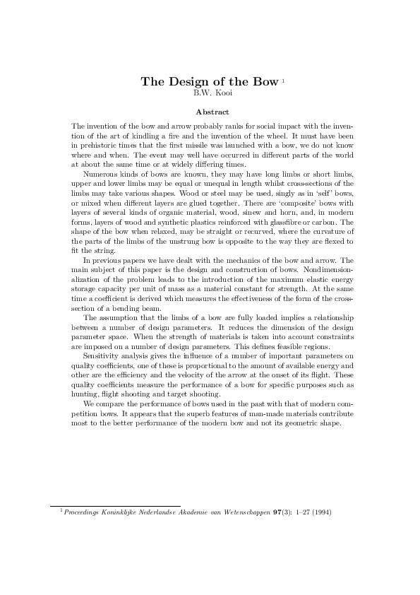
 Bob Kooi