
Copernicus Sentinel-2A Calibration and Products Validation Status

 , , ,
, , , <p>Multi-Spectral Instrument (MSI) internal configuration. <b>Left</b>: full instrument view (diffuser panel in yellow, telescope mirrors in dark blue). <b>Right</b>: optical path construction to the Short-Wave Infrared (SWIR)/visible to near-infrared (VNIR) (see <a href="#sec2dot2-remotesensing-09-00584" class="html-sec">Section 2.2</a>) splitter and focal planes.</p> "> Figure 2
<p>MSI spectral bands vs. spatial resolution with corresponding Full Width at Half Maximum (FWHM).</p> "> Figure 3
<p>Staggered Detector Configuration.</p> "> Figure 4
<p>Line of Sight angles definition.</p> "> Figure 5
<p>Representation of the pixels Line-Of-Sight (LOS) projection on ground.</p> "> Figure 6
<p>Time Delay Integration (TDI) configuration examples for pixels of SWIR bands. Top figure corresponds to B10 configuration, Bottom figure corresponds to B11 and B12 configuration. Each column corresponds to one pixel. The lines correspond to available TDI lines. A cross corresponds to the TDI line selected for each pixel. For B10, 3 TDI lines are available for only 1 line selected per pixel. Therefore 3 configurations per pixel are possible. The actual configuration may be different from one pixel to the other. For B11 and B12, 4 TDI lines are available, and 2 consecutive lines are used for each pixel. Therefore, 3 configurations per pixel are possible.</p> "> Figure 6 Cont.
<p>Time Delay Integration (TDI) configuration examples for pixels of SWIR bands. Top figure corresponds to B10 configuration, Bottom figure corresponds to B11 and B12 configuration. Each column corresponds to one pixel. The lines correspond to available TDI lines. A cross corresponds to the TDI line selected for each pixel. For B10, 3 TDI lines are available for only 1 line selected per pixel. Therefore 3 configurations per pixel are possible. The actual configuration may be different from one pixel to the other. For B11 and B12, 4 TDI lines are available, and 2 consecutive lines are used for each pixel. Therefore, 3 configurations per pixel are possible.</p> "> Figure 7
<p>Illustration of the sun diffuser acquisition principle.</p> "> Figure 8
<p>MSI processing chain overview. The gray font indicate optional steps implemented to mitigate risk on instrument performance but currently not activated.</p> "> Figure 9
<p>Level-2A processing chain overview.</p> "> Figure 10
<p>Variation of the dark signal measured on 8 June 2016, for the B01 band, with respect to the coefficients calculated from dark acquisition on 9 May 2016. The first plot shows the dark signal level (in digital counts, LSB) as a function of the pixel number, the second plot shows its variation between the two dates, the third plot shows its noise (in LSB).</p> "> Figure 11
<p>Same as <a href="#remotesensing-09-00584-f010" class="html-fig">Figure 10</a> but for the B12 band.</p> "> Figure 12
<p>Time variation of the absolute calibration coefficients (for the processing baseline version 02.04), normalized to the coefficients estimated from the first Sun-diffuser acquisition performed on 06 July 2015.</p> "> Figure 12 Cont.
<p>Time variation of the absolute calibration coefficients (for the processing baseline version 02.04), normalized to the coefficients estimated from the first Sun-diffuser acquisition performed on 06 July 2015.</p> "> Figure 13
<p>R<sub>a</sub> factor as a function of the pixel number (over the 12 detectors) for the update of gain functions measured on 8 June 2016, for the B10 band, with respect to the previous operational coefficients calculated from the sun-diffuser acquisition on 9 May 2016.</p> "> Figure 14
<p>Characterisation of the electrical crosstalk: example of test result from ground measurement at Focal Plane Assembly (FPA) level (digital counts vs. pixel number).</p> "> Figure 15
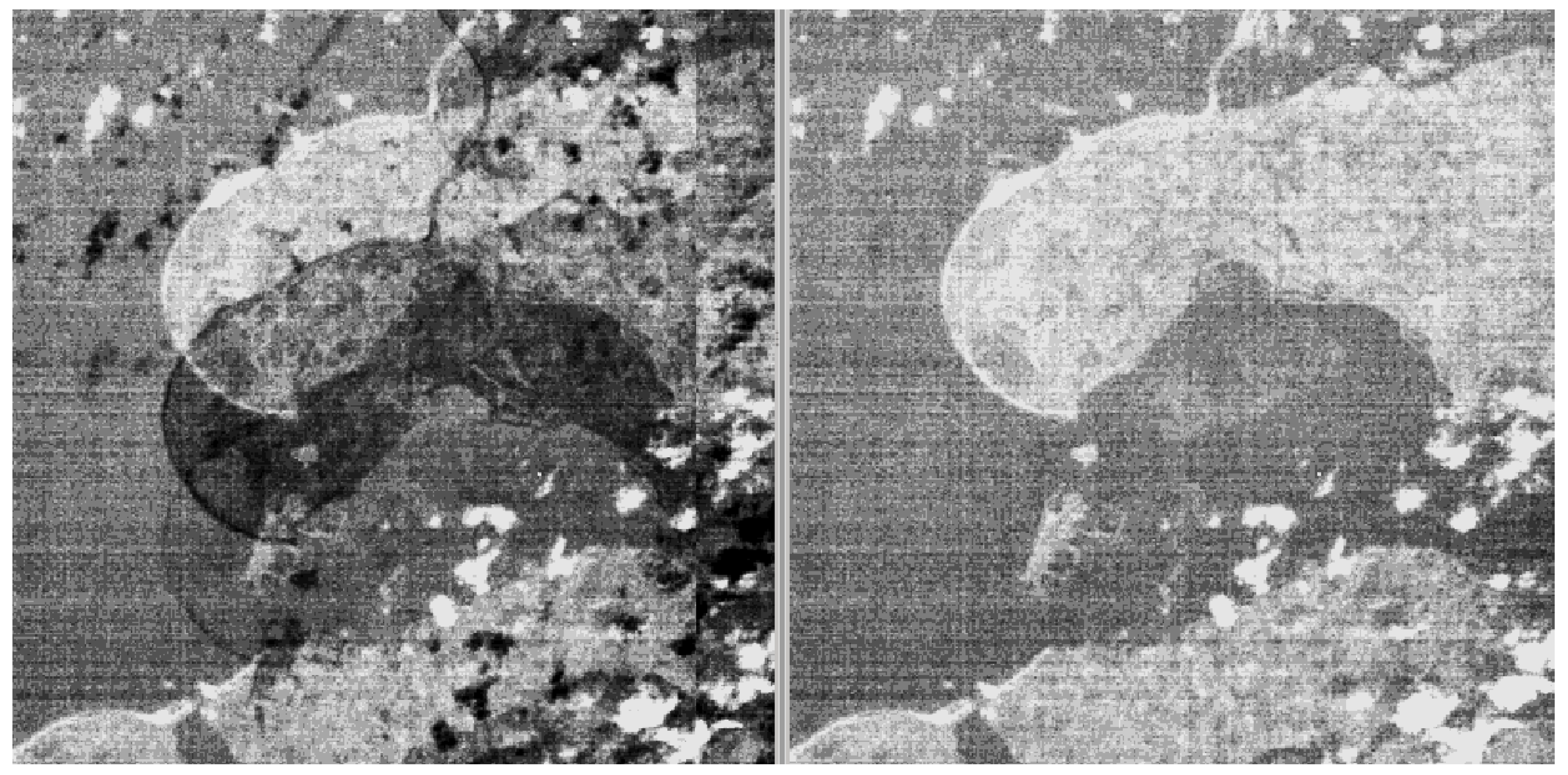
<p><b>Left</b> image shows an example of crosstalk affecting B10 (contrast strongly enhanced). <b>Right</b> represent the corresponding acquisitions in B11 and B12.</p> "> Figure 16
<p>Example of crosstalk correction on band 10 (before/after).</p> "> Figure 17
<p>Overview of the Sentinel-2 GRI selection, July 2016 (European GRI products are not present on this map, since they were produced in the In-Orbit Commissioning Review (IOCR) context, in October 2015).</p> "> Figure 18
<p>Monthly evolution of the image selection for the GRI (April to July 2016).</p> "> Figure 19
<p>Checks from Reference 3D®/BDAmer (turquoise markers) data over Europe. Red and blue lines represent error vector of the product before and after refinement.</p> "> Figure 20
<p>Selection of 33 products over Australia for the GRI.</p> "> Figure 21
<p>Three couples (3 examples over Australia) of homologous points between Sentinel-2 (left) and Australian Geographic Reference Image (AGRI) (right). Each time, the correlation between both images is made at 10m Ground Sample Distance from ground (orthorectified) images.</p> "> Figure 22
<p>Repartition of the Ground Control Points (GCPs) extracted from AGRI.</p> "> Figure 23
<p>Couples of bands used to perform the multi-spectral registration. Blue boxes: 10 m bands; green boxes: 20 m bands; red boxes: 60 m bands.</p> "> Figure 24
<p>Illustration of image equalisation impact: (<b>a</b>) Non-equalised diffuser image; (<b>b</b>) Equalised diffuser image.</p> "> Figure 25
<p>General principle for equalisation assessment.</p> "> Figure 26
<p><b>Left</b>: Sentinel-2 Greenland image from 2015/09/04 together with the 2 uniform zones that are used to estimate the equalization quality. <b>Right</b>: FPN derived independently from the 2 zones.</p> "> Figure 27
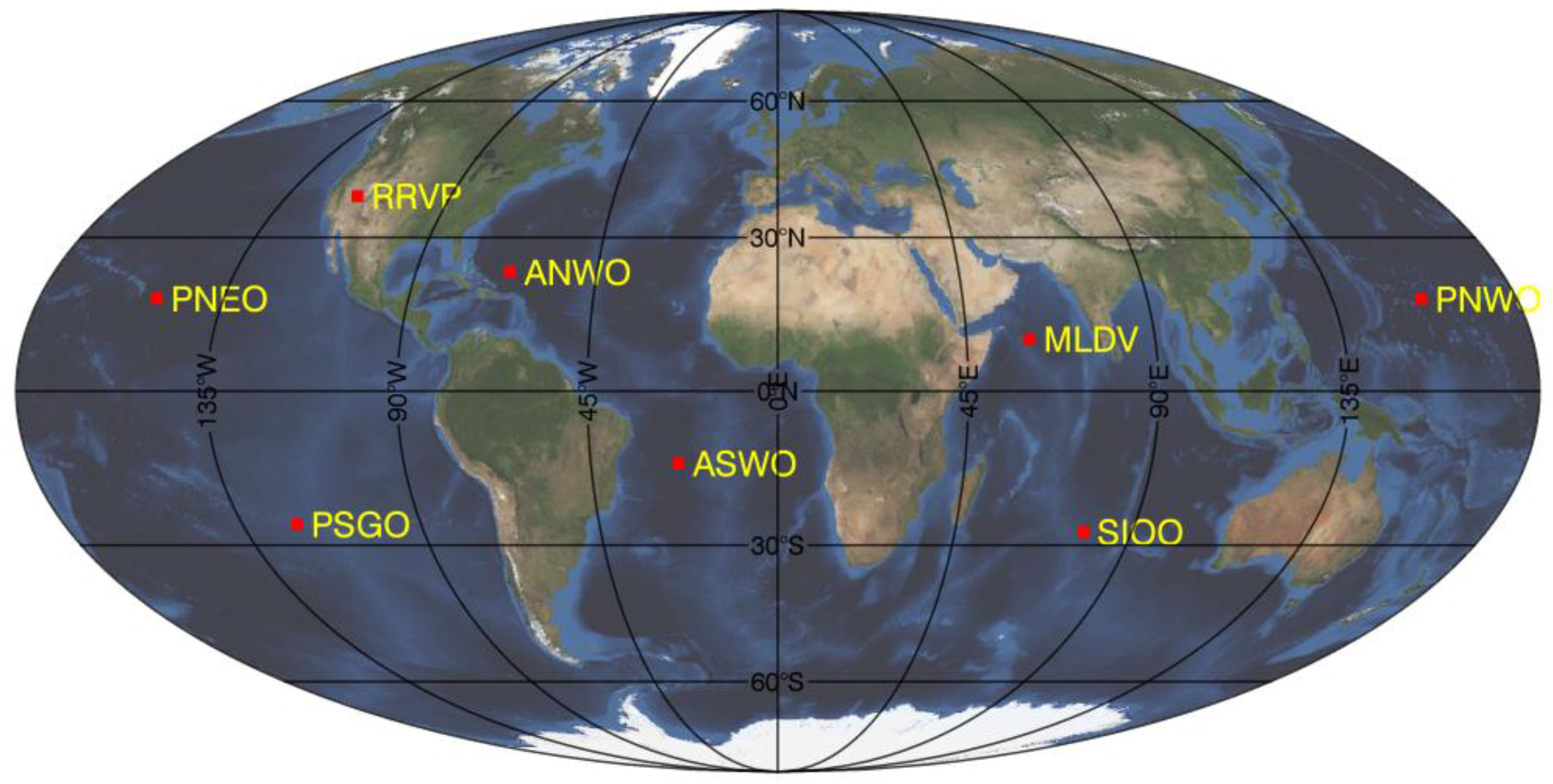
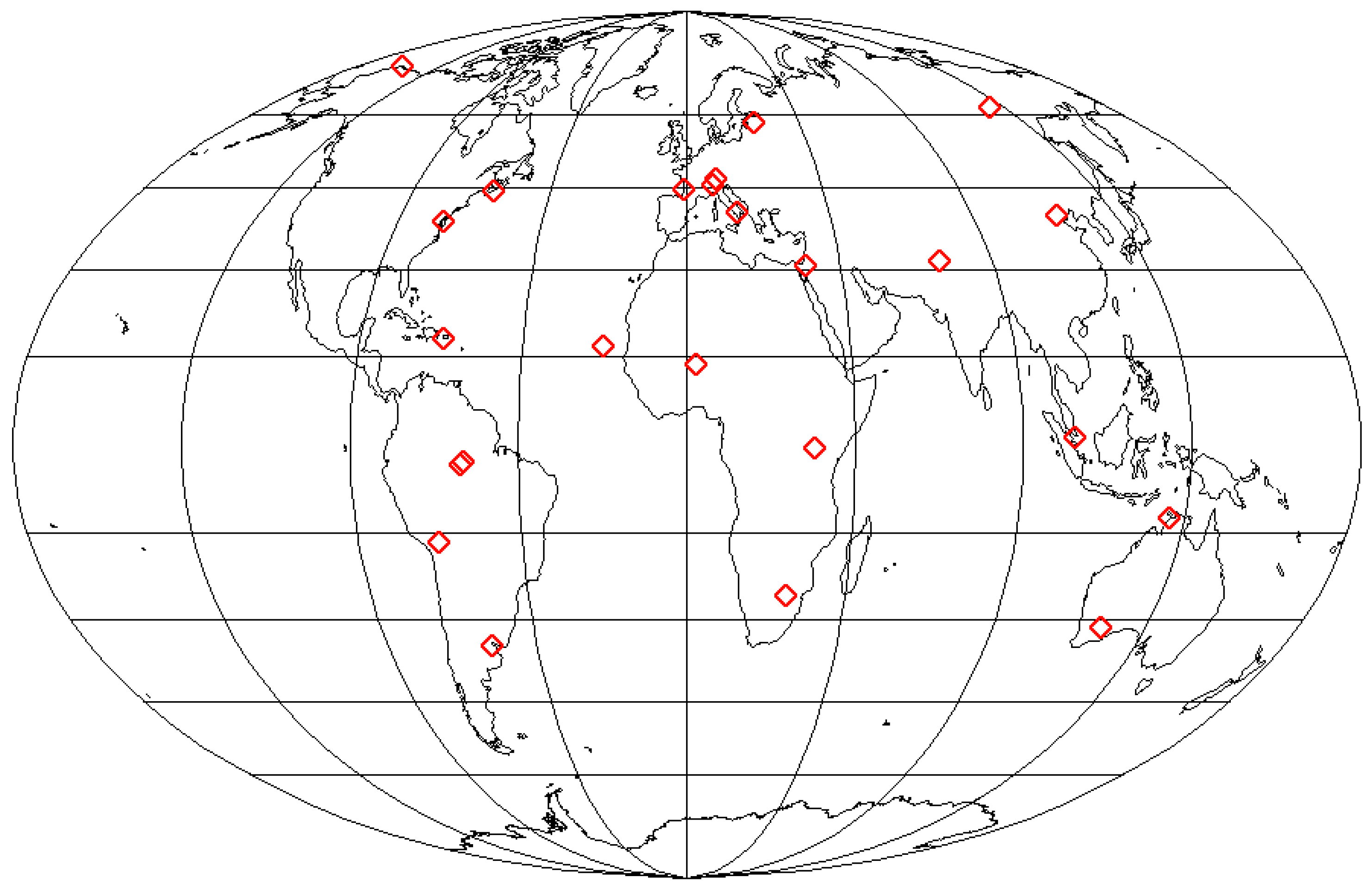
<p>Cal/Val test sites location for Rayleigh scattering, Deep Convective Clouds (DCC), and ground-based methods chosen for Sentinel-2A commissioning activities. ANWO: Atlantic NW-Optimum, ASWO: Atlantic SW-Optimum, PNEO: Pacific NE-Optimum, PNWO: Pacific NW-Optimum, PSGO: Pacific Southern-Gyre-Optimum, SIOO: South-Indian Ocean-Optimum, MLDV: Maldives and RRVP: Rail-Road Valley Playa. (world image is taken from <a href="http://visibleearth.nasa.gov" target="_blank">http://visibleearth.nasa.gov</a>).</p> "> Figure 28
<p>Calibration results over (<b>a</b>) Rayleigh Scattering; (<b>b</b>) ground-based measurements; (<b>c</b>,<b>d</b>) Deep Convective Clouds. The dashed (resp. solid) red lines represent the 3% goal specification (resp. 5% threshold specification). The reference band is B04 and B07 for (<b>c</b>,<b>d</b>) respectively. Error bars indicate the estimated uncertainty for Rayleigh and ground-based measurements and the standard deviation for the DCC method.</p> "> Figure 29
<p>Distribution of valid measurements over DCC sites as a function of detector number. The detector-1 corresponds to the West edge of the swath.</p> "> Figure 30
<p>B01 (<b>left</b>) and B02 (<b>right</b>) inter-band calibration coefficients with respect to B04 as a reference band as a function of the detector number, based on Sentinel-2 images calibrated using the diffuser.</p> "> Figure 31
<p>RGB Quick-Looks from S2A/MSI over (<b>a</b>) Algeria3, (<b>b</b>) Algeria5, (<b>c</b>) Libya1, (<b>d</b>) Libya4, (<b>e</b>) Mauritania1, and (<b>f</b>) Mauritania2 sites. Red squares indicate the region of interest (ROI).</p> "> Figure 32
<p>Time series of TOA reflectance ratio <span class="html-italic">R<sub>b</sub></span> from S2A/MSI over (red) Algeria3, (yellow) Algeria5, (green) Libya1, (light-blue) Lybia4, (dark-blue) Mauritania1 and (purple) Mauritania2 for (from top to bottom) B01, B03, B04 and B8A over the commissioning period. The green (resp. red) dashed lines represent the 5% (resp. 10%) threshold specification. Error bars indicate the estimated uncertainty for the pseudo-invariant calibration sites (PICS) method.</p> "> Figure 32 Cont.
<p>Time series of TOA reflectance ratio <span class="html-italic">R<sub>b</sub></span> from S2A/MSI over (red) Algeria3, (yellow) Algeria5, (green) Libya1, (light-blue) Lybia4, (dark-blue) Mauritania1 and (purple) Mauritania2 for (from top to bottom) B01, B03, B04 and B8A over the commissioning period. The green (resp. red) dashed lines represent the 5% (resp. 10%) threshold specification. Error bars indicate the estimated uncertainty for the pseudo-invariant calibration sites (PICS) method.</p> "> Figure 33
<p>Temporal average of the ratio of observed TOA reflectance to simulated one from S2A/MSI over the four-PICS as a function of wavelength. B05 result is shown with black dashed line due to significant gaseous absorption. The green (resp. red) dashed lines represent the 5% (resp. 10%) threshold specification. Error bars indicate the estimated uncertainty for the PICS method.</p> "> Figure 34
<p>Relative spectral response of (solid-black) S2A/MSI and (dashed-blue) LANDSAT-8/OLI for bands (<b>a</b>–<b>g</b>) 443, 490, 560, 665, 865, 1610 and 2190 nm respectively.</p> "> Figure 35
<p>TOA reflectance ratio defined as S2A-MSI/LS8-OLI measurements derived from extracted doublets over (red asterisk) Algeria3, (orange triangle) Libya4, (blue square) Railroad Valley Playa site (RRVP) and (black diamond) the average over the three test sites as a function of the wavelength. The green (resp. red) dashed lines represent the 5% (resp. 10%) threshold specification. Error bars indicate the estimated uncertainty.</p> "> Figure 36
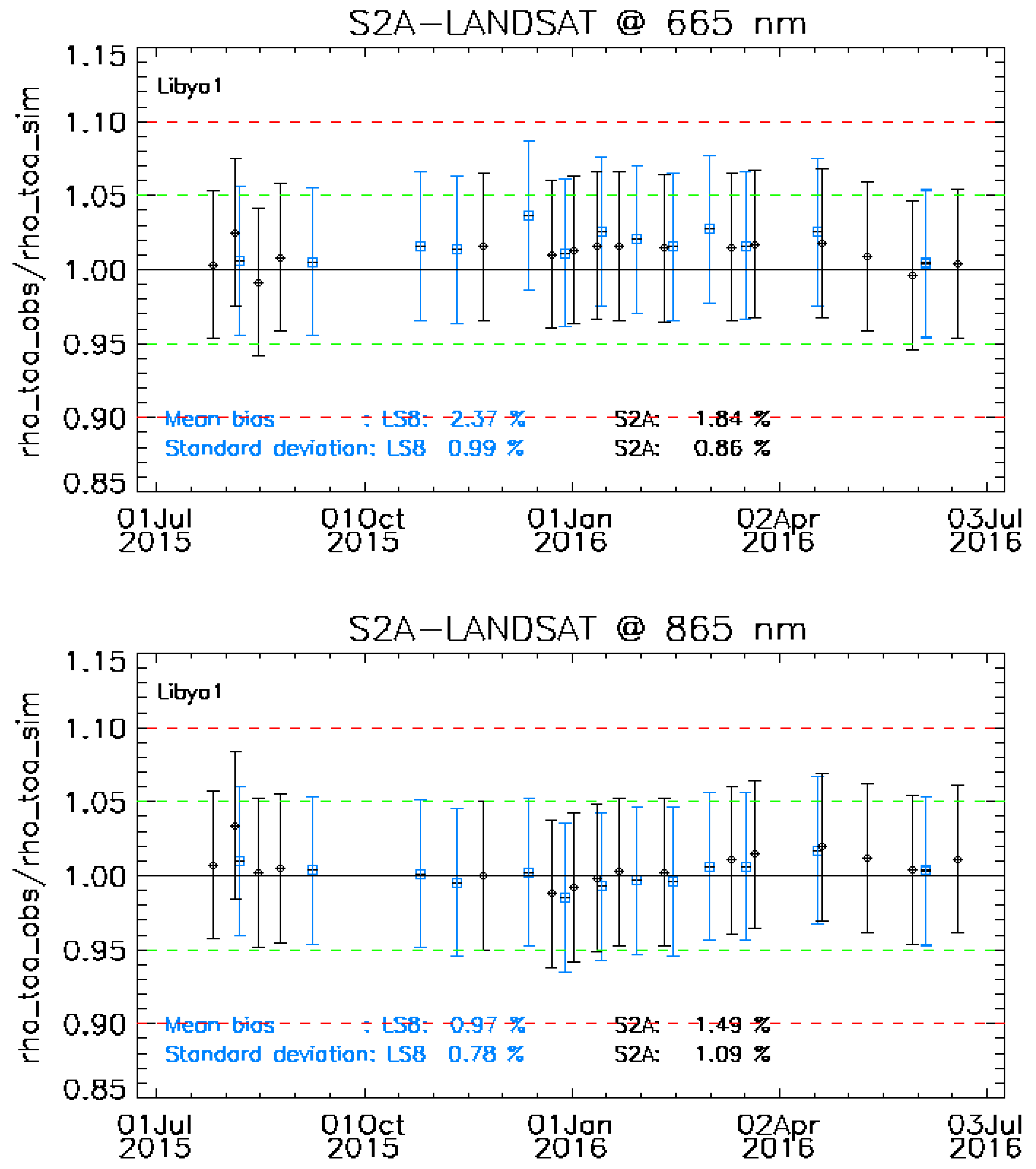
<p>Time series of TOA reflectance ratio R<sub>b</sub> from (black) S2A/MSI and (blue) LS8/OLI over Lybia1 for (from top to bottom) B03, B04 and B8A from S2A over the commissioning period. The green (resp. red) dashed lines represent the 5% (resp. 10%) threshold specification. Error bars indicate the estimated uncertainty for the PICS method.</p> "> Figure 36 Cont.
<p>Time series of TOA reflectance ratio R<sub>b</sub> from (black) S2A/MSI and (blue) LS8/OLI over Lybia1 for (from top to bottom) B03, B04 and B8A from S2A over the commissioning period. The green (resp. red) dashed lines represent the 5% (resp. 10%) threshold specification. Error bars indicate the estimated uncertainty for the PICS method.</p> "> Figure 37
<p>Ratio of observed TOA reflectance to simulated one for each sensor (black) S2A/MSI and (blue) LANDSAT-8/Operational Land Imager (OLI) over Algeria3, Libya1, Libya4, and Mauritania2 sites as a function of wavelength. The green (resp. red) dashed lines represent the 5% (resp. 10%) threshold specification. Error bars indicate the estimated uncertainty for the PICS method.</p> "> Figure 37 Cont.
<p>Ratio of observed TOA reflectance to simulated one for each sensor (black) S2A/MSI and (blue) LANDSAT-8/Operational Land Imager (OLI) over Algeria3, Libya1, Libya4, and Mauritania2 sites as a function of wavelength. The green (resp. red) dashed lines represent the 5% (resp. 10%) threshold specification. Error bars indicate the estimated uncertainty for the PICS method.</p> "> Figure 38
<p>Sentinel-2 reference radiance L<sub>ref</sub> (W/m²/sr/μm), Signal-to-Noise Ratio (SNR) requirement at reference radiance and current SNR measurement on sun-diffuser at reference radiance.</p> "> Figure 39
<p>Average SNR at reference radiance L<sub>ref</sub> measurements (per band) since January 2016.</p> "> Figure 40
<p>Modulation Transfer Function (MTF) curve for B02 band (centred at 490 nm) for the across-track direction.</p> "> Figure 41
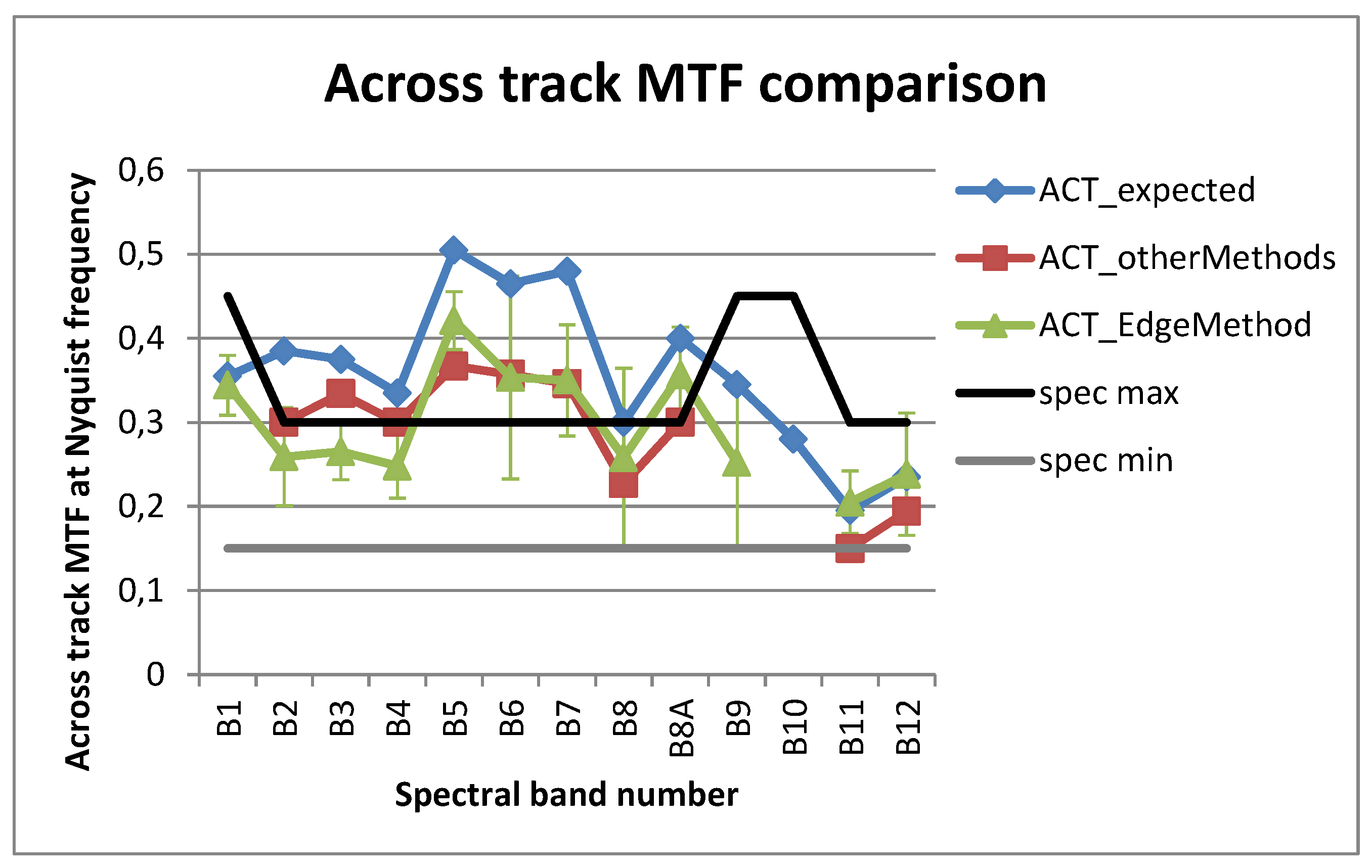
<p>MTF results for the across-track direction, and MTF requirements (min value, spec min and max value, spec max).</p> "> Figure 42
<p>MTF results for the along-track direction, and MTF requirements (min value, spec min and max value, spec max).</p> "> Figure 43
<p>General principle of geolocation uncertainty validation using ground control points. Mean shift computation is obtained by correlation technique.</p> "> Figure 44
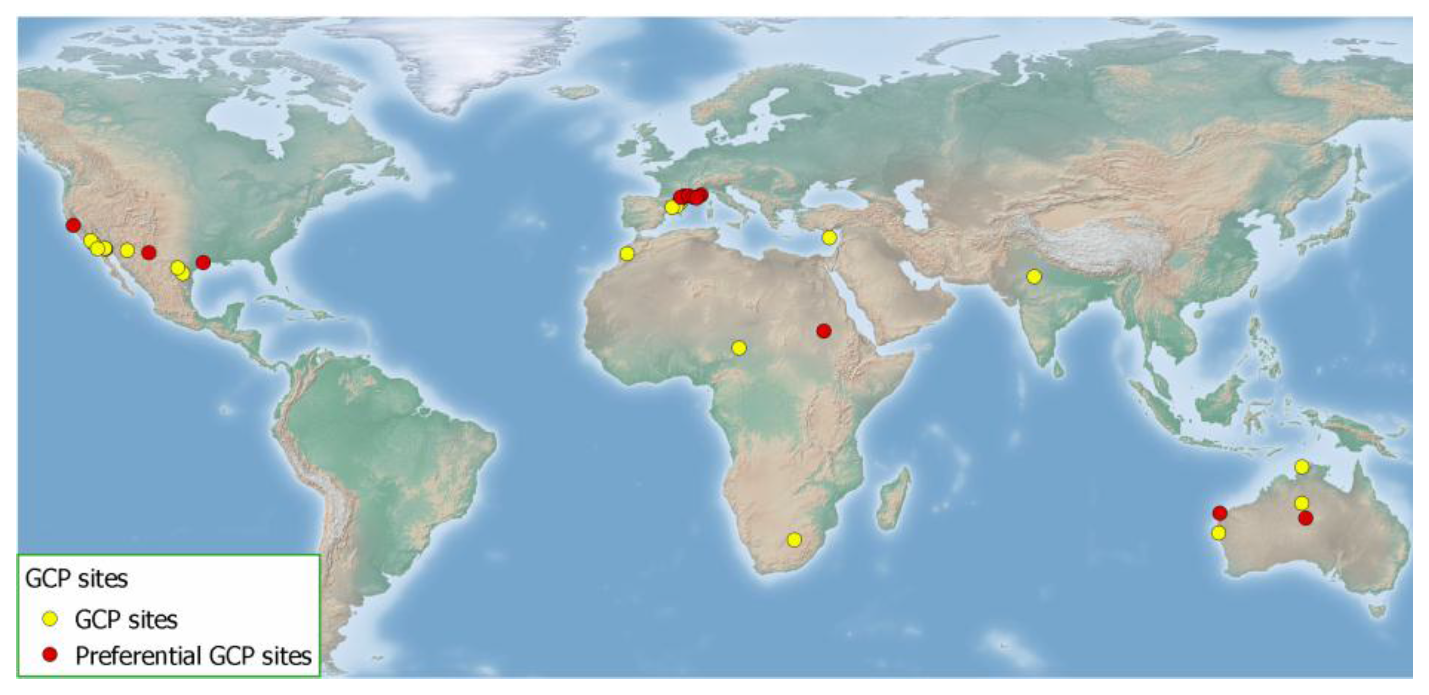
<p>Map of Thale Alenia Space GCP database sites (red dots are GCP sites currently available and used as baseline for S2 validation activities).</p> "> Figure 45
<p>System Geolocation Performances in metres (Band 04) for L1B non-refined products. Red (resp. orange) circle is the requirement without (res. with) geometric refinement on GCPs.</p> "> Figure 46
<p>System Geolocation Performances in metres for L1C non-refined products. Reference band is B04. (<b>a</b>) Geolocation error (in metre) along-track and across-track measured on each GCP; (<b>b</b>) Mean geolocation error in each product processed in function of the acquisition dates of the product. The two outliers seen on both figures correspond to products from orbit 5601 and are due to contingencies (star-tracker outage).</p> "> Figure 47
<p>Product Geolocation Performances in metres (Band 04) for L1C refined tiles. Orange circle is the requirement with geometric refinement on GCPs.</p> "> Figure 48
<p>High-level principle of the multi-spectral registration uncertainty assessment.</p> "> Figure 49
<p>Example of global mis-registration shifts measured on ‘Central Australia’ for B04/B03-Detector 08 and B05/B12-Detector 02. Black points are tie points rejected based on correlation quality criteria (step 4). Units are pixels of the coarser band in the couple.</p> "> Figure 50
<p>High-level principle of the multi-temporal registration uncertainty assessment.</p> "> Figure 51
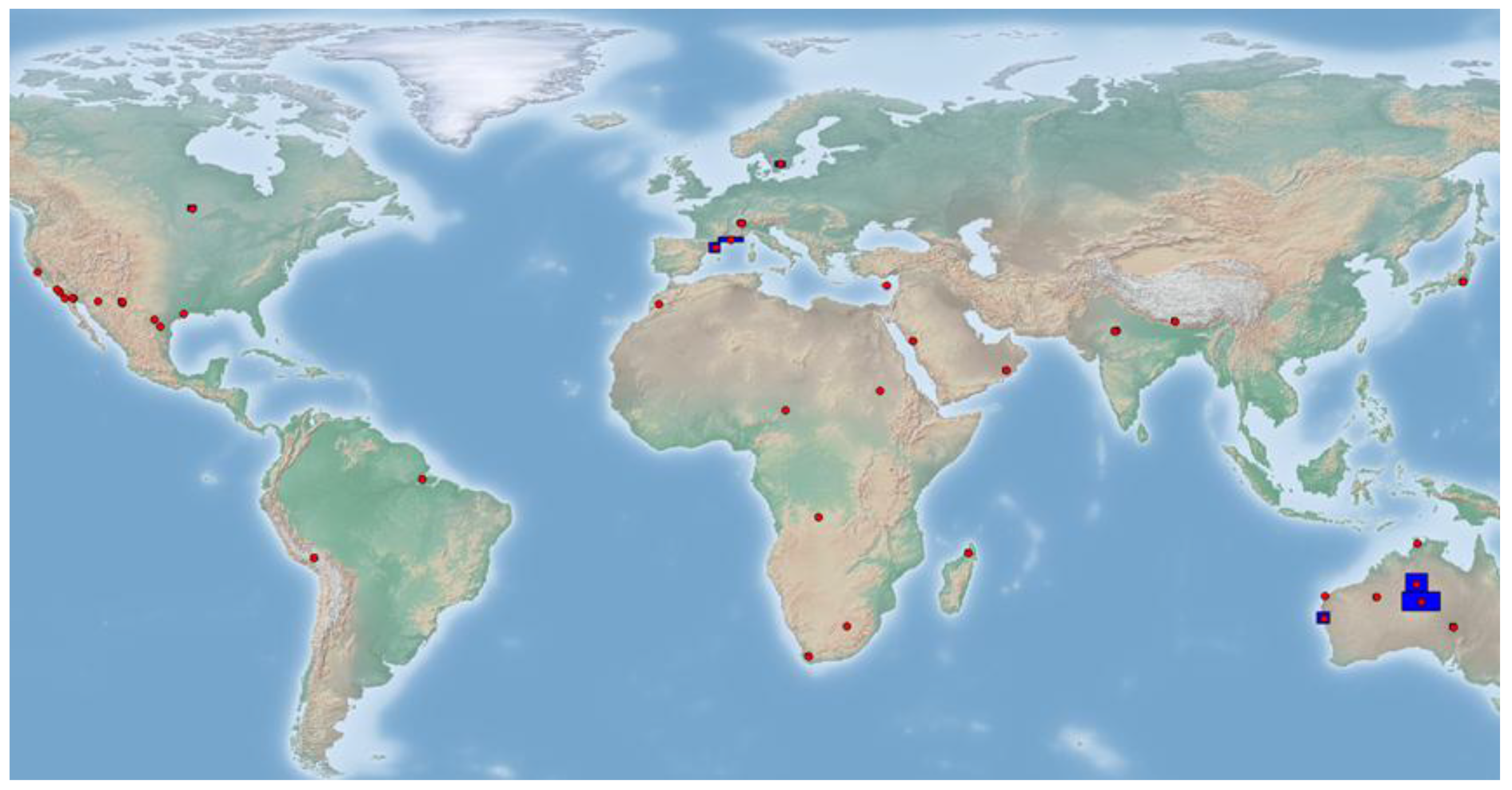
<p>Sites used for multi-temporal registration uncertainty validation on non-refined products (red points). They include the geolocation validation sites (in blue) and other sites specific for multi-temporal registration assessment.</p> "> Figure 52
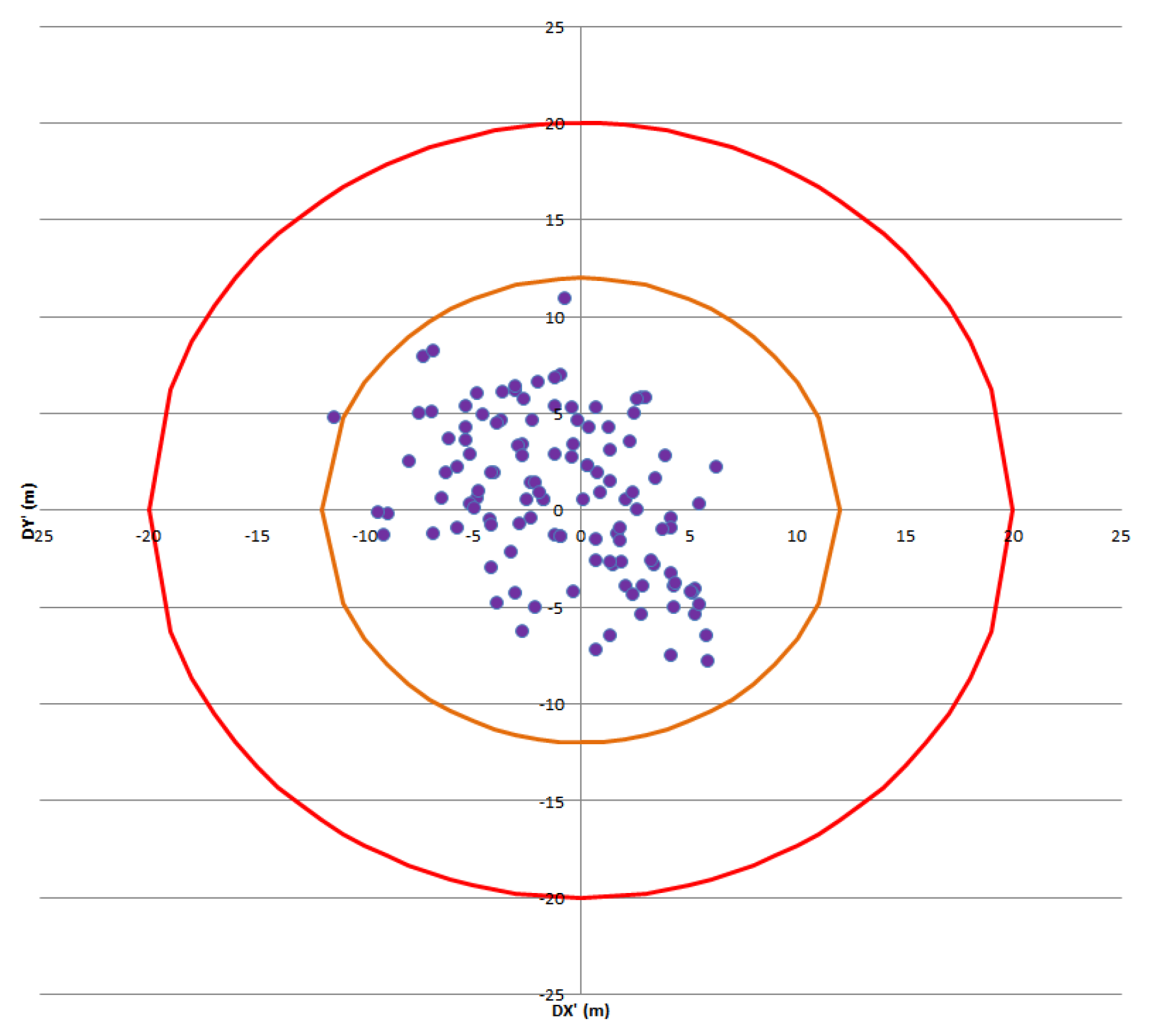
<p>Multi-temporal registration uncertainty. Each point represents the average X shift and Y shift measure in one secondary tile with respect to the reference tile.</p> "> Figure 53
<p>Areas used for multi-temporal registration uncertainty validation on refined products.</p> "> Figure 54
<p>Multi-temporal (XT) registration uncertainty for B04 band. Each point represents the average shift measured in one secondary tile with respect to the reference tile.</p> "> Figure 55
<p>Multi-temporal (XT) registration uncertainty for B11 band. Each point represents the average shift measured in one secondary tile with respect to the reference tile.</p> "> Figure 56
<p>Coverage percentage of Europe GRI versus relative orbit number.</p> "> Figure 57
<p>European GRI product strips according to Pleiades references.</p> "> Figure 58
<p>European GRI product geolocation performance.</p> "> Figure 59
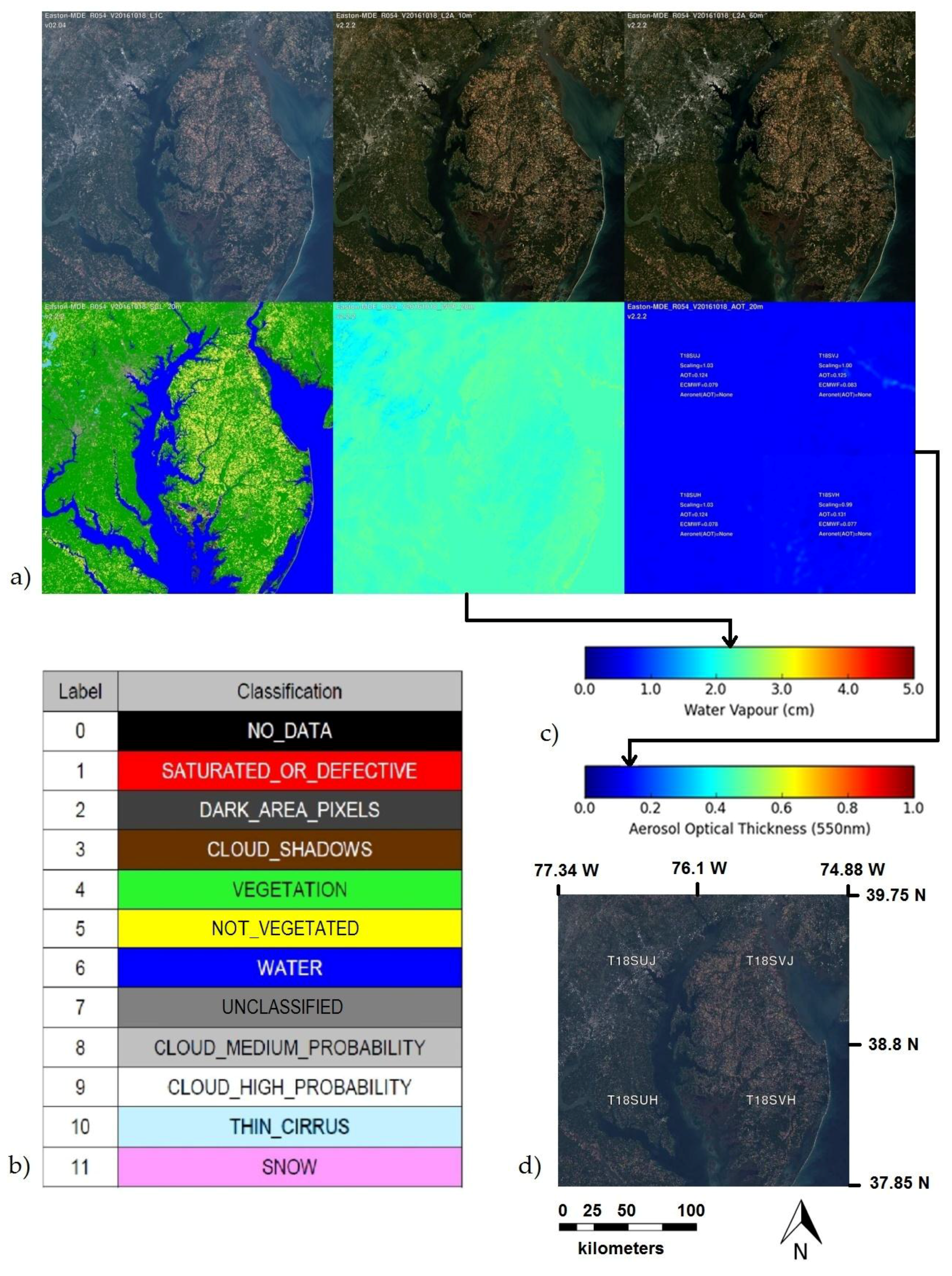
<p>(<b>a</b>) Level-2A product example. Aeronet site Easton-Maryland-Department-Environment (USA), acquired on October 18, 2016, characterized by MidlatitudeN, Flat terrain, Forest, Croplands, Water, Urban. (Top) RGB compositions (B04, B03, B02) for L1C TOA, L2A Surface Reflectance (SR) at 10 m, L2A SR at 60 m; (Bottom) Scene Classification, L2A Water Vapour at 20 m, L2A Aerosol Optical Thickness (AOT) at 20 m. (<b>b</b>) Cloud Screening and Scene Classification (SCL) pixel legend; (<b>c</b>) Colour tables for Total Water Vapour Column and Aerosol Optical Thickness at 550 nm; (<b>d</b>) Scale, north arrow and coordinates of the four product granules.</p> "> Figure 60
<p>Geographical distribution of the 24 selected AERONET test sites for the Level-2A Calibration.</p> "> Figure 61
<p>(<b>a</b>) Cloud shadows classification; (<b>b</b>) Topographic shadows classification.</p> "> Figure 62
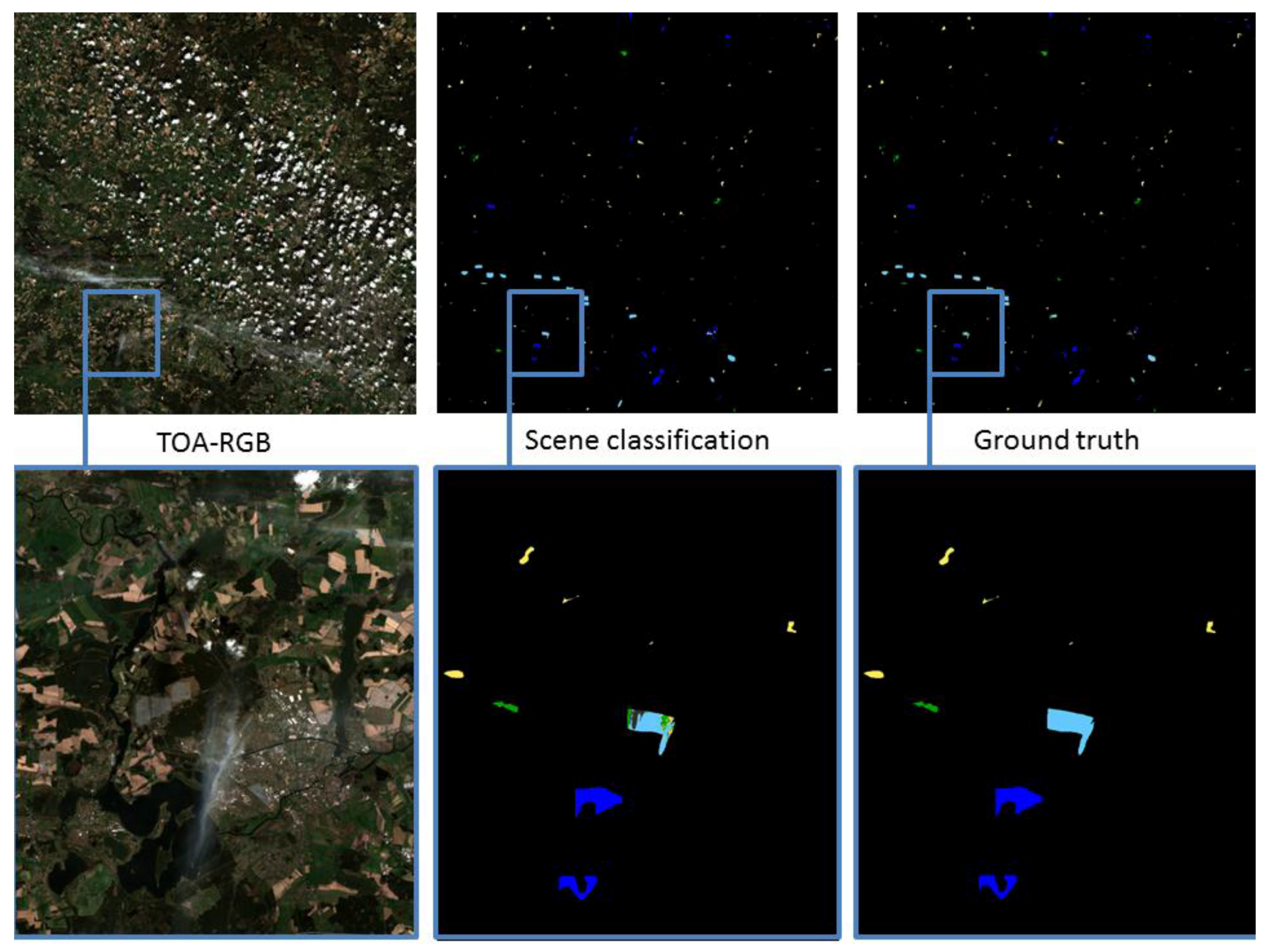
<p>Example images for Cloud Screening and Classification Validation analysis, Site Potsdam (Germany), acquired on April 22, 2016, characterized by temperate climate zone and flat terrain. Whole granule at the top and zoomed area at the bottom.</p> "> Figure 63
<p>AOT and Water Vapour (WV) Validation. Direct comparison of Sen2Cor with ground reference from AERONET. Sen2Cor is represented by average over 9 km × 9 km area with AERONET sunphotometer in the centre. Filled symbols represent samples with cloudiness >5% and not filled with cloudiness <5%.</p> "> Figure 64
<p>Validation example for Bottom-Of-Atmosphere (BOA) reflectance, Site Belsk (Poland), acquired on 14th of August 2015, characterized by flat terrain. (<b>Left</b>): BOA-RGB and scene classification image of the 9 × 9 km<sup>2</sup> area around AERONET sunphotometer (longitude 20.79 E, latitude 51.84 N). (<b>Right</b>): Example spectra and relative difference to reference for soil and vegetated pixels at indicated locations.</p> ">
Abstract
:1. Introduction
2. Multi-Spectral Instrument Overview
2.1. MSI Design
2.2. Spectral Bands and Resolution
- 4 bands at 10 m spatial resolution: blue (490 nm), green (560 nm), red (665 nm) and near infrared (842 nm).
- 6 bands at 20 m spatial resolution: 4 narrow bands mainly used for vegetation characterization in the red edge (705 nm, 740 nm, 783 nm and 865 nm) and 2 wider SWIR bands (1610 nm and 2190 nm) for applications such as snow/ice/cloud detection or vegetation moisture stress assessment.
- 3 bands at 60 m spatial resolution for applications such as cloud screening and atmospheric corrections (443 nm for aerosols, 945 nm for water vapour and 1375 nm for cirrus detection).
2.3. Focal Plane Layout—Pixels Line of Sight
2.4. Detector Specificities
2.5. On-Board Equalization and Compression
2.6. On-Board Sun Diffuser
3. Products Overview
3.1. Processing Levels
- Level-0 (L0) products: Raw instrument data packaged for long-term storage and future reprocessing campaigns. A coarse cloud mask is appended for cataloguing purposes.
- Level-1A (L1A) products: Uncompressed instrument data in sensor geometry and with a coarse registration (i.e., rough pixel alignment between images from different spectral bands and detector modules). No resampling nor radiometric corrections have been applied. These products are used for calibration purposes.
- Level-1B (L1B) products: Top-Of-Atmosphere (TOA) radiances in sensor geometry (same as Level-1A products). Full radiometric corrections have been applied. These products are used for calibration, validation and quality control purposes.
- Level-1C (L1C) products: TOA reflectances in cartographic geometry. These products are publicly disseminated by ESA.
- Level-2A (L2A) products: Bottom-Of-Atmosphere (BOA) reflectances in cartographic geometry (same as Level-1C products). Today, these products can be generated by users with the publicly available Sen2Cor processor. L2A production is now systematic over Europe and dissemination through the Copernicus Open Access Hub [6] started in May 2017.
3.2. Level-1 Processing Steps
3.3. Level-2A Processing Steps
3.4. Level-1C Product Description
3.5. Level-2A Products Description
- Surface (or BOA) reflectance images which are provided at different spatial resolutions (60 m, 20 m and 10 m);
- Aerosol Optical Thickness (AOT) and Water Vapour (WV) maps (60 m, 20 m and 10 m);
- Scene Classification (SCL) map used internally as input for atmospheric correction together with Quality Indicators for cloud and snow probabilities (60 m and 20 m).
3.6. Processing Baseline Evolutions
4. Level-1 Calibration and Validation Status
4.1. Radiometry Calibration Activities
4.1.1 Dark Signal Calibration
4.1.2. Absolute Radiometric Calibration
4.1.3. Relative Gains Calibration
4.1.4. SWIR Detectors Re-Arrangement Parameters Generation
- 1: valid pixel with SNR compliant to specification,
- 2: valid pixel with SNR below specification,
- 3: non-valid saturated pixel,
- 4: non-valid blind pixel,
- 5: non-valid with SNR below specification.
4.1.5. Crosstalk Correction Calibration
- Region 1: the signal is the signal measured in B10 far from the lake from which is subtracted 0.45% of the signal measured in B11 (around 5 DC) and 0.2% of the signal measured in B12 (around 2 DC) also far from the lake. B10 own signal is a landscape residual that is seen because of the lack of cirrus.
- Region 2: B10 is on the lake. B10 own radiometry is around 0 DC but B11 and B12 are not yet on the lake and crosstalk induces negatives values at focal plane level on B10. At ground level those negative values are truncated to zero.
- Region 3: B10 is still on the lake. B11 is now on the lake but B12 not yet. Thus the radiometry is superior to the one observed in region 2 because B11 crosstalk is null (because B11 radiometry is null).
- Region 4: B10, B11 and B12 are on the lake. Crosstalk is negligible. On this region we observe the real response of B10 on the lake.
- Region 5: B10 is no more on the lake but B11 and B12 are still. On this region we observe the real response of B10 on the lake border.
- Region 6: B10 and B11 are no more on the lake. B12 is still on the lake.
- Region 7: idem region 1.
4.1.6. MSI Refocusing
4.2. Geometric Calibration Activities
4.2.1. Global Reference Image Generation
4.2.1.1. Definition and Goals of the Global Reference Image
- The geolocation of L1C products refined with the GRI is better than 12.5 m CE95 (95 percentile of the circular error).
- The multi-temporal registration performance between refined products is better than 0.3 pixels.
4.2.1.2. Selection and Constitution
4.2.1.3. Methods of Refinement
- Identification on ground calibration sites or ITRF GPS network: the ITRF (International Terrestrial Reference Frame) network is worldwide. When possible, GCPs from these sites are used.
- Identification in an image of reference: several sources can be used as a reference because they are accurate enough for GRI need. This is the case of aerial BD Ortho ® over France made by IGN, AGRI (Australian Geographic Reference Image) made with ALOS imagery over Australia, aerial imagery over the USA made by the USGS, etc. In this use case, homologous points of interest are extracted between the reference and the GRI to be built. This extraction is done automatically or manually when the automatic process fails.
4.2.1.4. Internal Controls
4.2.1.5. The Example of Australia
4.2.2. Absolute and Relative Calibration of the Focal Plane
4.2.2.1. Methods
- B4 spectral band is used as a reference to calibrate the focal plane of the B2, B3, B5 and B8 spectral bands;
- B5 spectral band is used as a reference to calibrate the focal plane of the B1, B6, B7, B11 and B12 spectral bands;
- B8 spectral band is used as a reference to calibrate the focal plane of the B8a and B9 spectral bands;
- B2 spectral band is used as a reference to calibrate the focal plane of the B10 spectral band.
4.2.2.2. Results
- products are located anywhere around the world so cloud-free acquisitions can be chosen;
- correlation is computed between two Sentinel-2 products: a reference image is not needed as the correlation noise is low.
- Static LOS calibration residuals;
- Dynamic vibrations residuals that represent the main contributor because of on-board oscillations;
- Correlation noise and outliers which depend on landscapes and spectral couples.
4.2.3. Absolute Calibration of the Viewing Frames
4.2.3.1. Methods
- Determine any possible change in alignment biases as a function of criteria such as latitude (analysis of possible thermo-elastic effects),
- Avoid being too dependent on weather conditions.
- Determine a mean biases set to update GIPP,
- Observe a possible evolution of biases according to such criteria as latitude, date, etc.
4.2.3.2. Results
4.3. Radiometry Validation Activities
4.3.1. Equalisation Validation
4.3.1.1. Methods
- On-board Sun-diffuser acquisitions: in this case the true radiance is known;
- “Uniform” natural targets on Earth (vicarious method): deserts, ice, etc.
- (1)
- For each detector, correct each pixel of the sun-diffuser BRDF (to avoid local fluctuations due to the spatial response of the sun-diffuser) and of solar angle: Compute the average line of the ratio between observed radiance and sun-diffuser simulated radiance (see Equation (3) in Section 4.1.2):In practice the average is computed over Nl = 5000 lines (at 10 m resolution).
- (2)
- Build a full-swath line concatenating the previous average line but keeping only pixels that will be seen in the end-user product: R(b,p’)
- (3)
- Using a sliding window with a step of 1 pixel, compute the mean and standard deviations over a section of 100 pixels and derive the (normalised) FPN and MEN:
- , where MEAN and STD are respectively mean and standard-deviation over pixels in the sliding window centred at p.
- over all pixels across-track
- (1)
- Compute the mean line of the image.
- (2)
- Compute FPN and MEN performing step (3) of the method using sun-diffuser acquisitions.
4.3.1.2. Results on Sun-diffuser Acquisitions
4.3.1.3. Results on Uniform Scenes
4.3.2. Absolute Radiometry Vicarious Validation
4.3.2.1. Methods
4.3.2.1.1. Rayleigh Scattering Over Ocean Surface
4.3.2.1.2. Inter-Band Calibration over Deep Convective Clouds
- is the radiance at top of the cloud, which depends on the geometrical conditions, the cloud particle type and, less significantly, on what is under the cloud (aerosols, tropospheric molecular signal, etc.). The clouds are so thick that the surface has zero influence on the result.
- is the residual molecular signal over the cloud.
- is the residual aerosol signal over the cloud.
- is the gaseous transmission above the cloud.
4.3.2.1.3. Ground-Based Reflectance Measurements
4.3.2.2. Results and Analysis
4.3.2.2.1. Rayleigh Scattering Results
4.3.2.2.2. Deep Convective Clouds Method Results
4.3.2.2.3. Ground-Based Reflectance Measurements Results
4.3.3. Multi-Temporal Relative Radiometry Vicarious Validation
4.3.3.1. Pseudo-Invariant Calibration Site Methodology
4.3.3.2. Sites Selection
4.3.3.3 Results and Analysis
4.3.4. Absolute Radiometry Cross-Mission Inter-Comparison
4.3.4.1. Methods
4.3.4.1.1. Sensor-to-Sensor Inter-Calibration
4.3.4.1.2. Pseudo-Invariant Calibration Site Methodology
4.3.4.2. Results and Analysis
4.3.4.2.1. Sensor-to-Sensor Inter-Calibration Results
4.3.4.2.2. PICS Methodology Results
4.3.5. Inter-band Relative Radiometric Uncertainty Validation
4.3.5.1. Method and Outlook
4.3.6. Signal-to-Noise Validation
4.3.6.1. Method
- is the radiometric noise standard-deviation (in W/m²/sr/μm).
- L is the radiance (in W/m2/sr/μm).
- and are the noise model parameters, both in in W/m²/sr/μm.
- ◦
- represents the dark noise standard-deviation (at radiance 0).
- ◦
- βL·L represents the variance of the shot noise (due to the particle nature of light) at radiance L.
- is directly determined from measurement of noise standard-deviation on a dark image (L ≈ 0).
- is determined from measurement of noise standard-deviation in a sun-diffuser image and by inversion of Equation (14) using the knowledge (from diffuser model) of diffuser radiance and current estimation of αL.
- On dark image:◦ on dark image is simply the standard-deviation of the radiance levels in one column.
- On sun-diffuser image:◦ on sun-diffuser image is the standard-deviation of the radiance levels in one column corrected from the sun-diffuser non-uniformity (BRDF and solar angles effects) known from sun-diffuser simulated radiance (see Equation (2) in paragraph 4.1.2).
4.3.6.2. Results
4.3.7. Modulation Transfer Function Validation
4.3.7.1. Methods
- x varies along the line of the image,
- y varies along the row of the image,
- h is the impulse response in other words the Point Spread Function (PSF),
- The DiracComb corresponds to the sampling by the detectors in the focal plane,
- * is the convolution product,
- . is the multiplication.
- fx is the spatial frequency for the line (or across-track) direction,
- fy is the spatial frequency for the row (or along-track) direction,
- H is the Transfer Function.
- Choosing a landscape so that the term LandscapeSpectrum can be known,
- Managing the replication in order to avoid aliasing effect that corresponds to mixing, for some frequency range, of the pattern with its replica.
4.3.7.1.1. Reference Image Method
4.3.7.1.2. Bridge Method
4.3.7.1.3. Edge Method
4.3.7.2. Results
4.4. Geometry Validation Activities
4.4.1. Geolocation Uncertainty Validation
4.4.1.1. General Methods and Data
- (1)
- Find approximate GCP location in Sentinel 2 image using product geolocation metadata (L1B physical geolocation model or L1C georeferencing metadata).
- (2)
- Resample both images in the same geometry: Either S2 image is resampled to GCP image or GCP image is resampled to Sentinel 2 image. This is based on L1B physical geolocation model or L1C georeferencing metadata.
- (3)
- Assess the GCP geolocation error (shift between the GCP image and Sentinel-2 image) by correlation technique.
- (4)
- Repeat the previous steps for several GCPs in one product and several products.
- (5)
- Filter out bad correlation points based on correlation quality criteria
- (6)
- Compute statistics to assess performance (e.g., at 95.45% confidence level).
- A dedicated high-resolution ortho-images database with geolocation accuracy better than 5m is used by Thales Alenia Space in the frame of MPC, see world distribution in Figure 44.
- Pleiades HR database including more than 500 images with accuracy better than 5 m is used by CNES.
- the accuracy of matching algorithm, given the difference in acquisition date, sensors characteristics and acquisition conditions between Sentinel-2 images and the reference image,
- the number of GCPs and their distribution over the scene.
- In step (2) GCPs ortho-images (in any cartographic projection) are resampled onto Sentinel-2 L1C tile cartographic projection.
- The error shifts are thus observed in fraction of L1C pixels directly convertible into meters or X/Y UTM coordinates. The shifts can be converted into across-track and along-track directions using knowledge of satellite acquisition direction on ground.
- (1)
- For each processed S2 product, compute the mean circular error on all GCPs inside the product.
- (2)
- Compute the quantile at 95.45% of the mean circular errors over all the products.
4.4.1.1.1. Results for Non-Refined Products
4.4.1.1.2. Results for Refined Products
4.4.2. Multi-spectral Registration Uncertainty Validation
- System level, on L1B products without any improvement of VIS/SWIR focal planes registration by processing task.
- Product level, on L1B products with focal plane registration processing between VNIR and SWIR focal planes enabled. In that case the registration within each focal plane is not refined and the performance is the same as system level performance.
4.4.2.1. Methods
- (1)
- Resample the image with the finest resolution (secondary image) in the geometry of the image with the coarsest resolution (reference image). For that purpose a resampling grid establishing the correspondence between pixels of the reference band and their position in the secondary band is computed using the line of sights physical model. Then a B-spline interpolation method is used to interpolate the radiometric values of the secondary band at locations defined by the resampling grid.
- (2)
- Select a list of well-matching tie-points in the images where to perform the correlations (avoiding clouds, water, etc) and extract small image chips around tie-points in both images.
- (3)
- This process is applied to cloud-free products acquired on several areas at different latitudes and with various kinds of landscapes to estimate registration uncertainty (along-track and across-track shifts) at each tie point by correlation of the reference and secondary image chips.
- (4)
- Filter out outliers with poor correlation based on correlation quality criteria
- (5)
- Compute the registration uncertainty parameter: 99.73% quantile among shifts measured on all tie-points. This is compared to the requirement.
- (6)
- Compare results against requirements.
4.4.2.2. Results
4.4.3. Multi-Temporal (XT) Registration Uncertainty Validation
- The current multi-temporal registration performance for non-refined product which is representative of the current situation.
- A preliminary assessment of the performance with refinement activated, based on products processed with the ground-processor prototype and the available European part of the GRI.
4.4.3.1. Method
- (1)
- Select two cloud-free L1C tiles acquired on the same area on Earth at different dates. Select also the reference band to be processed. In practice, for a given tile, the older L1C image is taken as reference and all new cloud-free acquisitions of the same tile are compared to the reference tile.
- (2)
- Select a list of well-matching tie-points in the images where to perform the correlations (avoiding clouds, water, etc.) and extract small image chips around tie-points in both images.
- (3)
- Estimate registration uncertainty (shifts along X and Y axes) at each tie point by correlation of the reference and secondary image chips.
- (4)
- Filter out outliers with poor correlation based on correlation quality criteria.
- (5)
- Compute the registration uncertainty metrics at tile level: Average circular error over all non-rejected tie-points of the tile.
- (6)
- Repeat the previous steps (1) to (5) for as many tile couples as possible.
- (7)
- Compute the global registration uncertainty metrics, to be compared to the requirement: 95.45% quantile among the average shifts measured on each L1C tile couples.
- The quality of the images,
- The seasonal scene variations and meteorological/atmospheric properties (water vapour and aerosols should be limited in the processed scenes),
- The properties of the scene, relief, surface reflectance, and image content,
- When the two tiles correlated have been acquired from two adjacent orbits (i.e. covering the overlapping areas), the viewing angles are different. In areas with relief this causes a parallax between the two images that can degrade the correlation accuracy.
4.4.3.2. Results for Non-Refined Products
4.4.3.3. Results for Refined Products over European GRI
- Orbit 51: 6 dates, 312 tiles (France).
- Orbit 50: 6 dates, 76 tiles (East Europe).
- Orbit 35: 4 dates, 48 tiles (Middle East).
- Orbit 137: 2 dates, 12 tiles (UK).
- Orbit 122: 2 dates, 10 tiles (Austria).
- Orbit 36: 3 dates, 12 tiles (Hungary).
- Orbit 22: 4 dates, 8 tiles (Sweden).
- Orbit 64: 2 dates, 27 tiles (Ukraine).
4.4.4. Global Reference Images Validation
4.4.4.1. Methods
4.4.4.2. Results for European Block of Global Reference Image
- Orbit 021: 1240 km missing on the North.
- Orbit 035: 1600 km missing on the North.
- Orbit 078: 1100 km missing on the North.
- Green: more than 6 Pleiades references crossing. The computed location precision will be very reliable.
- Orange: 3 to 5 Pleiades references crossing
- Red: 1 or 2 Pleiades references crossing
- Black: no Pleiades references crossing. The location performance cannot be computed for these products.
- Green: geolocation better than 7 m.
- Orange: geolocation between 7 m and 10 m.
- Red: geolocation worse than 10 m.
- Black: no reference to estimate geolocation.
- White: missing products in the final GRI.
5. Level-2A Calibration and Validation Status
5.1. Level-2A Calibration Activities
5.1.1. Level-2A Calibration Dataset
5.1.2. Atmospheric Correction Parameterization
5.1.2.1. Method
- The sensitivity of the Sen2Cor processor to the parameters stored in the processor configuration files “L2A_CAL_AC_GIPP.xml” and “L2A_GIPP.xml” is investigated by performing several runs of Sen2Cor with modification of the (single) calibration parameter of interest: Min Dark Dense Vegetation (DDV) area, SWIR reflectance lower threshold, DDV 1.6 μm reflectance threshold, SWIR2.2μm-red reflectance ratio, red-blue reflectance ratio, cut-off for AOT-iterations: max percentage of negative reflectance vegetation pixels (B4), cut off for AOT-iterations: max percentage of negative reflectance water pixels (B8), Aerosol type ratio threshold, topographic correction threshold, slope threshold, water vapour map box size, cirrus correction threshold, BRDF lower bound; The impact of these individual parameter variations on the different Level-2A products (AOT, WV and BOA reflectance) is analysed and compared to the in-situ data of AOT and Water Vapour measurements. For “continuously varying” calibration parameter, a best value is retained to be the default configuration in the L2A_CAL_AC_GIPP.xml and L2A_GIPP.xml files. This activity will be performed once the internal atmospheric calibration parameters have been moved to the L2A_CAL_AC_GIPP.xml configuration file.
- Concerning yes/no calibration parameters (e.g., cirrus correction, BRDF correction), a qualitative analysis of the impact of the activation/deactivation of each parameter is undertaken. (These choices usually depend on particular kind of user applications or scene landscape). The individual impact of each parameter is assessed on a variety of landscapes and weather conditions. The outputs of this calibration activity are expected to provide (1) advices to the Sen2Cor user, based on these previous assessments, when Sen2Cor is used within the Sentinel-2 Toolbox and (2) a default configuration (more generic) to cover the needs of systematic Level-2A production.
5.1.2.2. Results and Outlook
5.1.3. Cloud Screening and Scene Classification Calibration
5.1.3.1. Method
- Sen2Cor processor (with the option for scene classification only) runs on the Level-2A Calibration dataset using all thresholds by default from the current Level-2A Processing Baseline, producing for each S2 scene (100 km × 100 km) a scene classification map and 2 quality indicators maps (Cloud confidence and Snow confidence). These outputs are stored with the objective to be used later in the calibration procedure as reference.
- For each class of the Scene Classification Map, the pixel classification is verified by manual inspection by superimposing the scene classification map and Level-1C spectral bands. (At this stage the work performed by DLR on Level-2A Product Validation is also used as input when available). The outputs of this step are a performance assessment of the classification for each class reporting on: over-detection, under-detection, misclassification (indicating the wrong class assigned) and how the edges/boundaries between classes are handled by the processor.
- Based on this first assessment, a list of potential areas of improvements is identified with their corresponding thresholds. Some thresholds are more critical than others, bearing in mind that the principal objective of the scene classification algorithm is to distinguish between cloudy and clear pixels. Some of the most difficult optimal thresholds to find are the thresholds linked to thin clouds (e.g., thin cloud over desert areas) because in some cases their tuning will lead to over detection (some clear urban landscape being classified as medium probability clouds) and in other cases under detection (missed thin clouds). On the other hand, some other thresholds have less importance for the atmospheric correction algorithm e.g., some NDVI thresholds have an influence on the number of pixels classified as vegetation versus the number of pixel classified as not-vegetated.
- The proper tuning activity consists in manually slightly varying the SC thresholds to improve the Scene Classification.
- When the tuning activity is finished, a new processing baseline is provided with a new set of updated SC parameters delivered in an updated Sen2Cor calibration file “L2A_CAL_SC_GIPP.xml“.
- Sen2Cor processor (with the option for scene classification only) runs again on the Level-2A Calibration dataset using the updated Level-2A Processing Baseline, producing for each S2 scene (100 km × 100 km) a new scene classification map and 2 new quality indicators maps (Cloud confidence and Snow confidence).
- A comparison exercise is performed between the SC results with the updated thresholds and the SC results with the standard baseline to assess the impact of the changes. Through visual assessment, the pixel class transitions are evaluated on a large range of land cover types, atmospheric conditions, solar and viewing conditions.
5.1.3.2. Results and Outlook
- Cloud shadow detection evolution.
- Topographic shadow evolutions.
- Snow and water classification improvements.
- Cirrus detection improvements.
5.2. Level-2A Validation Activities
5.2.1. Cloud Screening and Scene Classification Validation
5.2.1.1. Method
5.2.1.2. Results and Analysis
5.2.2. Validation of AOT and WV Products
5.2.2.1. Method
5.2.2.2. Results and Analysis
5.2.3. Validation of BOA Reflectance Products
5.2.3.1. Method
5.2.3.2. Results and Analysis
6. Conclusions and Perspectives
Acknowledgments
Author Contributions
Conflicts of Interest
References
- Drusch, M.; del Bello, U.; Carlier, S.; Colin, O.; Fernandez, V.; Gascon, F.; Hoersch, B.; Isola, C.; Laberinti, P.; Martimort, P.; et al. Sentinel-2: ESA’s Optical High-Resolution Mission for GMES Operational Services. Remote Sens. Environ. 2012, 120, 25–36. [Google Scholar] [CrossRef]
- Martin-Gonthier, P.; Magnan, P.; Corbiere, F.; Rolando, S.; Saint-Pe, O.; Breart de Boisanger, M.; Larnaudie, F. CMOS detector for space applications: from R & D to operational program with large volume foundry. Proc. SPIE 2010, 7826. [Google Scholar] [CrossRef]
- Chorvalli, V.; Cazaubiel, V.; Bursch, S.; Welsch, M.; Sontag, H.; Martimort, P.; del Bello, U.; Sy, O.; Laberinti, P.; Spoto, F. Design and development of the Sentinel-2 Multi Spectral Instrument and satellite system. Sens. Syst. Next-Gener. Satell. XIV 2010, 7826. [Google Scholar] [CrossRef]
- Dariel, A.; Chorier, P.; Leroy, C.; Maltère, A.; Bourrillon, V.; Terrier, B.; Molina, M.; Martino, F. Development of a SWIR multi-spectral detector for GMES/Sentinel-2. Proc. SPIE 2009, 7474. [Google Scholar] [CrossRef]
- Chorvalli, V.; Espuche, S.; Delbru, F.; Haas, C.; Astrium, G.; Martimort, P.; Fernandez, V.; Kirchner, V. The multispectral instrument of the Sentinel 2 EM program results. Available online: http://esaconferencebureau.com/custom/icso/2012/papers/FP_ICSO-023.pdf (accessed on 22 May 2017).
- Copernicus Open Access Hub. Available online: https://scihub.copernicus.eu/ (accessed on 22 May 2017).
- Thuillier, G.; Hersé, M.; Labs, D.; Foujols, T.; Peetermans, W.; Gillotay, D.; Simon, P.C.; Mandel, H. The solar spectral irradiance from 200 to 2400 nm measured by the SOLSPEC spectrometer from the ATLAS and EUREKA missions. Sol. Phys. 2003, 214, 1–22. [Google Scholar] [CrossRef]
- Keyhole Mark-up Language (KML). Available online: https://sentinels.copernicus.eu/documents/247904/1955685/S2A_OPER_GIP_TILPAR_MPC__20151209T095117_V20150622T000000_21000101T000000_B00.kml (accessed on 22 May 2017).
- Sentinel-2 Toolbox. Available online: http://step.esa.int/main/toolboxes/sentinel-2-toolbox (accessed on 6 December 2016).
- Louis, J. Sentinel 2 MSI–Level 2A Product Definition. Available online: https://sentinel.esa.int/documents/247904/1848117/Sentinel-2-Level-2A-Product-Definition-Document.pdf (accessed on 7 September 2016).
- Schläpfer, D.; Borel, C.C.; Keller, J.; Itten, K.I. Atmospheric precorrected differential absorption technique to retrieve columnar water vapour. Remote Sens. Environ. 1998, 65, 353–366. [Google Scholar] [CrossRef]
- Kaufman, Y.J.; Sendra, C. Algorithm for automatic atmospheric corrections to visible and near-IR satellite imagery. Int. J. Remote Sens. 1988, 9, 1357–1381. [Google Scholar] [CrossRef]
- Richter, R.; Louis, J.; Müller-Wilm, U. Sentinel-2 MSI—Level 2A Products Algorithm Theoretical Basis Document; S2PAD-ATBD-0001, Issue 2.0; Telespazio VEGA Deutschland GmbH: Darmstadt, Germany, 2012. [Google Scholar]
- Data Quality Report. Available online: https://sentinel.esa.int/web/sentinel/data-product-quality-reports (accessed on 22 May 2017).
- Maisonobe, L.; Pommier-Maurussane, V. Orekit: An Open-source Library for Operational Flight Dynamics Applications. In Proceedings of the 4th ICATT, Madrid, Spain, 3–6 May 2010. [Google Scholar]
- Gordon, H.R.; Wang, M. Retrieval of Water-Leaving Radiance and Aerosol Optical Thickness over the Oceans with SeaWiFS: A Preliminary Algorithm. Appl. Opt. 1994, 33, 443–452. [Google Scholar] [CrossRef] [PubMed]
- Morel, A. Optical modeling of the upper ocean in relation to its biogenous matter content (case 1 water). J. Geophys. Res. 1988, 93, 10749–10768. [Google Scholar] [CrossRef]
- Morel, A.; Prieur, L. Analysis of Variations in Ocean Color. Limnol. Oceanogr. 1977, 22, 709–722. [Google Scholar] [CrossRef]
- Hagolle, O.; Goloub, P.; Deschamps, P.Y.; Cosnefroy, H.; Briottet, X.; Bailleul, T.; Nicolas, J.-M.; Parol, F.; Lafrance, B.; Herman, M. Results of POLDER in-flight Calibration. IEEE Trans. Geosci. Remote Sens. 1999, 37, 1550–1566. [Google Scholar] [CrossRef]
- Vermote, E.; Santer, R.; Deschamps, P.Y.; Herman, M. In-flight Calibration of Large Field-of-View Sensors at Short Wavelengths using Rayleigh Scattering. Int. J. Remote Sens. 1992, 13, 3409–3429. [Google Scholar] [CrossRef]
- Morel, A.; Maritorena, S. Bio-optical properties of oceanic waters: A reappraisal. J. Geophys. Res. 2001, 106, 7763–7780. [Google Scholar] [CrossRef]
- Morel, A.; Gentili, B. Diffuse reflectance of oceanic waters. III. Implication of bidirectionality for the remote-sensing problem. Appl. Opt. 1996, 35, 4850–4862. [Google Scholar] [CrossRef] [PubMed]
- Fougnie, B.; Patrice Henry, P.; Morel, A.; Antoine, D.; Montagner, F. Identification and characterization of stable homogenous oceanic zones: Climatology and impact on in-flight calibration of space sensors over rayleigh scattering. Proceedings of Ocean Optics XVI, Santa Fe, NM, USA, 18–22 November 2002. [Google Scholar]
- Fougnie, B.; Bach, R. Monitoring of Radiometric Sensitivity Changes of Space Sensors Using Deep Convective Clouds: Operational Application to PARASOL. IEEE Trans. Geosci. Remote Sens. 2009, 47, 851–861. [Google Scholar] [CrossRef]
- Slater, P.N.; Biggar, S.F.; Holm, R.G.; Jackson, R.D.; Mao, Y.; Moran, M.S.; Palmer, J.M.; Yuan, B. Reflectance- and radiance-based methods for the in-flight absolute calibration of multispectral sensors. Remote Sens. Environ. 1987, 22, 11–37. [Google Scholar] [CrossRef]
- Thome, K.J.; Helder, D.L.; Aaron, D.; Dewald, J.D. Landsat-5 TM and Landsat-7 ETM+ absolute radiometric calibration using the reflectance-based method. IEEE Trans. Geosci. Remote Sens. 2004, 42, 2777–2785. [Google Scholar] [CrossRef]
- Czapla-Myers, J.; McCorkel, J.; Anderson, N.; Thome, K.; Biggar, S.; Helder, D.; Aaron, D.; Leigh, L.; Mishra, N. The Ground-Based Absolute Radiometric Calibration of Landsat 8. Remote Sens. 2015, 7, 600–626. [Google Scholar] [CrossRef]
- Markham, B.; Barsi, J.; Kvaran, G.; Ong, L.; Kaita, E.; Biggar, S.; Czapla-Myers, J.; Mishra, N.; Helder, D. Landsat-8 operational land imager radiometric calibration and stability. Remote Sens. 2014, 6, 12275–12308. [Google Scholar] [CrossRef]
- Bouvet, M. Radiometric comparison of multispectral imagers over a pseudo-invariant calibration site using a reference radiometric model. Remote Sens. Environ. 2014, 140, 141–154. [Google Scholar] [CrossRef]
- Alhammoud, B.; Bouvet, M.; Jackson, J.; Arias, M.; Thepaut, O.; Lafrance, B.; Gascon, F.; Cadau, E.; Berthelot, B.; Francesconi, B. On the vicarious calibration methodologies in DIMITRI: Applications on Sentinel-2 and Landsat-8 products and comparison with in-situ measurements. Proceeding of the ESA Living Planet Symposium, Prague, Czech Republic, 9–13 May 2016. [Google Scholar]
- Holben, B.N.; Kaufman, Y.J.; Kendall, J.D. NOAA-11 AVHRR visible and near IR in-flight calibration. Int. J. Remote Sens. 1990, 11, 1511–1519. [Google Scholar] [CrossRef]
- CEOS-PICS. Available online: http://calvalportal.ceos.org (accessed on 22 May 2017).
- Cosnefroy, H.; Leroy, M.; Briottet, M. Selection and characterisation of saharan and Arabian desert sites for the calibration of optical satellite sensors. Remote Sens. Environ. 1996, 58, 2713–2715. [Google Scholar] [CrossRef]
- International Ocean-Colour Coordinating Group (IOCCG). In-Flight Calibration of Satellite Ocean-Colour Sensors; Frouin, R., Ed.; IOCCG: Dartmouth, Canada, 2013. [Google Scholar]
- Kääb, A.; Winsvold, S.H.; Altena, B.; Nuth, C.; Nagler, T.; Wuite, J. Glacier Remote Sensing Using Sentinel-2. Part I: Radiometric and Geometric Performance, and Application to Ice Velocity. Remote Sens. 2016, 8, 598. [Google Scholar] [CrossRef]
- Lacherade, S.; Fougnie, B.; Henry, P.; Gamet, P. Cross calibration over desert sites: Description, methodology, and operational implementation. IEEE Trans. Geosci. Remote Sens. 2013, 51, 1098–1113. [Google Scholar] [CrossRef]
- Bouvet, M. Intercomparison of imaging spectrometer over the Salar de Uyuni (Bolivia). In Proceedings of the 2006 MERIS AATSR Validation Team Workshop, Frascati, Italy, 20–24 March 2006. [Google Scholar]
- Adriaensen, S.; Barker, K.; Bourg, L.; Bouvet, M.; Fougnie, B.; Govaerts, Y.; Henry, P.; Kent, C.; Smith, D.; Sterckx, S. CEOS IVOS Working Group 4: Intercomparison of vicarious calibration methodologies and radiometric comparison methodologies over pseudo-invariant calibration sites. Available online: http://calvalportal.ceos.org/ceos-wgcv/ivos/wg4/final-report (accessed on 22 May 2017).
- Barsi, J.A.; Schott, J.R.; Hook, S.J.; Raqueno, N.G.; Markham, B.L.; Radocinski, R.G. Landsat-8 Thermal Infrared Sensor (TIRS) Vicarious Radiometric Calibration. Remote Sens. 2014, 6, 11607–11626. [Google Scholar] [CrossRef]
- Van der Werff, H.; van der Meer, F. Sentinel-2A MSI and Landsat 8 OLI Provide Data Continuity for Geological Remote Sensing. Remote Sens. 2016, 8, 883. [Google Scholar] [CrossRef]
- Vermote, E.F.; Tanré, D.; Deuzé, J.L.; Herman, M.; Morcrette, J.-J. Second Simulation of the Satellite Signal in the Solar Spectrum, 6S: An Overview. IEEE Trans. Geosci. Remote Sens. 1997, 35, 675–686. [Google Scholar] [CrossRef]
- Berk, A.; Anderson, G.P.; Acharya, P.K.; Bernstein, L.S.; Muratov, L.; Lee, J.; Fox, M.; Adler-Golden, S.M.; Chetwynd, J.H.; Hoke, M.L.; et al. MODTRAN™ 5, A Reformulated Atmospheric Band Model with Auxiliary Species and Practical Multiple Scattering Options: Update. Algorithms Technol. Multispectr. Hyperspectr. Ultraspectr. Imag. 2005, 5655. [Google Scholar] [CrossRef]
- Viallefont-Robinet, F.; Léger, D. Improvement of the edge method for on-orbit MTF measurement. Opt. Express 2010, 18, 3531–3545. [Google Scholar] [CrossRef] [PubMed]
- Fourest, S.; Briottet, X.; Lier, P.; Valorge, C. Satellite Imagery From Acquisition Principle to Processing of Optical Images for Observing the Earth; CEPADUES Editions: Toulouse, France, 2012. [Google Scholar]
- Holben, B.N.; Eck, T.F.; Slutker, I.; Tanré, D.; Buis, J.P.; Setzer, A.; Vermote, E.; Reagan, J.A.; Kaufman, Y.J.; Nakajima, T.; et al. AERONET—A federated instrument network and data archive for aerosol characterization. Remote Sens. Environ. 1998, 66, 1–16. [Google Scholar] [CrossRef]
- S2MPC—Calibration and Validation Plan for the MPC Routine Operation Phase; S2-PDGS-MPC-CCVP, issue 12; Telespazio VEGA Deutschland GmbH: Darmstadt, Germany, 2017.
- Immitzer, M.; Vuolo, F.; Atzberger, C. First Experience with Sentinel-2 Data for Crop and Tree Species Classifications in Central Europe. Remote Sens. 2016, 8, 166. [Google Scholar] [CrossRef]
- Pflug, B.; Main-Knorn, M.; Makarau, A.; Richter, R. Validation of aerosol estimation in atmospheric correction algorithm ATCOR. In Proceedings of the 36th International Symposium on Remote Sensing of Environment (ISRSE), Berlin, Germany, 11–15 May 2015. [Google Scholar] [CrossRef]
- Breon, F.M.; Vermeulen, A.; Descloitres, J. An evaluation of satellite aerosol products against sunphotometer measurements. Remote Sens. Environ. 2011, 115, 3102–3111. [Google Scholar] [CrossRef]
- Vuolo, F.; Zółtak, M.; Pipitone, C.; Zappa, L.; Wenng, H.; Immitzer, M.; Weiss, M.; Baret, F.; Atzberger, C. Data Service Platform for Sentinel-2 Surface Reflectance and Value-Added Products: System Use and Examples. Remote Sens. 2016, 8, 938. [Google Scholar] [CrossRef]
- Vermote, E.; Justice, C.; Claverie, M.; Franch, B. Preliminary Analysis of the Performance of the Landsat 8/OLI Land Surface Reflectance Product. Remote Sens. Environ. 2015, 185, 46–56. [Google Scholar] [CrossRef]
- Dörnhöfer, K.; Göritz, A.; Gege, P.; Pflug, B.; Oppelt, N. Water Constituents and Water Depth Retrieval from Sentinel-2A—A First Evaluation in an Oligotrophic Lake. Remote Sens. 2016. [Google Scholar] [CrossRef]
- Toming, K.; Kutser, T.; Laas, A.; Sepp, M.; Paavel, B.; Nõges, T. First Experiences in Mapping Lake Water Quality Parameters with Sentinel-2 MSI Imagery. Remote Sens. 2016. [Google Scholar] [CrossRef]


| Band | Resolution (m) | Integration Time (ms) | Number of Detector Lines | Number of Lines after Selection | Number of Pixels per Detector | X-Size (across-track) (µm) | Y-Size (along-track) (µm) |
|---|---|---|---|---|---|---|---|
| B01 | 60 | 9.396 | 1 | 1 | 1296 | 15 | 45 |
| B02 | 10 | 1.566 | 1 | 1 | 2592 | 7.5 | 7.5 |
| B03 | 10 | 1.566 | 2 | 2 | 2592 | 7.5 | 7.5 |
| B04 | 10 | 1.566 | 2 | 2 | 2592 | 7.5 | 7.5 |
| B05 | 20 | 3.132 | 1 | 1 | 1296 | 15 | 15 |
| B06 | 20 | 3.132 | 1 | 1 | 1296 | 15 | 15 |
| B07 | 20 | 3.132 | 1 | 1 | 1296 | 15 | 15 |
| B08 | 10 | 1.566 | 1 | 1 | 2592 | 7.5 | 7.5 |
| B8A | 20 | 3.132 | 1 | 1 | 1296 | 15 | 15 |
| B09 | 60 | 9.396 | 1 | 1 | 1296 | 15 | 45 |
| B10 | 60 | 9.396 | 3 | 1 | 1296 | 15 | 15 |
| B11 | 20 | 3.132 | 4 | 2 | 1296 | 15 | 15 |
| B12 | 20 | 3.132 | 4 | 2 | 1296 | 15 | 15 |
| B1 | B2 | B3 | B4 | B5 | B6 | B7 | B8 | B8a | B9 | B10 | B11 | B12 | |
|---|---|---|---|---|---|---|---|---|---|---|---|---|---|
| Comp. ratio | 2.4 | 3.33 | 3.19 | 3 | 3.13 | 3.13 | 2.86 | 3 | 3.13 | 2.14 | 2.65 | 2 | 2.4 |
| Bits per pixel | 5 | 3.6 | 3.76 | 4 | 3.84 | 3.84 | 4.2 | 4 | 3.84 | 5.6 | 4.52 | 6 | 5 |
| Dark Signal Variation Relative to the Operational GIPPs on 9 May 2016 | Dark Noise (RMS in LSB) | |||||||||
|---|---|---|---|---|---|---|---|---|---|---|
| 08/06/2016 | Min | Mean | Max | Std | 08/06/2016 | Min | Mean | Max | Std | |
| B01 | −0.1 | 0.0 | 0.1 | 0.02 | B01 | 0.33 | 0.51 | 0.78 | 0.05 | |
| B02 | −0.1 | 0.0 | 0.1 | 0.02 | B02 | 0.37 | 0.51 | 2.41 | 0.06 | |
| B03 | −0.1 | 0.0 | 0.2 | 0.02 | B03 | 0.21 | 0.42 | 0.75 | 0.08 | |
| B04 | −0.1 | 0.0 | 0.3 | 0.02 | B04 | 0.22 | 0.43 | 0.66 | 0.08 | |
| B05 | −0.1 | 0.0 | 0.2 | 0.02 | B05 | 0.37 | 0.53 | 0.75 | 0.05 | |
| B06 | −0.2 | 0.0 | 0.2 | 0.02 | B06 | 0.36 | 0.52 | 0.77 | 0.05 | |
| B07 | −0.1 | 0.0 | 0.2 | 0.03 | B07 | 0.35 | 0.53 | 0.83 | 0.05 | |
| B08 | −0.1 | 0.0 | 0.3 | 0.02 | B08 | 0.36 | 0.52 | 0.86 | 0.05 | |
| B8A | −0.1 | 0.0 | 0.6 | 0.03 | B8A | 0.29 | 0.53 | 0.77 | 0.05 | |
| B09 | −0.2 | 0.0 | 0.7 | 0.03 | B09 | 0.29 | 0.50 | 0.75 | 0.06 | |
| B10 | −1.0 | 0.0 | 1.1 | 0.12 | B10 | 0.91 | 1.06 | 1.37 | 0.03 | |
| B11 | −0.9 | 0.0 | 0.5 | 0.08 | B11 | 0.54 | 0.67 | 0.82 | 0.03 | |
| B12 | −5.0 | 0.0 | 5.5 | 0.34 | B12 | 0.55 | 0.73 | 2.02 | 0.05 | |
| 2016-06-08 | Min | Mean | Max | STD |
|---|---|---|---|---|
| B01 | 0.999 | 1.000 | 1.001 | 0.0004 |
| B02 | 0.999 | 1.000 | 1.001 | 0.0003 |
| B03 | 0.999 | 1.000 | 1.001 | 0.0004 |
| B04 | 0.999 | 1.000 | 1.001 | 0.0004 |
| B05 | 0.999 | 1.000 | 1.002 | 0.0006 |
| B06 | 0.999 | 1.000 | 1.001 | 0.0004 |
| B07 | 0.999 | 1.000 | 1.001 | 0.0005 |
| B08 | 0.999 | 1.000 | 1.002 | 0.0005 |
| B8A | 0.999 | 1.000 | 1.002 | 0.0005 |
| B09 | 0.999 | 1.000 | 1.002 | 0.0005 |
| B10 | 0.989 | 1.000 | 1.028 | 0.0014 |
| B11 | 0.992 | 1.000 | 1.027 | 0.0012 |
| B12 | 0.994 | 1.000 | 1.006 | 0.0007 |
| Measurement on Band (dB) | ||||
|---|---|---|---|---|
| B10 | B11 | B12 | ||
| Illuminated Band | B10 | 0 | −83 | −60 |
| B11 | −47 | 0 | −76 | |
| B12 | −54 | −53 | 0 | |
| Applicability Date | GIPP DATATI | GIPP SPAMOD | ||
|---|---|---|---|---|
| Roll | Pitch | Yaw | ||
| 03/07/2015 | −2 ms | −81.0 µrad | 953.0 µrad | 0 |
| 01/09/2015 | −2 ms | −77.8 µrad | 949.4 µrad | 22 µrad |
| 15/11/2015 | −2 ms | −77.8 µrad | 946.0 µrad | 47 µrad |
| 01/02/2016 | −2 ms | −78.7 µrad | 952.4 µrad | 62 µrad |
| Band | Req. | Min FPN | Avg FPN | Q. 98% FPN | Max FPN |
|---|---|---|---|---|---|
| B01 | 0.2 | 0.00 | 0.01 | 0.02 | 0.03 |
| B02 | 0.2 | 0.01 | 0.01 | 0.02 | 0.02 |
| B03 | 0.2 | 0.00 | 0.01 | 0.01 | 0.03 |
| B04 | 0.2 | 0.01 | 0.01 | 0.01 | 0.03 |
| B05 | 0.2 | 0.01 | 0.01 | 0.02 | 0.04 |
| B06 | 0.2 | 0.01 | 0.01 | 0.01 | 0.04 |
| B07 | 0.2 | 0.01 | 0.01 | 0.02 | 0.05 |
| B08 | 0.2 | 0.01 | 0.01 | 0.02 | 0.03 |
| B8A | 0.2 | 0.01 | 0.01 | 0.02 | 0.03 |
| B09 | 0.3 | 0.01 | 0.01 | 0.02 | 0.06 |
| B10 | 0.3 | 0.00 | 0.11 | 0.24 | 0.95 |
| B11 | 0.2 | 0.03 | 0.07 | 0.17 | 0.35 |
| B12 | 0.2 | 0.00 | 0.03 | 0.07 | 0.10 |
| Name | Latitude (°) | Longitude (°) | ||
|---|---|---|---|---|
| Min | Max | Min | Max | |
| Atlantic-SW-Optimum | −14.5 | −13.5 | −24.5 | −23.5 |
| Atlantic-NW-Optimum | 22.5 | 23.5 | −67.5 | −66.5 |
| Pacific-NE-Optimum | 17.5 | 18.5 | −152.5 | −151.5 |
| Pacific-NW-Optimum | 17.5 | 18.5 | 156.5 | 157.5 |
| Pacific-Southern-Gyre-Optimum | −26.5 | −25.5 | −121.5 | −119.5 |
| Southern-Indian-Ocean-Optimum | −27.5 | −26.5 | 77.8 | 78.5 |
| Maldives | −10.0 | 10.0 | 60.0 | 90.0 |
| Rail-Road Valley Playa | 38.495 | 38.505 | −115.685 | −115.695 |
| Contribution to the Signal, Except Absorption | ||||
|---|---|---|---|---|
| Band (nm) | Cloud | Molecular Signal | Aerosols | Gaseous Transmission |
| 443 | 95.7% | 4.3% | 0.0% | 0.1% |
| 490 | 97.2% | 2.8% | 0.0% | 1.2% |
| 560 | 98.4% | 1.6% | 0.0% | 5.6% |
| 665 | 99.2% | 0.8% | 0.0% | 2.4% |
| 775 | 99.5% | 0.5% | 0.0% | 4.9% |
| 865 | 99.7% | 0.3% | 0.0% | 0.0% |
| Rayleigh | DCC | In-Situ | |||||
|---|---|---|---|---|---|---|---|
| S2A/MSI Bands | Wave Length (nm) | Vic. Cal. Coeff. | Uncert. (%) | Vic. Cal. Coeff. | Std. Dev. (%) | Vic. Cal. Coeff. | Uncert. (%) |
| B01 | 443 | 1.028 | 1.8 | 1.000 | 1 | 1.048 | 6 |
| B02 | 490 | 1.024 | 1.8 | 0.990 | 1 | 1.028 | 5 |
| B03 | 560 | 1.023 | 1.8 | 0.980 | <1 | 1.020 | 3 |
| B04 | 665 | 1.021 | 1.8 | -- | -- | 1.046 | 3 |
| B05 | 705 | NA | NA | 1.000 | 1 | 1.034 | 3 |
| B06 | 740 | NA | NA | 1.010 | 1 | 1.023 | 3 |
| B07 | 783 | NA | NA | 1.010 | 1 | 1.029 | 3 |
| B08 | 842 | NA | NA | 1.020 | 2 | 1.011 | 3 |
| B8A | 865 | NA | NA | 1.030 | 1 | 1.031 | 3 |
| B09 | 945 | NA | NA | NA | NA | 0.994 | 3 |
| B10 | 1375 | NA | NA | NA | NA | NA | 3 |
| B11 | 1610 | NA | NA | NA | NA | 1.053 | 3 |
| B12 | 2190 | NA | NA | NA | NA | 1.091 | 3 |
| N° | Name | Latitude (°) | Longitude (°) | ||
|---|---|---|---|---|---|
| Min | Max | Min | Max | ||
| 003b | Algeria 3 | 29.82 | 30.82 | 7.16 | 8.16 |
| 005b | Algeria 5 | 30.52 | 31.52 | 1.73 | 2.73 |
| 031b | Libya 1 | 23.92 | 24.92 | 12.85 | 13.85 |
| 034b | Libya 4 | 28.05 | 29.05 | 22.89 | 23.89 |
| 038b | Mauritania 1 | −9.8 | −8.8 | 18.8 | 19.9 |
| 039b | Mauritania 2 | −9.28 | −8.28 | 20.35 | 21.35 |
| 031a | Railroad Valley Playa | 38.495 | 38.505 | −115.685 | −115.695 |
| System Geolocation Performance (Circular Error) | L1B Non Refined | L1C Non Refined |
|---|---|---|
| 95.45% conf. level | 10 m | 10 m |
| Mean value | 5 m | 5 m |
| Requirement (for non-refined products) | 20 m | 20 m |
| System Geolocation Performance (Circular Error) | L1C Refined Product |
|---|---|
| 95.45% conf. level | 8 m |
| Mean value | 4.5 m |
| Max value | 11 m |
| Multi-Temporal Registration Performance (PB 2.04) (Circular Error) | Non-Refined L1C Results |
|---|---|
| 95.45% conf. level | 1 pixel at 10 m |
| Mean value | 0.36 pixel at 10 m |
| Max value | 1.5 pixel at 10 m |
| Sen2Cor Class | Ground-Truth Class | UA (%) | ||||||||||
|---|---|---|---|---|---|---|---|---|---|---|---|---|
| (1) | (2+3) | (4) | (5) | (6) | (7) | (8) | (9) | (10) | (11) | |||
| (1) | Saturated or defective | 0 | 0 | 0 | 5 | 0 | 0 | 0 | 9 | 7 | 16 | 0 |
| (2+3) | Dark area, cloud shadows | 0 | 6785 | 880 | 0 | 0 | 5 | 0 | 0 | 0 | 0 | 88.5 |
| (4) | Vegetation | 0 | 31 | 15,398 | 52 | 0 | 46 | 0 | 0 | 198 | 0 | 97.9 |
| (5) | Not-vegetated | 0 | 441 | 406 | 38,063 | 0 | 177 | 34 | 460 | 0 | 0 | 96.2 |
| (6) | Water | 0 | 3223 | 3 | 0 | 42,351 | 110 | 0 | 0 | 89 | 0 | 92.5 |
| (7) | Unclassified | 0 | 1 | 154 | 354 | 0 | 205 | 163 | 212 | 33 | 0 | 18.3 |
| (8) | Cloud medium probability | 0 | 21 | 75 | 599 | 0 | 517 | 823 | 347 | 327 | 0 | 30.4 |
| (9) | Cloud high probability | 0 | 0 | 0 | 24 | 0 | 14 | 533 | 4197 | 148 | 0 | 85.4 |
| (10) | Thin cirrus | 0 | 3234 | 6444 | 2205 | 0 | 934 | 7010 | 187 | 48,308 | 0 | 70.7 |
| (11) | Snow | 0 | 0 | 0 | 0 | 0 | 0 | 0 | 0 | 0 | 0 | 0 |
| Producer Accuracy (%) | 0 | 49.4 | 65.9 | 92.2 | 100.0 | 10.2 | 9.6 | 77.5 | 98.4 | 0 | ||
© 2017 by the authors. Licensee MDPI, Basel, Switzerland. This article is an open access article distributed under the terms and conditions of the Creative Commons Attribution (CC BY) license (http://creativecommons.org/licenses/by/4.0/).
Share and Cite
Gascon, F.; Bouzinac, C.; Thépaut, O.; Jung, M.; Francesconi, B.; Louis, J.; Lonjou, V.; Lafrance, B.; Massera, S.; Gaudel-Vacaresse, A.; et al. Copernicus Sentinel-2A Calibration and Products Validation Status. Remote Sens. 2017, 9, 584. https://doi.org/10.3390/rs9060584
Gascon F, Bouzinac C, Thépaut O, Jung M, Francesconi B, Louis J, Lonjou V, Lafrance B, Massera S, Gaudel-Vacaresse A, et al. Copernicus Sentinel-2A Calibration and Products Validation Status. Remote Sensing. 2017; 9(6):584. https://doi.org/10.3390/rs9060584
Chicago/Turabian StyleGascon, Ferran, Catherine Bouzinac, Olivier Thépaut, Mathieu Jung, Benjamin Francesconi, Jérôme Louis, Vincent Lonjou, Bruno Lafrance, Stéphane Massera, Angélique Gaudel-Vacaresse, and et al. 2017. "Copernicus Sentinel-2A Calibration and Products Validation Status" Remote Sensing 9, no. 6: 584. https://doi.org/10.3390/rs9060584