
Near-Complete Sampling of Forest Structure from High-Density Drone Lidar Demonstrated by Ray Tracing


<p>(<b>A</b>) Flight lines from drone lidar in a temperate mountain forest in the southwest Czech Republic. We completed two sets of orthogonal flight lines. (<b>B</b>) Locations of TLS scans and 100 m<sup>2</sup> plots used in this study. (<b>C</b>) The 100 m<sup>2</sup> plots used in this study in relation to censused stems. The point size of the censused stems is proportional to DBH (unit: cm).</p> "> Figure 2
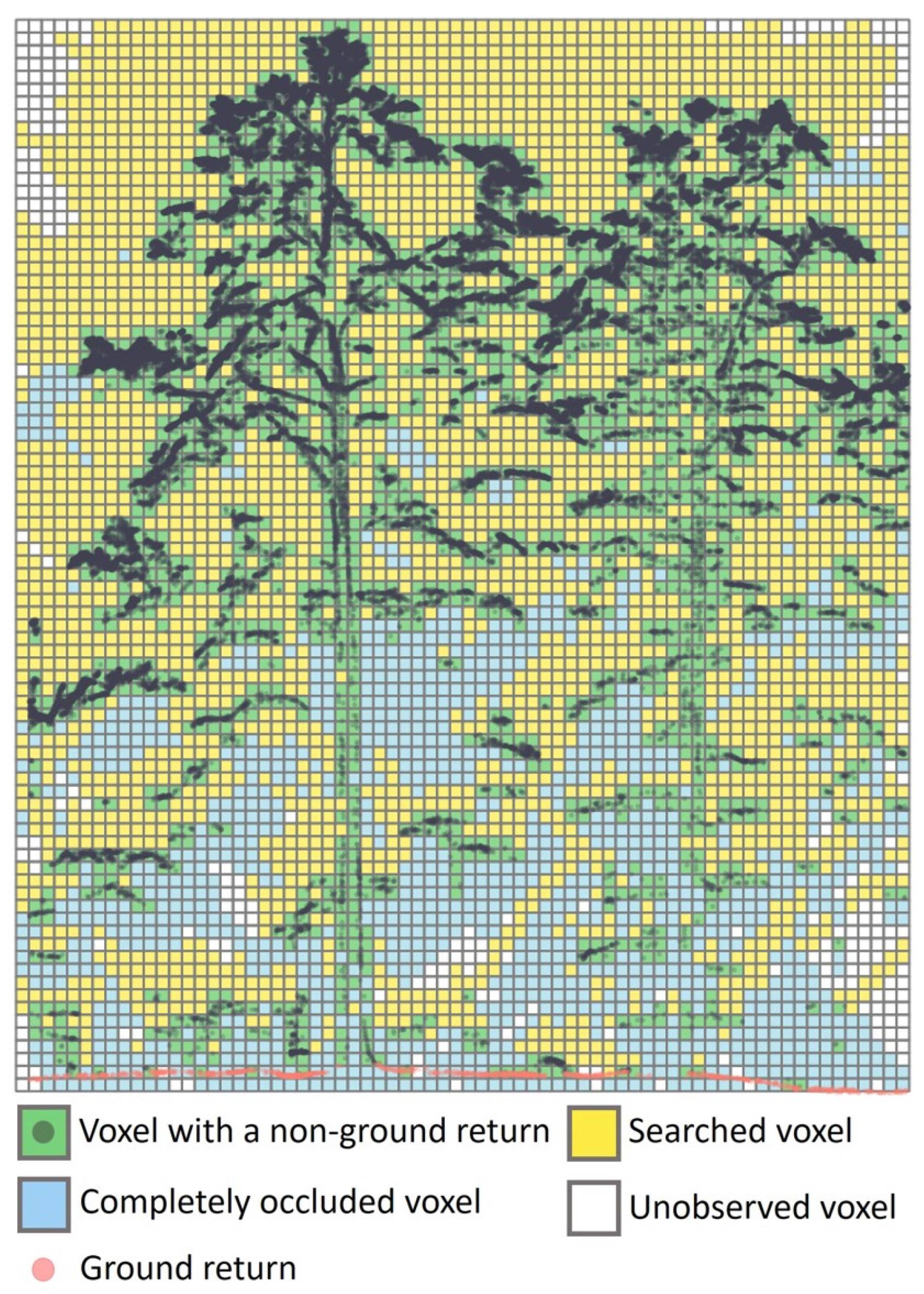
<p>High-resolution forest structure from a high-density drone. Squares are 0.5 m voxels. Voxels were classified into four categories using non-ground returns from drone lidar: voxels with one or more returns (green), voxels that were searched by laser pulses and contained no return (yellow), voxels with only occluded pulses (blue), and voxels with no returns, laser pulses, or occluded pulses (white). Grey dots on green voxels represent lidar returns. Darker grey dots indicate more returns in the voxel.</p> "> Figure 3
<p>Voxel traversal and voxel type determination. (<b>A</b>) Illustration of voxel traversal in a 2-D view featuring nine voxels and a laser pulse generating a return. All the squares represent occupied voxels. The solid yellow line segment represents a pulse trajectory. The green dot represents a lidar return. The black dot is the starting point of the pulse trajectory. Letters a–i are labels for the voxels. (<b>B</b>) Relationships among the voxels depicted in (<b>A</b>).</p> "> Figure 4
<p>Sampling completeness (the proportion of occupied voxels that were detected) as a function of pulse density and scan-angle range (plot 1). (<b>A</b>) When scan-angle range was decoupled from pulse density, sampling completeness was more strongly associated with pulse density than with scan-angle range. (<b>B</b>) Sampling completeness when scan-angle range was not decoupled from pulse density. Missing data points in (<b>A</b>) are associated with small sample sizes at certain combinations of scan-angle range and pulse density.</p> "> Figure 5
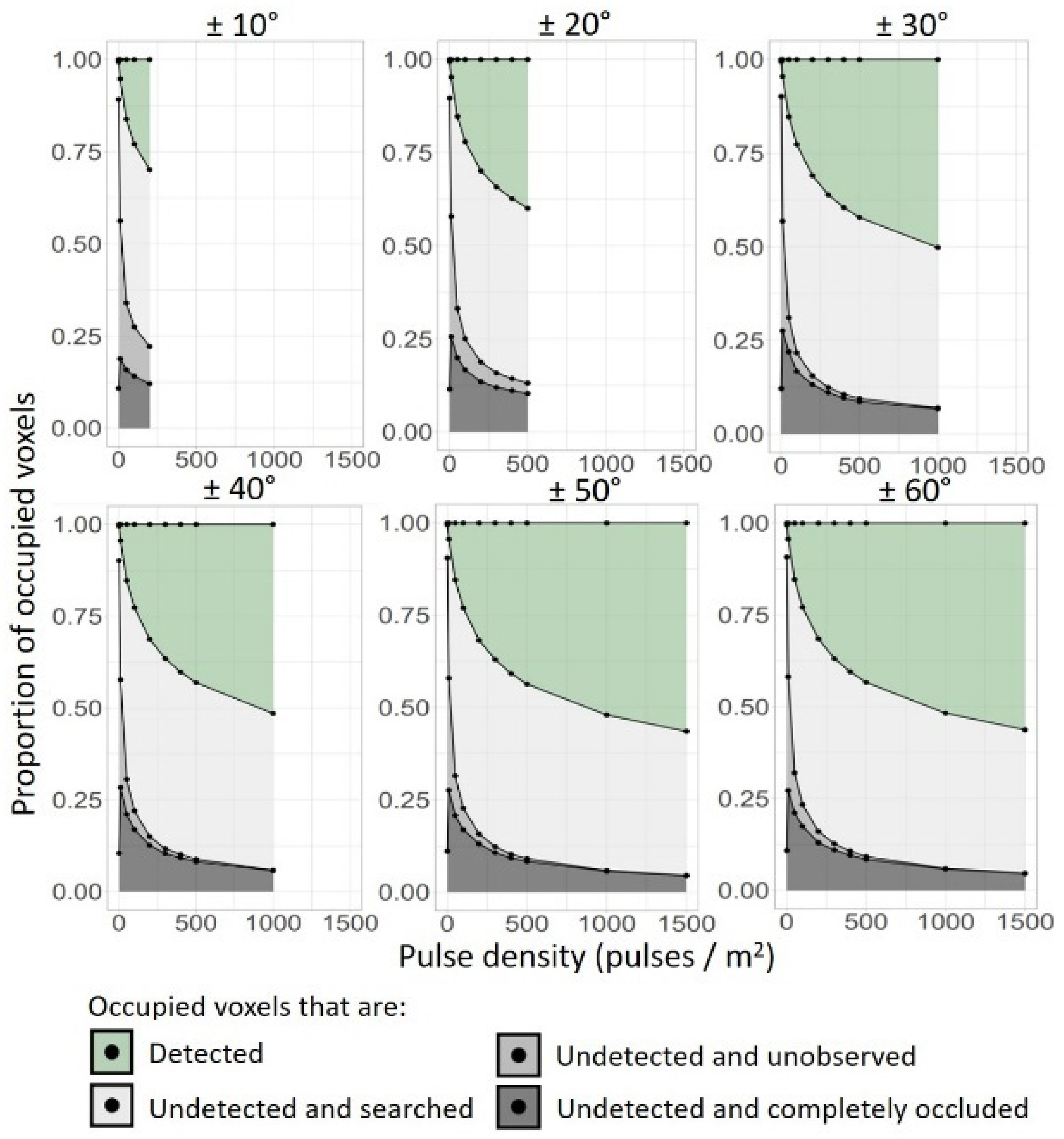
<p>Proportions of occupied voxels that were detected and undetected as a function of pulse density and scan-angle range (plot 1). On each of the six panels, from left to right, the black dots represent pulse densities of 1, 10, 50, 100, 200, 300, 400, 500, 1000, 1500 pulses/m<sup>2</sup>. Only 6 levels of scan-angle range (±10°, ±20°, ±30°, ±40°, ±50° and ±60°) are shown here because <a href="#remotesensing-16-02774-f004" class="html-fig">Figure 4</a> shows the limited impact of scan-angle range after decoupling its impact from pulse density. Missing data points are associated with small sample sizes at certain combinations of scan-angle range and pulse density.</p> "> Figure 6
<p>Proportions of different types of undetected voxels under different pulse densities and scan-angle ranges (plot 1). (<b>A</b>) Undetected and unsearched voxels. (<b>B</b>) Undetected and searched voxels. (<b>C</b>) Undetected and unobserved voxels. (<b>D</b>) Undetected and completely occluded voxels. Missing data points in each panel are associated with small sample sizes at some combinations of scan-angle range and pulse density. The number of undetected and unsearched voxels (<b>A</b>) is equal to the number of undetected and unobserved voxels (<b>C</b>) plus the number of undetected and completely occluded voxels (<b>D</b>).</p> "> Figure 7
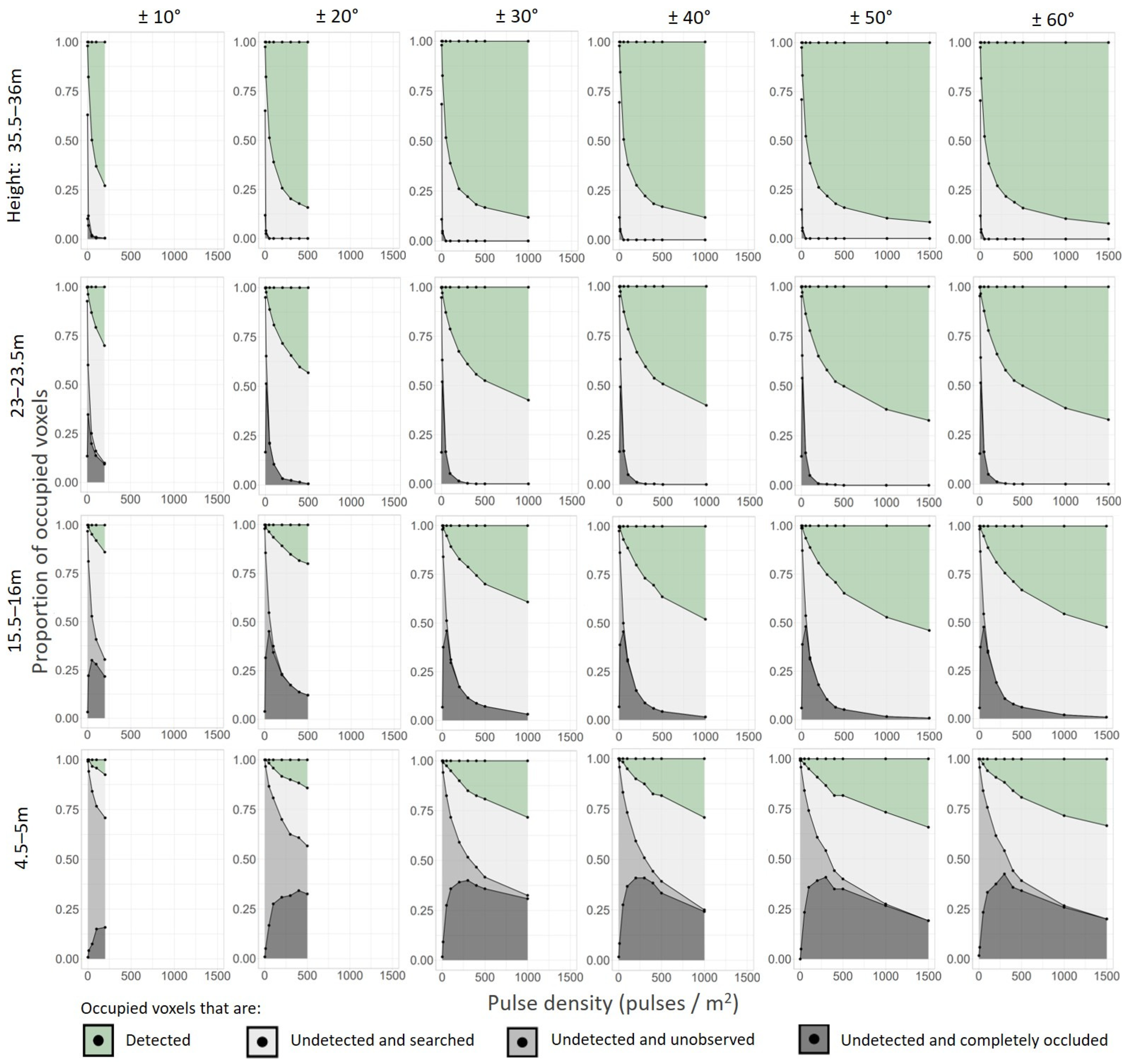
<p>Proportions of occupied voxels that were detected or undetected as a function of pulse density and scan-angle range at multiple heights above ground (Plot 1). Only 6 levels of scan-angle range (±10°, ±20°, ±30°, ±40°, ±50° and ±60°) are shown here because <a href="#remotesensing-16-02774-f004" class="html-fig">Figure 4</a> shows the limited impact of scan-angle range after decoupling its impact from pulse density. Missing data points are associated with small sample sizes at certain combinations of scan-angle range and pulse density. The number of occupied voxels at each height (i.e., the denominator for calculating proportions of different undetected voxels at each height) is shown in <a href="#remotesensing-16-02774-f0A15" class="html-fig">Figure A15</a>.</p> "> Figure 8
<p>Proportions of occupied voxels that were detected and undetected as a function of pulse density and scan-angle range at multiple heights above ground (plot 1). Only 6 levels of scan-angle range (±10°, ±20°, ±30°, ±40°, ±50° and ±60°) are shown here because <a href="#remotesensing-16-02774-f004" class="html-fig">Figure 4</a> shows the limited impact of scan-angle range after decoupling its impact from pulse density. Missing data points are associated with small sample sizes at certain combinations of scan-angle range and pulse density. The number of occupied voxels at each height (i.e., the denominator for calculating proportions of different undetected voxels at each height) is shown in <a href="#remotesensing-16-02774-f0A15" class="html-fig">Figure A15</a>.</p> "> Figure 9
<p>The proportion of undetected and searched voxels at different heights as a function of pulse density and scan-angle range in the 100 m<sup>2</sup> plot (Plot 1). Only 6 levels of scan-angle range (±10°, ±20°, ±30°, ±40°, ±50° and ±60°) are shown here because <a href="#remotesensing-16-02774-f004" class="html-fig">Figure 4</a> shows the limited impact of scan-angle range after decoupling its impact from pulse density. Missing data points are associated with small sample sizes at certain combinations of scan-angle range and pulse density.</p> "> Figure 10
<p>The proportion of undetected and completely occluded voxels at different heights as a function of pulse density and scan-angle range in the 100 m<sup>2</sup> plot (Plot 1). Only 6 levels of scan-angle range (±10°, ±20°, ±30°, ±40°, ±50° and ±60°) are shown here because <a href="#remotesensing-16-02774-f004" class="html-fig">Figure 4</a> shows the limited impact of scan-angle range after decoupling its impact from pulse density. Missing data points are associated with small sample sizes at some combinations of scan-angle range and pulse density.</p> "> Figure A1
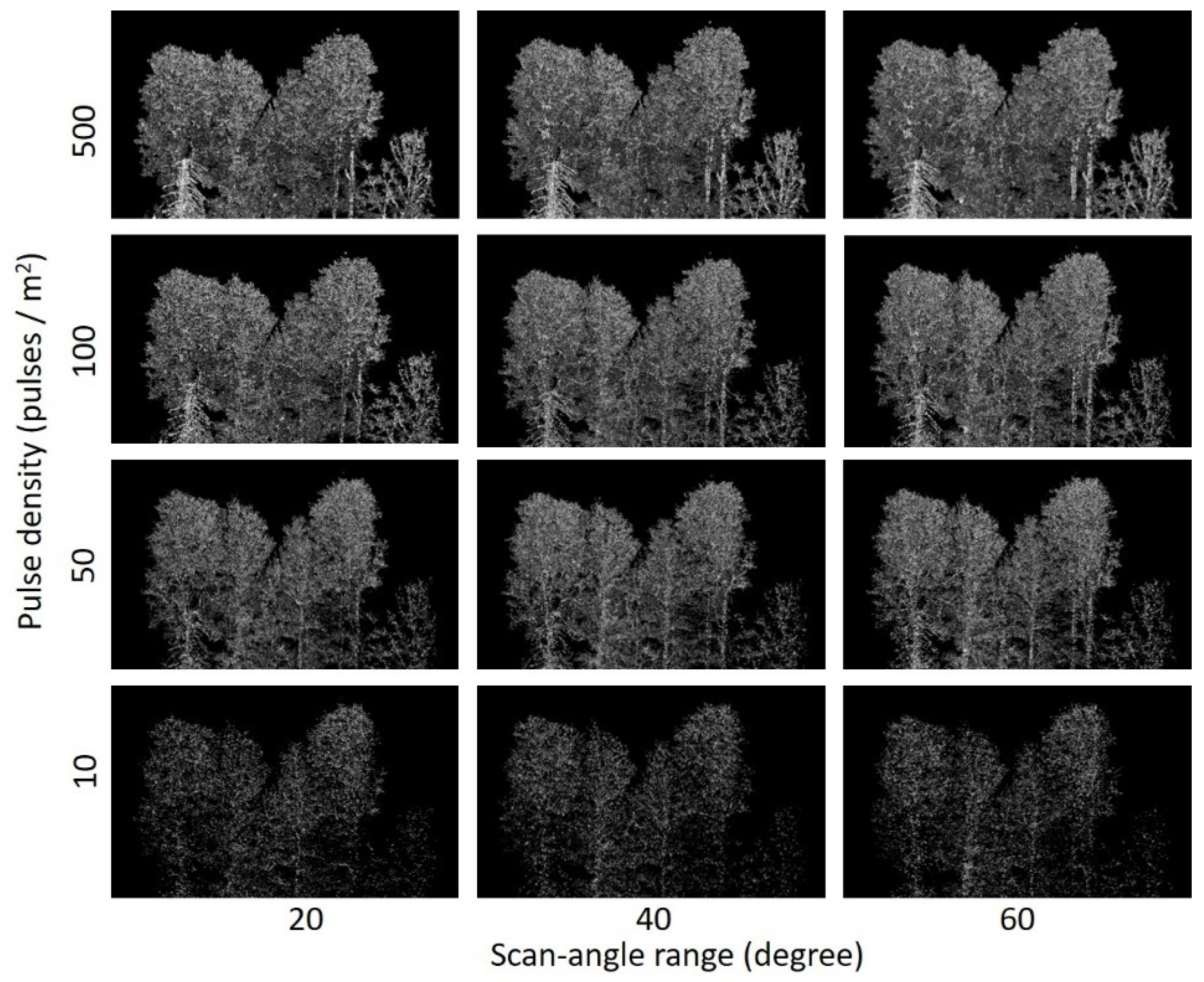
<p>Stem and branch structure as a function of pulse density and scan-angle range. The area is approximately 30 by 30 m in a temperate mountain forest in the southwest Czech Republic. The number of returns was more sensitive to pulse density than to scan-angle range.</p> "> Figure A2
<p>Stem and branch structure as a function of pulse density and scan-angle range, highlighting vegetation structure among prominent stems. Data are from high-density drone lidar in a temperate mountain forest in the southwest Czech Republic. The number of returns was more sensitive to pulse density than to scan-angle range.</p> "> Figure A3
<p>Stem and branch structure as a function of pulse density and scan-angle range, highlighting upper-canopy vegetation. Data are from high-density drone lidar in a temperate mountain forest in the southwest Czech Republic. The number of returns was more sensitive to pulse density than to scan-angle range.</p> "> Figure A4
<p>Proportions of occupied voxels that were detected and undetected as a function of pulse density and scan-angle range at Plot 2. On each of the six panels, from left to right, the black dots represent pulse densities of 1, 10, 50, 100, 200, 300, 400, 500, 1000, 1500 pulses/m<sup>2</sup>. Only 6 levels of scan-angle range (±10°, ±20°, ±30°, ±40°, ±50°, and ±60°) are shown here because <a href="#remotesensing-16-02774-f004" class="html-fig">Figure 4</a> shows the limited impact of scan-angle range after decoupling its impact from pulse density. Missing data points are associated with small sample sizes at certain combinations of scan-angle range and pulse density.</p> "> Figure A5
<p>Proportions of occupied voxels that were detected and undetected as a function of pulse density and scan-angle range at Plot 3. On each of the six panels, from left to right, the black dots represent pulse densities of 1, 10, 50, 100, 200, 300, 400, 500, 1000, 1500 pulses/m<sup>2</sup>. Only 6 levels of scan-angle range (±10°, ±20°, ±30°, ±40°, ±50°, and ±60°) are shown here because <a href="#remotesensing-16-02774-f004" class="html-fig">Figure 4</a> shows the limited impact of scan-angle range after decoupling its impact from pulse density. Missing data points are associated with small sample sizes at certain combinations of scan-angle range and pulse density.</p> "> Figure A6
<p>Proportions of occupied voxels that were detected and undetected as a function of pulse density and scan-angle range at Plot 4. On each of the six panels, from left to right, the black dots represent pulse densities of 1, 10, 50, 100, 200, 300, 400, 500, 1000, 1500 pulses/m<sup>2</sup>. Only 6 levels of scan-angle range (±10°, ±20°, ±30°, ±40°, ±50°, and ±60°) are shown here because <a href="#remotesensing-16-02774-f004" class="html-fig">Figure 4</a> shows the limited impact of scan-angle range after decoupling its impact from pulse density. Missing data points are associated with small sample sizes at certain combinations of scan-angle range and pulse density.</p> "> Figure A7
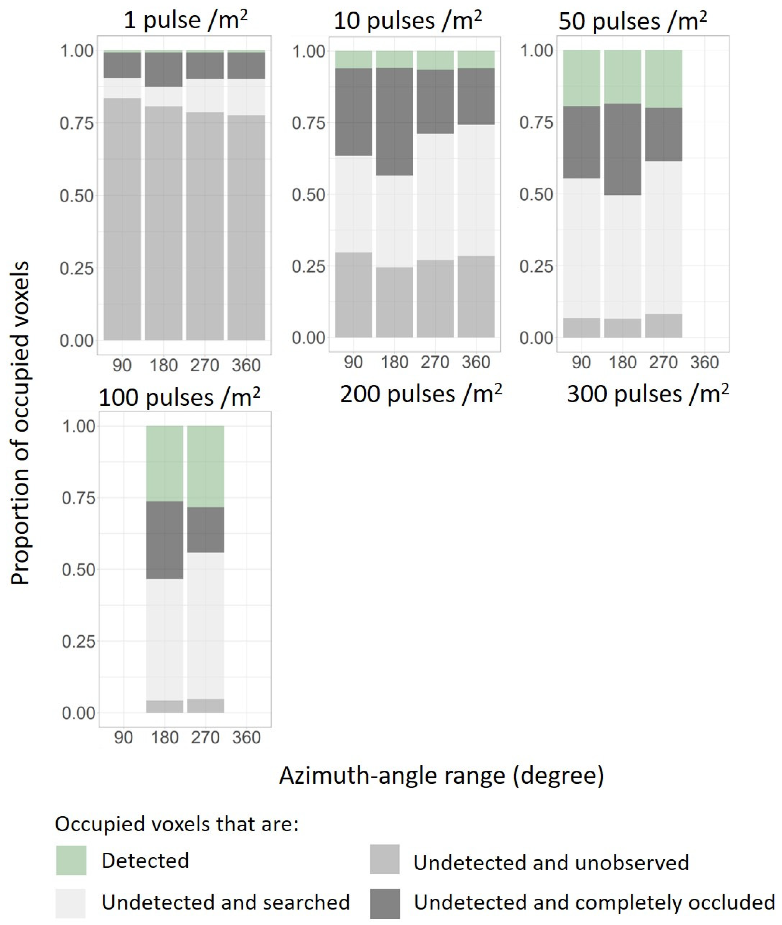
<p>Proportions of occupied voxels that were detected and undetected as a function of pulse density and azimuth-angle range (Plot 1). The azimuth-angle ranges were 0°–90°, 90°–180°, 180°–270°, and 270°–360°; they are labeled on the X-axis by the right bound (i.e., 90, 180, 270, 360, respectively). Missing data points are associated with small sample sizes at certain combinations of azimuth-angle range and pulse density.</p> "> Figure A8
<p>Proportions of occupied voxels that were detected and undetected as a function of pulse density and azimuth-angle range (Plot 2). The azimuth-angle ranges were 0°–90°, 90°–180°, 180°–270°, and 270°–360°; they are labeled on the X-axis by the right bound (i.e., 90, 180, 270, 360, respectively). Missing data points are associated with small sample sizes at certain combinations of azimuth-angle range and pulse density.</p> "> Figure A9
<p>Proportions of occupied voxels that were detected and undetected as a function of pulse density and azimuth-angle range (Plot 3). The azimuth-angle ranges were 0°–90°, 90°–180°, 180°–270°, and 270°–360°; they are labeled on the X-axis by the right bound (i.e., 90, 180, 270, 360, respectively). Missing data points are associated with small sample sizes at certain combinations of azimuth-angle range and pulse density.</p> "> Figure A10
<p>Proportions of occupied voxels that were detected and undetected as a function of pulse density and azimuth-angle range (Plot 4). The azimuth-angle ranges were 0°–90°, 90°–180°, 180°–270°, and 270°–360°; they are labeled on the X-axis by the right bound (i.e., 90, 180, 270, 360, respectively). Missing data points are associated with small sample sizes at certain combinations of azimuth-angle range and pulse density.</p> "> Figure A11
<p>Proportions of occupied voxels that were detected and undetected as a function of pulse density and scan-angle range at multiple heights above ground in a 100 m<sup>2</sup> plot (Plot 2). Missing data points are associated with small sample sizes at certain combinations of scan-angle range and pulse density.</p> "> Figure A12
<p>Proportions of occupied voxels that were detected and undetected as a function of pulse density and scan-angle range at multiple heights above ground in a 100 m<sup>2</sup> plot (Plot 3). Missing data points are associated with small sample sizes at certain combinations of scan-angle range and pulse density.</p> "> Figure A13
<p>Proportions of occupied voxels that were detected and undetected as a function of pulse density and scan-angle range at multiple heights aboveground in a 100 m<sup>2</sup> plot (Plot 4). Missing data points are associated with small sample sizes at certain combinations of scan-angle range and pulse density.</p> "> Figure A14
<p>The proportion of detected voxels at different heights as a function of pulse density and scan-angle range in the 1 ha plot. Only 6 levels of scan-angle range (±10°, ±20°, ±30°, ±40°, ±50° and ±60°) are shown here because <a href="#remotesensing-16-02774-f004" class="html-fig">Figure 4</a> shows the limited impact of scan-angle range after decoupling from pulse density. Missing data points are associated with small sample sizes at some combinations of scan-angle range and pulse density.</p> "> Figure A15
<p>The number of occupied voxels at each height above ground in a 100 m<sup>2</sup> plot (Plot 1).</p> "> Figure A16
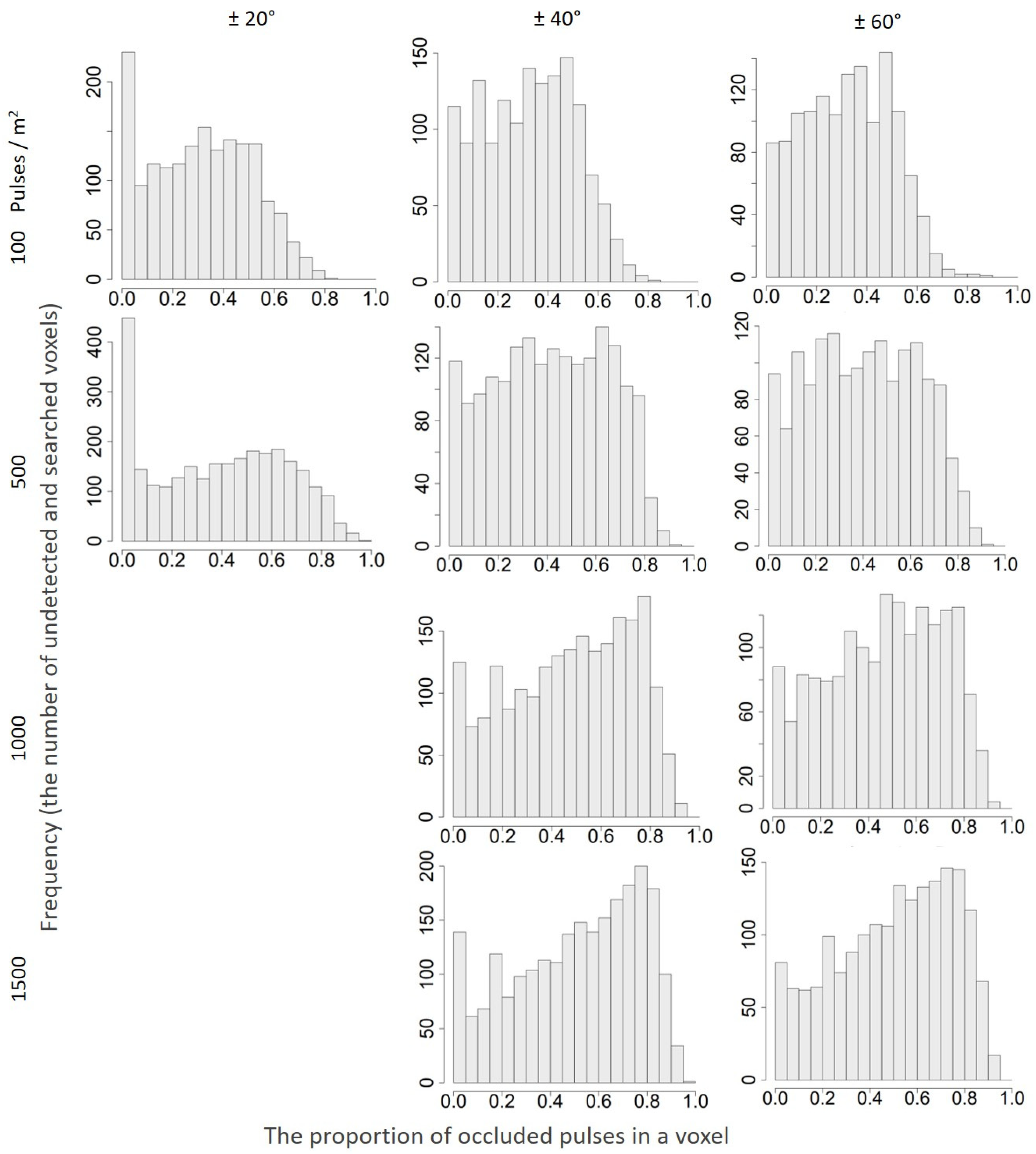
<p>Proportions of occluded pulses in undetected and searched voxels as a function of pulse density and scan-angle range (Plot 1). Missing panels are associated with small sample sizes at certain combinations of scan-angle range and pulse density.</p> ">
Abstract
:1. Introduction
2. Materials and Methods
2.1. Drone Lidar
2.2. Terrestrial Laser Scanning
2.3. Ray Tracing and Voxel-Traversal
2.3.1. Reconstruction of Pulse Trajectories
2.3.2. Voxel Traversal
2.4. Quantifying Sampling Completeness under Simulated Conditions
3. Results
3.1. Sampling Completeness under Different Pulse Densities and Scan-Angle Ranges
3.2. Undetected Voxels under Different Pulse Densities and Scan-Angle Ranges
3.3. Vertical Variability of Proportions of Different Types of Voxels
4. Discussion
4.1. Sampling Completeness under Different Pulse Densities and Scan-Angle Ranges
4.2. Undetected Voxels under Different Pulse Densities and Scan-Angle Ranges
4.3. Vertical Variability of Proportions of Different Types of Voxels
4.4. Future Work
5. Conclusions
Author Contributions
Funding
Data Availability Statement
Acknowledgments
Conflicts of Interest
Appendix A


| Model | R2 |
| 0.652 | |
| 0.650 | |
| 0.061 |
References
- Beer, C.; Reichstein, M.; Tomelleri, E.; Ciais, P.; Jung, M.; Carvalhais, N.; Rödenbeck, C.; Arain, M.A.; Baldocchi, D.; Bonan, G.B.; et al. Terrestrial Gross Carbon Dioxide Uptake: Global Distribution and Covariation with Climate. Science 2010, 329, 834–838. [Google Scholar] [CrossRef] [PubMed]
- Pan, Y.; Birdsey, R.A.; Phillips, O.L.; Jackson, R.B. The Structure, Distribution, and Biomass of the World’s Forests. Annu. Rev. Ecol. Evol. Syst. 2013, 44, 593–622. [Google Scholar] [CrossRef]
- FAO and UNEP. The State of the World’s Forests 2020: Forests, Biodiversity and People; The State of the World’s Forests (SOFO); FAO and UNEP: Rome, Italy, 2020; ISBN 978-92-5-132419-6. [Google Scholar]
- Morsdorf, F.; Kötz, B.; Meier, E.; Itten, K.I.; Allgöwer, B. Estimation of LAI and Fractional Cover from Small Footprint Airborne Laser Scanning Data Based on Gap Fraction. Remote Sens. Environ. 2006, 104, 50–61. [Google Scholar] [CrossRef]
- Yang, X.; Strahler, A.H.; Schaaf, C.B.; Jupp, D.L.B.; Yao, T.; Zhao, F.; Wang, Z.; Culvenor, D.S.; Newnham, G.J.; Lovell, J.L.; et al. Three-Dimensional Forest Reconstruction and Structural Parameter Retrievals Using a Terrestrial Full-Waveform Lidar Instrument (Echidna®). Remote Sens. Environ. 2013, 135, 36–51. [Google Scholar] [CrossRef]
- Pueschel, P.; Newnham, G.; Rock, G.; Udelhoven, T.; Werner, W.; Hill, J. The Influence of Scan Mode and Circle Fitting on Tree Stem Detection, Stem Diameter and Volume Extraction from Terrestrial Laser Scans. ISPRS J. Photogramm. Remote Sens. 2013, 77, 44–56. [Google Scholar] [CrossRef]
- Olsoy, P.J.; Glenn, N.F.; Clark, P.E.; Derryberry, D.R. Aboveground Total and Green Biomass of Dryland Shrub Derived from Terrestrial Laser Scanning. ISPRS J. Photogramm. Remote Sens. 2014, 88, 166–173. [Google Scholar] [CrossRef]
- Li, Y.; Guo, Q.; Su, Y.; Tao, S.; Zhao, K.; Xu, G. Retrieving the Gap Fraction, Element Clumping Index, and Leaf Area Index of Individual Trees Using Single-Scan Data from a Terrestrial Laser Scanner. ISPRS J. Photogramm. Remote Sens. 2017, 130, 308–316. [Google Scholar] [CrossRef]
- Roşca, S.; Suomalainen, J.; Bartholomeus, H.; Herold, M. Comparing Terrestrial Laser Scanning and Unmanned Aerial Vehicle Structure from Motion to Assess Top of Canopy Structure in Tropical Forests. Interface Focus 2018, 8, 20170038. [Google Scholar] [CrossRef] [PubMed]
- Liu, J.; Skidmore, A.K.; Wang, T.; Zhu, X.; Premier, J.; Heurich, M.; Beudert, B.; Jones, S. Variation of Leaf Angle Distribution Quantified by Terrestrial LiDAR in Natural European Beech Forest. ISPRS J. Photogramm. Remote Sens. 2019, 148, 208–220. [Google Scholar] [CrossRef]
- Disney, M.; Burt, A.; Wilkes, P.; Armston, J.; Duncanson, L. New 3D Measurements of Large Redwood Trees for Biomass and Structure. Sci. Rep. 2020, 10, 16721. [Google Scholar] [CrossRef]
- Coops, N.C.; Tompalski, P.; Goodbody, T.R.H.; Queinnec, M.; Luther, J.E.; Bolton, D.K.; White, J.C.; Wulder, M.A.; van Lier, O.R.; Hermosilla, T. Modelling Lidar-Derived Estimates of Forest Attributes over Space and Time: A Review of Approaches and Future Trends. Remote Sens. Environ. 2021, 260, 112477. [Google Scholar] [CrossRef]
- Saatchi, S.S.; Harris, N.L.; Brown, S.; Lefsky, M.; Mitchard, E.T.A.; Salas, W.; Zutta, B.R.; Buermann, W.; Lewis, S.L.; Hagen, S.; et al. Benchmark Map of Forest Carbon Stocks in Tropical Regions across Three Continents. Proc. Natl. Acad. Sci. USA 2011, 108, 9899–9904. [Google Scholar] [CrossRef] [PubMed]
- Stovall, A.E.L.; Shugart, H.H. Improved Biomass Calibration and Validation with Terrestrial LiDAR: Implications for Future LiDAR and SAR Missions. IEEE J. Sel. Top. Appl. Earth Obs. Remote Sens. 2018, 11, 3527–3537. [Google Scholar] [CrossRef]
- Disney, M.; Burt, A.; Calders, K.; Schaaf, C.; Stovall, A. Innovations in Ground and Airborne Technologies as Reference and for Training and Validation: Terrestrial Laser Scanning (TLS). Surv. Geophys. 2019, 40, 937–958. [Google Scholar] [CrossRef]
- Duncanson, L.; Armston, J.; Disney, M.; Avitabile, V.; Barbier, N.; Calders, K.; Carter, S.; Chave, J.; Herold, M.; Crowther, T.W.; et al. The Importance of Consistent Global Forest Aboveground Biomass Product Validation. Surv. Geophys. 2019, 40, 979–999. [Google Scholar] [CrossRef]
- Duncanson, L.; Armston, J.; Disney, M.; Avitabile, V.; Barbier, N.; Calders, K.; Carter, S.; Chave, J.; Herold, M.; MacBean, N.; et al. Aboveground Woody Biomass Product Validation Good Practices Protocol. Version 1.0. In Good Practices for Satellite Derived Land Product Validation; Duncanson, L., Disney, M., Armston, J., Nickeson, J., Minor, D., Camacho, F., Eds.; Land Product Validation Subgroup (WGCV/CEOS), 2021; p. 236. Available online: https://doi.org/10.5067/doc/ceoswgcv/lpv/agb.001 (accessed on 10 July 2024).
- Beland, M.; Parker, G.; Sparrow, B.; Harding, D.; Chasmer, L.; Phinn, S.; Antonarakis, A.; Strahler, A. On Promoting the Use of Lidar Systems in Forest Ecosystem Research. For. Ecol. Manag. 2019, 450, 117484. [Google Scholar] [CrossRef]
- Smith, M.N.; Stark, S.C.; Taylor, T.C.; Ferreira, M.L.; de Oliveira, E.; Restrepo-Coupe, N.; Chen, S.; Woodcock, T.; dos Santos, D.B.; Alves, L.F.; et al. Seasonal and Drought-Related Changes in Leaf Area Profiles Depend on Height and Light Environment in an Amazon Forest. New Phytol. 2019, 222, 1284–1297. [Google Scholar] [CrossRef]
- Ma, L.; Hurtt, G.; Tang, H.; Lamb, R.; Lister, A.; Chini, L.; Dubayah, R.; Armston, J.; Campbell, E.; Duncanson, L.; et al. Spatial Heterogeneity of Global Forest Aboveground Carbon Stocks and Fluxes Constrained by Spaceborne Lidar Data and Mechanistic Modeling. Glob. Chang. Biol. 2023, 29, 3378–3394. [Google Scholar] [CrossRef]
- Liang, X.; Kankare, V.; Hyyppä, J.; Wang, Y.; Kukko, A.; Haggrén, H.; Yu, X.; Kaartinen, H.; Jaakkola, A.; Guan, F.; et al. Terrestrial Laser Scanning in Forest Inventories. ISPRS J. Photogramm. Remote Sens. 2016, 115, 63–77. [Google Scholar] [CrossRef]
- Calders, K.; Adams, J.; Armston, J.; Bartholomeus, H.; Bauwens, S.; Bentley, L.P.; Chave, J.; Danson, F.M.; Demol, M.; Disney, M.; et al. Terrestrial Laser Scanning in Forest Ecology: Expanding the Horizon. Remote Sens. Environ. 2020, 251, 112102. [Google Scholar] [CrossRef]
- Hopkinson, C.; Chasmer, L.; Young-Pow, C.; Treitz, P. Assessing Forest Metrics with a Ground-Based Scanning Lidar. Can. J. For. Res. 2004, 34, 573–583. [Google Scholar] [CrossRef]
- Strahler, A.H.; Jupp, D.L.B.; Woodcock, C.E.; Schaaf, C.B.; Yao, T.; Zhao, F.; Yang, X.; Lovell, J.; Culvenor, D.; Newnham, G.; et al. Retrieval of Forest Structural Parameters Using a Ground-Based Lidar Instrument (Echidna®). Can. J. Remote Sens. 2008, 34, S426–S440. [Google Scholar] [CrossRef]
- Dassot, M.; Colin, A.; Santenoise, P.; Fournier, M.; Constant, T. Terrestrial Laser Scanning for Measuring the Solid Wood Volume, Including Branches, of Adult Standing Trees in the Forest Environment. Comput. Electron. Agric. 2012, 89, 86–93. [Google Scholar] [CrossRef]
- Zheng, G.; Moskal, L.M.; Kim, S.-H. Retrieval of Effective Leaf Area Index in Heterogeneous Forests with Terrestrial Laser Scanning. IEEE Trans. Geosci. Remote Sens. 2013, 51, 777–786. [Google Scholar] [CrossRef]
- Calders, K.; Newnham, G.; Burt, A.; Murphy, S.; Raumonen, P.; Herold, M.; Culvenor, D.; Avitabile, V.; Disney, M.; Armston, J.; et al. Nondestructive Estimates of Above-Ground Biomass Using Terrestrial Laser Scanning. Methods Ecol. Evol. 2015, 6, 198–208. [Google Scholar] [CrossRef]
- Wang, Q.; Pang, Y.; Chen, D.; Liang, X.; Lu, J. Lidar Biomass Index: A Novel Solution for Tree-Level Biomass Estimation Using 3D Crown Information. For. Ecol. Manag. 2021, 499, 119542. [Google Scholar] [CrossRef]
- Bornand, A.; Rehush, N.; Morsdorf, F.; Thürig, E.; Abegg, M. Individual Tree Volume Estimation with Terrestrial Laser Scanning: Evaluating Reconstructive and Allometric Approaches. Agric. For. Meteorol. 2023, 341, 109654. [Google Scholar] [CrossRef]
- Brede, B.; Lau, A.; Bartholomeus, H.M.; Kooistra, L. Comparing RIEGL RiCOPTER UAV LiDAR Derived Canopy Height and DBH with Terrestrial LiDAR. Sensors 2017, 17, 2371. [Google Scholar] [CrossRef]
- Wilkes, P.; Lau, A.; Disney, M.; Calders, K.; Burt, A.; de Tanago, J.G.; Bartholomeus, H.; Brede, B.; Herold, M. Data Acquisition Considerations for Terrestrial Laser Scanning of Forest Plots. Remote Sens. Environ. 2017, 196, 140–153. [Google Scholar] [CrossRef]
- Calders, K.; Armston, J.; Newnham, G.; Herold, M.; Goodwin, N. Implications of Sensor Configuration and Topography on Vertical Plant Profiles Derived from Terrestrial LiDAR. Agric. For. Meteorol. 2014, 194, 104–117. [Google Scholar] [CrossRef]
- Chasmer, L.; Hopkinson, C.; Treitz, P. Assessing the Three-Dimensional Frequency Distribution of Airborne and Ground-Based Lidar Data for Red Pine and Mixed Deciduous Forest Plots. Int. Arch. Photogramm. Remote Sens. Spat. Inf. Sci. 2004, 36, W2. [Google Scholar]
- LaRue, E.A.; Wagner, F.W.; Fei, S.; Atkins, J.W.; Fahey, R.T.; Gough, C.M.; Hardiman, B.S. Compatibility of Aerial and Terrestrial LiDAR for Quantifying Forest Structural Diversity. Remote Sens. 2020, 12, 1407. [Google Scholar] [CrossRef]
- Zhao, K.; Popescu, S.; Nelson, R. Lidar Remote Sensing of Forest Biomass: A Scale-Invariant Estimation Approach Using Airborne Lasers. Remote Sens. Environ. 2009, 113, 182–196. [Google Scholar] [CrossRef]
- Xu, L.; Saatchi, S.S.; Shapiro, A.; Meyer, V.; Ferraz, A.; Yang, Y.; Bastin, J.-F.; Banks, N.; Boeckx, P.; Verbeeck, H.; et al. Spatial Distribution of Carbon Stored in Forests of the Democratic Republic of Congo. Sci. Rep. 2017, 7, 15030. [Google Scholar] [CrossRef] [PubMed]
- Saarela, S.; Wästlund, A.; Holmström, E.; Mensah, A.A.; Holm, S.; Nilsson, M.; Fridman, J.; Ståhl, G. Mapping Aboveground Biomass and Its Prediction Uncertainty Using LiDAR and Field Data, Accounting for Tree-Level Allometric and LiDAR Model Errors. For. Ecosyst. 2020, 7, 43. [Google Scholar] [CrossRef]
- Ryding, J.; Williams, E.; Smith, M.J.; Eichhorn, M.P. Assessing Handheld Mobile Laser Scanners for Forest Surveys. Remote Sens. 2015, 7, 1095–1111. [Google Scholar] [CrossRef]
- Bauwens, S.; Bartholomeus, H.; Calders, K.; Lejeune, P. Forest Inventory with Terrestrial LiDAR: A Comparison of Static and Hand-Held Mobile Laser Scanning. Forests 2016, 7, 127. [Google Scholar] [CrossRef]
- Hyyppä, E.; Kukko, A.; Kaijaluoto, R.; White, J.C.; Wulder, M.A.; Pyörälä, J.; Liang, X.; Yu, X.; Wang, Y.; Kaartinen, H.; et al. Accurate Derivation of Stem Curve and Volume Using Backpack Mobile Laser Scanning. ISPRS J. Photogramm. Remote Sens. 2020, 161, 246–262. [Google Scholar] [CrossRef]
- Liang, X.; Kukko, A.; Kaartinen, H.; Hyyppä, J.; Yu, X.; Jaakkola, A.; Wang, Y. Possibilities of a Personal Laser Scanning System for Forest Mapping and Ecosystem Services. Sensors 2014, 14, 1228–1248. [Google Scholar] [CrossRef]
- Liang, X.; Hyyppä, J.; Kukko, A.; Kaartinen, H.; Jaakkola, A.; Yu, X. The Use of a Mobile Laser Scanning System for Mapping Large Forest Plots. IEEE Geosci. Remote Sens. Lett. 2014, 11, 1504–1508. [Google Scholar] [CrossRef]
- Jaakkola, A.; Hyyppä, J.; Kukko, A.; Yu, X.; Kaartinen, H.; Lehtomäki, M.; Lin, Y. A Low-Cost Multi-Sensoral Mobile Mapping System and Its Feasibility for Tree Measurements. ISPRS J. Photogramm. Remote Sens. 2010, 65, 514–522. [Google Scholar] [CrossRef]
- Yang, B.; Fang, L.; Li, J. Semi-Automated Extraction and Delineation of 3D Roads of Street Scene from Mobile Laser Scanning Point Clouds. ISPRS J. Photogramm. Remote Sens. 2013, 79, 80–93. [Google Scholar] [CrossRef]
- Kellner, J.R.; Armston, J.; Birrer, M.; Cushman, K.C.; Duncanson, L.; Eck, C.; Falleger, C.; Imbach, B.; Král, K.; Krůček, M. New Opportunities for Forest Remote Sensing through Ultra-High-Density Drone Lidar. Surv. Geophys. 2019, 40, 959–977. [Google Scholar] [CrossRef]
- Resop, J.P.; Lehmann, L.; Hession, W.C. Drone Laser Scanning for Modeling Riverscape Topography and Vegetation: Comparison with Traditional Aerial Lidar. Drones 2019, 3, 35. [Google Scholar] [CrossRef]
- Puliti, S.; Dash, J.P.; Watt, M.S.; Breidenbach, J.; Pearse, G.D. A Comparison of UAV Laser Scanning, Photogrammetry and Airborne Laser Scanning for Precision Inventory of Small-Forest Properties. For. Int. J. For. Res. 2020, 93, 150–162. [Google Scholar] [CrossRef]
- Qi, Y.; Coops, N.C.; Daniels, L.D.; Butson, C.R. Comparing Tree Attributes Derived from Quantitative Structure Models Based on Drone and Mobile Laser Scanning Point Clouds across Varying Canopy Cover Conditions. ISPRS J. Photogramm. Remote Sens. 2022, 192, 49–65. [Google Scholar] [CrossRef]
- Brede, B.; Bartholomeus, H.M.; Barbier, N.; Pimont, F.; Vincent, G.; Herold, M. Peering through the Thicket: Effects of UAV LiDAR Scanner Settings and Flight Planning on Canopy Volume Discovery. Int. J. Appl. Earth Obs. Geoinf. 2022, 114, 103056. [Google Scholar] [CrossRef]
- Shui, W.; Li, H.; Zhang, Y.; Jiang, C.; Zhu, S.; Wang, Q.; Liu, Y.; Zong, S.; Huang, Y.; Ma, M. Is an Unmanned Aerial Vehicle (UAV) Suitable for Extracting the Stand Parameters of Inaccessible Underground Forests of Karst Tiankeng? Remote Sens. 2022, 14, 4128. [Google Scholar] [CrossRef]
- Barazzetti, L.; Previtali, M.; Cantini, L.; Oteri, A.M. Digital Recording of Historical Defensive Structures in Mountainous Areas Using Drones: Considerations and Comparisons. Drones 2023, 7, 512. [Google Scholar] [CrossRef]
- Kükenbrink, D.; Schneider, F.D.; Leiterer, R.; Schaepman, M.E.; Morsdorf, F. Quantification of Hidden Canopy Volume of Airborne Laser Scanning Data Using a Voxel Traversal Algorithm. Remote Sens. Environ. 2017, 194, 424–436. [Google Scholar] [CrossRef]
- Torralba, J.; Carbonell-Rivera, J.P.; Ruiz, L.Á.; Crespo-Peremarch, P. Analyzing TLS Scan Distribution and Point Density for the Estimation of Forest Stand Structural Parameters. Forests 2022, 13, 2115. [Google Scholar] [CrossRef]
- Hopkinson, C. The Influence of Lidar Acquisition Settings on Canopy Penetration and Laser Pulse Return Characteristics. In Proceedings of the 2006 IEEE International Symposium on Geoscience and Remote Sensing, Denver, CO, USA, 31 July–4 August 2006; pp. 2420–2423. [Google Scholar]
- Dayal, K.R.; Durrieu, S.; Lahssini, K.; Alleaume, S.; Bouvier, M.; Monnet, J.-M.; Renaud, J.-P.; Revers, F. An Investigation into Lidar Scan Angle Impacts on Stand Attribute Predictions in Different Forest Environments. ISPRS J. Photogramm. Remote Sens. 2022, 193, 314–338. [Google Scholar] [CrossRef]
- Musselman, K.N.; Margulis, S.A.; Molotch, N.P. Estimation of Solar Direct Beam Transmittance of Conifer Canopies from Airborne LiDAR. Remote Sens. Environ. 2013, 136, 402–415. [Google Scholar] [CrossRef]
- Cifuentes, R.; Van der Zande, D.; Farifteh, J.; Salas, C.; Coppin, P. Effects of Voxel Size and Sampling Setup on the Estimation of Forest Canopy Gap Fraction from Terrestrial Laser Scanning Data. Agric. For. Meteorol. 2014, 194, 230–240. [Google Scholar] [CrossRef]
- Magney, T.S.; Eitel, J.U.H.; Griffin, K.L.; Boelman, N.T.; Greaves, H.E.; Prager, C.M.; Logan, B.A.; Zheng, G.; Ma, L.; Fortin, E.A.; et al. LiDAR Canopy Radiation Model Reveals Patterns of Photosynthetic Partitioning in an Arctic Shrub. Agric. For. Meteorol. 2016, 221, 78–93. [Google Scholar] [CrossRef]
- Li, W.; Guo, Q.; Tao, S.; Su, Y. VBRT: A Novel Voxel-Based Radiative Transfer Model for Heterogeneous Three-Dimensional Forest Scenes. Remote Sens. Environ. 2018, 206, 318–335. [Google Scholar] [CrossRef]
- Xie, D.; Wang, X.; Qi, J.; Chen, Y.; Mu, X.; Zhang, W.; Yan, G. Reconstruction of Single Tree with Leaves Based on Terrestrial LiDAR Point Cloud Data. Remote Sens. 2018, 10, 686. [Google Scholar] [CrossRef]
- Disney, M.; Lewis, P.; Saich, P. 3D Modelling of Forest Canopy Structure for Remote Sensing Simulations in the Optical and Microwave Domains. Remote Sens. Environ. 2006, 100, 114–132. [Google Scholar] [CrossRef]
- Van der Zande, D.; Mereu, S.; Nadezhdina, N.; Cermak, J.; Muys, B.; Coppin, P.; Manes, F. 3D Upscaling of Transpiration from Leaf to Tree Using Ground-Based LiDAR: Application on a Mediterranean Holm Oak (Quercus ilex L.) Tree. Agric. For. Meteorol. 2009, 149, 1573–1583. [Google Scholar] [CrossRef]
- Bienert, A.; Queck, R.; Schmidt, A.; Bernhofer, C.; Maas, H.-G. Voxel Space Analysis of Terrestrial Laser Scans in Forests for Wind Field Modelling. Int. Arch. Photogramm. Remote Sens. Spat. Inf. Sci. 2010, 38, 92–97. [Google Scholar]
- Béland, M.; Widlowski, J.-L.; Fournier, R.A.; Côté, J.-F.; Verstraete, M.M. Estimating Leaf Area Distribution in Savanna Trees from Terrestrial LiDAR Measurements. Agric. For. Meteorol. 2011, 151, 1252–1266. [Google Scholar] [CrossRef]
- Béland, M.; Widlowski, J.-L.; Fournier, R.A. A Model for Deriving Voxel-Level Tree Leaf Area Density Estimates from Ground-Based LiDAR. Environ. Model. Softw. 2014, 51, 184–189. [Google Scholar] [CrossRef]
- Stovall, A.E.L.; Vorster, A.G.; Anderson, R.S.; Evangelista, P.H.; Shugart, H.H. Non-Destructive Aboveground Biomass Estimation of Coniferous Trees Using Terrestrial LiDAR. Remote Sens. Environ. 2017, 200, 31–42. [Google Scholar] [CrossRef]
- Paynter, I.; Genest, D.; Saenz, E.; Peri, F.; Li, Z.; Strahler, A.; Schaaf, C. Quality Assessment of Terrestrial Laser Scanner Ecosystem Observations Using Pulse Trajectories. IEEE Trans. Geosci. Remote Sens. 2018, 56, 6324–6333. [Google Scholar] [CrossRef]
- Zong, X.; Wang, T.; Skidmore, A.K.; Heurich, M. The Impact of Voxel Size, Forest Type, and Understory Cover on Visibility Estimation in Forests Using Terrestrial Laser Scanning. GIScience Remote Sens. 2021, 58, 323–339. [Google Scholar] [CrossRef]
- Morsdorf, F.; Frey, O.; Koetz, B.; Meier, E. Ray Tracing for Modeling of Small Footprint Airborne Laser Scanning Returns. Int. Arch. Photogramm. Remote Sens. Spat. Inf. Sci. 2007, 36, 249–299. [Google Scholar]
- Korpela, I.; Hovi, A.; Morsdorf, F. Understory Trees in Airborne LiDAR Data—Selective Mapping Due to Transmission Losses and Echo-Triggering Mechanisms. Remote Sens. Environ. 2012, 119, 92–104. [Google Scholar] [CrossRef]
- Vincent, G.; Antin, C.; Laurans, M.; Heurtebize, J.; Durrieu, S.; Lavalley, C.; Dauzat, J. Mapping Plant Area Index of Tropical Evergreen Forest by Airborne Laser Scanning. A Cross-Validation Study Using LAI2200 Optical Sensor. Remote Sens. Environ. 2017, 198, 254–266. [Google Scholar] [CrossRef]
- Gastellu-Etchegorry, J.-P.; Yin, T.; Lauret, N.; Grau, E.; Rubio, J.; Cook, B.D.; Morton, D.C.; Sun, G. Simulation of Satellite, Airborne and Terrestrial LiDAR with DART (I): Waveform Simulation with Quasi-Monte Carlo Ray Tracing. Remote Sens. Environ. 2016, 184, 418–435. [Google Scholar] [CrossRef]
- Yang, X.; Wang, Y.; Yin, T.; Wang, C.; Lauret, N.; Regaieg, O.; Xi, X.; Gastellu-Etchegorry, J.P. Comprehensive LiDAR Simulation with Efficient Physically-Based DART-Lux Model (I): Theory, Novelty, and Consistency Validation. Remote Sens. Environ. 2022, 272, 112952. [Google Scholar] [CrossRef]
- Winiwarter, L.; Esmorís Pena, A.M.; Weiser, H.; Anders, K.; Martínez Sánchez, J.; Searle, M.; Höfle, B. Virtual Laser Scanning with HELIOS++: A Novel Take on Ray Tracing-Based Simulation of Topographic Full-Waveform 3D Laser Scanning. Remote Sens. Environ. 2022, 269, 112772. [Google Scholar] [CrossRef]
- Amanatides, J.; Woo, A. A Fast Voxel Traversal Algorithm for Ray Tracing. Eurographics 1987, 87, 3–10. [Google Scholar]
- Schneider, F.D.; Kükenbrink, D.; Schaepman, M.E.; Schimel, D.S.; Morsdorf, F. Quantifying 3D Structure and Occlusion in Dense Tropical and Temperate Forests Using Close-Range LiDAR. Agric. For. Meteorol. 2019, 268, 249–257. [Google Scholar] [CrossRef]
- Anderson-Teixeira, K.J.; Davies, S.J.; Bennett, A.C.; Gonzalez-Akre, E.B.; Muller-Landau, H.C.; Wright, S.J.; Abu Salim, K.; Almeyda Zambrano, A.M.; Alonso, A.; Baltzer, J.L.; et al. CTFS-ForestGEO: A Worldwide Network Monitoring Forests in an Era of Global Change. Glob. Chang. Biol. 2015, 21, 528–549. [Google Scholar] [CrossRef]
- Janík, D.; Král, K.; Adam, D.; Hort, L.; Samonil, P.; Unar, P.; Vrska, T.; McMahon, S. Tree Spatial Patterns of Fagus Sylvatica Expansion over 37 years. For. Ecol. Manag. 2016, 375, 134–145. [Google Scholar] [CrossRef]
- Cushman, K.C.; Armston, J.; Dubayah, R.; Duncanson, L.; Hancock, S.; Janík, D.; Král, K.; Krůček, M.; Minor, D.M.; Tang, H.; et al. Impact of Leaf Phenology on Estimates of Aboveground Biomass Density in a Deciduous Broadleaf Forest from Simulated GEDI Lidar. Environ. Res. Lett. 2023, 18, 065009. [Google Scholar] [CrossRef]
- Zhang, K.; Chen, S.-C.; Whitman, D.; Shyu, M.-L.; Yan, J.; Zhang, C. A Progressive Morphological Filter for Removing Nonground Measurements from Airborne LIDAR Data. IEEE Trans. Geosci. Remote Sens. 2003, 41, 872–882. [Google Scholar] [CrossRef]
- Krůček, M.; Král, K.; Cushman, K.C.; Missarov, A.; Kellner, J.R. Supervised Segmentation of Ultra-High-Density Drone Lidar for Large-Area Mapping of Individual Trees. Remote Sens. 2020, 12, 3260. [Google Scholar] [CrossRef]
- Trochta, J.; Krůček, M.; Vrška, T.; Král, K. 3D Forest: An Application for Descriptions of Three-Dimensional Forest Structures Using Terrestrial LiDAR. PLoS ONE 2017, 12, e0176871. [Google Scholar] [CrossRef]
- Terryn, L.; Calders, K.; Bartholomeus, H.; Bartolo, R.E.; Brede, B.; D’hont, B.; Disney, M.; Herold, M.; Lau, A.; Shenkin, A.; et al. Quantifying Tropical Forest Structure through Terrestrial and UAV Laser Scanning Fusion in Australian Rainforests. Remote Sens. Environ. 2022, 271, 112912. [Google Scholar] [CrossRef]
- Lovell, J.L.; Jupp, D.L.B.; Newnham, G.J.; Culvenor, D.S. Measuring Tree Stem Diameters Using Intensity Profiles from Ground-Based Scanning Lidar from a Fixed Viewpoint. ISPRS J. Photogramm. Remote Sens. 2011, 66, 46–55. [Google Scholar] [CrossRef]
- Liang, X.; Litkey, P.; Hyyppa, J.; Kaartinen, H.; Vastaranta, M.; Holopainen, M. Automatic Stem Mapping Using Single-Scan Terrestrial Laser Scanning. IEEE Trans. Geosci. Remote Sens. 2012, 50, 661–670. [Google Scholar] [CrossRef]
- Murphy, G.E.; Acuna, M.A.; Dumbrell, I. Tree Value and Log Product Yield Determination in Radiata Pine (Pinus radiata) Plantations in Australia: Comparisons of Terrestrial Laser Scanning with a Forest Inventory System and Manual Measurements. Can. J. For. Res. 2010, 40, 2223–2233. [Google Scholar] [CrossRef]


| Plot | 1 ha | 100 m2 | |||
|---|---|---|---|---|---|
| 1 | 2 | 3 | 4 | ||
| Mean point density (points/m2) | 3354 | 3870 | 3881 | 3828 | 2953 |
| Stem density (stems/m2) | 0.3 | 0.2 | 0.5 | 0.03 | 0.2 |
| Mean DBH (cm) | 5.2 | 9.3 | 2.4 | 47.7 | 9.6 |
| Maximum DBH (cm) | 134.2 | 60.0 | 37.0 | 61.5 | 73.0 |
| Minimum DBH (cm) | 1.0 | 1.1 | 1.0 | 39.4 | 1.0 |
Disclaimer/Publisher’s Note: The statements, opinions and data contained in all publications are solely those of the individual author(s) and contributor(s) and not of MDPI and/or the editor(s). MDPI and/or the editor(s) disclaim responsibility for any injury to people or property resulting from any ideas, methods, instructions or products referred to in the content. |
© 2024 by the authors. Licensee MDPI, Basel, Switzerland. This article is an open access article distributed under the terms and conditions of the Creative Commons Attribution (CC BY) license (https://creativecommons.org/licenses/by/4.0/).
Share and Cite
Zhang, D.; Král, K.; Krůček, M.; Cushman, K.C.; Kellner, J.R. Near-Complete Sampling of Forest Structure from High-Density Drone Lidar Demonstrated by Ray Tracing. Remote Sens. 2024, 16, 2774. https://doi.org/10.3390/rs16152774
Zhang D, Král K, Krůček M, Cushman KC, Kellner JR. Near-Complete Sampling of Forest Structure from High-Density Drone Lidar Demonstrated by Ray Tracing. Remote Sensing. 2024; 16(15):2774. https://doi.org/10.3390/rs16152774
Chicago/Turabian StyleZhang, Dafeng, Kamil Král, Martin Krůček, K. C. Cushman, and James R. Kellner. 2024. "Near-Complete Sampling of Forest Structure from High-Density Drone Lidar Demonstrated by Ray Tracing" Remote Sensing 16, no. 15: 2774. https://doi.org/10.3390/rs16152774
APA StyleZhang, D., Král, K., Krůček, M., Cushman, K. C., & Kellner, J. R. (2024). Near-Complete Sampling of Forest Structure from High-Density Drone Lidar Demonstrated by Ray Tracing. Remote Sensing, 16(15), 2774. https://doi.org/10.3390/rs16152774