Induced Magnetic Field Effects on Peristaltic Flow in a Curved Channel

1 Introduction

The interest of researchers in peristaltic flows has increased substantially during the last few decades. This is due to their obvious importance not only in physiology but also in industry. Latham [1] and Shapiro et al. [2] have presented a seminal research on peristaltic flows. They studied the peristaltic flow of viscous fluid theoretically and experimentally. Hayat and Ali [3] have discussed the mechanism of peristaltic flows of power law fluids. The peristaltic motion of micropolar fluid in circular cylindrical tubes has been discussed by Muthu et al. [4]. Wang et al. [5] analyzed the slip effects on the peristaltic flow of a third-grade fluid in a circular cylinder. Currently, a large body of literature is available on peristaltic mechanism, of which some of the studies are mentioned in Refs. [6–16]. Progress is also made to such flows in the presence of uniform applied magnetic field using viscous and non-Newtonian fluids. Kothandapani and Srinivas [17] studied the peristaltic transport of a Jeffrey fluid under the effect of magnetic field in an asymmetric channel. Hakeem et al. [18] reported the effects of magnetic field on trapping through peristaltic motion for generalised Newtonian fluid in a channel. In another article, Hakeem et al. [19] have studied the hydromagnetic flow of generalised Newtonian fluid through a uniform tube with peristalsis. Hayat et al. [20–23] analyzed the MHD effects on the flows of viscous, Jeffrey, and third-order fluid models. Few more attempts regarding the peristaltic flows in the presence of an applied magnetic field have been presented in Refs. [24–26].

None of the above-mentioned articles examined the induced magnetic field effects on peristaltic flows. The first investigation on induced magnetic field was presented by Vishnyakov and Pavlov [27]. Here viscous fluids have been taken into account. Later, Mekheimer [28] has analyzed the induced magnetic field effects on the peristaltic flow of a couple stress fluid in a symmetric channel. Nadeem and Akram [29] have extended the flow analysis of [28] to an asymmetric channel. Some recent studies [29–32] are also conducted in the presence of an induced magnetic field.

Peristalsis is mostly studied in straight channels and tubes. However, the geometry of most physiological conduits and glandular ducts is curved. Modelling of microwrinkles on human skin also requires a curved geometry. The geometry of the airways and the arterial network produces swirling flows, similar to the flows found in curved or twisted pipes. In all the above-mentioned attempts, peristaltic flows have been discussed in two-dimensional channels or axisymmetric tubes. The effect of curvature seems meaningful in this context. To the best of our information, Sato et al. [33] studied the peristaltic flow in a curved channel in a laboratory frame. Ali et al. [34] studied flow analysis in a curved channel. In another article, Ali et al. [35] have discussed the heat transfer characteristics on the peristaltic flow of viscous fluid in a curved channel. Recently, the peristaltic flow of a third-order fluid in a curved channel is discussed by Ali et al. [36].

The main purpose of this current investigation is to discuss the induced magnetic field effects on the peristaltic flow of viscous fluid in a curved channel. Hence, the layout of this paper is as follows. Section 2 deals with the modelling of governing equations. Sections 3 and 4 contain the solution to the problem and graphical discussion. The last section synthesises the concluding remarks.

2 Mathematical Formulation

Let us consider a curved channel with half width a. The channel is coiled just like a circle having radius R* and centre O. An incompressible viscous fluid fills the space in a curved channel. A sinusoidal wave of velocity c propagates on the channel walls. We choose coordinates (R¯, X¯) with X¯ in the direction of wave propagation and R¯ transverse to it.

Figure 1

Geometry of flow problem.

An external magnetic field of strength H0∗(= H0R∗R∗ + R¯) acts in the radial direction (H₀ is the constant magnetic field). This results in an induced magnetic field H (h¯r¯(R¯, X¯, t¯), h¯x¯(R¯, X¯, t¯), 0), and therefore the total magnetic field becomes H+ (H0∗+h¯r¯(R¯, X¯, t¯), h¯x¯(R¯, X¯, t¯), 0). The wall surface is represented by the following expression in Figure 1

(1)h¯(X¯, t¯) = a + bsin(2πλ(X¯ − ct¯)), (1)

in which λ is the wavelength, a is the channel half width, t¯ is the time, and b is the wave amplitude. Denoting the velocity components V¯ and U¯ along the the radial (R¯) and axial directions (X¯) respectively in the fixed frame, the velocity field V is

(2)V = [V¯(R¯, X¯, t¯), U¯(R¯, X¯, t¯), 0]. (2)

The governing equations are

(3)∇ · V = 0, (3)

(4)ρdVdt = div T + μe(∇ · H+) · H+= div T + μe[(H+ · ∇)H+ − ∇H+22], (4)

(5)dH+dt = ∇ · (V · H+) + 1ς∇2H+, (5)

(6)∇ · E = 0,∇ · H=0, (6)

(7)∇ · E=−μe∂H∂t,∇ · H = J, (7)

(8)J = σ(E+μe(V · H)). (8)

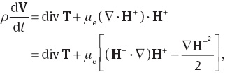
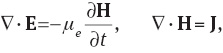
In the above equations, ς= σμ_e denotes the magnetic diffusivity, σ is the electrical conductivity, μ_e is the magnetic permeability, ρ is the density, d/dt the material derivative, T the Cauchy stress tensor, and J, E, and H the current density, the electric field, and the magnetic field respectively. The expression for T¯ is

(9)T¯ = −pI¯ + μ((grad V¯) + ((grad V¯)T)), (9)

in which I¯, p, and μ respectively, stand for the identity tensor, the pressure, and the dynamic viscosity.

Here the coordinates and velocities in the fixed (X¯, R¯, U¯, V¯) and wave frame (x¯, r¯, u¯, v¯) are related by

(10)x¯ = X¯ − ct¯,r¯ = R¯,u¯ = U¯ − c,v¯ = V¯. (10)

Employing the computations of (3)–(5) through (10), we approach at

(11)∂v¯∂r¯ + R∗r¯ +​R∗∂u¯∂x¯ + v¯r + R∗ = 0, (11)

(12)ρ[−c∂v¯∂x¯ + v¯∂v¯∂r¯ + R∗(u¯ + c)R∗ + r¯∂v¯∂x¯ − (u¯ + c)2R∗ + r¯]= −∂p¯∂r¯ + μ[1R∗ + r¯∂∂r¯{(R∗ + r¯)∂v¯∂r¯}+∂2v¯∂x¯2(R∗R ∗ + r¯)2 − v¯(r¯ + R∗)2 − 2R∗(r¯ + R∗)2∂u¯∂x¯]    −μe2(∂H+2∂r¯) + μe[(H0R∗R∗ + r¯ + h¯r¯)∂h¯r¯∂r¯ +h¯x¯R∗R∗ + r¯∂h¯r¯∂x¯ − h¯x¯2R∗ + r¯], (12)

(13)ρ[−c∂u∂x¯ + v¯∂u¯∂r¯ + R∗(u¯ + c)R∗ + r¯∂u¯∂x¯ − (u¯ + c)v¯R∗ + r¯]= −R∗R∗ + r¯∂p¯∂x¯ + μ[1R∗ + r¯∂∂r¯{(R∗ + r¯)∂u¯∂r¯}      (R∗R∗ + r¯)2∂2u¯∂x¯2 − u¯ + c(r¯ + R∗)2 − 2R∗(r¯ + R∗)2∂v¯∂x¯]    −μe2ρR∗R∗ + r¯(∂H+2∂x) + μe[(h¯x¯R∗ + r¯ + ∂h¯x¯∂r¯)     (H0R∗R∗ + r¯ + h¯r¯) + R∗R∗ + r¯h¯x¯∂h¯x¯∂x¯], (13)

where (r¯, x¯) indicates the coordinates in the wave frame. We now introduce the following quantities

(14)x = x¯λ, r = r¯a, t = ct¯λ, p = a2p¯cλμ, M2 = ReS2Rm,u = −∂ψ∂r, δ = aλ, u = u¯c, v = v¯c, k = R∗a, E = −E¯cH0μe,v = δkk + r∂ψ∂x, Re = caρμ, Rm = σμeac, S = H0cμeρ,ϕ = ϕ¯H0a, hr = δkk + r∂ϕ∂x, h¯x¯ = −ϕ¯r¯, h¯r¯ = R∗R∗ + r¯ϕ¯x¯,pm = p + 12Reδμe(H+)2ρc2, hx = −∂ϕ∂r, (14)

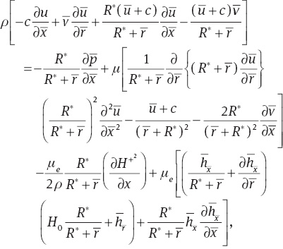
where δ, Re, R_m, S, and M are the wave, Reynolds, magnetic Reynolds, Stommer’s, and Hartman numbers, respectively. The total pressure p_m is the sum of ordinary and magnetic pressures, E is the electric field strength, ψ is the stream function, and ϕ is the magnetic force function.

We finally obtain

(15)∂p∂x = −1k∂2ψ∂r2 − (k + r)k∂3ψ∂r3 + M2E− 1k(k + r)(M2k2 − 1)∂ψ∂r + 1k(k + r), (15)

(16)∂p∂r = 0, E = kk + r∂ψ∂r + 1Rm[∂2ϕ∂r2 + 1k + r∂ϕ∂r], (16)

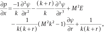
Note that a long-wavelength approximation at a low Reynolds number has been used in obtaining (15) and (16). These further give

(17)(k + r)∂4ψ∂r4 + 2∂3ψ∂r3 + (M2k2 − 1)k + r∂2ψ∂r2 − (M2k2 − 1)(k + r)2∂ψ∂r  = 1(k + r)2. (17)

The boundary conditions are

(18)Ψ = −F2, ∂Ψ∂r = 1, ϕ = 0 at y = h,Ψ = F2, ∂Ψ∂y = 1,ϕ = 0 at y = −h, (18)

where the dimensionless time mean flow rate F in the wave frame is related to the dimensionless time mean flow rate θ in the laboratory frame as

(19)θ = F + 2, F = −∫−hh∂Ψ∂rdr. (19)

3 Solution of Problem

Solving (15)–(18), we have

(20)ψ = r1 − k2M2(k + r)1 + 1 − kM21+1−kM2C1 + (k + r)1 − 1 − kM21 − 1 − kM2C2 + r(2k + r)2C3 + C4. (20)

(21)dpdx = EM2 − 1k(−1 + k2M2)(k + r)2[−2r + (−2 + b1)b1(k + r)b1C1 − (−1 + k2M2)((−2 + b2)b2 + k3M3)(k + r)b2C2 + k(−2        + (−(−2 + b1)b1 − k + k3M3) · kM2(k + r)b1C1        + (k + r)(1 + k − k(−1 + k2M2)(k + r)C3)))] (21)

(22)ϕ = 1b1kM2(−b2(k + r)b1RmC1) − 1b2kM2(b1(k + r)b2RmC2) + (E − kC3)r2 Rm + B2 − 14(−1 + k2M4){2krRm(−2 + (−1 + kM)(1 + kM)(−E + kC3)) + 2(k2(2MB1 + Rm(−2(−1 + kM)(1 + kM)(−E + kC3))) − B1ln(k + r)}. (22)

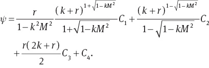
The involved C_i(i= 1–4), B_j(j= 1, 2), and b_k (k= 1, 2) are constants. The dimensionless expressions of axial induced magnetic field h_x, current density J_z, and pressure rise ΔP_λ are

(23)hx = −∂ϕ∂r, Jz = −∂2ϕ∂r2, ΔPλ = ∫01(dpdx)r = 0dx. (23)

4 Discussion

In this section, we discuss the effects of curvature k, Hartmann number M, and magnetic Reynolds number R_m appearing in the various flow quantities such as axial pressure gradient (dp/dx), pressure rise per wavelength ΔP_λ, longitudinal velocity u, axial induced magnetic field h_x, and current density J_z. We have plotted Figures 2–7 to serve the purpose.

Figure 2

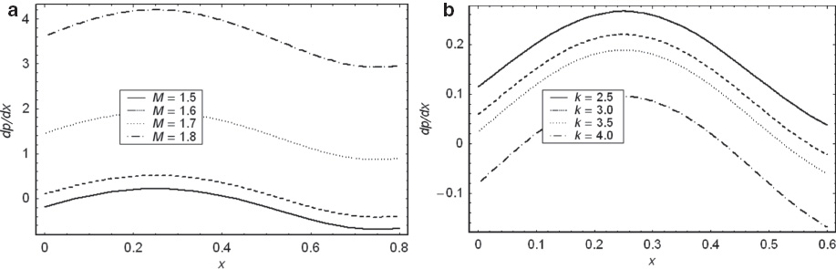
(a) The pressure gradient dp/dx versus x for α= 0.1, E= 1, k= 10 and θ= 1.5. (b) The pressure gradient dp/dx versus x for α= 0.1, E= 1, k= 1.5, and θ= 0.6.

Figure 3

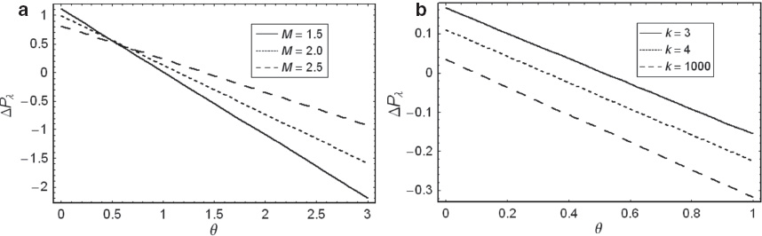
(a) The pressure rise ΔP_λ versus flow rate θ for α= 0.4, k= 2, and E= 1. (b) The pressure rise ΔP_λ versus flow rate θ for α= 0.1, M= 1.4, and E= –1.

Figure 4

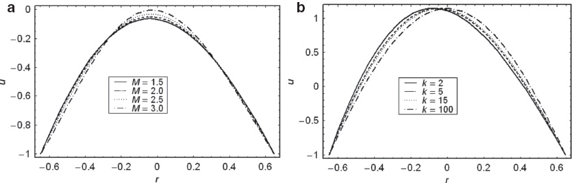
(a) The axial velocity u versus r for α= 0.6, k= 3, x= 0.6, and θ= 1.5. (b) The axial velocity u versus r for α= 0.6, M= 1.9, x= 0.6, and θ= 2.5.

Figure 5

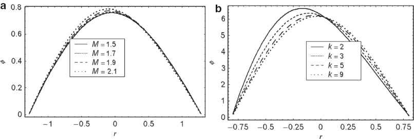
(a) The magnetic force function ϕ versus r for α= 0.3, k= 20, E= 0.8, x= 0.2, R_m= 1, and θ= –2. (b) The magnetic force function ϕ versus r for α= 0.3, k= 20, E= 0.8, x= 0.2, R_m= 1, and θ= –2.

Figure 6

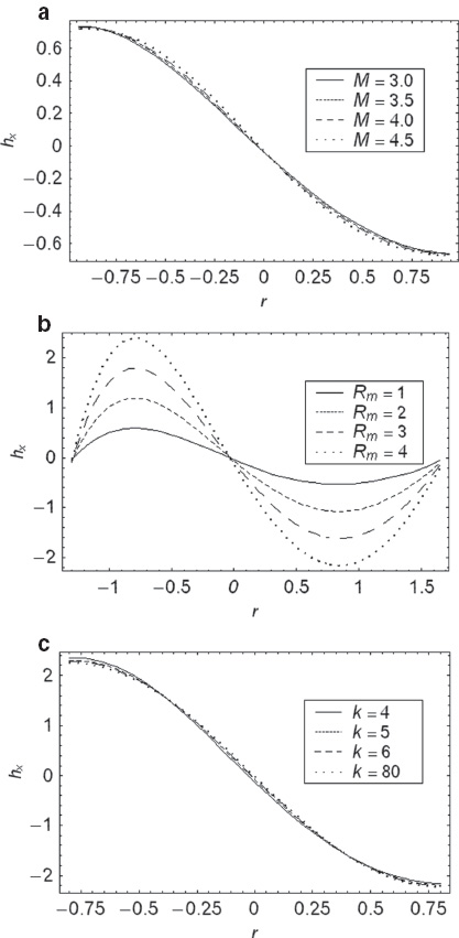
(a) The axial induced magnetic field h_x versus r for α= 0.1, M= 2.5, L= 1, R_m= 4, x= –0.2, and θ= 1. (b) The axial induced magnetic field h_x versus r for α= 0.2, M= 2.5, L= 1, k= 4, x= –0.2, and θ= 1. (c) The axial induced magnetic field h_x versus r for α= 0.1, M= 2.5, L= 1, R_m= 4, x= –0.2, and θ= 1.5.

Figure 7

(a) Current density J_z versus r for α= 0.2, R_m= 4, k= 4, x= –0.2, E= 1, and θ= 1.5. (b) Current density J_z versus r for α= 0.2, M= 1.5, k= 4, x= –0.2, E= 1, and θ= 1.5. (c) Current density J_z versus r for α= 0.2, R_m= 4, M= 2.5, x= –0.2, E= 1, and θ= 1.5.

5 Concluding Remarks

The aim of study is to obtain an analytical solution for the effects of induced magnetic field on the peristaltic transport of viscous fluid in a curved channel. The following observations have been found

• Symmetry in the profiles of u and ϕ is disturbed because of curvature effects.

• The qualitative behaviour of k and M on dp/dx is the opposite.

• ΔP_λ is a decreasing function of k and M in a curved channel.

• The magnitude of velocity u is an increasing function of k while it decreases at the centre line of the channel when M increases.

• ϕ is an increasing function of k and a decreasing function of M near the upper wall of the channel.

• Magnitude h_x increases with R_m and decreases with k and M.

• The magnitude of J_z has an increasing effect for R_m, k, and M about r= 0.

References

[1] T. W. Latham, MIT Cambridge, MA 1966.Search in Google Scholar
[2] A. H. Shapiro, M. Y. Jaffrin, and S. L. Weinberg, J. Fluid Mech. 37, 799 (1969).Search in Google Scholar
[3] T. Hayat and N. Ali, Physica A: Statistical and Theoretical Physics 371, 188 (2006).10.1016/j.physa.2006.03.059Search in Google Scholar
[4] P. Muthu, B. V. R. Kumar, and P. Chandra, Appl. Math. Model. 32, 2019 (2008).Search in Google Scholar
[5] Y. Wang, N. Ali, T. Hayat, and M. Oberlack, ASME J. Appl. Mech. 76, 011006100 (2009).Search in Google Scholar
[6] S. Srinivas and M. Kothandapani, Int. Comm. Heat Mass Transfer 35, 514 (2008).10.1016/j.icheatmasstransfer.2007.08.011Search in Google Scholar
[7] K. Vajravelu, G. Radhakrishnamacharya, and V. R. Murty, Int. J. Nonlinear Mech. 42, 754 (2007).Search in Google Scholar
[8] S. Nadeem and S. Akram, Comm. Nonlinear Sci. Numer. Simul. 15, 1705 (2010).Search in Google Scholar
[9] Abd El Hakeem Abd El Naby, J. Appl. Mech. 76, 064504 (2009).Search in Google Scholar
[10] M. H. Haroun, Comm Nonlinear Sci. Numer. Simul. 12, 1464 (2007).Search in Google Scholar
[11] D. Tripathi, Appl. Math. Comput. 215, 3645 (2010).Search in Google Scholar
[12] T. Hayat, Q. Hussain, and N. Ali, Phys. Lett. A 387, 3399 (2008).10.1016/j.physa.2008.02.040Search in Google Scholar
[13] T. Hayat, M. U. Qureshi, and N. Ali, Phys. Lett. A 372, 2653 (2008).10.1016/j.physleta.2007.12.049Search in Google Scholar
[14] T. Hayat, A. Afsar, and N. Ali, Math. Computer Modelling 47, 380 (2008).10.1016/j.mcm.2007.04.012Search in Google Scholar
[15] M. A. Abd Elnaby and M.H. Haroun, Comm. Nonlinear Sci. Numer. Simul. 13, 752 (2008).Search in Google Scholar
[16] S. Srinivas and M. Kothandapani, Appl. Math. Comput. 213, 197 (2009).Search in Google Scholar
[17? M. Kothandapani and S. Srinivas, Int. J. Non-Linear Mech. 43, 915 (2008).Search in Google Scholar
[18] Abd El Hakeem Abd El Naby, A. E. M. El Misery, and M. F. Abd El Kareem, Physica A 367, 79 (2006).10.1016/j.physa.2005.10.045Search in Google Scholar
[19] Abd El Hakeem Abd El Naby, A.E.M. El Misiery, and I. El Shamy, Appl. Math. Comput. 173, 856 (2006).Search in Google Scholar
[20] T. Hayat and N. Ali, Appl. Math. Comput. 188, 1491 (2007).Search in Google Scholar
[21] T. Hayat, N. Ahmad and N. Ali, Comm. Nonlinear Sci. Numer. Simul. 13, 1581 (2008).Search in Google Scholar
[22] T. Hayat, A. Afsar, M. Khan, and S. Asghar, Comp. Math. Applications 53, 1074 (2007).10.1016/j.camwa.2006.12.014Search in Google Scholar
[23] T. Hayat, M. Khan, A. M. Siddiqui, and S. Asghar, Comm. Nonlinear Sci. Numer. Simul. 12, 910 (2007).Search in Google Scholar
[24] T. Hayat and N. Ali, Comm. Nonlinear Sci. Numer. Simul. 13, 1343 (2008).Search in Google Scholar
[25] Kh. S. Mekheimer, Appl. Math. Comput. 153, 763 (2004).Search in Google Scholar
[26] N. T. M. Eldabe, M. F. Al-Sayad, A. Y. Galy, and H.M. Sayed, Physica A 383, 253 (2007).10.1016/j.physa.2007.05.027Search in Google Scholar
[27] V. I. Vishnyakov and K. B. Pavlov, Translated from Magnitnaya Gidrodinamika 8, 174 (1972).Search in Google Scholar
[28] Kh. S. Mekheimer, Phys. Lett. A 372, 4271 (2008).10.1016/j.physleta.2008.03.059Search in Google Scholar
[29] T. Hayat, S. Noreen, and A. Alsaedi, App. Math. Mech. 33, 1035 (2012).Search in Google Scholar
[30] T. Hayat, S. Noreen, and A. Alsaedi, J. Mech. in Med. Bio. 12, 1250058 (2012).Search in Google Scholar
[31] S. Noreen and M. Qasim, The European Physical Journal – Plus 128, 1 (2013).10.1140/epjp/i2013-13091-3Search in Google Scholar
[32] S Noreen, The European Physical Journal Plus 129, 1 (2014).10.1140/epjp/i2014-14033-3Search in Google Scholar
[33] H. Sato, T. Kawai, T. Fujita, and M. Okabe, The Japan Soc. Mech. Eng. B 66, 679 (2000).10.1299/kikaib.66.679Search in Google Scholar
[34] N. Ali, M. Sajid, and T. Hayat, Zeitschrift Fur Naturforschung A 65, 191 (2010).10.1515/zna-2010-0306Search in Google Scholar
[35] N. Ali, M. Sajid, T. Javed, and Z. Abbas, Int. J. Heat Mass Transfer 53, 3319 (2010).10.1016/j.ijheatmasstransfer.2010.02.036Search in Google Scholar
[36] N. Ali, M. Sajid, T. Javed, and Z. Abbas, Eurp. J. Mech. B/Fluids 29, 387 (2010).10.1016/j.euromechflu.2010.04.002Search in Google Scholar