Time Evolution of Some Modified Nonrelativistic Hamiltonians

1 Introduction

The Heisenberg commutation relation is supposed to be modified in the Plank length scale [1, 2]. Such modification, which is motivated by fundamental theories, such as string theory and quantum gravity, will change the mathematical form of our wave equations [1, 2]. In this field, the theoretical approaches become necessary due to the lack of a solid unified basis and experimental limitations [3, 4]. Consequently, various aspects of the problem have been analyzed so far. Das and Vagenas [3] indicated that the quantum gravity can influence almost any well-defined Hamiltonian. Maggiore and others tried to combine gravitation and quantum theory when minimal length consideration is taken into account [5–7]. In our work, we analysed the time evolution of modified nonrelativistic quantum systems of free-particle, harmonic, and linear terms. We first introduced the most essential formulae of the minimal length formulae, which is alternatively called the generalised uncertainty principle (GUP) formalism. It is well known that in the commutative formulation of quantum mechanics, the position and momentum operators satisfy the Heisenberg algebra [8]:

(1)[X^, P^] = iℏ(1 + βp^2), (1)

which corresponds to

(2)ΔX^ΔP^ ≥ ℏ2(1 + β(Δp^)2 + β < p^ >2), (2)

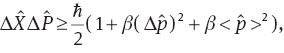
where β = β0Mplc2 = (ℓpl)22ℏ2 is a positive term, M_pl and ℓ_pl denote the Plank mass and length, respectively, M_plc² ≈ 1.2⋅10¹⁹GeV is the Plank energy [6], and we expect β₀=O(1) [8]. For β→0, (2) obviously gives the ordinary Heisenberg formula. Such a minimal length, in string theory, means that the strings cannot probe distances shorter than ℓ_pl.

For a detailed and instructive survey on various aspects of the GUP and the implications of the formalism on various interactions, the interested reader can read references provided [9–16].

2 The Time Evolution of the Modified Nonrelativistic Hamiltonian

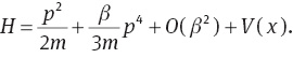
The nonrelativistic Hamiltonian in ordinary quantum mechanics has the form

(3)H^ = P^22m + V(X^), (3)

where P^, V(X^) and m represent total momentum, potential, and mass of particle, respectively. When we consider the modified Schrödinger equation, we replace the momentum and position operators with P^ = p^(1 + β3p^2), and X^ = x^ = x,p^ = p. The Hamiltonian takes the form

(4)H = p22m + β3mp4 + O(β2) + V(x). (4)

Ehrenfest’s theorem is not valid in the case of GUP [16], so we should take the classical limit by replacing commutators with Poisson brackets [17]:

(5)1iℏ[X, P] = 1 + βP2 → {X, P} = 1 + βp2, (5)

(6)1iℏ[x, p] = 1 → {x, p} = 1, (6)

We can note that the symbols without hats are c-number. This will lead to represent position and momentum operators as

{dxdt = {x, H} = {x, p22m} + {x, βp43m} = pm + 4βp33m,(7)dpdt = {p, V(x)} = −dV(x)dx,(8)

From obtained relations, we calculate time evolution in different conditions.

3 The Time Evolution of Some Modified Hamiltonians

3.1 The Free-Particle Case

It is well known that the Hamiltonian of a free particle is

(9)H = P22m, (9)

The latter, in the presence of minimal length considerations, is

(10)H = p22m + β3mp4 + O(β2), (10)

According to (7) and (8),

(11)p(t) = c1. (11)

and

(12)x(t) = c1tm + 4βc13t3m + c2. (12)

Equation (12) recovers ordinary quantum mechanics relation when β→0.

3.2 The Liner Gravitational Potential

In the free-fall motion, gravity is the only force which acts on the object. If we consider gravity force in the direction of x_-axis, the potential takes the form

(13)V(x) = mgx. (13)

and the modified Hamiltonian appears as

(14)H = p22m + β3mp4 + mgx, (14)

For this case dxdt satisfies the (7) and

(15)dpdt = {p, mgx} = −mg, (15)

From the aforementioned relation we have

(16)p(t) = −mgt + c3. (16)

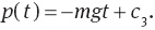
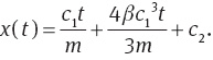
By substituting (16) into (7), we obtain

(17)dxdt = (−mgt + c3)m + 4β(−mgt + c3)33m, (17)

(18)x(t) = −12gt2 + c3mt − 13βm2g3t4 + 43βmg2c3t3 − 2βgc32t2 + 43mβc33t + c4, (18)

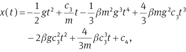
The latter, for vanishing minimal length parameter, gives the well-known relation

(19)x(t) = −12gt2 + c3mt + c4, (19)

In Figure 1 we have plotted x versus the time.

Figure 1

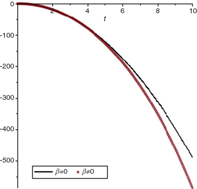
Comparison of the position in both the presence of minimal length and vanish of minimal length.

3.3 The Harmonic Oscillator

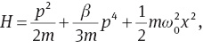
The simple harmonic oscillator potential is one of the most important problems in both classical and modern physics and possesses the Hamiltonian as (4):

(20)H = p22m + β3mp4 + 12mω02x2, (20)

dxdt is similar to (7), and according (8) one can write

(21)dpdt = {p, 12mω02x2} = −mω02x, (21)

which gives

(22)d2pdt2 = −mω02dxdt. (22)

Substitution of (7) in (22) yields the nonlinear equation

(23)d2pdt2 + ω02p = −43βω02p3. (23)

In the last section when β→0, (23) is nothing but the well-known liner harmonic oscillator equation

(24)d2pdt2 + ω02p = 0, (24)

(i.e., the minimal length has transformed the linear harmonic equation into a nonlinear counterpart). This condition enables us to use the method of successive approximations [18]. Writing

(25)−43βω02 = λ. (25)

Equation (23) is more neatly written as

(26)d2pdt2 + ω02p = λp3. (26)

We now try a first approximation of the form

(27)p(t) = A1cos(ωt). (27)

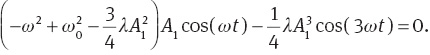
Substitution of (27) into (26) yields

(28)−A1ω2cos(ωt) + A1ω02cos(ωt) = λA13(34cos(ωt) + 14cos(3ωt)), (28)

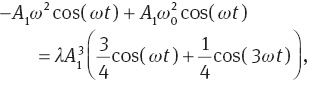
or

(29)(−ω2 + ω02 − 34λA12)A1cos(ωt) − 14λA13cos(3ωt) = 0. (29)

An approximation to ω, which is valid for small λ, is obtained by equating the first term to zero. Such a procedure gives

(30)ω = (ω02 − 34λA12)12. (30)

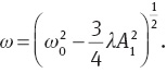
which, as we expected, gives the frequency as a function of the amplitude. The other term will lead us to add the following second term to our trial solution:

(31)p(t) = A1cos(ωt) + A3cos(3ωt). (31)

By the same token of the previous lines, we find

(32)(−ω2 + ω02 − 34λA12)A1cos(ωt) + (−9A3ω2 + ω02A3 − 14λA13)cos(3ωt)+(terms involving A3λ andcos(5ωt)) = 0. (32)

In this stage, we equate the second term to zero and obtain

(33)ω = (ω02 − 34λA12)12A3 = βA138 + 27βA13 ≈ βA138, (33)

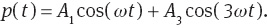
Therefore, our second approximation can be expressed as

(34)p(t) = A1cos(ωt) + βA138cos(3ωt). (34)

The solution can be improved by adding an extra term:

(35)p(t) = A1cos(ωt) + A3cos(3ωt) + A5cos(5ωt), (35)

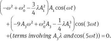
which, after some simple calculations, gives

(36)ω = (ω02 − 34λA12)12,A3 = βA138,A5 = β2A1564, (36)

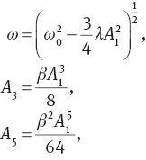
and

(37)p(t) = A1cos(ωt) + βA138cos(3ωt) + O(β2). (37)

By substituting (37) in (7) we obtain time evaluation of position operator as

(38)x(t) = A1mωsin(ωt) + 3βA13mωsin(ωt) + 3βA138mωsin(3ωt) + O(β2), (38)

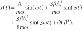
For vanishing GUP parameter, we recover the well-known sinusoidal term.

4 Conclusions

We considered the nonrelativistic time evolution of various interactions in the presence of a generalised uncertainty principle. For solving harmonic case we used the method of successive approximations and then provided an approximate analytical solution to the corresponding nonlinear equation. The solutions were reported in terms of cosine terms with arguments containing odd integer coefficients. In addition, we considered the free particle Hamiltonian and the linear term and reported the corresponding time evolution.

References

[1] H. Kragh, Am. J. Phys. 63, 595 (1995).Search in Google Scholar
[2] W. Heisenberg, Annalen der Phsik 424, 20 (1938).10.1002/andp.19384240105Search in Google Scholar
[3] S. Das and E. C. Vagenas, Can. J. Phys. 87, 233 (2009).Search in Google Scholar
[4] B. Bagchi and A. Fring, Phys. Lett. A 373, 4307 (2009).10.1016/j.physleta.2009.09.054Search in Google Scholar
[5] M. Maggiore, Phys. Lett. B 304, 65 (1993).10.1016/0370-2693(93)91401-8Search in Google Scholar
[6] M. Maggiore, Phys. Rev. D 49, 5182 (1994).10.1103/PhysRevD.49.5182Search in Google Scholar
[7] M. Maggiore, Phys. Lett. B 319, 83 (1993).10.1094/Phyto-83-319Search in Google Scholar
[8] S. Das, E. C. Vagenas, and A. F. Ali, Phys. Lett. B 690, 407 (2010).10.1016/j.physletb.2010.05.052Search in Google Scholar
[9] A. Kempf, G. Mangano, and R. B. Mann, Phys. Rev. D 52, 1108 (1995).10.1103/PhysRevD.52.1108Search in Google Scholar
[10] F. Scardigli, Phys. Lett. B 452, 39 (1999).10.1016/S0370-2693(99)00167-7Search in Google Scholar
[11] G. Amelino-Camelia, Phys. Lett. B 510, 255 (2001).10.1016/S0370-2693(01)00506-8Search in Google Scholar
[12] H. Hassanabadi, S. Zarrinkamar, and E. Maghsoodi, Phys. Lett. B 718, 678 (2012).10.1016/j.physletb.2012.11.005Search in Google Scholar
[13] T. L. Antonacci Oakes, R. O. Francisco, J. C. Fabris, and J. A. Nogueira, Eur. Phys. J. C73, 2495 (2013).10.1140/epjc/s10052-013-2495-6Search in Google Scholar
[14] S. Shams Sajadi, Eur. Phys. J. Plus 128, 57 (2013).10.1140/epjp/i2013-13057-5Search in Google Scholar
[15] H. Hassanabadi, S. Zarrinkamar, and A. A. Rajabi, Phys. Lett. B 718, 1111 (2013).10.1016/j.physletb.2012.11.044Search in Google Scholar
[16] K. Nozari and T. Azizi, Gen. Relativ. Gravit. 38, 325 (2006).Search in Google Scholar
[17] Z. Lewis, A. Roman, and T. Takeuchi, arXiv 1402,7191 (2014).Search in Google Scholar
[18] G. R. Fowles and G. L. Cassiday, Analytical Mechanics, Thomson, Washington, DC 2005.Search in Google Scholar