[go: up one dir, main page]

Next Issue
Volume 10, March
Previous Issue
Volume 10, January


Atmosphere, Volume 10, Issue 2 (February 2019) – 62 articles

Cover Story (view full-size image): 
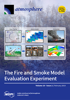
Fire and smoke models are essential tools for wildland fire decision-making and planning. The Fire and Smoke Model Evaluation Experiment (FASMEE) is designed to collect integrated observations from large wildland fires and provide evaluation datasets for existing operational systems and new model development. The campaign includes a study plan to guide the suite of required measurements in forested sites representative of many prescribed burning programs in the Southeastern US and high-intensity fires in the Western US. We provide an overview of the proposed experiment and recommendations for key measurements, which can serve as a template for additional large-scale experimental campaigns to advance fire science and operational fire and smoke models. View this paper.
  • Issues are regarded as officially published after their release is announced to the table of contents alert mailing list.
  • You may sign up for e-mail alerts to receive table of contents of newly released issues.
  • PDF is the official format for papers published in both, html and pdf forms. To view the papers in pdf format, click on the "PDF Full-text" link, and use the free Adobe Reader to open them.
Order results
Result details
Section
Select all
Export citation of selected articles as:
18 pages, 8237 KiB  
Article
Accuracy of Balloon Trajectory Forecasts in the Lower Stratosphere
by Selvaraj Dharmalingam, Riwal Plougonven, Albert Hertzog, Aurélien Podglajen, Michael Rennie, Lars Isaksen and Sélim Kébir
Atmosphere 2019, 10(2), 102; https://doi.org/10.3390/atmos10020102 - 25 Feb 2019
Cited by 5 | Viewed by 4682
Abstract
This paper investigates the accuracy of simulated long-duration super-pressure balloon trajectories in the lower stratosphere. The observed trajectories were made during the (tropical) Pre-Concordiasi and (polar) Concordiasi campaigns in 2010, while the simulated trajectories are computed using analyses and forecasts from the European [...] Read more.
This paper investigates the accuracy of simulated long-duration super-pressure balloon trajectories in the lower stratosphere. The observed trajectories were made during the (tropical) Pre-Concordiasi and (polar) Concordiasi campaigns in 2010, while the simulated trajectories are computed using analyses and forecasts from the European Centre for Medium-Range Weather Forecasts (ECMWF) Integrated Forecast System model. In contrast with the polar stratosphere situation, modelling accurate winds in the tropical lower stratosphere remains challenging for numerical weather prediction systems. The accuracy of the simulated tropical trajectories are quantified with the operational products of 2010 and 2016 in order to understand the impact of model physics and vertical resolution improvements. The median errors in these trajectories are large (typically ≳250 km after 24 h), with a significant negative bias in longitude, for both model versions. In contrast, using analyses in which the balloon-borne winds have been assimilated reduces the median error in the balloon position after 24 h to ∼60 km. For future campaigns, we describe operational strategies that take advantage of the geographic distribution and the episodic nature of large error events to anticipate the amplitude of error in trajectory forecasts. We finally stress the importance of a high vertical resolution in the model, given the intense shears encountered in the tropical lower stratosphere. Full article
(This article belongs to the Section Meteorology)
Show Figures

Figure 1

Figure 1
<p>Trajectory of Concordiasi balloon 14, from 16 October to 22 December 2010 (red). Also plotted are trajectories calculated with (<b>a</b>) OA-2010 analyses (dark blue, left panel), and (<b>b</b>) FC-2010 forecasts (cyan, right panel). Simulated trajectories are started every 6 h from the real balloon positions, and last each for three days.</p>
Full article ">Figure 2
<p>Probability Density Function (PDF) of spherical distance between the real and simulated balloon trajectories during the Concordiasi campaign with the ECMWF 2010 operational analyses (blue), and forecasts (red).</p>
Full article ">Figure 3
<p>Pre-Concordiasi balloon 1 trajectory (black line) and those calculated with winds from OA-2010 (blue), FC-2010 (cyan), CTL-2016 (purple) and BAL-2016 (green). The period depicted starts on 31 March 2010, while the real balloon is drifting eastward toward South America. Calculated trajectories shown here start every day along the real balloon flight, and last three days. Filled orange circles are shown every 24 h on the real balloon trajectories.</p>
Full article ">Figure 4
<p>Same as <a href="#atmosphere-10-00102-f003" class="html-fig">Figure 3</a>, but for the period starting on 19 March 2010.</p>
Full article ">Figure 5
<p>Probability Density Functions (PDF) of (<b>a</b>) longitudinal and (<b>b</b>) latitudinal error in the position of the simulated tropical balloons after 24 h, for trajectories calculated with winds from OA-2010 (dark blue), FC-2010 (light blue), and CTL-2016 (purple). Note that the horizontal axis covers 20°, i.e., about 2200 km, and that the PDFs in longitudes are asymmetric, in contrast to those in latitudes.</p>
Full article ">Figure 6
<p>Same as <a href="#atmosphere-10-00102-f005" class="html-fig">Figure 5</a> but for the IFS BAL-2016 setup, in which the balloon-measured winds have been assimilated. Note the difference in the horizontal-axis range when compared with <a href="#atmosphere-10-00102-f005" class="html-fig">Figure 5</a>.</p>
Full article ">Figure 7
<p>Same as <a href="#atmosphere-10-00102-f003" class="html-fig">Figure 3</a>, but for BAL-2016 trajectories computed either on model levels (dark green) or on pressure levels (light green). The vertical resolution of the archived winds is about 10 times higher on model levels than on pressure levels (250 m vs. 2.5 km).</p>
Full article ">Figure 8
<p>Vertical profiles of the zonal wind at the time and location corresponding to the first set of simulated trajectories shown in <a href="#atmosphere-10-00102-f007" class="html-fig">Figure 7</a>: OA-2010 (blue) and BAL-2016 (dark green) on model levels, as well as BAL-2016 on pressure levels (light green). The black horizontal line indicates the balloon flight level.</p>
Full article ">Figure 9
<p>Summary of the balloon trajectory errors in longitudes (<span class="html-italic">x</span>-axis) and latitudes (<span class="html-italic">y</span>-axis) after 24 h of simulation for the different IFS setups. The left panel displays the errors statistics obtained over the whole tropics, while the right panel displays those errors in different longitude ranges for the CTL-2016 and BAL-2016 setup. Shown are the 25th–75th interquartile error spreads both in longitude and latitude. The two spreads cross at the median longitudinal and latitudinal errors. The latitude scale on the <span class="html-italic">y</span>-axis is represented by horizontal (either dotted or solid) lines that are plotted every degree. Dotted lines correspond to a 0° error in latitude for the IFS setup (right panel) or longitude range (left panel) indicated along the <span class="html-italic">y</span>-axis.</p>
Full article ">Figure 10
<p>Time series of spherical distance between the real and simulated balloon positions after 24 h of simulation, for the three PreConcordiasi balloons. The simulated trajectories are calculated using the OA-2010 (top panel), CTL-2016 (middle panel) and BAL-2016 (bottom panel) IFS setups.</p>
Full article ">Figure 11
<p>Scatterplot of the error in position after 24 h (vertical axis), as a function of the error in the trajectory started 24 h earlier (horizontal axis), for simulations using CTL-2016 (purple) and for those using BAL-2016 (green). Note the logarithmic axes. The linear correlation coefficients (<span class="html-italic">R</span>) and slope of the regression line (<span class="html-italic">m</span>) in log-log space are provided in the figure.</p>
Full article ">
2 pages, 142 KiB  
Editorial
Integration of Advanced Soft Computing Techniques in Hydrological Predictions
by Kwok-wing Chau
Atmosphere 2019, 10(2), 101; https://doi.org/10.3390/atmos10020101 - 25 Feb 2019
Cited by 5 | Viewed by 2220
Abstract
Recently, extreme events have been occurring more frequently, a possible result of climate change, and have resulted in both significant economic losses as well as loss of life around the world [...] Full article
12 pages, 20934 KiB  
Article
Filtration Performance Characteristics of Sticky Aerosol Using Calcium Hydroxide
by Jae-Rang Lee, Naim Hasolli, Seong-Min Jeon, Kang-San Lee, Jun-Hyeok Gang, Kwang-Deuk Kim, Kwan-Young Lee and Young-Ok Park
Atmosphere 2019, 10(2), 100; https://doi.org/10.3390/atmos10020100 - 24 Feb 2019
Cited by 3 | Viewed by 3019
Abstract
This study examined the performance of removing aerosol upon a flow rate variable by agglomerating sticky aerosol with calcium hydroxide and removing cohesive aerosol through an experimental apparatus, simulating an actual painting booth. As a result of examining the performance of the filter [...] Read more.
This study examined the performance of removing aerosol upon a flow rate variable by agglomerating sticky aerosol with calcium hydroxide and removing cohesive aerosol through an experimental apparatus, simulating an actual painting booth. As a result of examining the performance of the filter by fixing the paint spray quantity, the calcium hydroxide input and the filtration area under variable flow rates of 5, 10, and 15 Nm3/min, we confirmed that the filter performance has long average aerosol removing intervals at the 5 Nm3/min flow rate. At the 5 Nm3/min flow rate, there is a low residual pressure drop trend and high fractional collection efficiency, and a high level of total collection efficiency is maintained at 99.42%. When the flow rate is less than 5 Nm3/min, the aerosol settling and experimentation was impossible. With this research, the optimal conditions for the use of sticky aerosol have been examined. Full article
(This article belongs to the Section Air Quality)
Show Figures

Figure 1

Figure 1
<p>1000 and 10,000 times magnified images of calcium hydroxide.</p>
Full article ">Figure 1 Cont.
<p>1000 and 10,000 times magnified images of calcium hydroxide.</p>
Full article ">Figure 2
<p>Substance analysis results of calcium hydroxide with EDS.</p>
Full article ">Figure 2 Cont.
<p>Substance analysis results of calcium hydroxide with EDS.</p>
Full article ">Figure 3
<p>The scene of a filter installed in an apparatus for the experiment.</p>
Full article ">Figure 4
<p>(<b>a</b>) Flow diagram and (<b>b</b>) scene of the actual laboratory.</p>
Full article ">Figure 4 Cont.
<p>(<b>a</b>) Flow diagram and (<b>b</b>) scene of the actual laboratory.</p>
Full article ">Figure 5
<p>Cleaning interval results with the flow rate variable.</p>
Full article ">Figure 6
<p>Residual pressure drop trend with flow rate variable.</p>
Full article ">Figure 7
<p>Cleaning efficiency results with flow rate variable.</p>
Full article ">Figure 8
<p>Total collection efficiency results with flow rate variable.</p>
Full article ">Figure 9
<p>Fractional collection efficiency results with flow rate variable.</p>
Full article ">Figure 10
<p>Photos of filters (<b>a</b>) before and (<b>b</b>) after the experiment.</p>
Full article ">Figure 11
<p>1000 times magnified photos of filter media (<b>a</b>) before and (<b>b</b>) after the experiment.</p>
Full article ">
14 pages, 1246 KiB  
Article
Evaluation of Tire Wear Contribution to PM2.5 in Urban Environments
by Julie M. Panko, Kristen M. Hitchcock, Gary W. Fuller and David Green
Atmosphere 2019, 10(2), 99; https://doi.org/10.3390/atmos10020099 - 23 Feb 2019
Cited by 96 | Viewed by 16173
Abstract
Vehicle-related particulate matter (PM) emissions may arise from both exhaust and non-exhaust mechanisms, such as brake wear, tire wear, and road pavement abrasion, each of which may be emitted directly and indirectly through resuspension of settled road dust. Several researchers have indicated that [...] Read more.
Vehicle-related particulate matter (PM) emissions may arise from both exhaust and non-exhaust mechanisms, such as brake wear, tire wear, and road pavement abrasion, each of which may be emitted directly and indirectly through resuspension of settled road dust. Several researchers have indicated that the proportion of PM2.5 attributable to vehicle traffic will increasingly come from non-exhaust sources. Currently, very little empirical data is available to characterize tire and road wear particles (TRWP) in the PM2.5 fraction. As such, this study was undertaken to quantify TRWP in PM2.5 at roadside locations in urban centers including London, Tokyo and Los Angeles, where vehicle traffic is an important contributor to ambient air PM. The samples were analyzed using validated chemical markers for tire tread polymer based on a pyrolysis technique. Results indicated that TRWP concentrations in the PM2.5 fraction were low, with averages ranging from < 0.004 to 0.10 µg/m3, representing an average contribution to total PM2.5 of 0.27%. The TRWP levels in PM2.5 were significantly different between the three cities, with significant differences between London and Los Angeles and Tokyo and Los Angeles. There was no significant correlation between TRWP in PM2.5 and traffic count. This study provides an initial dataset to understand potential human exposure to airborne TRWP and the potential contribution of this non-exhaust emission source to total PM2.5. Full article
(This article belongs to the Special Issue Air Quality and Sources Apportionment)
Show Figures

Figure 1

Figure 1
<p>Scanning electron microscope (SEM) photo of tire and road wear particles (TRWP) with characteristic morphology of tread rubber and mineral incrustations from pavement.</p>
Full article ">Figure 2
<p>Same day comparison of tire and road wear particles (TRWP) in PM2.5 between urban background site and roadside sites.</p>
Full article ">Figure 3
<p>Ratio of TRWP in PM2.5 to PM10 at sampling locations in Tokyo and London.</p>
Full article ">
3 pages, 157 KiB  
Editorial
Ocean Contributions to the Marine Boundary Layer Aerosol Budget
by Nicholas Meskhidze, Matthew Salter, Karine Sellegri and Scott Elliott
Atmosphere 2019, 10(2), 98; https://doi.org/10.3390/atmos10020098 - 23 Feb 2019
Cited by 2 | Viewed by 2836
Abstract
Projections of future climate remain an important scientific goal for much of the Earth science community [...] Full article
(This article belongs to the Special Issue Ocean Contributions to the Marine Boundary Layer Aerosol Budget)
13 pages, 5602 KiB  
Article
Plum Rain-Season-Oriented Modelling and Intervention of Indoor Humidity with and without Human Occupancy
by Jin Ye, Hua Qian, Xiaohong Zheng and Guoqing Cao
Atmosphere 2019, 10(2), 97; https://doi.org/10.3390/atmos10020097 - 22 Feb 2019
Cited by 4 | Viewed by 3831
Abstract
The plum rain season, caused by precipitation along a persistent stationary Mei-Yu front in East Asia, creates favorable temperatures and relative humidity (RH) for mold growth indoors. This paper investigates the effects of human occupancy on indoor humidity and investigates the [...] Read more.
The plum rain season, caused by precipitation along a persistent stationary Mei-Yu front in East Asia, creates favorable temperatures and relative humidity (RH) for mold growth indoors. This paper investigates the effects of human occupancy on indoor humidity and investigates the efficient RH reduction methods to prevent mold growth in moist climates. The research is carried out based on a case study which compares a family-occupied home and another unoccupied one during typical plum rain season in Nanjing. Firstly, by analyzing the factors that can influence the indoor air RH, this paper develops a comprehensive model to evaluate the efficiency of various RH intervention methods. Secondly, this paper collects the meteorological data in Nanjing at different time scales, from days to hours. Thirdly, a specific case study is carried out based on the model and data. The results show that dehumidification and heating can always reduce RH below the critical value under which the mold growth could be inhibited. However, the effects of ventilation are more sophisticated and depend upon the human occupancy, outdoor air temperature, and air change per hour (ACH). In certain unoccupied cases, the ventilation may be inappropriate and may continuously bring moisture outside into the indoor environment, which has adverse effects on mold suppression. In the occupied cases, the condition changes significantly because the human is deemed as an internal source of heat and moist. Special care should be exercised for occupied ventilation in order to determine the optimal ACH and appropriate outdoor temperatures. Finally, some guidance is given to prevent mold growth in the general area that suffers from the plum rain season. Full article
Show Figures

Figure 1

Figure 1
<p>The critical relative humidity (RH) for mold growth on a wooden material [<a href="#B9-atmosphere-10-00097" class="html-bibr">9</a>].</p>
Full article ">Figure 2
<p>The sketch map of an ordinary home occupied with parents and one child.</p>
Full article ">Figure 3
<p>Outdoor air temperature (<b>A</b>) and <span class="html-italic">RH</span> (<b>B</b>) during the plum rain season in Nanjing in 2015.</p>
Full article ">Figure 3 Cont.
<p>Outdoor air temperature (<b>A</b>) and <span class="html-italic">RH</span> (<b>B</b>) during the plum rain season in Nanjing in 2015.</p>
Full article ">Figure 4
<p>The diurnal variation of outdoor air temperature and <span class="html-italic">RH</span> on a plum rain day.</p>
Full article ">Figure 5
<p>Diurnal variation of outdoor and indoor air temperature.</p>
Full article ">Figure 6
<p>Diurnal variation of outdoor and indoor air RH.</p>
Full article ">Figure 7
<p>Indoor air temperature in the unoccupied home (<b>A</b>) and occupied home (<b>B</b>).</p>
Full article ">Figure 7 Cont.
<p>Indoor air temperature in the unoccupied home (<b>A</b>) and occupied home (<b>B</b>).</p>
Full article ">Figure 8
<p>The highest indoor air <span class="html-italic">RH</span> with different ventilation rates.</p>
Full article ">Figure 9
<p>The highest indoor air <span class="html-italic">RH</span> under various outdoor air temperatures in the occupied home.</p>
Full article ">Figure 10
<p>The highest indoor air <span class="html-italic">RH</span> under different dehumidification rates.</p>
Full article ">Figure 11
<p>The highest indoor air <span class="html-italic">RH</span> under different heating rates in the unoccupied home.</p>
Full article ">
16 pages, 562 KiB  
Article
Characterization of Human Health Risks from Particulate Air Pollution in Selected European Cities
by Eleftheria Chalvatzaki, Sofia Eirini Chatoutsidou, Heli Lehtomäki, Susana Marta Almeida, Konstantinos Eleftheriadis, Otto Hänninen and Mihalis Lazaridis
Atmosphere 2019, 10(2), 96; https://doi.org/10.3390/atmos10020096 - 21 Feb 2019
Cited by 64 | Viewed by 5836
Abstract
The objective of the current study was to estimate health risk indexes caused by the inhalation of particulate matter (PM) by adult males and children using data sampled in three European cities (Athens, Kuopio, Lisbon). Accordingly, the cancer risk (CR) and the hazard [...] Read more.
The objective of the current study was to estimate health risk indexes caused by the inhalation of particulate matter (PM) by adult males and children using data sampled in three European cities (Athens, Kuopio, Lisbon). Accordingly, the cancer risk (CR) and the hazard quotient (HQ) were estimated from particle-bound metal concentrations whilst the epidemiology-based excess risk (ER), the attributable fraction (AF), and the mortality cases were obtained due to exposure to PM10 and PM2.5. CR and HQ were estimated using two methodologies: the first methodology incorporated the particle-bound metal concentrations (As, Cd, Co, Cr, Mn, Ni, Pb) whereas the second methodology used the deposited dose rate of particle-bound metals in the respiratory tract. The indoor concentration accounts for 70% infiltration from outdoor air for the time activity periods allocated to indoor environments. HQ was lower than 1 and the cumulative CR was lower than the acceptable level (10−4), although individual CR for some metals exceeded the acceptable limit (10−6). In a lifetime the estimated number of attributable cancer cases was 74, 0.107, and 217 in Athens, Kuopio, and Lisbon, respectively. Excess risk-based mortality estimates (due to outdoor pollution) for fine particles were 3930, 44.1, and 2820 attributable deaths in Athens, Kuopio, and Lisbon, respectively. Full article
(This article belongs to the Section Aerosols)
Show Figures

Figure 1

Figure 1
<p>Cancer risk for (<b>a</b>) adult males and (<b>b</b>) children estimated from both methodologies for each metal and city.</p>
Full article ">
10 pages, 3155 KiB  
Article
Spatial and Temporal Variations of Compound Droughts and Hot Extremes in China
by Xinying Wu, Zengchao Hao, Fanghua Hao, Chong Li and Xuan Zhang
Atmosphere 2019, 10(2), 95; https://doi.org/10.3390/atmos10020095 - 21 Feb 2019
Cited by 39 | Viewed by 4955
Abstract
Droughts and hot extremes may lead to tremendous impacts on the ecosystem and different sectors of the society. A variety of studies have been conducted on the variability of the individual drought or hot extreme in China. However, the evaluation of compound droughts [...] Read more.
Droughts and hot extremes may lead to tremendous impacts on the ecosystem and different sectors of the society. A variety of studies have been conducted on the variability of the individual drought or hot extreme in China. However, the evaluation of compound droughts and hot extremes, which may induce even larger impacts than the individual drought or hot extreme, is still lacking. The aim of this study is to investigate changes in the frequency and spatial extent of compound droughts and hot extremes during summer in China using monthly precipitation and daily temperature data from 1953 to 2012. Results show that a high frequency of compound droughts and hot extremes mostly occur in the regions stretching from northeast to southwest of China. There is an overall increase in the frequency of co-occurrence of droughts and hot extremes across most parts of China with distinct regional patterns. In addition, an increasing trend in the areas covered by compound extremes has been observed, especially after the 1990s. At regional scales, the increase of the frequency and spatial extent of compound extremes has been shown to be most profound in North China (NC), South China (SC), and Southwest China (SWC), while the decrease of compound extremes was found in Central China (CC). These results show the variability of compound droughts and hot extremes and could provide useful insights into the mitigation efforts of extreme events in China. Full article
(This article belongs to the Special Issue Weather and Climate Extremes: Current Developments)
Show Figures

Figure 1

Figure 1
<p>The study area of seven regions in China.</p>
Full article ">Figure 2
<p>The frequency (days) of compound droughts (SPI) and hot extremes (NHD) based on the threshold SPI &lt; −0.8 ((<b>A</b>): SPI3, (<b>B</b>): SPI6) and the correlation between SPI and NHD (<b>C</b>): SPI3, (<b>D</b>): SPI6) over the period 1953–2012 in China.</p>
Full article ">Figure 3
<p>Changes in the frequency (days) of compound droughts and hot extremes for the period 1983–2012 relative to 1953–1982 based on SPI3 and SPI6 using two thresholds −0.5 and −0.8. (<b>A</b>): SPI3 &lt; −0.5, (<b>B</b>): SPI6 &lt; −0.5, (<b>C</b>): SPI3 &lt; −0.8, (<b>D</b>): SPI6 &lt; −0.8.</p>
Full article ">Figure 4
<p>Changes in the spatial extent of drought (SPI), hot extreme (NHD) and compound droughts and hot extremes (SPI&amp;NHD) during 1953–2012 in China based on different time scales and thresholds of SPI. (<b>A</b>): SPI3 &lt; −0.5; (<b>B</b>): SPI6 &lt; −0.5; (<b>C</b>): SPI3 &lt; −0.8; (<b>D</b>): SPI6 &lt; −0.8.</p>
Full article ">Figure 5
<p>Changes in the frequency (days) of compound droughts and hot extremes for the two periods 1983–2012 and 1953–1982 for different regions in China. (<b>A</b>): SPI3 &lt; −0.5; (<b>B</b>): SPI6 &lt; −0.5; (<b>C</b>): SPI3 &lt; −0.8; (<b>D</b>): SPI6 &lt; −0.8.</p>
Full article ">
20 pages, 6771 KiB  
Article
Identification of Drought Events and Correlations with Large-Scale Ocean–Atmospheric Patterns of Variability: A Case Study in Xinjiang, China
by Junqiang Yao, Dilinuer Tuoliewubieke, Jing Chen, Wen Huo and Wenfeng Hu
Atmosphere 2019, 10(2), 94; https://doi.org/10.3390/atmos10020094 - 21 Feb 2019
Cited by 36 | Viewed by 4429
Abstract
This research analyzed the spatiotemporal patterns of drought in Xinjiang (northwestern China) between 1961 and 2015 using the standardized precipitation evapotranspiration index (SPEI). Furthermore, the correlations between Atlantic Multidecadal Oscillation (AMO)/El Niño–Southern Oscillation (ENSO) events and drought were explored. The results suggested an [...] Read more.
This research analyzed the spatiotemporal patterns of drought in Xinjiang (northwestern China) between 1961 and 2015 using the standardized precipitation evapotranspiration index (SPEI). Furthermore, the correlations between Atlantic Multidecadal Oscillation (AMO)/El Niño–Southern Oscillation (ENSO) events and drought were explored. The results suggested an obvious trend toward aggravated drought, with a significant inflection point in 1997, after which the frequency of drought increased sharply. Spatially, the increase in drought occurred largely in southern and eastern Xinjiang, where occurrences of moderate and extreme drought have become more frequent during the last two decades, whereas northwestern Xinjiang and the Pamir Plateau showed wetting trends. Empirical orthogonal function analysis (EOF) of drought patterns showed a north–south antiphase and an east–west antiphase distribution. The positive (negative) phase of the AMO was related to increased (decreased) drought in Xinjiang, particularly after 1997. During a warm phase (El Niño), major droughts occurred over northern Xinjiang, but they lagged by 12 months. However, not all El Niño and La Niña events were responsible for drought events in northern Xinjiang during this period, and other drivers remain to be identified. This study suggests the possibility of AMO and ENSO links to drought in Xinjiang, but further analysis is needed to better understand such mechanisms. Full article
(This article belongs to the Special Issue Meteorological and Hydrological Droughts)
Show Figures

Graphical abstract

Graphical abstract
Full article ">Figure 1
<p>Study area and meteorological stations in Xinjiang.</p>
Full article ">Figure 2
<p>(<b>a</b>) Temporal variability (straight lines denote linear trend) and (<b>b</b>) M–K test of annual SPEI for 1961–2015 in Xinjiang. The UF curve indicates the statistical series of the standard normal distribution, and the UB curve indicates the reverse statistical series. Because the line UF is above the confidence line (<span class="html-italic">p</span> = 0.05, green line), the crossing point of UF and UB is the start of abrupt change in this series.</p>
Full article ">Figure 3
<p>Interannual variability of SPEI at different timescales in (<b>a</b>) North Xinjiang and (<b>b</b>) South Xinjiang (the vertical axis represents the timescale from 1 to 24 months, and the horizontal axis represents the year from 1961 to 2015).</p>
Full article ">Figure 4
<p>(<b>a</b>) Frequency of drought and wetness variability before and after 1997. Spatial distributions of drought frequency difference (DFD) between 1997–2015 and 1961–1996 in Xinjiang: (<b>b</b>) mild drought, (<b>c</b>) moderate drought, and (<b>d</b>) extreme drought. DFD is defined as the average annual number of drought months with a category different from the average (units: times per year, 1997–2015 minus 1961–1996).</p>
Full article ">Figure 5
<p>First three loading vectors and their corresponding principal component (PC) series for 1961–2015. (<b>a1</b>–<b>c1</b>) empirical orthogonal function (EOF) analysis for annual SPEI; (<b>a2</b>–<b>c2</b>) corresponding PCs for annual SPEI.</p>
Full article ">Figure 6
<p>Changes in (<b>a</b>) magnitude, (<b>b</b>) intensity, and (<b>c</b>) percentage of stations affected with duration of drought events.</p>
Full article ">Figure 7
<p>1962–2015 monthly SPEI at 12 time scales (<b>a</b>, red line indicates the 121 month smoothed SPEI index) and the Atlantic Multidecadal Oscillation (AMO) index (<b>b</b>, blue line indicates the 121 month smoothed AMO index).</p>
Full article ">Figure 8
<p>(<b>a</b>) 1962–2015 monthly SPEI at 12 time scales and (<b>b</b>) sea surface temperature (SST) anomaly (for Niño3.4) and their low-pass variability after applying a 60-month (5-year) running mean (shaded). Yellow areas correspond to periods of drought and negative SST anomaly. (<b>c</b>) Cross correlation between Niño 3.4 SST anomaly and SPEI with negative lags for SST leading SPEI.</p>
Full article ">Figure A1
<p>Scale plot of annual eigenvalues versus eigenvector number for annual SPEI: (<b>a</b>) 1961–2015; (<b>b</b>) 1997–2015.</p>
Full article ">Figure A2
<p>First three loading vectors and their corresponding PCs series for 1997–2015: (<b>a1</b>–<b>c1</b>) EOF analysis for annual SPEI; (<b>a2</b>–<b>c2</b>) corresponding PCs for annual SPEI.</p>
Full article ">Figure A3
<p>(<b>a</b>) Spatial distribution of the cumulative SPEI value and the intensity; (<b>b</b>) percentage of stations affected from May 2008 to December 2009.</p>
Full article ">Figure A4
<p>(<b>a</b>) Temporal variation of AMO and PC1 during 1961–2015, where the red histogram represents the positive phase of AMO (AMO+) and the blue histogram represents the negative phase (AMO−); (<b>b</b>) temporal variation of the AMO and PC2 during 1961–2015.</p>
Full article ">Figure A5
<p>Spatial distribution of the correlation coefficient (CC) between (<b>a</b>) AMO and SPEI for 1961–2015 and (<b>b</b>) between ENSO and SPEI during 1997–2015.</p>
Full article ">
24 pages, 4713 KiB  
Article
Assessing the Performance of CMIP5 GCMs for Projection of Future Temperature Change over the Lower Mekong Basin
by Yunfeng Ruan, Zhaofei Liu, Rui Wang and Zhijun Yao
Atmosphere 2019, 10(2), 93; https://doi.org/10.3390/atmos10020093 - 21 Feb 2019
Cited by 24 | Viewed by 4466
Abstract
In this study, we assessed the performance of 34 Coupled Model Intercomparison Project Phase 5 (CMIP5) general climate models (GCMs) for simulating the observed temperature over the Lower Mekong Basin (LMB) in 1961–2004. An improved score-based method was used to rank the performance [...] Read more.
In this study, we assessed the performance of 34 Coupled Model Intercomparison Project Phase 5 (CMIP5) general climate models (GCMs) for simulating the observed temperature over the Lower Mekong Basin (LMB) in 1961–2004. An improved score-based method was used to rank the performance of the GCMs over the LMB. Two methods of multi-model ensemble (MME), sub-ensemble from the top 25% ranked GCMs and full ensemble from the entire GCMs, were calculated using arithmetic mean (AM) method and downscaled using the Delta method to project future temperature change during two future time periods, the near future (2006–2049) and the far future (2050–2093), under representative concentration pathways (RCP2.6, RCP4.5, and RCP8.5 scenarios) over the LMB. The improved score-based method combining multiple criteria showed a robust assessment of the GCMs performance over the LMB, which can provide good information for projecting future temperature change. The results showed a significant increase in temperature over the LMB under the two ensembles. However, there were differences in the magnitudes of the future temperature increase between the two ensemble methods, with a higher mean annual temperature increase from full ensemble and sub-ensemble at 1.26 °C (1.09 °C), 1.90 °C (1.70 °C), and 2.97 °C (2.78 °C) during 2050–2093 under the RCP2.6, RCP4.5, and RCP8.5 scenarios compared to the values at 0.93 °C (0.87 °C), 0.99 °C (0.95 °C), and 1.09 °C (1.06 °C) during 2006–2049, respectively, relative to the reference time period of 1961–2004. In the future (2006–2093), the temperature is likely to increase at 0.06 °C, 0.18 °C, and 0.39 °C decade−1 under the RCP2.6, RCP4.5, and RCP8.5 scenarios by the sub-ensemble, while a higher temperature increase at 0.08 °C, 0.20 °C, and 0.42 °C was found by the full ensemble over the LMB, relative to the reference time period of 1961–2004. On the whole, the higher warming mainly occurred in the northern and central areas over the LMB, while the lower warming mainly occurred in the southeast and the southwest, especially under the RCP4.5 and RCP8.5 scenarios, with the warming increased with increasing RCP for both ensembles. Moreover, in order to reduce the uncertainty of temperature projection in further studies in the LMB, multiple methods of GCMs ensemble should be considered and compared. Full article
(This article belongs to the Section Meteorology)
Show Figures

Figure 1

Figure 1
<p>Location of the Lower Mekong Basin (LMB) and the 21 selected grids (shade of yellow) over the LMB.</p>
Full article ">Figure 2
<p>Variation of the observed temperature and GCMs of the mean annual cycle during the reference period 1961–2004 over the LMB.</p>
Full article ">Figure 3
<p>Ranking scores of criteria of the GCMs over the LMB.</p>
Full article ">Figure 4
<p>Ascending order of ranking scores for the performance of the GCMs over the LMB.</p>
Full article ">Figure 5
<p>Comparison of overall RS (ranking scores) and RS after removing one criterion. The numbers in the X axis represent the ID numbers in <a href="#atmosphere-10-00093-t001" class="html-table">Table 1</a>.</p>
Full article ">Figure 6
<p>Comparison of overall ranking scores of GCMs under reference periods of 1975–2004 and 1961–2004 (<b>a</b>) and top 25% ranking scores of GCMs under reference period of 1975–2004 (<b>b</b>) and 1961–2004 (<b>c</b>), respectively. The numbers on the x-axis (<b>a</b>) represent the ID numbers in <a href="#atmosphere-10-00093-t001" class="html-table">Table 1</a>.</p>
Full article ">Figure 7
<p>Future temperature changes for RCP2.6, RCP4.5, and RCP8.5 scenarios relative to the period of 1961–2004 over the LMB under two ways of multi-model ensemble after smoothing with five years moving average. The red lines represent the mean values of all the grids. The shaded areas represent the values of variation range of all the grids. The dotted line represents the linear regression. The degrees of freedom (DOF) are all 83 for the RCP2.6, RCP4.5, and RCP8.5 scenarios.</p>
Full article ">Figure 8
<p>Changes in mean annual temperature (°C) over the LMB during 2006–2049 and 2050–2093 relative to the reference period of 1961–2004 under RCP2.6, RCP4.5, and RCP8.5 scenarios from two ensemble methods.</p>
Full article ">Figure 9
<p>Changes in mean MAM temperature (°C) over the LMB during 2006–2049 and 2050–2093 relative to the reference period of 1961–2004 RCP2.6, RCP4.5, and RCP8.5 scenarios from two ensemble methods.</p>
Full article ">Figure 10
<p>Changes in mean JJA temperature (°C) over the LMB during 2006–2049 and 2050–2093 relative to the reference period of 1961–2004 RCP2.6, RCP4.5, and RCP8.5 scenarios from two ensemble methods.</p>
Full article ">Figure 11
<p>Changes in mean SON temperature (°C) over the LMB during 2006–2049 and 2050–2093 relative to the reference period of 1961‒2004 RCP2.6, RCP4.5, and RCP8.5 scenarios from two ensemble methods.</p>
Full article ">Figure 12
<p>Changes in mean DJF temperature (°C) over the LMB during 2006–2049 and 2050–2093 relative to the reference period of 1961–2004 RCP2.6, RCP4.5, and RCP8.5 scenarios from two ensemble methods.</p>
Full article ">
19 pages, 1127 KiB  
Article
Changes in Global Blocking Character in Recent Decades
by Anthony R. Lupo, Andrew D. Jensen, Igor I. Mokhov, Alexander V. Timazhev, Timothy Eichler and Bahtiyar Efe
Atmosphere 2019, 10(2), 92; https://doi.org/10.3390/atmos10020092 - 21 Feb 2019
Cited by 50 | Viewed by 4271
Abstract
A global blocking climatology published by this group for events that occurred during the late 20th century examined a comprehensive list of characteristics that included block intensity (BI). In addition to confirming the results of other published climatologies, they found that Northern Hemisphere [...] Read more.
A global blocking climatology published by this group for events that occurred during the late 20th century examined a comprehensive list of characteristics that included block intensity (BI). In addition to confirming the results of other published climatologies, they found that Northern Hemisphere (NH) blocking events (1968–1998) were stronger than Southern Hemisphere (SH) blocks and winter events are stronger than summer events in both hemispheres. This work also examined the interannual variability of blocking as related to El Niño and Southern Oscillation (ENSO). Since the late 20th century, there is evidence that the occurrence of blocking has increased globally. A comparison of blocking characteristics since 1998 (1998–2018 NH; 2000–2018 SH) shows that the number of blocking events and their duration have increased significantly in both hemispheres. The blocking BI has decreased by about six percent in the NH, but there was little change in the BI for the SH events. Additionally, there is little or no change in the primary genesis regions of blocking. An examination of variability related to ENSO reveals that the NH interannual-scale variations found in the earlier work has reversed in the early 21st century. This could either be the result of interdecadal variability or a change in the climate. Interdecadal variations are examined as well. Full article
(This article belongs to the Section Meteorology)
Show Figures

Figure 1

Figure 1
<p>The number of block onsets per year versus longitude where the left-hand side begins with 180° longitude for the (<b>a</b>) [<a href="#B1-atmosphere-10-00092" class="html-bibr">1</a>] study, (<b>b</b>) the current study period, and (<b>c</b>) the difference between (<b>b</b>) and (<b>a</b>).</p>
Full article ">Figure 2
<p>As in <a href="#atmosphere-10-00092-f001" class="html-fig">Figure 1</a>, except for the SH.</p>
Full article ">Figure 3
<p>The occurrence of blocking for (<b>a</b>) the NH, and (<b>b</b>) the SH with time. The blue dashed line is a linear trend line, while the green dashed line is a quadratic fit.</p>
Full article ">Figure 4
<p>A spectral analysis of the time series for (<b>a</b>) NH (left) and (<b>b</b>) SH (right) block occurrences. The dotted line is the 95% confidence level assuming a white noise spectrum, while the green dashed line assumes a red noise spectrum (see [<a href="#B52-atmosphere-10-00092" class="html-bibr">52</a>]). The abscissa is cycles per decade and the ordinate is spectral power.</p>
Full article ">
14 pages, 4847 KiB  
Article
Dry-Heat Cooking of Meats as a Source of Airborne N-Nitrosodimethylamine (NDMA)
by Hekap Kim, Jiyeon Tcha, Man-yong Shim and Sungjin Jung
Atmosphere 2019, 10(2), 91; https://doi.org/10.3390/atmos10020091 - 20 Feb 2019
Cited by 3 | Viewed by 5834
Abstract
This study aimed to investigate the airborne release of N-nitrosodimethylamine (NDMA) as a result of the dry-heat cooking of some meats using charcoal grilling and pan-broiling methods. Three types of meat (beef sirloin, pork belly, and duck) were chosen and cooked in [...] Read more.
This study aimed to investigate the airborne release of N-nitrosodimethylamine (NDMA) as a result of the dry-heat cooking of some meats using charcoal grilling and pan-broiling methods. Three types of meat (beef sirloin, pork belly, and duck) were chosen and cooked in a temporary building using the above methods. Air samples were collected in Thermosorb-N cartridges, which were qualitatively and quantitatively analyzed for NDMA using ultra-high performance liquid chromatography–mass spectrometry and high-performance liquid chromatography–fluorescence detection, respectively. Overall, the charcoal grilling method showed higher average NDMA concentrations than the pan-broiling method for all types of meat. The highest average concentration was observed for charcoal-grilled beef sirloin (410 ng/m3) followed by pork belly, suggesting that meat protein content and cooking duration are important determinants of NDMA formation. Cancer risk assessment showed that the charcoal grilling of such meats can pose an additional cancer risk for restaurant customers. Full article
(This article belongs to the Special Issue Indoor Air Pollution)
Show Figures

Graphical abstract

Graphical abstract
Full article ">Figure 1
<p>A schematic diagram of the temporary building in which the charcoal grilling and pan-broiling experiments were conducted.</p>
Full article ">Figure 2
<p>A schematic diagram of an experimental setting for air sampling during the charcoal grilling experiments.</p>
Full article ">Figure 3
<p>Selected reaction monitoring chromatograms (left) and mass spectra (right) for the seven nitrosamine standard solutions (2 ng/L) recorded using ultra-performance liquid chromatography-mass/mass (UPLC-MS/MS).</p>
Full article ">Figure 4
<p>A selected reaction monitoring chromatogram (top) and a mass spectrum (bottom) for <span class="html-italic">N</span>-nitrosodimethylamine (NDMA), the only nitrosamine identified in air samples, recorded using UPLC-MS/MS.</p>
Full article ">Figure 5
<p>Chromatograms of a 200 ng/m<sup>3</sup> <span class="html-italic">N</span>-nitrosamine standard (top) and an air sample (bottom).</p>
Full article ">
13 pages, 2672 KiB  
Article
Climatic Effects of China Large-Scale Urbanization on East Asian Summer Monsoon under Different Phases of Pacific Decadal Oscillation
by Yongxiao Liang and Pengfeng Xiao
Atmosphere 2019, 10(2), 90; https://doi.org/10.3390/atmos10020090 - 20 Feb 2019
Cited by 1 | Viewed by 2863
Abstract
The effects of urbanization over eastern China on the East Asian summer monsoon (EASM) under different sea surface temperature background are compared using a Community Atmosphere Model (CAM5.1). Experiments of urbanization investigated by comparing two climate simulations with and without urban land cover [...] Read more.
The effects of urbanization over eastern China on the East Asian summer monsoon (EASM) under different sea surface temperature background are compared using a Community Atmosphere Model (CAM5.1). Experiments of urbanization investigated by comparing two climate simulations with and without urban land cover under both positive and negative phases of Pacific Decadal Oscillation (PDO) show the spatial distribution of precipitation with ‘southern flood and northern drought’ and weakening status of EASM. The climate effect of urbanization in eastern China is significantly different from north to south. Anomalous vertical ascending motion due to the role of urbanization in the south of 30° N have induced an increase in convective available potential energy (CAPE) and precipitation increase over southern China. At the same time, the downward vertical motion occurs in the north of 30° N which cause warming over northern China. Due to the anti-cyclonic anomalies in the upper and lower layers of the north, the monsoon circulation is weakened which can reduce the precipitation. However, urbanization impact under various phases of PDO show different effect. In the 1956–1970 urbanization experiments of negative PDO phase, the downward vertical motion and anti-cyclonic anomalies in the north of 30° N are also weaker than that of positive phase of PDO in 1982–1996. In terms of this situation, the urbanization experiments of negative phase of PDO reveal that the range of the warming area over the north of 40° N is small, and the warming intensity is weak, but the precipitation change is more obvious compared with the background of positive phase of PDO. Full article
(This article belongs to the Section Meteorology)
Show Figures

Figure 1

Figure 1
<p>(<b>a</b>) Percentage distribution of urban land-cover fraction in control runs of CAM5.1 model (unit: %). The black rectangle shows the major urban agglomeration over eastern China. The urban land cover were removed in experiments of NoU_P and NoU_N; (<b>b</b>) The meta data of PDO index derived as the leading principle component (PC) of monthly SST [<a href="#B14-atmosphere-10-00090" class="html-bibr">14</a>] anomalies in the North Pacific Ocean, poleward of 20° N. The monthly mean global average SST anomalies were removed to separate this pattern of variability from any “global warming” signal that may be present in the data. Here shows the JJA (June, July, and August) average which is the result of 15-year running mean.</p>
Full article ">Figure 2
<p>Taylor assessment chart (model results and observations). (<b>a</b>) CTL_N; (<b>b</b>) CTL_P. The red dots represent the 2-m air temperature, green dots represent zonal wind in 850 hPa, blue dots represent meridional wind in 850 hPa, and orange dots represent precipitation. The domain for East Asia is 20–60° N, 110–140° E.</p>
Full article ">Figure 3
<p>Spatial evaluation between observation and CAM output over 1982–1996. (<b>a</b>,<b>d</b>,<b>g</b>), (<b>b</b>,<b>e</b>,<b>h</b>) represent the result of observation (model output) for temperature (units: °C), precipitation (units: mm/day), and low-level circulation (units: m/s). (<b>a</b>,<b>d</b>,<b>g</b>) were based on NCEP1 reanalysis data. (<b>c</b>,<b>f</b>,<b>i</b>) show the difference between CAM5.1 output and observation.</p>
Full article ">Figure 4
<p>The difference fields (CTL_P minus NoU_P and CTL_N minus NoU_N) for 2-m air-temperature (<b>a</b>,<b>b</b>; units: °C) and precipitation (<b>c</b>,<b>d</b>; units: mm/day). (<b>a</b>,<b>b</b>) use the SST of 1982–1996 (CTL_P minus NoU_P), and (<b>c</b>,<b>d</b>) use the SST of 1956–1970 (CTL_N minus NoU_N). The stippled area indicates above 90% confidence level, and relatively concentrated urban area is marked by the black rectangle.</p>
Full article ">Figure 5
<p>Difference fields (CTL_P minus NoU_P and CTL_N minus NoU_N) of wind vectors on 850 hPa (<b>a</b>,<b>b</b>; units: m/s) and 200 hPa (<b>c</b>,<b>d</b>; units: m/s). (<b>a</b>,<b>b</b>) use the SST of 1982–1996, and (<b>c</b>,<b>d</b>) use the SST of 1956–1970. Above 90% confidence level of wind speed has been shaded.</p>
Full article ">Figure 6
<p>Possible mechanism of urbanization impact on climate based on different PDO phases. Left column: 1982–1996; right column: 1956–1970. (<b>a</b>,<b>b</b>) show the surface wind of difference between CTL_P and NoU_P, and CTL_N and NoU_N, respectively. (<b>c</b>–<b>h</b>) show vertical-meridional cross-sections of the difference between CTL_P and NoU_P, and CTL_N and NoU_N, respectively. (<b>c</b>,<b>d</b>) show adiabatic heating of dry air (shading; K day<sup>−1</sup>). (<b>e</b>,<b>f</b>) show temperature (shading; °C), specific humidity (contour; g/kg) and vertical velocity (vector; revealed by (v, −ω), where v (m s<sup>−1</sup>) is meridional velocity and –ω (10<sup>−2</sup> Pa s<sup>−1</sup>) represents vertical pressure velocity) averaged over 110°–122° E. (<b>g</b>,<b>h</b>) show the difference field between CTL and NOURBAN of zonal wind (shading; m/s) and climatological zonal wind which is averaged over 110°–122° E. Above 90% confidence level of wind speed has been shaded. The stippled area shows above 90% confidence level of adiabatic heating of dry air, ω, and zonal velocity. The slash lines show above 90% confidence level of temperature. The horizontal lines show above 90% confidence level of specific humidity.</p>
Full article ">Figure 6 Cont.
<p>Possible mechanism of urbanization impact on climate based on different PDO phases. Left column: 1982–1996; right column: 1956–1970. (<b>a</b>,<b>b</b>) show the surface wind of difference between CTL_P and NoU_P, and CTL_N and NoU_N, respectively. (<b>c</b>–<b>h</b>) show vertical-meridional cross-sections of the difference between CTL_P and NoU_P, and CTL_N and NoU_N, respectively. (<b>c</b>,<b>d</b>) show adiabatic heating of dry air (shading; K day<sup>−1</sup>). (<b>e</b>,<b>f</b>) show temperature (shading; °C), specific humidity (contour; g/kg) and vertical velocity (vector; revealed by (v, −ω), where v (m s<sup>−1</sup>) is meridional velocity and –ω (10<sup>−2</sup> Pa s<sup>−1</sup>) represents vertical pressure velocity) averaged over 110°–122° E. (<b>g</b>,<b>h</b>) show the difference field between CTL and NOURBAN of zonal wind (shading; m/s) and climatological zonal wind which is averaged over 110°–122° E. Above 90% confidence level of wind speed has been shaded. The stippled area shows above 90% confidence level of adiabatic heating of dry air, ω, and zonal velocity. The slash lines show above 90% confidence level of temperature. The horizontal lines show above 90% confidence level of specific humidity.</p>
Full article ">
20 pages, 12136 KiB  
Article
The Linkage of the Large-Scale Circulation Pattern to a Long-Lived Heatwave over Mideastern China in 2018
by Muyuan Li, Yao Yao, Dehai Luo and Linhao Zhong
Atmosphere 2019, 10(2), 89; https://doi.org/10.3390/atmos10020089 - 20 Feb 2019
Cited by 29 | Viewed by 4827
Abstract
In this study, the large-scale circulation patterns (a blocking high, wave trains and the western Pacific subtropical high (WPSH)) associated with a wide ranging and highly intense long-lived heatwave in China during the summer of 2018 are examined using both observational data and [...] Read more.
In this study, the large-scale circulation patterns (a blocking high, wave trains and the western Pacific subtropical high (WPSH)) associated with a wide ranging and highly intense long-lived heatwave in China during the summer of 2018 are examined using both observational data and reanalysis data. Four hot periods are extracted from the heatwave and these are related to anticyclones (hereafter referred to as heatwave anticyclone) over the hot region. Further analysis shows a relationship between the heatwave anticyclone and a synthesis of low, mid- and high latitude circulation systems. In the mid-high latitudes, a midlatitude wave train and a high latitude wave train are associated with a relay process which maintains the heatwave anticyclone. The midlatitude wave train acts during 16–21 July, whereas the high latitude wave train takes affect during 22–28 July. The transition between the two wave trains leads to the northward movement of the hot region. With the help of a wave flux analysis, it was found that both wave trains originate from the positive North Atlantic Oscillation (NAO+) which acts as an Atlantic wave source. Serving as a circulation background, the blocking situated over the Scandinavia-Ural sector is maintained for 18 days from 14 to 15 August, which is accompanied by the persistent wave trains and the heatwave anticyclone. Additionally, the abnormal northward movement of the WPSH and its combination with the high latitude wave train lead to the occurrence of extreme hot weather in north-eastern China occurring during the summer of 2018. Full article
Show Figures

Figure 1

Figure 1
<p>Station distribution in China. Stations with consecutive missing data for more than 2 days are excluded and a total of 555 stations are selected. The green point denotes Shenyang, the provincial capital of the Liaoning Province and the blue point represents Changchun, the provincial capital of the Jilin Province.</p>
Full article ">Figure 2
<p>(<b>a</b>) Composite maximum surface air temperature (SAT) anomalies for 15 July–15 August. The extreme hot region (region A) for the heatwave is marked with black lines. The region in the parallelogram (region B) is used to study the evolution of the heatwave. Two hot spots in region A are denoted by green lines (region C) and blue lines (region D), respectively. (<b>b</b>) Time-latitude evolution of normalized SAT anomalies averaged over region B, where the thick black arrow denotes the movement of the hot region. Variations in the domain-averaged SAT anomalies (blue line with dots) for region C and region D are shown in (<b>c</b>,<b>d</b>). The red dashed lines indicate the 0.75 (−0.75) standard deviation and the four hot periods selected by the 0.75 standard deviation are marked by transparent green shadings.</p>
Full article ">Figure 3
<p>Composite SAT anomalies for (<b>a</b>) hot period 1 (14–20 July), (<b>b</b>) hot period 2 (20–25 July), (<b>c</b>) hot period 3 (27 July–4 August) and (<b>d</b>) hot period 4 (4-12 August).</p>
Full article ">Figure 3 Cont.
<p>Composite SAT anomalies for (<b>a</b>) hot period 1 (14–20 July), (<b>b</b>) hot period 2 (20–25 July), (<b>c</b>) hot period 3 (27 July–4 August) and (<b>d</b>) hot period 4 (4-12 August).</p>
Full article ">Figure 4
<p>Composite 500 hPa geopotential height anomalies (contours; interval = 40; units: gpm), 300 hPa zonal wind (shading; units: m/s), 5880 gpm isoline (pink) for (<b>a</b>) hot period 1, (<b>b</b>) hot period 2, (<b>c</b>) hot period 3 and (<b>d</b>) hot period 4. The red (blue) contours address positive (negative) 500 hPa geopotential height anomalies. The thick black arrows denote the midlatitude wave train in (<b>a</b>) and the high latitude wave trains in (<b>b</b>,<b>c</b>).</p>
Full article ">Figure 5
<p>Composite 850-hPa horizontal wind anomalies (vectors; units: m/s) for (<b>a</b>) hot period 1, (<b>b</b>) hot period 2, (<b>c</b>) hot period 3 and (<b>d</b>) hot period 4. Only wind vectors larger than 2 m/s are shown.</p>
Full article ">Figure 6
<p>Zonally averaged geopotential height anomalies (contours; interval = 10; units: gpm), relative humidity anomalies (shading; units: %) and v-omega anomalies (vectors; units are labelled in the figure) over region B from the land surface to 200 hPa for (<b>a</b>) hot period 1, (<b>b</b>) hot period 2, (<b>c</b>) hot period 3 and (<b>d</b>) hot period 4.</p>
Full article ">Figure 7
<p>Zonally averaged surface solar radiation (SSR, yellow line), surface thermal radiation (STR, red line), surface sensible heat flux (SSHF, blue line) and surface latent heat flux (SLHF, green line) anomalies in region B for (<b>a</b>) hot period 1, (<b>c</b>) hot period 2, (<b>e</b>) hot period 3 and (<b>g</b>) hot period 4. Additionally, zonally averaged total cloud cover (TCC, black line), low cloud cover (LCC, blue line), medium cloud cover (MCC, green line) and high cloud cover (HCC, red line) anomalies in region B are shown in (<b>b</b>,<b>d</b>,<b>f</b>,<b>h</b>) for hot periods 1–4.</p>
Full article ">Figure 8
<p>Time-longitude evolution of the 500 hPa geopotential height anomalies averaged over the latitudes 60°–75° N and 40°–55° N, representing the evolution of (<b>a</b>) the blocking and (<b>b</b>) the wave train, respectively. The thick black arrow in (<b>a</b>) denotes the movement of the blocking.</p>
Full article ">Figure 9
<p>Daily 500 hPa geopotential height anomalies (contours, interval = 30; units: gpm), SAT anomalies (shading; units: K) and horizontal components of the wave fluxes (arrows; units: m<sup>2</sup>/s<sup>2</sup>) from 16 July to 1 August (<b>a</b>–<b>j</b> represent the instantaneous daily evolutions). The solid (dashed) contours show positive (negative) 500 hPa geopotential height anomalies.</p>
Full article ">Figure 10
<p>Composite 500 hPa geopotential height anomalies (contours, interval = 30; units: gpm) and 300 hPa zonal wind anomalies (shading; units: m/s) for (<b>a</b>) the midlatitude wave train period (16–21 July) and (<b>b</b>) the high latitude wave train period (22–28 July). The solid (dashed) contours denote positive (negative) 500 hPa geopotential height anomalies.</p>
Full article ">Figure 11
<p>(<b>a</b>) Daily variations in the normalized NAO index (blue line), blocking intensity index (green line) and midlatitude wave train intensity index (red line). The red circles denote the days of the midlatitude wave train and the green circles represent the blocked days. The 1 (−1) standard deviation is denoted by the red dashed line. Sea surface temperature (SST) anomalies for the (<b>b</b>) midlatitude wave train period (16–21 July) (<b>c</b>) high latitude wave train period (22–28 July) and (<b>d</b>) the difference between (<b>b</b>) and (<b>c</b>) over the northern Atlantic sector.</p>
Full article ">Figure 12
<p>(<b>a</b>) Daily time series of normalized area (blue), intensity (green), west ridge point (red), north border (violet) and ridge line (orange) indices for WPSH. (<b>b</b>) Time-latitude evolution of the 500 hPa geopotential height anomalies averaged over the region from 115° to 140° E. The solid black line denotes the variation in the 5880 gpm isoline at 500 hPa.</p>
Full article ">
13 pages, 2221 KiB  
Article
Determination of Semivolatile Organic Nitrates in Ambient Atmosphere by Gas Chromatography/Electron Ionization–Mass Spectrometry
by Rui Li, Xiaotong Jiang, Xinfeng Wang, Tianshu Chen, Lin Du, Likun Xue, Xinhui Bi, Mingjin Tang and Wenxing Wang
Atmosphere 2019, 10(2), 88; https://doi.org/10.3390/atmos10020088 - 19 Feb 2019
Cited by 5 | Viewed by 4708
Abstract
Semivolatile organic nitrates (SVONs) contribute a large proportion of total organic nitrates and play an important role in the tropospheric chemistry. However, the composition and concentrations of SVONs in the atmosphere remain unclear due to the lack of reliable analytical techniques for specific [...] Read more.
Semivolatile organic nitrates (SVONs) contribute a large proportion of total organic nitrates and play an important role in the tropospheric chemistry. However, the composition and concentrations of SVONs in the atmosphere remain unclear due to the lack of reliable analytical techniques for specific organic nitrates. In this study, a method based on gas chromatography and electron ionization–mass spectrometry was developed to detect ambient SVONs that were collected via polyurethane foam disk enrichment. Three SVONs were identified in the semivolatile samples from urban Jinan during spring based on the characteristic fragment ions of [NO2]+ and [CH2NO3]+ and the characteristic fragment loss of NO2 and NO3: 1-pentyl nitrate (molecular weight [MW] = 133), 4-hydroxy-isoprene nitrate (MW = 147), and (3,4)-di-hydroxy-isoprene nitrate (MW = 163). The latter two isoprene nitrates were rarely detected in the real atmosphere in previous studies. The contents of 1-pentyl nitrate, 4-hydroxy-isoprene nitrate, and (3,4)-di-hydroxy-isoprene nitrate were roughly quantified based on the standard of 1-pentyl nitrate, with a detection limit of 50 μg L−1. In addition, Fourier transform infrared spectrometry was used to determine the total SVONs content. The average concentrations of 1-pentyl nitrate, 4-hydroxy-isoprene nitrate, (3,4)-di-hydroxy-isoprene nitrate, and total SVONs in Jinan during spring were 20.2 ± 7.2, 13.2 ± 7.2, 36.5 ± 8.4, and 380.0 ± 190.8 ng m−3, respectively. The three identified SVONs contributed only 20.2 ± 5.5% to the total SVONs, which suggests that some unidentified SVONs are present in the ambient atmosphere and that studies with improved or advanced analytical techniques will be required to identify them. Full article
(This article belongs to the Section Air Quality)
Show Figures

Graphical abstract

Graphical abstract
Full article ">Figure 1
<p>Total ion chromatogram of the semivolatile sample.</p>
Full article ">Figure 2
<p>Mass spectra (MS) corresponding to the chromatographic peak at 7.48 min.</p>
Full article ">Figure 3
<p>Chromatograms of 1-pentyl nitrate and 3-methyl butyl nitrate.</p>
Full article ">Figure 4
<p>Mass spectra corresponding to the chromatographic peak at 24.83 min.</p>
Full article ">Figure 5
<p>Mass spectra corresponding to the chromatographic peak at 13.78 min.</p>
Full article ">Figure 6
<p>Fourier transform infrared spectrometry (FTIR) spectra of the sample and isosorbide 5-mononitrate (ISMN) standard.</p>
Full article ">Figure 7
<p>Standard curve of ISMN.</p>
Full article ">
15 pages, 4195 KiB  
Article
Study on the Construction of Initial Condition Perturbations for the Regional Ensemble Prediction System of North China
by Hanbin Zhang, Min Chen and Shuiyong Fan
Atmosphere 2019, 10(2), 87; https://doi.org/10.3390/atmos10020087 - 19 Feb 2019
Cited by 3 | Viewed by 3234
Abstract
The regional ensemble prediction system (REPS) of North China is currently under development at the Institute of Urban Meteorology, China Meteorological Administration, with initial condition perturbations provided by global ensemble dynamical downscaling. To improve the performance of the REPS, a comparison of two [...] Read more.
The regional ensemble prediction system (REPS) of North China is currently under development at the Institute of Urban Meteorology, China Meteorological Administration, with initial condition perturbations provided by global ensemble dynamical downscaling. To improve the performance of the REPS, a comparison of two initial condition perturbation methods is conducted in this paper: (i) Breeding, which was specifically designed for the REPS, and (ii) Dynamical downscaling. Consecutive tests were implemented to evaluate the performances of both methods in the operational REPS environment. The perturbation characteristics were analyzed, and ensemble forecast verifications were conducted. Furthermore, a heavy precipitation case was investigated. The main conclusions are as follows: the Breeding perturbations were more powerful at small scales, while the downscaling perturbations were more powerful at large scales; the difference between the two perturbation types gradually decreased with the forecast lead time. The downscaling perturbation growth was more remarkable than that of the Breeding perturbations at short forecast lead times, while the perturbation magnitudes of both schemes were similar for long-range forecasts. However, the Breeding perturbations contained more abundant small-scale components than downscaling for the short-range forecasts. The ensemble forecast verification indicated a slightly better downscaling ensemble performance than that of the Breeding ensemble. A precipitation case study indicated that the Breeding ensemble performance was better than that of downscaling, particularly in terms of location and strength of the precipitation forecast. Full article
Show Figures

Figure 1

Figure 1
<p>The model domain configuration for the North China REPS.</p>
Full article ">Figure 2
<p>Flow chart of the REPS Breeding cycle.</p>
Full article ">Figure 3
<p>Member-averaged power spectra of the 500 hPa zonal wind perturbations as a function of wavelength for Down and Breeding. (<b>a</b>) Down and (<b>b</b>) Breeding.</p>
Full article ">Figure 4
<p>Vertical distributions of the zonal wind perturbation (unit: m·s<sup>−1</sup>); the different lines denote different forecast lead times. (<b>a</b>) Down; (<b>b</b>) Breeding; and (<b>c</b>) Down minus Breeding.</p>
Full article ">Figure 5
<p>Horizontal spread of the zonal wind (unit: m·s<sup>−1</sup>) at different forecast lead times for the Breeding and Down ensembles. (<b>a</b>) Down 00 h; (<b>b</b>) Down 12 h; (<b>c</b>) Down 24 h; (<b>d</b>) Breeding 00 h; (<b>e</b>) Breeding 12 h; and (<b>f</b>) Breeding 24 h.</p>
Full article ">Figure 6
<p>RMSE of the ensemble mean, ensemble spread and their ratio as a function of the forecast lead time for the Breeding and Down schemes. (<b>a</b>) RMSE and spread for T500; (<b>b</b>) RMSE and spread for U500; (<b>c</b>) ratio of the spread and RMSE for T850; and (<b>d</b>) ratio of the spread and RMSE for U850.</p>
Full article ">Figure 7
<p>Box plot of the 2 m temperature forecast at a Beijing station for the two schemes. (<b>a</b>) Down and (<b>b</b>) Breeding.</p>
Full article ">Figure 8
<p>Talagrand diagram of the 850 hPa zonal wind forecast for the Breeding and Down schemes. (<b>a</b>) 6 h forecast; (<b>b</b>) 12 h forecast; and (<b>c</b>) 24 h forecast.</p>
Full article ">Figure 9
<p>Observational state and heavy precipitation probability of the 6 h accumulative precipitation: (<b>a</b>) observation (units: mm); (<b>b</b>) precipitation probability of being greater than 13 mm (units: %) for the Down ensemble forecast; and (<b>c</b>) as in (<b>b</b>) but for the Breeding forecast.</p>
Full article ">Figure 10
<p>Threat score of the ensemble mean forecast 6 h accumulative precipitation for the Breeding ensemble and Down ensemble: (<b>a</b>) greater than 0.1 mm; (<b>b</b>) greater than 4 mm; and (<b>c</b>) greater than 13 mm.</p>
Full article ">
13 pages, 1706 KiB  
Article
Evaluating the Roles of Rainout and Post-Condensation Processes in a Landfalling Atmospheric River with Stable Isotopes in Precipitation and Water Vapor
by Hari T. Mix, Sean P. Reilly, Andrew Martin and Gavin Cornwell
Atmosphere 2019, 10(2), 86; https://doi.org/10.3390/atmos10020086 - 19 Feb 2019
Cited by 7 | Viewed by 4674
Abstract
Atmospheric rivers (ARs), and frontal systems more broadly, tend to exhibit prominent “V” shapes in time series of stable isotopes in precipitation. Despite the magnitude and widespread nature of these “V” shapes, debate persists as to whether these shifts are driven by changes [...] Read more.
Atmospheric rivers (ARs), and frontal systems more broadly, tend to exhibit prominent “V” shapes in time series of stable isotopes in precipitation. Despite the magnitude and widespread nature of these “V” shapes, debate persists as to whether these shifts are driven by changes in the degree of rainout, which we determine using the Rayleigh distillation of stable isotopes, or by post-condensation processes such as below-cloud evaporation and equilibrium isotope exchange between hydrometeors and surrounding vapor. Here, we present paired precipitation and water vapor isotope time series records from the 5–7 March 2016, AR in Bodega Bay, CA. The stable isotope composition of surface vapor along with independent meteorological constraints such as temperature and relative humidity reveal that rainout and post-condensation processes dominate during different portions of the event. We find that Rayleigh distillation controls during peak AR conditions (with peak rainout of 55%) while post-condensation processes have their greatest effect during periods of decreased precipitation on the margins of the event. These results and analyses inform critical questions regarding the temporal evolution of AR events and the physical processes that control them at local scales. Full article
(This article belongs to the Special Issue Atmospheric Rivers)
Show Figures

Figure 1

Figure 1
<p>Synoptic-scale meteorology of the 5–7 March atmospheric river (AR) event. (<b>a</b>) Integrated vapor transport (kg m<sup>−1</sup> s<sup>−1</sup>; shaded), equivalent potential temperature at 925 hPa (K; blue dashed—plotted from 284 to 292 K every 2 K), pressure reduced to mean sea-level (hPa; gray solid—plotted from 980 to 1032 hPa every 4 hPa) and IVT<sub>1km</sub> (kg m<sup>−1</sup> s<sup>−1</sup>; black vectors—magnitude indicated by size relative to reference) valid at 09 Coordinated Universal Time (UTC) 5 March, 2016. Also indicated are the measurement location (blue star) and the approximate location of the coastal mountain crest (green line). (<b>b</b>) As in (<b>a</b>), except valid 15 UTC March 5, 2016. (<b>c</b>) as in (<b>a</b>), except valid 21 UTC 5 March, 2016. (<b>d</b>) As in (<b>a</b>), except valid 03 UTC 6 March, 2016.</p>
Full article ">Figure 2
<p>Meteorological and stable isotope characteristics of the 5–7 March AR event. (<b>a</b>) δ<sup>18</sup>O values for precipitation (‰; black line), vapor (‰; red line), and vapor-reconstructed precipitation (‰; green line). Standard deviation is thinner than the lines displayed. (<b>b</b>) Precipitation rate at Bodega Bay (BBY) (mm hr<sup>−1</sup>; solid black line), condensation temperature (K; red line) and below-cloud relative humidity (RH) (%; blue dashed line). (<b>c</b>) Raindrop size distribution from disdrometer at Cazadero (CZC). Vertical axis is raindrop size, while number is colored from brown to blue. (<b>d</b>) S-band profiler signal to noise ratio (SNR) plot. Vertical axis is altitude above ground level at CZC (m) and radar SNR (db) is colored from blue to red. The different storm time periods are marked with black dashed lines.</p>
Full article ">Figure 3
<p>Stable isotope time series of precipitation (black) and vapor (red) during the 5–7 March atmospheric river (AR) event. (<b>a</b>) Oxygen isotope composition. (<b>b</b>) Hydrogen isotope composition. (<b>c</b>) Deuterium excess.</p>
Full article ">
10 pages, 716 KiB  
Article
Algorithm for Improved QPE over Complex Terrain Using Cloud-to-Ground Lightning Occurrences
by Carlos Minjarez-Sosa, Julio Waissman, Christopher L. Castro and David Adams
Atmosphere 2019, 10(2), 85; https://doi.org/10.3390/atmos10020085 - 19 Feb 2019
Cited by 1 | Viewed by 2536
Abstract
Lightning and deep convective precipitation have long been studied as closely linked variables, the former being viewed as a proxy, or estimator, of the latter. However, to date, no single methodology or algorithm exists for estimating lightning-derived precipitation in a gridded form. This [...] Read more.
Lightning and deep convective precipitation have long been studied as closely linked variables, the former being viewed as a proxy, or estimator, of the latter. However, to date, no single methodology or algorithm exists for estimating lightning-derived precipitation in a gridded form. This paper, the third in a series, details the specific algorithm where convective rainfall was estimated with cloud-to-ground lightning occurrences from the U.S. National Lightning Detection Network (NLDN), for the North American Monsoon region. Specifically, the authors present the methodology employed in their previous studies to get this estimation, noise test, spatial and temporal neighbors and the algorithm of the Kalman filter for dynamically derived precipitation from lightning. Full article
(This article belongs to the Section Meteorology)
Show Figures

Figure 1

Figure 1
<p>Kalman algorithm diagram.</p>
Full article ">Figure 2
<p>Space and time neighboring evaluation; top two panels, Southern Arizona region 2009 (left) and 2010 (right). Bottom panels, Midland, Texas region, 2009 (left) 2010 (right). The blue line represents zero SN, Green line 1 SN, red 2 SN and Blue 3 SN.</p>
Full article ">Figure 3
<p>KMAF 2009 event on the 150th day of the year. Lightning time series (top panel), parameters ratio (middle panel) and estimated precipitation (bottom panel).</p>
Full article ">
26 pages, 5722 KiB  
Article
Assimilation of Data Derived from Optimal-Member Products of TREPS for Convection-Permitting TC Forecasting over Southern China
by Xubin Zhang and Meiling Chen
Atmosphere 2019, 10(2), 84; https://doi.org/10.3390/atmos10020084 - 18 Feb 2019
Cited by 1 | Viewed by 2987
Abstract
To improve the landfalling tropical cyclone (TC) forecasting, the pseudo inner-core observations derived from the optimal-member forecast (OPT) and its probability-matched mean (OPTPM) of a mesoscale ensemble prediction system, namely TREPS, were assimilated in a partial-cycle data assimilation (DA) system based on the [...] Read more.
To improve the landfalling tropical cyclone (TC) forecasting, the pseudo inner-core observations derived from the optimal-member forecast (OPT) and its probability-matched mean (OPTPM) of a mesoscale ensemble prediction system, namely TREPS, were assimilated in a partial-cycle data assimilation (DA) system based on the three-dimensional variational method. The impact of assimilating the derived data on the 12-h TC forecasting was evaluated over 17 TCs making landfall on Southern China during 2014–2016, based on the convection-permitting Global/Regional Assimilation and Prediction System (GRAPES) model with the horizontal resolution of 0.03°. The positive impacts of assimilating the OPT-derived data were found in predicting some variables, such as the TC intensity, lighter rainfall, and stronger surface wind, with statistically significant impacts at partial lead times. Compared with assimilation of the OPT-derived data, assimilation of the OPTPM-derived data generally brought improvements in the forecasts of TC track, intensity, lighter rainfall, and weaker surface wind. When the data with higher accuracy was assimilated, the positive impacts of assimilating the OPTPM-derived data on the forecasts of heavier rainfall and stronger surface wind were more evident. The improved representation of initial TC circulation due to assimilating the derived data improved the TC forecasting, which was intuitively illustrated in the case study of Mujigae. Full article
(This article belongs to the Section Biosphere/Hydrosphere/Land–Atmosphere Interactions)
Show Figures

Figure 1

Figure 1
<p>Tracks of the 17 tropical cyclones (TCs) examined in this study from the CMA best-track analysis. Here, the TC position at the first forecast initialization time is used as the beginning of the track. The sizes of the TC symbols represent the TC intensities, with larger sizes corresponding to stronger TCs; the number in parentheses is the first forecast initialization time (UTC) for the TC; the thin red solid rectangle indicates the domain for GRAPES-MARS3KM, with the thick red dashed lines outlining the “inner range” of GRAPES-MARS3KM; the dashed black rectangle indicates the verification area. ‘FJ’, ‘GD’, and ‘HN’ indicate the ‘Fujian’, ‘Guangdong’, and ‘Hainan’ provinces, respectively.</p>
Full article ">Figure 2
<p>Schematic configuration of the analysis-forecasts cycles using GRAPES-CHAF3KM and GRAPES-MARS3KM. The analysis-forecasts cycles for TC Mujigae are shown as an example. ECMWF: European Centre for Medium-range Forecasts (HRES); DETER: control (deterministic or unperturbed) forecasts of TREPS; GRAPES: Global/Regional Assimilation and Prediction System.</p>
Full article ">Figure 3
<p>Horizontal distributions of 850-hPa geopotential height (contours with interval of 20 gpm) and 10-m wind speed (shaded, unit: m s<sup>−1</sup>) at 0600 UTC 3 Oct 2015 from OPT (<b>a</b>) and OPTPM (<b>b</b>). The dots indicate the grid points used to construct the OPT- and OPTPM-derived data, with different colors representing different ensemble spreads of 10-m wind speed (unit: m s<sup>−1</sup>), which are calculated as the square root of the sum of the squared 10-m-<span class="html-italic">U</span> and 10-m-<span class="html-italic">V</span> ensemble spreads. The green plus indicates the location of the TC center reported in WARNING.</p>
Full article ">Figure 4
<p>Box-and-whisker plots for absolute errors of the TC track (<b>a</b>) and <span class="html-italic">V</span><sub>max</sub> (<b>b</b>–<b>d</b>) with best-track data as the truth over all optimal-member forecast (OPT)- and its probability-matched mean (OPTPM)-derived data used in the analysis for forecasts of all TCs (<b>a,b</b>), non-northeast TCs (<b>c</b>), and northeast TCs (<b>d</b>). The red thick line in the box indicates the median value, the circle represents the mean value, the box shows the interquartile range (i.e., the 25th and 75th percentiles), the horizontal line outside the box (i.e., whiskers) marks the percentiles of 1.5 times the interquartile range, and points outside the whisker are outliers.</p>
Full article ">Figure 5
<p>Box-and-whisker plots for the intensity index (<b>a</b>), which was calculated as the ratio of <span class="html-italic">V</span><sub>max</sub> to <span class="html-italic">P</span><sub>min</sub>, and then inflated 100 times and averaged over all the analysis times (unit: m s<sup>−1</sup> hPa<sup>−1</sup>), and the <span class="html-italic">V</span><sub>max</sub> bias (<b>b</b>), track error (<b>c</b>), and <span class="html-italic">V</span><sub>max</sub> error (<b>d</b>) with official real-time warning information from CMA (WARNING) as the truth over all OPT-derived data used in the analysis for all the 28 forecasts. The red thick line in the box indicates the median value, the circle represents the mean value, the box shows the interquartile range (i.e., the 25th and 75th percentiles), the horizontal line outside the box (i.e., whiskers) marks the percentiles of 1.5 times the interquartile range, and points outside the whisker are outliers.</p>
Full article ">Figure 6
<p>Absolute errors of the TC track (<b>a</b>,<b>d</b>), <span class="html-italic">P</span><sub>min</sub> (<b>b</b>,<b>e</b>), and <span class="html-italic">V</span><sub>max</sub> (<b>c</b>,<b>f</b>) at different lead times, for all the 28 forecasts (<b>a</b>–<b>c</b>) and for the 17 forecasts with the “small-error” derived data assimilated (<b>d</b>–<b>f</b>). Black (gray) squares, diamonds and asterisks indicate the lead times for which the significance level of the absolute error differences is larger than 90% (85%) for the comparisons between assimilation of OPT-derived observations (AOPT) and control (CTL), between assimilation of OPTPM-derived observations (AOPM) and CTL, and between AOPT and AOPM, respectively. The legend in (<b>d</b>) identifies the three experiments shown in these panels.</p>
Full article ">Figure 7
<p>Fraction skill score (FSS) for forecasts of 1-h accumulated precipitation with thresholds of 0.1 (<b>a</b>,<b>b</b>), 10 (<b>c</b>,<b>d</b>), 20 (<b>e</b>,<b>f</b>), and 40 (<b>g</b>,<b>h</b>) mm and a neighborhood length of 50 km averaged over lead times from 1 to 3 h, 1 to 6 h, and 1 to 12 h, respectively, for all the 28 forecasts (left column) and for the 17 forecasts with the “small-error” derived data assimilated. Black numbers in the top of bars represent the numbers of FSS samples used to calculate the averaged FSS during different lead times. Black (gray) squares, diamonds and asterisks indicate the lead times for which the significance level of the absolute error differences is larger than 90% (85%) for the comparisons between AOPT and CTL, between AOPM and CTL, and between AOPT and AOPM, respectively. The legend in (<b>e</b>) identifies the three experiments shown in these panels.</p>
Full article ">Figure 8
<p>FSS for forecasts of 1-h accumulated precipitation larger than 20 mm (<b>a</b>) and 10-m wind speed larger than 24.5 m s<sup>−1</sup> (<b>b</b>), with neighborhood lengths of 50 (open bars with gray thick borders) and 25 (full bars with black thin borders) km averaged over lead times from 1 to 3 h, 1 to 6 h, and 1 to 12 h, respectively, for the 17 forecasts with the “small-error” derived data assimilated. Percentages in the top of bars represent the relative improvements in FSS of AOPT over CTL (red), AOPM over CTL (green), and AOPM over AOPT (black) during different lead times. The bold (italic) percentages corresponds to the comparison of FSS with neighborhood length of 25 (50) km. The legend in (<b>a</b>) identifies the three experiments shown in these panels.</p>
Full article ">Figure 9
<p>As in <a href="#atmosphere-10-00084-f007" class="html-fig">Figure 7</a>, but for 10-m wind speed with thresholds of 8.0 (<b>a</b>,<b>b</b>), 17.2 (<b>c</b>,<b>d</b>), 24.5 (<b>e</b>,<b>f</b>), and 32.7 (<b>g</b>,<b>h</b>) m s<sup>−1</sup>.</p>
Full article ">Figure 10
<p>Analyses for 10-m wind speed (shaded, unit: m s<sup>−1</sup>) and wind vector (arrows), and geopotential heights at 850 (&gt;1440 gpm; black contours with interval of 40 gpm) and 500 (white contours for values equal to 5880 gpm) hPa at 1200 UTC 3 Oct 2015 from CTL (<b>a</b>), AOPT (<b>b</b>), and AOPM (<b>c</b>).</p>
Full article ">Figure 11
<p>Observations (black) and forecasts (red, blue, and green) of track (lines), <span class="html-italic">P</span><sub>min</sub> (dots), and <span class="html-italic">V</span><sub>max</sub> (circles) for Mujigae from 1200 UTC 3 to 1200 UTC 4 October 2015. The sizes of the dots (circles) represent the TC intensities, with smaller (larger) sizes corresponding to stronger TCs. ‘OBS’ represents the observations from CMA best-track dataset. The start TC location at the lower right corner of the panel indicates the analyses at 1200 UTC 3 October 2015, while the other TC locations indicate the forecasts.</p>
Full article ">Figure 12
<p>10-m wind speed (shaded, unit: m s<sup>−1</sup>) of AWS observation (<b>a</b>) and 4-h forecasts from CTL (<b>b</b>), AOPT (<b>c</b>), and AOPM (<b>d</b>) at 1600 UTC 3 October 2015. The outlines of the observed wind speed are contoured at the 17.2 m s<sup>−1</sup> threshold in magenta lines in (<b>b</b>–<b>d</b>).</p>
Full article ">Figure 13
<p>1-h accumulated rainfall (shaded, unit: mm) of automatic weather station (AWS) observation (<b>a</b>) and 12-h forecasts from CTL (<b>b</b>), AOPT (<b>c</b>), and AOPM (<b>d</b>) at 0000 UTC 4 October 2015. The outlines of the observed rainfall are contoured at the 10 mm threshold in magenta lines in (<b>b</b>–<b>d</b>).</p>
Full article ">
10 pages, 2433 KiB  
Article
Time-Scaling Properties of Sunshine Duration Based on Detrended Fluctuation Analysis over China
by Lei Jiang, Jiping Zhang and Yan Fang
Atmosphere 2019, 10(2), 83; https://doi.org/10.3390/atmos10020083 - 18 Feb 2019
Cited by 13 | Viewed by 2847
Abstract
The spatial and temporal variabilities of the daily Sunshine Duration (SSD) time series from the Chinese Meteorological Administration during the 1954–2009 period are examined by the Detrended Fluctuation Analysis (DFA) method. As a whole, weak long-range correlations (LRCs) are found in the daily [...] Read more.
The spatial and temporal variabilities of the daily Sunshine Duration (SSD) time series from the Chinese Meteorological Administration during the 1954–2009 period are examined by the Detrended Fluctuation Analysis (DFA) method. As a whole, weak long-range correlations (LRCs) are found in the daily SSD anomaly records over China. LRCs are also verified by shuffling the SSD records. The proportion of the stations with LRCs accounts for about 97% of the total. Many factors affect the scaling properties of the daily SSD records such as sea-land difference and Tibetan Plateau landform and so on. We find land use and land cover as one of the important factors closely links to LRCs of the SSD. Strong LRCs of the SSD mainly happen in underlying surface of deserts and crops, while weak LRCs occur in forest and grassland. Further studies of scaling behaviors are still necessary to be performed due to the complex underlying surface and climate system. Full article
(This article belongs to the Section Meteorology)
Show Figures

Figure 1

Figure 1
<p>Temporal evolutions of the SSDA during the time from 1954 to 2009 at station Baoqing and Chuxiong. (<b>a</b>) Station Baoqing before shuffling the SSDA. (<b>b</b>) Station Baoqing after shuffling the SSDA. (<b>c</b>) Station Chuxiong before shuffling the SSDA. (<b>d</b>) Station Chuxiong after shuffling the SSDA.</p>
Full article ">Figure 2
<p>Profiles before and after shuffling two SSDA records during the time from 1954 to 2009 for stations Baoqing and Chuxiong.</p>
Full article ">Figure 3
<p>The log-log plots between the detrended variability <span class="html-italic">F</span>(<span class="html-italic">s</span>) and the time scale <span class="html-italic">s</span> before and after shuffling two SSDA records at (<b>a</b>) station Baoqing. (<b>b</b>) staion Chuxiong. Solid lines are a linear fit.</p>
Full article ">Figure 4
<p>The Gaussian fit of frequency in DFA-exponents after shuffling the SSDA records 10,000 times at stations Baoqing and Chuxiong.</p>
Full article ">Figure 5
<p>(<b>a</b>) Gaussian fit of the scaling exponents before and after shuffling the SSDA records for 615 stations across China. (<b>b</b>) The variations of the scaling exponents.</p>
Full article ">Figure 6
<p>(<b>a</b>) The spatial distributions of scaling exponents for the daily SSDA time series over China; (<b>b</b>) The spatial distributions of land use category for the daily SSDA time series over China.</p>
Full article ">Figure 6 Cont.
<p>(<b>a</b>) The spatial distributions of scaling exponents for the daily SSDA time series over China; (<b>b</b>) The spatial distributions of land use category for the daily SSDA time series over China.</p>
Full article ">
12 pages, 3826 KiB  
Article
Drought in the Western United States: Its Connections with Large-Scale Oceanic Oscillations
by Peng Jiang, Zhongbo Yu and Kumud Acharya
Atmosphere 2019, 10(2), 82; https://doi.org/10.3390/atmos10020082 - 16 Feb 2019
Cited by 9 | Viewed by 4355
Abstract
In this paper, we applied the Empirical Orthogonal Function (EOF) analysis on a drought index expressed as consecutive dry days (CDD) to identify the drought variability in western United States. Based on the EOF analysis, correlation maps were generated between the leading principle [...] Read more.
In this paper, we applied the Empirical Orthogonal Function (EOF) analysis on a drought index expressed as consecutive dry days (CDD) to identify the drought variability in western United States. Based on the EOF analysis, correlation maps were generated between the leading principle component (PC) of seasonal CDD and sea surface temperature (SST) anomalies to explore the dynamic context of the leading modes in CDD. The EOF analysis indicates that the spatiotemporal pattern of winter CDD is related to an integrated impact from El Niño–Southern Oscillation (ENSO), Pacific Decadal Oscillation (PDO), and Atlantic Multi-decadal Oscillation (AMO), while summer CDD is mainly controlled by PDO phases. We also calculated seasonal CDD anomalies during selected climatic phases to further evaluate the impacts of large-scale oceanic oscillation on the spatial pattern of droughts. We found that AMO+/PDO− will contribute to a consistent drought condition during the winter in the western United States. El Niño will bring a dry winter to the northern part of western United States while La Niña will bring a dry winter to the southern part. During El Niño years, the drought center changes with the type of El Niño events. Considering the future states of the examined ocean oscillations, we suggest possible drier than normal conditions in the western United States for upcoming decades, and moreover, an intensified drought for the coast areas of the north Pacific region and upper Mississippi River Basin. Full article
(This article belongs to the Special Issue Impacts of Climate Change on Water Resources)
Show Figures

Figure 1

Figure 1
<p>Empirical Orthogonal Function (EOF) analysis of winter consecutive dry days (CDD): (<b>a</b>) Spatial pattern of the winter CDD (1948–2009); (<b>b</b>) correlation coefficient between principle component (PC) and annual sea surface temperature (SST) anomalies; (<b>c</b>) the corresponding principal components of winter CDD. Contoured lines indicate regions with significant correlations at 0.05 level. The Western Pacific is not shown as there is no significant SST anomaly in this region.</p>
Full article ">Figure 2
<p>EOF analysis of summer CDD: (<b>a</b>) Spatial pattern of the summer CDD (1948–2009); (<b>b</b>) Correlation coefficient between PC and annual SST anomalies; (<b>c</b>) the corresponding principal components of summer CDD. Contoured lines indicate regions with significant correlations at 0.05 level. Western Pacific is not shown as there is no significant SST anomaly in this region.</p>
Full article ">Figure 3
<p>Winter CDD anomalies (standardized) for (<b>a</b>) Eastern Pacific warming (EPW), (<b>b</b>) Central Pacific warming (CPW), (<b>c</b>) Eastern Pacific cooling (EPC), and (<b>d</b>) normal years. Contoured lines indicate regions with significant correlations at 0.1 level.</p>
Full article ">Figure 4
<p>Winter CDD anomalies (standardized) for different AMO/PDO combinations. Contoured lines indicate regions with significant correlations at 0.1 level.</p>
Full article ">Figure 5
<p>Summer CDD anomalies (standardized) for different PDO phases. Contoured lines indicate regions with significant correlations at 0.1 level.</p>
Full article ">
16 pages, 3318 KiB  
Article
Gravity Wave Propagation from the Stratosphere into the Mesosphere Studied with Lidar, Meteor Radar, and TIMED/SABER
by Shaohua Gong, Guotao Yang, Jiyao Xu, Xiao Liu and Qinzeng Li
Atmosphere 2019, 10(2), 81; https://doi.org/10.3390/atmos10020081 - 16 Feb 2019
Cited by 15 | Viewed by 4127
Abstract
A low-frequency inertial atmospheric gravity wave (AGW) event was studied with lidar (40.5° N, 116° E), meteor radar (40.3° N, 116.2° E), and TIMED/SABER at Beijing on 30 May 2012. Lidar measurements showed that the atmospheric temperature structure was persistently perturbed by AGWs [...] Read more.
A low-frequency inertial atmospheric gravity wave (AGW) event was studied with lidar (40.5° N, 116° E), meteor radar (40.3° N, 116.2° E), and TIMED/SABER at Beijing on 30 May 2012. Lidar measurements showed that the atmospheric temperature structure was persistently perturbed by AGWs propagating upward from the stratosphere into the mesosphere (35–86 km). The dominant contribution was from the waves with vertical wavelengths λ z = 8 10   km and wave periods T ob = 6.6 ± 0.7   h . Simultaneous observations from a meteor radar illustrated that MLT horizontal winds were perturbed by waves propagating upward with an azimuth angle of θ = 247 ° , and the vertical wavelength ( λ z = 10   km ) and intrinsic period ( T in = 7.4   h ) of the dominant waves were inferred with the hodograph method. TIMED/SABER measurements illustrated that the vertical temperature profiles were also perturbed by waves with dominant vertical wavelength λ z = 6 9   km . Observations from three different instruments were compared, and it was found that signatures in the temperature perturbations and horizontal winds were induced by identical AGWs. According to these coordinated observation results, the horizontal wavelength and intrinsic phase speed were inferred to be ~560 km and ~21 m/s, respectively. Analyses of the Brunt-Väisälä frequency and potential energy illustrated that this persistent wave propagation had good static stability. Full article
(This article belongs to the Section Meteorology)
Show Figures

Figure 1

Figure 1
<p>Map showing the station locations and the footprints of TIMED/SABER. The observation stations marked with black dots are Yanqing (40.5° N, 116° E) and Shisanling (40.3° N, 116.2° E). Satellite footprints marked with crosses are footprint 1 (38.87° N, 113.49° E) and footprint 2 (41.27° N, 113.44° E).</p>
Full article ">Figure 2
<p>Atmospheric temperature structure (35–87 km) derived from the dual-wavelength Rayleigh lidar observations at Yanqing (40.5° N, 116° E) at nighttime on 30 May 2012.</p>
Full article ">Figure 3
<p>(<b>a</b>) Lidar-observed relative temperature perturbation at nighttime on 30 May 2012. The black dotted lines were plotted manually to show the coherent temperature perturbation structures. (<b>b</b>) Corresponding vertical wavenumber power spectra for the temperature perturbations associated with gravity waves.</p>
Full article ">Figure 4
<p>The mean background horizontal wind (<b>left panel</b>) and wind perturbations (<b>right panel</b>) measured simultaneously with meteor radar at Shisanling (40.3° N, 116.2° E) on 30 May 2012. Positive values in the figures indicate the northward meridional wind or the eastward zonal wind.</p>
Full article ">Figure 5
<p>(<b>a</b>) Vertical profiles of horizontal wind perturbations measured with meteor radar at 16 UT on 30 May 2012. A bandpass filter was applied to the wind data, with cutoffs at 5 km and 17 km. (<b>b</b>) Hodograph analysis for zonal and meridional wind perturbations. By using the least squares method, hodograph (solid line with dots) was fitted with an ellipse (red dashed line) in the 76–86 km altitude range. The black arrow indicates the horizontal wave propagation direction. (<b>c</b>) Hodograph analysis for zonal wind and temperature perturbations in the 76–86 km altitude range.</p>
Full article ">Figure 6
<p>TIMED/SABER measurement results on 30 May 2012. (<b>a</b>) Temperature structure observed in the latitude range of 38–43° N. (<b>b</b>) Background temperature obtained by the least square harmonic fitting with zonal wavenumbers from 0 to 7. (<b>c</b>) Residual (temperature perturbation) obtained by subtracting the fitted background temperature from the observed temperature.</p>
Full article ">Figure 7
<p>Wave structures observed by TIMED/SABER at footprint 1 (38.87° N, 113.49° E) and footprint 2 (41.27° N, 113.44° E) on 30 May 2012. (<b>a</b>) The relative temperature perturbation (solid line) observed at footprint 1 and the reconstructed AGW profile (dashed line with circles) by wavelet filter. (<b>b</b>) The relative temperature perturbation (solid line) observed at footprint 2 and the reconstructed AGW profile (dashed line with dots) by wavelet analysis. (<b>c</b>) Phase comparison between AGW propagations observed at the two footprints.</p>
Full article ">Figure 8
<p>Temperature measurement comparison. (<b>a</b>) Temperature profiles measured by lidar and TIMED/SABER over Beijing at 1433 UT on 30 May 2012. The red dashed line indicates the temperature profile from the NRLMSISE-00 model. The horizontal bars represent standard deviations of the lidar-measured temperature. (<b>b</b>) Temperature difference (SABER-lidar) between the lidar and TIMED/SABER measurements at different altitudes.</p>
Full article ">Figure 9
<p>Phase relations between the perturbations of temperature and horizontal wind. (<b>a</b>) Perturbation profiles of temperature (circle) and the <span class="html-italic">k</span>-ward horizontal wind (diamond) measured by lidar and meteor radar at 18 UT, respectively. (<b>b</b>) Time-varying perturbations of temperature (circle) and the <span class="html-italic">k</span>-ward horizontal wind (diamond) at an altitude of 80 km.</p>
Full article ">Figure 10
<p>(<b>a</b>) Time-altitude variation of the Brunt-Väisälä frequency <span class="html-italic">N</span><sup>2</sup>, (<b>b</b>) nightly mean <span class="html-italic">N</span><sup>2</sup> profile, and (<b>c</b>) nightly mean profile of AGW potential energy per unit volume. The horizontal bars represent standard deviations.</p>
Full article ">
27 pages, 7537 KiB  
Article
Artificial Intelligence Based Ensemble Modeling for Multi-Station Prediction of Precipitation
by Vahid Nourani, Selin Uzelaltinbulat, Fahreddin Sadikoglu and Nazanin Behfar
Atmosphere 2019, 10(2), 80; https://doi.org/10.3390/atmos10020080 - 15 Feb 2019
Cited by 32 | Viewed by 5047
Abstract
The aim of ensemble precipitation prediction in this paper was to achieve the best performance via artificial intelligence (AI) based modeling. In this way, ensemble AI based modeling was proposed for prediction of monthly precipitation with three different AI models (feed forward neural [...] Read more.
The aim of ensemble precipitation prediction in this paper was to achieve the best performance via artificial intelligence (AI) based modeling. In this way, ensemble AI based modeling was proposed for prediction of monthly precipitation with three different AI models (feed forward neural network-FFNN, adaptive neural fuzzy inference system-ANFIS and least square support vector machine-LSSVM) for the seven stations located in the Turkish Republic of Northern Cyprus (TRNC). Two scenarios were examined each having specific inputs set. The scenario 1 was developed for predicting each station’s precipitation through its own data at previous time steps while in scenario 2, the central station’s data were imposed into the models, in addition to each station’s data, as exogenous input. Afterwards, the ensemble modeling was generated to improve the performance of the precipitation predictions. To end this aim, two linear and one non-linear ensemble techniques were used and then the obtained outcomes were compared. In terms of efficiency measures, the averaging methods employing scenario 2 and non-linear ensemble method revealed higher prediction efficiency. Also, in terms of Skill score, non-linear neural ensemble method could enhance predicting efficiency up to 44% in the verification step. Full article
Show Figures

Figure 1

Figure 1
<p>(<b>a</b>) Situation map of study area; (<b>b</b>) Location of stations.</p>
Full article ">Figure 1 Cont.
<p>(<b>a</b>) Situation map of study area; (<b>b</b>) Location of stations.</p>
Full article ">Figure 2
<p>(<b>a</b>) Lefkosa rain gauge station; (<b>b</b>) Rain gauge with the installation equipment. The following numbers refer to the installation equipment of rain gauge: 1 = Sensor base; 2 = Sensor cable; 3 = Outer tube; 4 = Stand; 5 = Mounting bolts for the stand; 6 = Wedge bolts; 7 = Nut and washers for mounting bolts.</p>
Full article ">Figure 2 Cont.
<p>(<b>a</b>) Lefkosa rain gauge station; (<b>b</b>) Rain gauge with the installation equipment. The following numbers refer to the installation equipment of rain gauge: 1 = Sensor base; 2 = Sensor cable; 3 = Outer tube; 4 = Stand; 5 = Mounting bolts for the stand; 6 = Wedge bolts; 7 = Nut and washers for mounting bolts.</p>
Full article ">Figure 3
<p>Correlogram of precipitation time series for (<b>a</b>) Ercan station; (<b>b</b>) Lefkoşa station. UL = Upper Limit; LL = Lower Limit.</p>
Full article ">Figure 4
<p>Conceptual model of the ensemble system in scenario 1.</p>
Full article ">Figure 5
<p>Structure of a three-layer feed forward neural network (FFNN).</p>
Full article ">Figure 6
<p>Adaptive neural fuzzy inference system (ANFIS) structure.</p>
Full article ">Figure 7
<p>Structure of least square support vector machine (LSSVM).</p>
Full article ">Figure 8
<p>Schematic of the proposed neural ensemble method. ANN: artificial neural networks.</p>
Full article ">Figure 9
<p>(<b>a</b>) Observed versus computed precipitation time series by FFNN, ANFIS and LSSVM models. Scatter plots for verification step for (<b>b</b>) FFNN; (<b>c</b>) ANFIS; (<b>d</b>) LSSVM models via scenario 1 for Ercan station.</p>
Full article ">Figure 10
<p>(<b>a</b>) Observed versus computed precipitation time series by FFNN, ANFIS and LSSVM models. Scatter plots for verification step for (<b>b</b>) FFNN; (<b>c</b>) ANFIS; (<b>d</b>) LSSVM models via scenario 1 for Girne station.</p>
Full article ">Figure 11
<p>(<b>a</b>) Observed versus computed precipitation time series by FFNN, ANFIS and LSSVM models. Scatter plots for verification step for (<b>b</b>) FFNN; (<b>c</b>) ANFIS; (<b>d</b>) LSSVM models via scenario 2 for Girne station.</p>
Full article ">Figure 11 Cont.
<p>(<b>a</b>) Observed versus computed precipitation time series by FFNN, ANFIS and LSSVM models. Scatter plots for verification step for (<b>b</b>) FFNN; (<b>c</b>) ANFIS; (<b>d</b>) LSSVM models via scenario 2 for Girne station.</p>
Full article ">Figure 12
<p>(<b>a</b>) Results of precipitation prediction using simple, weighted and neural averaging methods and observed precipitation; (<b>b</b>) Scatter plots for verification step using neural ensemble method based on scenario 2 for Girne station.</p>
Full article ">Figure 12 Cont.
<p>(<b>a</b>) Results of precipitation prediction using simple, weighted and neural averaging methods and observed precipitation; (<b>b</b>) Scatter plots for verification step using neural ensemble method based on scenario 2 for Girne station.</p>
Full article ">Figure 13
<p>Scatter plot for verification step using FFNN and neural ensemble method based on scenario 2 for Girne station.</p>
Full article ">
21 pages, 8218 KiB  
Article
Simulating the Effects of Urban Parameterizations on the Passage of a Cold Front During a Pollution Episode in Megacity Shanghai
by Jian Wang, Jingbo Mao, Yan Zhang, Tiantao Cheng, Qi Yu, Jiani Tan and Weichun Ma
Atmosphere 2019, 10(2), 79; https://doi.org/10.3390/atmos10020079 - 15 Feb 2019
Cited by 6 | Viewed by 2735
Abstract
Urbanization significantly influences meteorological conditions and air quality. Statistically, air pollution in the megacity of Shanghai usually occurs with cold weather fronts. An air pollution episode during a cold front was simulated using weather research and forecasting and the Community Multi-scale Air Quality [...] Read more.
Urbanization significantly influences meteorological conditions and air quality. Statistically, air pollution in the megacity of Shanghai usually occurs with cold weather fronts. An air pollution episode during a cold front was simulated using weather research and forecasting and the Community Multi-scale Air Quality model system. In this study, we used two urban schemes, a simple bulk scheme (denoted BULK) and the single-layer urban canopy model (SLUCM), to check the effects of urban parameterization. Our results showed that SLUCM better predicted the arrival time and cooling process of the cold front and more realistically simulated the moving process of the cold front. The improvement in the temperature and relative humidity simulation achieved using SLUCM was more effective under higher urbanization levels, whereas the wind speed simulation was better in rural areas. The simulated concentrations at sites with high urbanization were obviously improved by urban parameterization. The barrier role of the urban canopy during a cold front was better represented and was shown to cause a wider polluted area and higher pollutant concentration using SLUCM than with BULK. Overall, accurate meteorological simulations in the atmospheric boundary layer using SLUCM are expected to provide good prediction of urban air quality. Full article
(This article belongs to the Section Biometeorology)
Show Figures

Figure 1

Figure 1
<p>(<b>a</b>) Domain settings in the weather research and forecasting (WRF) model and (<b>b</b>) the measurement sites in Shanghai.</p>
Full article ">Figure 2
<p>The land use of Shanghai in (<b>a</b>) 1980 and (<b>b</b>) 2007.</p>
Full article ">Figure 3
<p>Shanghai hourly and daily mean temperature on 1–8 July 2011.</p>
Full article ">Figure 4
<p>Weather maps of East Asia at 2:00 a.m. and 2:00 p.m. UTC + 8 on 4 July and 5 July 2011. The maps are courtesy of the Korea Meteorological Administration.</p>
Full article ">Figure 5
<p>Observed pollutant concentrations in Shanghai on 1–8 July 2011.</p>
Full article ">Figure 6
<p>Observed and simulated ABL height (ABLH) at station s2 and average NOx concentrations in Shanghai on 1–8 July 2011.</p>
Full article ">Figure 7
<p>Vertical wind profile and ABLH measured by radio soundings and model results at station s1 at 8:00 and 20:00 on 4 July and 5 July 2011.</p>
Full article ">Figure 8
<p>Horizontal distributions of observed temperatures at 11 sites in Shanghai and simulated temperatures over Shanghai on 4 July 2011 (<b>a</b>) Observed temperatures at 10:00; (<b>b</b>) Observed temperatures at 13:00; (<b>c</b>) Simulated temperatures by BULK at 10:00; (<b>d</b>) Simulated temperatures by BULK at 13:00; (<b>e</b>) Simulated temperatures by SLUCM at 10:00; (<b>f</b>) Simulated temperatures by SLUCM at 13:00.</p>
Full article ">Figure 9
<p>Time series of temperatures as the cold front passed over Shanghai at 11 sites divided into two areas: (<b>a</b>) urban sites containing s1, s2, s3, and Minhang; (<b>b</b>) suburban sites containing s4, Nanhui, Qingou, Chongming, Jinshan, and Fengxian.</p>
Full article ">Figure 10
<p>Observed and simulated mean concentrations of eight stations on 1–8 July 2011.</p>
Full article ">Figure 11
<p>Horizontal distributions of the observed concentration of NO<sub>x</sub> at eight sites and simulated concentration of NO<sub>x</sub> field over Shanghai on 4 July 2011 at 10:00 a.m. and 3:00 p.m. BS: Baoshan; MH: Minhang; XH: Xuhui; PL: Pudongliuli; PB: Pudongbinhai; FX: Fengxian; SJ: Songjiang; QP: Qingpu.</p>
Full article ">Figure 12
<p>Time series of NO<sub>x</sub> concentration at Xuhui site on 3–5 July 2011. Red dash line: Cold front passing time.</p>
Full article ">Figure 13
<p>Vertical distribution of simulated NO<sub>x</sub> concentrations along the longitude 121.4° E during the process of the cold front passing.</p>
Full article ">
13 pages, 2429 KiB  
Article
Characteristics and Sources of Water-Soluble Ions in PM2.5 in the Sichuan Basin, China
by Yuan Chen, Shao-dong Xie, Bin Luo and Chongzhi Zhai
Atmosphere 2019, 10(2), 78; https://doi.org/10.3390/atmos10020078 - 15 Feb 2019
Cited by 13 | Viewed by 3625
Abstract
To track the particulate pollution in Sichuan Basin, sample filters were collected in three urban sites. Characteristics of water-soluble inorganic ions (WSIIs) were explored and their sources were analyzed by principal component analysis (PCA). During 2012–2013, the PM2.5 concentrations were 86.7 ± [...] Read more.
To track the particulate pollution in Sichuan Basin, sample filters were collected in three urban sites. Characteristics of water-soluble inorganic ions (WSIIs) were explored and their sources were analyzed by principal component analysis (PCA). During 2012–2013, the PM2.5 concentrations were 86.7 ± 49.7 μg m−3 in Chengdu (CD), 78.6 ± 36.8 μg m−3 in Neijiang (NJ), and 71.7 ± 36.9 μg m−3 in Chongqing (CQ), respectively. WSIIs contributed about 50% to PM2.5, and 90% of them were secondary inorganic ions. NH4+ and NO3 roughly followed the seasonal pattern of PM2.5 variations, whereas the highest levels of SO42− appeared in summer and autumn. PM2.5 samples were most acidic in autumn and winter, but were alkaline in spring. The aerosol acidity increased with the increasing level of anion equivalents. SO42− primarily existed in the form of (NH4)2SO4. Full neutralization of NH4+ to NO3 was only observed in low levels of SO42− + NO3, and NO3 existed in various forms. SO42− and NO3 were formed mainly through homogeneous reactions, and there was the existence of heterogeneous reactions under high relative humidity. The main identified sources of WSIIs included coal combustion, biomass burning, and construction dust. Full article
(This article belongs to the Special Issue Atmospheric Aerosol Regional Monitoring)
Show Figures

Graphical abstract

Graphical abstract
Full article ">Figure 1
<p>(<b>a</b>) Location of Sichuan and Chongqing in China; (<b>b</b>) Sampling sites of Chengdu (CD), Neijiang (NJ), and Chongqing (CQ).</p>
Full article ">Figure 2
<p>Seasonal variations of PM<sub>2.5</sub> and WSIIs in CD, NJ, and CQ.</p>
Full article ">Figure 3
<p>Scatter plots of total anions vs. total cations in (<b>a</b>) CD, (<b>b</b>) NJ, and (<b>c</b>) CQ.</p>
Full article ">Figure 4
<p>Scatter plots of ammonium and the major acidic anions in PM<sub>2.5</sub> of (<b>a</b>,<b>d</b>,<b>g</b>) CD, (<b>b</b>,<b>e</b>,<b>h</b>) NJ, and (<b>c</b>,<b>f</b>,<b>i</b>) CQ.</p>
Full article ">Figure 5
<p>[NO<sub>3</sub><sup>−</sup>]/[SO<sub>4</sub><sup>2−</sup>] ratio as a function of [NH<sub>4</sub><sup>+</sup>]/[SO<sub>4</sub><sup>2−</sup>] in (<b>a</b>) CD, (<b>b</b>) NJ, and (<b>c</b>) CQ.</p>
Full article ">Figure 6
<p>NO<sub>3</sub><sup>−</sup> concentration as a function of excess NH<sub>4</sub><sup>+</sup> in (<b>a</b>) CD, (<b>b</b>) NJ, and (<b>c</b>) CQ.</p>
Full article ">Figure 7
<p>Relationship between [NO<sub>3</sub><sup>−</sup>]/[SO<sub>4</sub><sup>2−</sup>] and [NH<sub>4</sub><sup>+</sup>]/[SO<sub>4</sub><sup>2−</sup>] under different (<b>a</b>) acidity and (<b>b</b>) RH.</p>
Full article ">
21 pages, 5745 KiB  
Article
Effect of Vertical Air Motion on Disdrometer Derived Z-R Coefficients
by Silas Michaelides, John Lane and Takis Kasparis
Atmosphere 2019, 10(2), 77; https://doi.org/10.3390/atmos10020077 - 14 Feb 2019
Cited by 3 | Viewed by 3888
Abstract
For synoptic-scale motions the vertical velocity component is typically of the order of a few centimeters per second. In general, the vertical velocity is not measured directly but must be inferred from other meteorological fields that are measured directly. In the present study, [...] Read more.
For synoptic-scale motions the vertical velocity component is typically of the order of a few centimeters per second. In general, the vertical velocity is not measured directly but must be inferred from other meteorological fields that are measured directly. In the present study, a Joss–Waldvogel disdrometer was used in order to establish the drop size distributions (DSD) at Athalassa, Cyprus. Data from a radiosonde station co-located with the disdrometer were also collected which were subsequently used to derive estimates of vertical velocities. Meteorological fields, including vertical velocities, were extracted from an atmospheric reanalysis, for an area centered over the disdrometer and radiosonde station instrumentation. The disdrometer data were used to determine the Z-R disdrometer derived coefficients, A and b, where Z = A Rb. To model the vertical air effect on the Z-R disdrometer derived coefficients an idealistic notion of flux conservation of the DSD is adopted. This adjusted DSD (FCM-DSD) is based on the exponential DSD and is modified by the relationship between drop terminal velocity (D) and vertical air speed w . The FCM-DSD has a similar appearance to the popular gamma DSD for w < 0. A clear segregation is seen in the A-w plane for both data and model. The data points are also clearly segregated in the b- w plane, but the model points are on opposite sides of the w = 0 line. It is also demonstrated that vertical velocities can be extracted from radiosonde data if initial balloon volume is accurately measured, along with an accurate measurement of the mass of the complete radiosonde-balloon system. To accomplish this, vertical velocities from radiosonde data were compared to reanalysis vertical velocity fields. The resulting values of initial balloon volume are found to be within the range of measured values. Full article
Show Figures

Figure 1

Figure 1
<p>The 1° × 1° sub-region of ECMWF data centered over Athalassa.</p>
Full article ">Figure 2
<p>1° × 1° ECMWF vertical wind data (centered over Athalassa) plotted as a 3D contour plot. Color key corresponds to <math display="inline"><semantics> <mrow> <mi>w</mi> </mrow> </semantics></math> in m s<sup>−1</sup>. Data refer to 17 April 2013: (<b>left</b>) 06:00 UTC (<b>right</b>) 12:00 UTC (<b>right</b>).</p>
Full article ">Figure 3
<p>Wind profile of 0.3° × 0.3° ECMWF vertical wind data (centered over Athalassa). Solid line: wind speed <math display="inline"><semantics> <mi>w</mi> </semantics></math>; dotted line: average wind speed from ground. Data refer to 17 April 2013: (<b>a</b>) 06:00 UTC and (<b>b</b>) 12:00 UTC.</p>
Full article ">Figure 4
<p>Model of falling rain in a moving vertical air column.</p>
Full article ">Figure 5
<p>Integration limits of disdrometer DSD.</p>
Full article ">Figure 6
<p>FCM-DSD with downdraft, still air, and updraft examples, with: (<b>a</b>) <math display="inline"><semantics> <mrow> <msub> <mi>N</mi> <mn>0</mn> </msub> </mrow> </semantics></math> = 8000 (mm<sup>−1</sup> m<sup>−3</sup>), <math display="inline"><semantics> <mrow> <mi>β</mi> </mrow> </semantics></math> = 0.9, and <math display="inline"><semantics> <mrow> <msub> <mi>w</mi> <mn>0</mn> </msub> </mrow> </semantics></math> = 0; (<b>b</b>) <math display="inline"><semantics> <mrow> <msub> <mi>N</mi> <mn>0</mn> </msub> </mrow> </semantics></math> = 8000 (mm<sup>−1</sup> m<sup>−3</sup>), <math display="inline"><semantics> <mrow> <mi>β</mi> </mrow> </semantics></math> = 1, and <math display="inline"><semantics> <mrow> <msub> <mi>w</mi> <mn>0</mn> </msub> </mrow> </semantics></math> = 0.</p>
Full article ">Figure 7
<p><span class="html-italic">Z</span>-<span class="html-italic">R</span> curves generated by FCM-DSD model with <math display="inline"><semantics> <mrow> <msub> <mi>N</mi> <mn>0</mn> </msub> </mrow> </semantics></math> = 8000 (mm<sup>−1</sup> m<sup>−3</sup>), <math display="inline"><semantics> <mrow> <mi>β</mi> </mrow> </semantics></math> = 1, and <math display="inline"><semantics> <mrow> <msub> <mi>w</mi> <mn>0</mn> </msub> </mrow> </semantics></math> = 0.</p>
Full article ">Figure 8
<p><span class="html-italic">Z</span>-<span class="html-italic">R</span> curves generated by FCM-DSD model with <math display="inline"><semantics> <mrow> <mi>β</mi> </mrow> </semantics></math> = 0.9 and <math display="inline"><semantics> <mrow> <msub> <mi>w</mi> <mn>0</mn> </msub> </mrow> </semantics></math> = 0.</p>
Full article ">Figure 9
<p>Each line is 1000 uniform random distribution <span class="html-italic">Z</span>-<span class="html-italic">R</span> points with <math display="inline"><semantics> <mrow> <msub> <mi>N</mi> <mn>0</mn> </msub> </mrow> </semantics></math> in the range of 2000 to 32,000 and <math display="inline"><semantics> <mi>Λ</mi> </semantics></math> in the range of 2.2 to 5, <math display="inline"><semantics> <mrow> <mi>β</mi> </mrow> </semantics></math> = 1: (red) <math display="inline"><semantics> <mi>w</mi> </semantics></math> = 3 m s<sup>−1</sup>; (gray) <math display="inline"><semantics> <mi>w</mi> </semantics></math> = 0; (green) <math display="inline"><semantics> <mi>w</mi> </semantics></math> = −4 m s<sup>−1</sup>.</p>
Full article ">Figure 10
<p>Data from <a href="#atmosphere-10-00077-t001" class="html-table">Table 1</a>, with NWS <span class="html-italic">A</span>-<span class="html-italic">b</span> coefficients (yellow square) for comparison.</p>
Full article ">Figure 11
<p>24 October 2012 radiosonde data: thin line: derived vertical wind using Equations (1), (6), (7), (9), (10); dotted line: start of transition time from fully turbulent to laminar; thick gray line: time when flow becomes fully laminar (note that the lines for <math display="inline"><semantics> <mrow> <msub> <mi>t</mi> <mi>T</mi> </msub> </mrow> </semantics></math> and <math display="inline"><semantics> <mrow> <msub> <mi>t</mi> <mi>L</mi> </msub> </mrow> </semantics></math> overlap).</p>
Full article ">Figure 12
<p>Circles: {<span class="html-italic">A</span>, <span class="html-italic">b</span>, <math display="inline"><semantics> <mi>w</mi> </semantics></math>} data from Athalassa disdrometer-ECMWF data; Circles with black border: predictions based on theoretical DSD of Equation (22); Yellow square: NWS standard <span class="html-italic">A-b</span>; Yellow circle with black border: <span class="html-italic">A</span>-<span class="html-italic">b</span> for <math display="inline"><semantics> <mi>w</mi> </semantics></math> = 0 based on Equation (22).</p>
Full article ">
20 pages, 5752 KiB  
Article
Testing Iron Stable Isotope Ratios as a Signature of Biomass Burning
by Minako Kurisu and Yoshio Takahashi
Atmosphere 2019, 10(2), 76; https://doi.org/10.3390/atmos10020076 - 12 Feb 2019
Cited by 7 | Viewed by 4050
Abstract
Biomass burning is an important source of soluble Fe transported to the open ocean; however, its exact contribution remains unclear. Iron isotope ratios can be used as a tracer because Fe emitted by combustion can yield very low Fe isotope ratios due to [...] Read more.
Biomass burning is an important source of soluble Fe transported to the open ocean; however, its exact contribution remains unclear. Iron isotope ratios can be used as a tracer because Fe emitted by combustion can yield very low Fe isotope ratios due to isotope fractionation during evaporation processes. However, data on Fe isotope ratios of aerosol particles emitted during biomass burning are lacking. We collected size-fractionated aerosol samples before, during, and after a biomass burning event and compared their Fe isotope ratios. On the basis of the concentrations of several elements and Fe species, Fe emitted during the event mainly comprised suspended soil particles in all the size fractions. Iron isotope ratios of fine particles before and after the event were low due to the influence of other anthropogenic combustion sources, but they were closer to the crustal value during the event because of the influence of Fe from suspended soil. Although Fe isotope ratios of soluble Fe were also measured to reduce Fe from soil components, we did not find low isotope signals. Results suggested that Fe isotope ratios could not identify Fe emitted by biomass burning, and low Fe isotope ratios are found only when the combustion temperature is high enough for a sufficient amount of Fe to evaporate. Full article
(This article belongs to the Special Issue Air Quality in the Asia-Pacific Region)
Show Figures

Figure 1

Figure 1
<p>(<b>a</b>) Large scale map of the sampling area. The map was made by General Mapping Tools map generator (<a href="http://woodshole.er.usgs.gov/mapit/" target="_blank">http://woodshole.er.usgs.gov/mapit/</a>). The sampling points are plotted in detailed map (<b>b</b>) obtained from Geospatial Information Authority of Japan (<a href="https://maps.gsi.go.jp/development/ichiran.html" target="_blank">https://maps.gsi.go.jp/development/ichiran.html</a>).</p>
Full article ">Figure 2
<p>Concentrations of PM<sub>2.5</sub> during the sampling periods observed at the 12 km site (Oyama City Office) obtained from Atmospheric Environmental Information System (<a href="http://atmospheric-monitoring.jp/pref/tochigi/index.html" target="_blank">http://atmospheric-monitoring.jp/pref/tochigi/index.html</a>).</p>
Full article ">Figure 3
<p>Size distributions of concentrations of (<b>a</b>) Cl<sup>−</sup>, (<b>b</b>) NO<sub>3</sub><sup>−</sup>, (<b>c</b>) C<sub>2</sub>O<sub>4</sub>, (<b>d</b>) SO<sub>4</sub><sup>2−</sup>, (<b>e</b>) Na<sup>+</sup>, (<b>f</b>) NH<sub>4</sub><sup>+</sup>, (<b>g</b>) K<sup>+</sup>, (<b>h</b>) Mg<sup>2+</sup>, (<b>i</b>) Ca<sup>2+</sup>, (<b>j</b>) nss-K<sup>+</sup>, and (<b>k</b>) nss-SO<sub>4</sub><sup>2</sup><sup>−</sup> in aerosols. Averaged values of the event (the 1 km and 12 km site samples during the event) and the non-event (the 12 km site samples before and after the event) were shown. Errors are standard deviation of the two values.</p>
Full article ">Figure 4
<p>Size distributions of concentrations of (<b>a</b>) Al, (<b>b</b>) Ti, (<b>c</b>) Fe, (<b>d</b>) Zn, and (<b>e</b>) Pb of aerosols. Averaged values of the event (the 1 km and 12 km site samples during the event) and the non-event (the 12 km site samples before and after the event) were shown. Errors are standard deviation of the two values.</p>
Full article ">Figure 5
<p>Enrichment factors of (<b>a</b>) Ti, (<b>b</b>) Fe, (<b>c</b>) Zn, and (<b>d</b>) Pb of size-fractionated aerosols defined as (M/Al)<sub>sample</sub>/(M/Al)<sub>watarase-soil</sub> (M is target elements). Averaged values of the event (the 1 km and 12 km site samples during the event) and the non-event (the 12 km site samples before and after the event) were shown. Errors are standard deviation of the two values.</p>
Full article ">Figure 6
<p>Enrichment factors of Ti, Fe, and nss-K<sup>+</sup> during the event. Soluble K in soil was 0.080 wt %, which was used for the calculation.</p>
Full article ">Figure 7
<p>Fractional Fe solubility of size-fractionated aerosols extracted by ultrapure water.</p>
Full article ">Figure 8
<p>(<b>a</b>) C K-edge spectra of several particles collected at 1 km site during the event. Energy step numbers were limited except for the bottom spectra to avoid beam damage. (<b>b</b>) C K-edge spectra of grass heated at temperatures 100–700 °C. The figure was reprinted with permission from reference [<a href="#B38-atmosphere-10-00076" class="html-bibr">38</a>]. Copyright (2010), American Chemical Society.</p>
Full article ">Figure 9
<p>Size distributions of δ<sup>56</sup>Fe values of the aerosols collected near Watarase Basin.</p>
Full article ">Figure 10
<p>δ<sup>56</sup>Fe values of total (acid-digested) and soluble Fe at stage 6 (0.39–0.69 μm). Soluble Fe fractions are shown next to the plots.</p>
Full article ">Figure 11
<p>(<b>a</b>) Size distributions of δ<sup>56</sup>Fe values of the size-fractionated aerosol particles collected in a tunnel [<a href="#B17-atmosphere-10-00076" class="html-bibr">17</a>] and near Watarase Basin in this study; Correlation of δ<sup>56</sup>Fe values and inverse of Fe concentrations of size-fractionated particles collected (<b>b</b>) in the tunnel and (<b>c</b>) near Watarase Basin.</p>
Full article ">Figure A1
<p>Results of backward trajectory analyses calculated with Hybrid Single-Particle Lagrangian Integrated Trajectory model [<a href="#B61-atmosphere-10-00076" class="html-bibr">61</a>] (<b>a</b>) before, (<b>b</b>) during, and (<b>c</b>) after the burning event. Trajectories were conducted at the height of 500 m and each run time was 72 h.</p>
Full article ">Figure A2
<p>Fe K-edge XANES spectra of (<b>a</b>) reference materials and (<b>b</b>) aerosol and soil samples. Black and red lines are raw spectra and fitting results, respectively.</p>
Full article ">Figure A3
<p>Fraction of each Fe species of (<b>a</b>) the 12 km site before the event, (<b>b</b>) the 12 km site after the event, (<b>c</b>) the 12 km site during the event, (<b>d</b>) the 1 km site during the event, and (<b>e</b>) Watarase soil obtained from linear combination fitting of XANES spectra.</p>
Full article ">Figure A4
<p>(<b>a</b>) XANES spectra at stage 6; (<b>b</b>) first derivatives of the XANES spectra.</p>
Full article ">Figure A5
<p>(<b>a</b>,<b>b</b>) μ-XRF maps of Fe of coarse particles (stage 2; 4.9–10.2 μm) at the 1 km site during the event and (<b>c</b>) Fe K-edge XANES spectra of the spots in the maps.</p>
Full article ">Figure A6
<p>Vapor pressures of FeCl<sub>3</sub>, FeCl<sub>2</sub>, and Fe at different temperatures calculated based on [<a href="#B59-atmosphere-10-00076" class="html-bibr">59</a>].</p>
Full article ">
15 pages, 8011 KiB  
Article
On the Relationship between Gravity Waves and Tropopause Height and Temperature over the Globe Revealed by COSMIC Radio Occultation Measurements
by Daocheng Yu, Xiaohua Xu, Jia Luo and Juan Li
Atmosphere 2019, 10(2), 75; https://doi.org/10.3390/atmos10020075 - 12 Feb 2019
Cited by 9 | Viewed by 3663
Abstract
In this study, the relationship between gravity wave (GW) potential energy (Ep) and the tropopause height and temperature over the globe was investigated using COSMIC radio occultation (RO) dry temperature profiles during September 2006 to May 2013. The monthly means of GW Ep [...] Read more.
In this study, the relationship between gravity wave (GW) potential energy (Ep) and the tropopause height and temperature over the globe was investigated using COSMIC radio occultation (RO) dry temperature profiles during September 2006 to May 2013. The monthly means of GW Ep with a vertical resolution of 1 km and tropopause parameters were calculated for each 5° × 5° longitude-latitude grid. The correlation coefficients between Ep values at different altitudes and the tropopause height and temperature were calculated accordingly in each grid. It was found that at middle and high latitudes, GW Ep over the altitude range from lapse rate tropopause (LRT) to several km above had a significantly positive/negative correlation with LRT height (LRT-H)/ LRT temperature (LRT-T) and the peak correlation coefficients were determined over the altitudes of 10–14 km with distinct zonal distribution characteristics. While in the tropics, the distributions of the statistically significant correlation coefficients between GW Ep and LRT/cold point tropopause (CPT) parameters were dispersive and the peak correlation were are calculated over the altitudes of 14–38 km. At middle and high latitudes, the temporal variations of the monthly means and the monthly anomalies of the LRT parameters and GW Ep over the altitude of 13 km showed that LRT-H/LRT-T increases/decreases with the increase of Ep, which indicates that LRT was lifted and became cooler when GWs propagated from the troposphere to the stratosphere. In the tropical regions, statistically significant positive/negative correlations exist between GW Ep over the altitude of 17–19 km and LRT-H/LRT-T where deep convections occur and on the other hand, strong correlations exist between convections and the tropopause parameters in most seasons, which indicates that low and cold tropopause appears in deep convection regions. Thus, in the tropics, both deep convections and GWs excited accordingly have impacts on the tropopause structure. Full article
(This article belongs to the Section Meteorology)
Show Figures

Figure 1

Figure 1
<p>Time-latitude plots of monthly means of (<b>a</b>) lapse rate tropopause height (LRT-H), (<b>b</b>) lapse rate tropopause temperature (LRT-T), (<b>c</b>) cold point tropopause height (CPT-H), and (<b>d</b>) cold point tropopause temperature (CPT-T).</p>
Full article ">Figure 2
<p>(<b>a</b>) The monthly means and (<b>b</b>) the monthly anomalies time series of gravity wave potential energy (GW Ep) at 13 km and the LRT-H over the grid (50° N, 25° W).</p>
Full article ">Figure 3
<p>Longitude-altitude cross sections of Pearson correlation coefficients between Ep and LRT-H (left column), and between Ep and LRT-T (right column) at (<b>a</b>,<b>d</b>) 70° N, (<b>b</b>,<b>e</b>) 0° and (<b>c</b>,<b>f</b>) 50° S. The regions where the correlation coefficients pass through the significance test of the confidence level of 95% are marked with crosses. The LRT height is represented by black dotted lines (<b>a</b>–<b>f</b>).</p>
Full article ">Figure 4
<p>Longitude-altitude cross sections of Pearson correlation coefficients between Ep and CPT-H (left column), and between Ep and CPT-T (right column) at (<b>a</b>,<b>d</b>) 30° N, (<b>b</b>,<b>e</b>) 0°, and (<b>c</b>,<b>f</b>) 30° S. The regions where the correlation coefficients pass through the significance test of the confidence level of 95% are marked with crosses. The CPT height is represented by black dotted lines (<b>a</b>–<b>f</b>).</p>
Full article ">Figure 5
<p>The peak positive/negative correlation coefficients between Ep and (<b>a</b>) LRT-H, (<b>c</b>) LRT-T. The height at which these peak correlation coefficients between Ep and (<b>b</b>) LRT-H, (<b>d</b>) LRT-T are calculated.</p>
Full article ">Figure 6
<p>The global distribution of the correlation coefficients between Ep and (<b>a</b>) LRT-H, and (<b>b</b>) LRT-T. The height layer between 30° S–30° N is 17–19 km, and in middle and high latitudes is 13 km. The red solid line and the red dashed line represents OLR = 240 W/m<sup>2</sup> and OLR = 220 W/m<sup>2</sup>, respectively. The regions where the correlation coefficients pass through the significance test of the confidence level of 95% are marked with crosses.</p>
Full article ">Figure 7
<p>(<b>a</b>) The monthly means and (<b>b</b>) the monthly anomalies time series of GW Ep at 13 km and the LRT-H at 50° N. (<b>c</b>) The monthly means and (<b>d</b>) the monthly anomalies time series of GW Ep at 13 km and the LRT-T at 50° S.</p>
Full article ">Figure 8
<p>Global distribution of 2006–2013 averaged seasonal means ((<b>a</b>) MAM, (<b>b</b>) JJA, (<b>c</b>) SON, and (<b>d</b>) DJF) of LRT-H and OLR. The red solid line and the red dashed line represents OLR = 240 W/m<sup>2</sup> and OLR = 220 W/m<sup>2</sup>, respectively.</p>
Full article ">Figure 9
<p>Global distribution of 2006–2013 averaged seasonal means ((<b>a</b>) MAM, (<b>b</b>) JJA, (<b>c</b>) SON, and (<b>d</b>) DJF) of LRT-T and OLR. The red solid line represents OLR = 240 W/ m<sup>2</sup>, and the red dashed line represents OLR = 220 W/m<sup>2</sup>.</p>
Full article ">
16 pages, 6710 KiB  
Article
Impact of Cumulus Parameterization on Model Convergence of Tropical Cyclone Destructive Potential Simulation at Grey-Zone Resolutions: A Numerical Investigation
by Chen Ma, Yuan Sun, Jia Liu, Tim Li and Zhong Zhong
Atmosphere 2019, 10(2), 74; https://doi.org/10.3390/atmos10020074 - 12 Feb 2019
Cited by 1 | Viewed by 2819
Abstract
The Weather Research Forecast model (WRF) is used to examine the destructive potential of tropical cyclone (TC) Shanshan (2006) at various horizontal resolutions (7.5 km–1 km) with different cumulus parameterization (CP) schemes. It is found that the calculated Power Dissipation Index (PDI) increases [...] Read more.
The Weather Research Forecast model (WRF) is used to examine the destructive potential of tropical cyclone (TC) Shanshan (2006) at various horizontal resolutions (7.5 km–1 km) with different cumulus parameterization (CP) schemes. It is found that the calculated Power Dissipation Index (PDI) increases while the size-dependent destructive potential (PDS) decreases as the grid spacing decreases for all CP-scheme simulations, which indicates a weak model convergence in both PDI and PDS calculations. Moreover, it is change of the storm intensity and inner-core size that lead to the non-convergence of PDI and PDS respectively. At a higher resolution, convection becomes more explicitly resolved, which leads to larger diabatic heating. As a result, the radial pressure gradient force (PGF) increases, and the radius of maximum wind (RMW) decreases. The area of strong diabatic heating subsequently becomes closer to the TC center, which further increases the TC intensity and the PGF near the eyewall. With such a positive feedback loop, the PGF increases and the RMW decreases as the resolution increases. Note that a perfect model should converge well in the simulation of both TC intensity and size, and thus converge in the PDS. For some CP experiments, the calculated PDS convergence is relatively strong, but it is a result of offset between the non-convergent simulations of TC intensity and size. In contrast, the Grell–Freitas scheme exhibits a stronger convergence in the simulations of TC intensity and size, although the convergence in PDS is relatively weak, but is closer to the truth. Full article
(This article belongs to the Special Issue Advancements in Mesoscale Weather Analysis and Prediction)
Show Figures

Figure 1

Figure 1
<p>Storm tracks at various resolutions simulated by (<b>a</b>) NOCPs, (<b>b</b>) KFEXs, (<b>c</b>) BMJs, (<b>d</b>) GFs. The black line is the observation data from JTWC.</p>
Full article ">Figure 2
<p>Changes of time-averaged (<b>a</b>–<b>d</b>) MWS (m s<sup>−1</sup>), (<b>e</b>–<b>h</b>) PDI (10<sup>16</sup> m<sup>3</sup> s<sup>−2</sup>), (<b>i</b>–<b>l</b>) RMW (km), (<b>m</b>–<b>p</b>) R33 (km), (<b>q</b>–<b>t</b>) PDS (10<sup>14</sup> kg m<sup>2</sup> s<sup>−2</sup>) with resolution in the experiments using four CP schemes in the TC mature stage from 1800UTC 15 September to 0600 UTC 16 September. The time-average interval is one hour. The bar line is a range of one standard deviation.</p>
Full article ">Figure 3
<p>Changes of time-averaged heavy precipitation (greater than 50 mm h<sup>−1</sup>) area (km<sup>2</sup>) with resolution in the experiments simulated by (<b>a</b>) NOCPs, (<b>b</b>) KFEXs, (<b>c</b>) BMJs, (<b>d</b>) GFs. The time-average interval is one hour. The bar line is a range of one standard deviation.</p>
Full article ">Figure 4
<p>Horizontal cross sections of time-averaged diabatic heating (°C h<sup>−1</sup>) in the TC mature stage. The time-average interval is one hour. The model resolution is 7.5 km (<b>a</b>–<b>d</b>), 5 km (<b>e</b>–<b>h</b>), 3 km (<b>i</b>–<b>l</b>) and 1 km (<b>m</b>–<b>p</b>) respectively.</p>
Full article ">Figure 5
<p>Azimuthal- and time-averaged cross-sections of the model-simulated diabatic heating (°C h<sup>−1</sup>; shaded) and the solid line represents the 5 °C h<sup>−1</sup> contour line of simulated diabatic heating in the TC mature stage. The model resolution is 7.5 km (<b>a</b>–<b>d</b>), 5 km (<b>e</b>–<b>h</b>), 3 km (<b>i</b>–<b>l</b>) and 1 km (<b>m</b>–<b>p</b>) respectively.</p>
Full article ">Figure 6
<p>Hovmöller diagrams of the azimuthal-averaged radial pressure gradient (kg m<sup>−2</sup> s<sup>−1</sup> h<sup>−1</sup>) at 100 m height. The model resolution is 7.5 km (<b>a</b>–<b>d</b>), 5 km (<b>e</b>–<b>h</b>), 3 km (<b>i</b>–<b>l</b>) and 1 km (<b>m</b>–<b>p</b>) respectively.</p>
Full article ">Figure 7
<p>Hovmöller diagrams of the azimuthal-averaged net radial forcing term (m s<sup>−1</sup> h<sup>−1</sup>) at 100 m height. The model resolution is 7.5 km (<b>a</b>–<b>d</b>), 5 km (<b>e</b>–<b>h</b>), 3 km (<b>i</b>–<b>l</b>) and 1 km (<b>m</b>–<b>p</b>) respectively.</p>
Full article ">Figure 8
<p>Radial distributions of the azimuthal-mean tangential wind (m s<sup>−1</sup>) at 10-m height in the TC mature stage simulated by (<b>a</b>) NOCPs, (<b>b</b>) KFEXs, (<b>c</b>) BMJs, (<b>d</b>) GFs. The dash line represents 33m s<sup>−1</sup>.</p>
Full article ">Figure 9
<p>Schematic diagram summarizing the possible reasons for the dependence of model convergence in simulations of the TC PDI and PDS. Blue shading indicates the positive feedback of smaller RMW on central pressure fall.</p>
Full article ">
15 pages, 2612 KiB  
Article
Spatial Distribution, Chemical Speciation and Health Risk of Heavy Metals from Settled Dust in Qingdao Urban Area
by Hongxia Xu, Yan Wang, Ruhai Liu, Mingyu Wang and Yanyan Zhang
Atmosphere 2019, 10(2), 73; https://doi.org/10.3390/atmos10020073 - 12 Feb 2019
Cited by 23 | Viewed by 3483
Abstract
Settled dust samples were collected from Qingdao urban area to analyze the spatial distribution, chemical speciation and sources of metals, and to evaluate the health risk of metals from atmospheric dust. The average contents of Hg, Cd, Cr, Cu, Ni, Pb and Zn [...] Read more.
Settled dust samples were collected from Qingdao urban area to analyze the spatial distribution, chemical speciation and sources of metals, and to evaluate the health risk of metals from atmospheric dust. The average contents of Hg, Cd, Cr, Cu, Ni, Pb and Zn in the atmospheric settled dust of Qingdao were 0.17, 0.75, 153.1, 456.7, 60.9, 176.0 and 708.3 mg/kg, respectively, which were higher than soil background values. The mean exchangeable metal and carbonated-associated fraction proportions of Cd, Zn and Pb were 43.6%, 26.1% and 15%, which implies that they have high mobility and bioavailability. Higher contents of heavy metals appeared in old city areas because of the historical accumulation of metals. Principal component analysis showed that combustion sources partially contributed to Pb, Zn and other trace metals. Hg, Pb and Zn mainly originated from business, human activities and municipal construction. Cd and Cu from settled dust of the old city originated from the erosion and ageing of construction materials. The non-carcinogenic risk rankings for the seven determined heavy metals were ingestion > dermal > inhalation. Cd, Cr and Ni from settled dust showed a low carcinogenic risk. The health risks of Cr, Cu and Pb were higher in old city areas and, therefore, need special attention. Full article
Show Figures

Figure 1

Figure 1
<p>Atmospheric settled dust collection sites in Qingdao, China; Qingdao’s main urban area includes Shinan (SN), Shibei (SB), Licang (LC) and Laoshan (LS); west of SN, SB and LC are the old city areas of Qingdao (west of red line); the speciation of metals was analyzed in sites marked with dark solid circles.</p>
Full article ">Figure 2
<p>Spatial distribution maps of heavy metals from settled dust in Qingdao.</p>
Full article ">Figure 2 Cont.
<p>Spatial distribution maps of heavy metals from settled dust in Qingdao.</p>
Full article ">Figure 3
<p>Heavy metal enrichment factors of atmospheric settled dust in Qingdao City.</p>
Full article ">Figure 4
<p>Non-carcinogenic and carcinogenic hazard index for heavy metals from settled dust in Qingdao. The illustration of boxplot is same to <a href="#atmosphere-10-00073-f003" class="html-fig">Figure 3</a>.</p>
Full article ">
Previous Issue
Next Issue
Back to TopTop