[go: up one dir, main page]

Next Issue
Volume 22, March
Previous Issue
Volume 22, January
 
 
entropy-logo

Journal Browser

Journal Browser

Entropy, Volume 22, Issue 2 (February 2020) – 131 articles

Cover Story (view full-size image): 
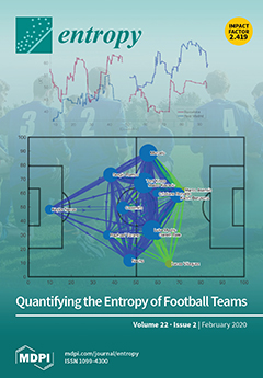
In recent years, analysis of the organization and performance of football teams has undergone a methodological revolution, thanks to emergent technologies recording player activity during a match. Nowadays, it is possible to measure all events occurring on the pitch (passes, interceptions, shots, goals, fouls, etc.) with precise temporal and spatial coordinates. In this paper, we investigated the spatial and temporal entropies of football teams, focusing on the locations of all passes made during a match and the evolution of the organization of the corresponding passing networks. The analysis of football teams as time-evolving networks reveals interesting insights about what network parameters behave more/less randomly and, therefore, could be used as indicators for the prediction of future events. View this paper.
  • Issues are regarded as officially published after their release is announced to the table of contents alert mailing list.
  • You may sign up for e-mail alerts to receive table of contents of newly released issues.
  • PDF is the official format for papers published in both, html and pdf forms. To view the papers in pdf format, click on the "PDF Full-text" link, and use the free Adobe Reader to open them.
Order results
Result details
Section
Select all
Export citation of selected articles as:
23 pages, 3145 KiB  
Article
A Novel Multi-Criteria Decision-Making Model for Building Material Supplier Selection Based on Entropy-AHP Weighted TOPSIS
by Chun-Ho Chen
Entropy 2020, 22(2), 259; https://doi.org/10.3390/e22020259 - 24 Feb 2020
Cited by 209 | Viewed by 12603
Abstract
The type of criterion weight can be distinguished according to different decision methods. Subjective weights are given by decision makers based on their knowledge, experience, expertise, and other factors. Objective weights are obtained through multi-step calculations of the evaluation matrix constructed from the [...] Read more.
The type of criterion weight can be distinguished according to different decision methods. Subjective weights are given by decision makers based on their knowledge, experience, expertise, and other factors. Objective weights are obtained through multi-step calculations of the evaluation matrix constructed from the actual information about the evaluation criteria of the alternatives. A single consideration of these two types of weights often results in biased results. In addition, in order to build an effective supply chain source, buyers must find suitable quality products and/or service providers in the process of supplier selection. Based on the above reasons, it is difficult to accurately select the appropriate alternative. The main contribution of this paper is to combine entropy weight, analytic hierarchy process (AHP) weight, and the technique for order preference by similarity to an ideal solution (TOPSIS) method into a suitable multi-criteria decision making (MCDM) solution. The TOPSIS method is extended with entropy-AHP weights, and entropy-AHP weights are used instead of subjective weights. A novel decision-making model of TOPSIS integrated entropy-AHP weights is proposed to select the appropriate supplier. Finally, we take the selection of building material suppliers as an example and use sensitivity analysis to show that the combination of the TOPSIS method based on entropy-AHP weights can effectively select the appropriate supplier. Full article
Show Figures

Figure 1

Figure 1
<p>Research framework and analytic processes of sections and steps.</p>
Full article ">Figure 2
<p>Schematic diagram of the hierarchy.</p>
Full article ">Figure 3
<p>Hierarchical analysis diagram of this study.</p>
Full article ">Figure 4
<p>Comprehensive proximity of supplier alternatives.</p>
Full article ">Figure 5
<p>Sensitivity analysis of the facet weight to the outcome of the alternatives. ntropy-AHP TOPSIS vs. AHP-based TOPSIS.</p>
Full article ">Figure 5 Cont.
<p>Sensitivity analysis of the facet weight to the outcome of the alternatives. ntropy-AHP TOPSIS vs. AHP-based TOPSIS.</p>
Full article ">
24 pages, 2462 KiB  
Article
Gaussian Process Based Expected Information Gain Computation for Bayesian Optimal Design
by Zhihang Xu and Qifeng Liao
Entropy 2020, 22(2), 258; https://doi.org/10.3390/e22020258 - 24 Feb 2020
Cited by 10 | Viewed by 5241
Abstract
Optimal experimental design (OED) is of great significance in efficient Bayesian inversion. A popular choice of OED methods is based on maximizing the expected information gain (EIG), where expensive likelihood functions are typically involved. To reduce the computational cost, in this work, a [...] Read more.
Optimal experimental design (OED) is of great significance in efficient Bayesian inversion. A popular choice of OED methods is based on maximizing the expected information gain (EIG), where expensive likelihood functions are typically involved. To reduce the computational cost, in this work, a novel double-loop Bayesian Monte Carlo (DLBMC) method is developed to efficiently compute the EIG, and a Bayesian optimization (BO) strategy is proposed to obtain its maximizer only using a small number of samples. For Bayesian Monte Carlo posed on uniform and normal distributions, our analysis provides explicit expressions for the mean estimates and the bounds of their variances. The accuracy and the efficiency of our DLBMC and BO based optimal design are validated and demonstrated with numerical experiments. Full article
(This article belongs to the Section Multidisciplinary Applications)
Show Figures

Figure 1

Figure 1
<p>Estimated expected information gain (EIG) profile over the design space for test problem 1. (<b>a</b>) Pink and gray shaded areas represent the interval containing 80% of 20 independent estimates of two estimators at each <span class="html-italic">d</span> respectively. Blue line and red line indicates the means of estimates. (<b>b</b>) One set of realizations of the two estimators.</p>
Full article ">Figure 2
<p>(<b>Left</b>) Error averaging over <math display="inline"><semantics> <mrow> <mi>n</mi> <mo>=</mo> <mn>20</mn> </mrow> </semantics></math> trails versus the sample size of DLMC and DLBMC. (<b>Right</b>) Sample variance versus the repeat times for different sample sizes of double-loop Monte Carlo (DLMC) and double-loop Bayesian Monte Carlo (DLBMC) (numbers in the parenthesis indicate the sample sizes).</p>
Full article ">Figure 3
<p>Estimated EIG profile over the design space for test problem 2. Pink and gray shaded areas represent the interval containing 80% of 20 independent estimates of EIG at each <span class="html-italic">d</span> for DLBMC and DLMC respectively. Blue line and red line denotes the means of these estimators. Green line denotes the reference solution given by DLMC with <math display="inline"><semantics> <msup> <mn>10</mn> <mn>5</mn> </msup> </semantics></math> samples.</p>
Full article ">Figure 4
<p>Posterior density functions given by different designs.</p>
Full article ">Figure 5
<p>(<b>Left</b>) Maximum EIG value at iteration <span class="html-italic">t</span> of Bayesian optimization. (<b>Right</b>) Average cumulative regret at iteration <span class="html-italic">t</span> of Bayesian optimization. <math display="inline"><semantics> <mrow> <mi>K</mi> <mo>=</mo> <mn>1</mn> </mrow> </semantics></math>, test problem 3.</p>
Full article ">Figure 6
<p>Sensor locations for <math display="inline"><semantics> <mrow> <mi>K</mi> <mo>=</mo> <mn>1</mn> </mrow> </semantics></math>, test problem 3.</p>
Full article ">Figure 7
<p>Value of EIG versus the relative errors averaged over 20 trails, <math display="inline"><semantics> <mrow> <mi>K</mi> <mo>=</mo> <mn>1</mn> </mrow> </semantics></math>, test problem 3.</p>
Full article ">Figure 8
<p>Optimal design (each line connecting blue circle and red circle represents a pair of optimal design points), <math display="inline"><semantics> <mrow> <mi>K</mi> <mo>=</mo> <mn>2</mn> </mrow> </semantics></math>, test problem 3.</p>
Full article ">Figure 9
<p>Value of EIG versus the relative errors averaged over 20 trails, <math display="inline"><semantics> <mrow> <mi>K</mi> <mo>=</mo> <mn>2</mn> </mrow> </semantics></math>, test problem 3.</p>
Full article ">Figure 10
<p>Comparison of the true source field and estimated source fields by MAP and mean estimates for <math display="inline"><semantics> <mrow> <mi>K</mi> <mo>=</mo> <mn>2</mn> </mrow> </semantics></math>, test problem 3.</p>
Full article ">Figure 11
<p>Value of EIG versus the relative errors averaged over 20 trails, <math display="inline"><semantics> <mrow> <mi>K</mi> <mo>=</mo> <mn>3</mn> </mrow> </semantics></math>, test problem 3.</p>
Full article ">Figure 12
<p>Comparison of the true source field and estimated source fields by MAP and mean estimates for <math display="inline"><semantics> <mrow> <mi>K</mi> <mo>=</mo> <mn>3</mn> </mrow> </semantics></math>, test problem 3.</p>
Full article ">Figure 12 Cont.
<p>Comparison of the true source field and estimated source fields by MAP and mean estimates for <math display="inline"><semantics> <mrow> <mi>K</mi> <mo>=</mo> <mn>3</mn> </mrow> </semantics></math>, test problem 3.</p>
Full article ">Figure 13
<p>Histograms of <math display="inline"><semantics> <mrow> <msubsup> <mi>E</mi> <mrow> <mi>MAP</mi> </mrow> <mrow> <mo stretchy="false">(</mo> <mi>random</mi> <mo stretchy="false">)</mo> </mrow> </msubsup> <mo>/</mo> <msubsup> <mi>E</mi> <mrow> <mi>MAP</mi> </mrow> <mrow> <mo stretchy="false">(</mo> <mi>opt</mi> <mo stretchy="false">)</mo> </mrow> </msubsup> </mrow> </semantics></math>. Green lines denotes the kernel smoothing function estimates.</p>
Full article ">
11 pages, 3606 KiB  
Article
Characteristics of Nonthermal Dupree Diffusion on Space-Charge Wave in a Kappa Distribution Plasma Column with Turbulent Diffusion
by Myoung-Jae Lee and Young-Dae Jung
Entropy 2020, 22(2), 257; https://doi.org/10.3390/e22020257 - 24 Feb 2020
Cited by 2 | Viewed by 2463
Abstract
The nonthermal diffusion effects on the dispersion equations of ion-acoustic space-charge wave (SCW) in a nonthermal plasma column composed of nonthermal turbulent electrons and cold ions are investigated based on the analysis of normal modes and the separation of variables. It is found [...] Read more.
The nonthermal diffusion effects on the dispersion equations of ion-acoustic space-charge wave (SCW) in a nonthermal plasma column composed of nonthermal turbulent electrons and cold ions are investigated based on the analysis of normal modes and the separation of variables. It is found that the real portion of the wave frequency of the SCW in a Maxwellian plasma is greater than that in a nonthermal plasma. It is also found that the magnitude of the damping rate of the SCW decreases with an increase of the spectral index of the nonthermal plasma. It is also shown that the magnitude of the scaled damping rate increases with an increase of the Dupree diffusion coefficient. Moreover, the influence of the nonthermal character of the nonthermal plasma on the damping rate is found to be more significant in turbulent plasmas with higher diffusion coefficient. The variations of the wave frequency and the growth rate due to the characteristics of nonthermal diffusion are also discussed. Full article
(This article belongs to the Special Issue Theoretical Aspects of Kappa Distributions)
Show Figures

Figure 1

Figure 1
<p>The scaled real part <math display="inline"><semantics> <mrow> <msub> <mover accent="true"> <mi>ω</mi> <mo stretchy="false">¯</mo> </mover> <mi>R</mi> </msub> </mrow> </semantics></math> of the wave frequency of the space-charge wave (SCW) as a function of the scaled axial wave number <math display="inline"><semantics> <mrow> <msub> <mover accent="true"> <mi>k</mi> <mo stretchy="false">¯</mo> </mover> <mo>∥</mo> </msub> </mrow> </semantics></math> for <math display="inline"><semantics> <mrow> <mover accent="true"> <mi>R</mi> <mo stretchy="false">¯</mo> </mover> <mo>=</mo> <mn>3</mn> </mrow> </semantics></math> and the first-harmonic, i.e., <math display="inline"><semantics> <mrow> <msub> <mi>α</mi> <mrow> <mn>01</mn> </mrow> </msub> <mo>=</mo> <mn>2</mn> <mrow> <mo>.</mo> <mn>4048</mn> </mrow> </mrow> </semantics></math>. The solid line is the case of <math display="inline"><semantics> <mrow> <mi>κ</mi> <mo>=</mo> <mn>2</mn> </mrow> </semantics></math>. The dashed line is the case of <math display="inline"><semantics> <mrow> <mi>κ</mi> <mo>=</mo> <mn>3</mn> </mrow> </semantics></math>. The dotted line is the case of <math display="inline"><semantics> <mrow> <mi>κ</mi> <mo>=</mo> <mn>5</mn> </mrow> </semantics></math>. The dash-dot is the case of <math display="inline"><semantics> <mrow> <mi>κ</mi> <mo>→</mo> <mo>∞</mo> </mrow> </semantics></math>, i.e., Maxwellian case.</p>
Full article ">Figure 2
<p>The scaled real part <math display="inline"><semantics> <mrow> <msub> <mover accent="true"> <mi>ω</mi> <mo stretchy="false">¯</mo> </mover> <mi>R</mi> </msub> </mrow> </semantics></math> of the wave frequency of the SCW as a function of the scaled axial wave number <math display="inline"><semantics> <mrow> <msub> <mover accent="true"> <mi>k</mi> <mo stretchy="false">¯</mo> </mover> <mo>∥</mo> </msub> </mrow> </semantics></math> for <math display="inline"><semantics> <mrow> <mover accent="true"> <mi>R</mi> <mo stretchy="false">¯</mo> </mover> <mo>=</mo> <mn>5</mn> </mrow> </semantics></math>. The solid line is the case of <math display="inline"><semantics> <mrow> <mi>κ</mi> <mo>=</mo> <mn>2</mn> </mrow> </semantics></math> and the first-harmonic, i.e., <math display="inline"><semantics> <mrow> <msub> <mi>α</mi> <mrow> <mn>01</mn> </mrow> </msub> <mo>=</mo> <mn>2</mn> <mrow> <mo>.</mo> <mn>4048</mn> </mrow> </mrow> </semantics></math>. The dashed line is the case of <math display="inline"><semantics> <mrow> <mi>κ</mi> <mo>=</mo> <mn>2</mn> </mrow> </semantics></math> and the second-harmonic, i.e., <math display="inline"><semantics> <mrow> <msub> <mi>α</mi> <mrow> <mn>02</mn> </mrow> </msub> <mo>=</mo> <mn>5</mn> <mrow> <mo>.</mo> <mn>5201</mn> </mrow> </mrow> </semantics></math>. The dotted line is the case of <math display="inline"><semantics> <mrow> <mi>κ</mi> <mo>=</mo> <mn>4</mn> </mrow> </semantics></math> and the first-harmonic, i.e., <math display="inline"><semantics> <mrow> <msub> <mi>α</mi> <mrow> <mn>01</mn> </mrow> </msub> <mo>=</mo> <mn>2</mn> <mrow> <mo>.</mo> <mn>4048</mn> </mrow> </mrow> </semantics></math>. The dash-dot is the case of <math display="inline"><semantics> <mrow> <mi>κ</mi> <mo>=</mo> <mn>4</mn> </mrow> </semantics></math> and the second-harmonic, i.e., <math display="inline"><semantics> <mrow> <msub> <mi>α</mi> <mrow> <mn>02</mn> </mrow> </msub> <mo>=</mo> <mn>5</mn> <mrow> <mo>.</mo> <mn>5201</mn> </mrow> </mrow> </semantics></math>.</p>
Full article ">Figure 3
<p>(<b>a</b>) Surface plot; (<b>b</b>) Contour plot of the scaled real part <math display="inline"><semantics> <mrow> <msub> <mover accent="true"> <mi>ω</mi> <mo stretchy="false">¯</mo> </mover> <mi>R</mi> </msub> </mrow> </semantics></math> of the wave frequency of the SCW as a function of the spectral index <math display="inline"><semantics> <mi>κ</mi> </semantics></math> and the scaled radius <math display="inline"><semantics> <mover accent="true"> <mi>R</mi> <mo stretchy="false">¯</mo> </mover> </semantics></math> of the cylindrical plasma column for <math display="inline"><semantics> <mrow> <msub> <mover accent="true"> <mi>k</mi> <mo stretchy="false">¯</mo> </mover> <mo>∥</mo> </msub> <mo>=</mo> <mn>5</mn> </mrow> </semantics></math> and the first-harmonic, i.e., <math display="inline"><semantics> <mrow> <msub> <mi>α</mi> <mrow> <mn>01</mn> </mrow> </msub> <mo>=</mo> <mn>2</mn> <mrow> <mo>.</mo> <mn>4048</mn> </mrow> </mrow> </semantics></math>.</p>
Full article ">Figure 4
<p>The scaled imaginary part of the wave frequency, i.e., the scaled damping rate <math display="inline"><semantics> <mover accent="true"> <mi>γ</mi> <mo stretchy="false">¯</mo> </mover> </semantics></math>, as a function of the scaled axial wave number <math display="inline"><semantics> <mrow> <msub> <mover accent="true"> <mi>k</mi> <mo stretchy="false">¯</mo> </mover> <mo>∥</mo> </msub> </mrow> </semantics></math> for <math display="inline"><semantics> <mrow> <mover accent="true"> <mi>D</mi> <mo stretchy="false">¯</mo> </mover> <mo>=</mo> <mn>1</mn> </mrow> </semantics></math>; <math display="inline"><semantics> <mrow> <mover accent="true"> <mi>R</mi> <mo stretchy="false">¯</mo> </mover> <mo>=</mo> <mn>3</mn> </mrow> </semantics></math>; and the first-harmonic, i.e., <math display="inline"><semantics> <mrow> <msub> <mi>α</mi> <mrow> <mn>01</mn> </mrow> </msub> <mo>=</mo> <mn>2</mn> <mrow> <mo>.</mo> <mn>4048</mn> </mrow> </mrow> </semantics></math>. The solid line is the case of <math display="inline"><semantics> <mrow> <mi>κ</mi> <mo>=</mo> <mn>2</mn> </mrow> </semantics></math>. The dashed line is the case of <math display="inline"><semantics> <mrow> <mi>κ</mi> <mo>=</mo> <mn>3</mn> </mrow> </semantics></math>. The dotted line is the case of <math display="inline"><semantics> <mrow> <mi>κ</mi> <mo>=</mo> <mn>5</mn> </mrow> </semantics></math>. The dash-dot is the case of <math display="inline"><semantics> <mrow> <mi>κ</mi> <mo>→</mo> <mo>∞</mo> </mrow> </semantics></math>, i.e., Maxwellian case.</p>
Full article ">Figure 5
<p>The scaled damping rate <math display="inline"><semantics> <mover accent="true"> <mi>γ</mi> <mo stretchy="false">¯</mo> </mover> </semantics></math> of the SCW as a function of the scaled axial wave number <math display="inline"><semantics> <mrow> <msub> <mover accent="true"> <mi>k</mi> <mo stretchy="false">¯</mo> </mover> <mo>∥</mo> </msub> </mrow> </semantics></math> for <math display="inline"><semantics> <mrow> <mi>κ</mi> <mo>=</mo> <mn>2</mn> </mrow> </semantics></math> and <math display="inline"><semantics> <mrow> <mover accent="true"> <mi>R</mi> <mo stretchy="false">¯</mo> </mover> <mo>=</mo> <mn>5</mn> </mrow> </semantics></math>. The solid line is the case of <math display="inline"><semantics> <mrow> <mover accent="true"> <mi>D</mi> <mo stretchy="false">¯</mo> </mover> <mo>=</mo> <mn>1</mn> </mrow> </semantics></math> and the first-harmonic, i.e., <math display="inline"><semantics> <mrow> <msub> <mi>α</mi> <mrow> <mn>01</mn> </mrow> </msub> <mo>=</mo> <mn>2</mn> <mrow> <mo>.</mo> <mn>4048</mn> </mrow> </mrow> </semantics></math>. The dashed line is the case of <math display="inline"><semantics> <mrow> <mover accent="true"> <mi>D</mi> <mo stretchy="false">¯</mo> </mover> <mo>=</mo> <mn>1</mn> </mrow> </semantics></math> and the second-harmonic, i.e., <math display="inline"><semantics> <mrow> <msub> <mi>α</mi> <mrow> <mn>02</mn> </mrow> </msub> <mo>=</mo> <mn>5</mn> <mrow> <mo>.</mo> <mn>5201</mn> </mrow> </mrow> </semantics></math>. The dotted line is the case of <math display="inline"><semantics> <mrow> <mover accent="true"> <mi>D</mi> <mo stretchy="false">¯</mo> </mover> <mo>=</mo> <mn>3</mn> </mrow> </semantics></math> and the first-harmonic, i.e., <math display="inline"><semantics> <mrow> <msub> <mi>α</mi> <mrow> <mn>01</mn> </mrow> </msub> <mo>=</mo> <mn>2</mn> <mrow> <mo>.</mo> <mn>4048</mn> </mrow> </mrow> </semantics></math>. The dash-dot is the case of <math display="inline"><semantics> <mrow> <mover accent="true"> <mi>D</mi> <mo stretchy="false">¯</mo> </mover> <mo>=</mo> <mn>3</mn> </mrow> </semantics></math> and the second-harmonic, i.e., <math display="inline"><semantics> <mrow> <msub> <mi>α</mi> <mrow> <mn>02</mn> </mrow> </msub> <mo>=</mo> <mn>5</mn> <mrow> <mo>.</mo> <mn>5201</mn> </mrow> </mrow> </semantics></math>.</p>
Full article ">Figure 6
<p>(<b>a</b>) Surface plot; (<b>b</b>) Contour plot of the scaled damping rate <math display="inline"><semantics> <mover accent="true"> <mi>γ</mi> <mo stretchy="false">¯</mo> </mover> </semantics></math> of the SCW as a function of the scaled radius <math display="inline"><semantics> <mover accent="true"> <mi>R</mi> <mo stretchy="false">¯</mo> </mover> </semantics></math> of the cylindrical plasma column and the spectral index <math display="inline"><semantics> <mi>κ</mi> </semantics></math> for <math display="inline"><semantics> <mrow> <msub> <mover accent="true"> <mi>k</mi> <mo stretchy="false">¯</mo> </mover> <mo>∥</mo> </msub> <mo>=</mo> <mn>1</mn> </mrow> </semantics></math> and <math display="inline"><semantics> <mrow> <mover accent="true"> <mi>D</mi> <mo stretchy="false">¯</mo> </mover> <mo>=</mo> <mn>1</mn> </mrow> </semantics></math>.</p>
Full article ">Figure 7
<p>(<b>a</b>) Surface plot; (<b>b</b>) Contour plot of the scaled damping rate <math display="inline"><semantics> <mover accent="true"> <mi>γ</mi> <mo stretchy="false">¯</mo> </mover> </semantics></math> of the SCW as a function of the scaled diffusion coefficient <math display="inline"><semantics> <mover accent="true"> <mi>D</mi> <mo stretchy="false">¯</mo> </mover> </semantics></math> and the spectral index <math display="inline"><semantics> <mi>κ</mi> </semantics></math> for <math display="inline"><semantics> <mrow> <msub> <mover accent="true"> <mi>k</mi> <mo stretchy="false">¯</mo> </mover> <mo>∥</mo> </msub> <mo>=</mo> <mn>1</mn> </mrow> </semantics></math> and <math display="inline"><semantics> <mrow> <mover accent="true"> <mi>R</mi> <mo stretchy="false">¯</mo> </mover> <mo>=</mo> <mn>5</mn> </mrow> </semantics></math>.</p>
Full article ">
14 pages, 496 KiB  
Article
Phylogenetic Analysis of HIV-1 Genomes Based on the Position-Weighted K-mers Method
by Yuanlin Ma, Zuguo Yu, Runbin Tang, Xianhua Xie, Guosheng Han and Vo V. Anh
Entropy 2020, 22(2), 255; https://doi.org/10.3390/e22020255 - 23 Feb 2020
Cited by 14 | Viewed by 3741
Abstract
HIV-1 viruses, which are predominant in the family of HIV viruses, have strong pathogenicity and infectivity. They can evolve into many different variants in a very short time. In this study, we propose a new and effective alignment-free method for the phylogenetic analysis [...] Read more.
HIV-1 viruses, which are predominant in the family of HIV viruses, have strong pathogenicity and infectivity. They can evolve into many different variants in a very short time. In this study, we propose a new and effective alignment-free method for the phylogenetic analysis of HIV-1 viruses using complete genome sequences. Our method combines the position distribution information and the counts of the k-mers together. We also propose a metric to determine the optimal k value. We name our method the Position-Weighted k-mers (PWkmer) method. Validation and comparison with the Robinson–Foulds distance method and the modified bootstrap method on a benchmark dataset show that our method is reliable for the phylogenetic analysis of HIV-1 viruses. PWkmer can resolve within-group variations for different known subtypes of Group M of HIV-1 viruses. This method is simple and computationally fast for whole genome phylogenetic analysis. Full article
(This article belongs to the Special Issue Statistical Inference from High Dimensional Data)
Show Figures

Figure 1

Figure 1
<p>The trend chart of <span class="html-italic">k</span> value vs. scoring scheme <span class="html-italic">score(k)</span>. The red circles represent the score of the HIV dataset for different <span class="html-italic">k</span> values, and the blue dots represent the score of the HEV dataset for different <span class="html-italic">k</span> value.</p>
Full article ">Figure 2
<p>Subtyping of HIV based on position weighted <span class="html-italic">k</span>-mers feature for whole genome sequences. The Neighbor-Joining (NJ) tree of 44 HIV whole genomes is constructed by position weighted <span class="html-italic">k</span>-mers feature distance matrix <math display="inline"><semantics> <mrow> <mo>(</mo> <mi>k</mi> <mo>=</mo> <mn>8</mn> <mo>)</mo> </mrow> </semantics></math>.</p>
Full article ">Figure 3
<p>Subtyping of HIV based on alignment for whole genome sequences. The NJ tree of 44 HIV whole genomes is constructed by ClustalX.</p>
Full article ">Figure 4
<p>Robinson–Foulds distance between phylogenetic trees reconstructed by the <span class="html-italic">PWkmer</span> method, the CVTree method [<a href="#B20-entropy-22-00255" class="html-bibr">20</a>], the DLTree [<a href="#B12-entropy-22-00255" class="html-bibr">12</a>] method, and the tree reconstructed by ClustalX method for 44 HIV genome sequence in <a href="#entropy-22-00255-t001" class="html-table">Table 1</a> (we selected their optimal result tree by CVTree and DLTree).</p>
Full article ">Figure 5
<p>The modified bootstrap consensus tree for <a href="#entropy-22-00255-f002" class="html-fig">Figure 2</a> based on 100 replicates.</p>
Full article ">
19 pages, 1671 KiB  
Review
Entropy Generation Methodology for Defect Analysis of Electronic and Mechanical Components—A Review
by Miao Cai, Peng Cui, Yikang Qin, Daoshuang Geng, Qiqin Wei, Xiyou Wang, Daoguo Yang and Guoqi Zhang
Entropy 2020, 22(2), 254; https://doi.org/10.3390/e22020254 - 23 Feb 2020
Cited by 12 | Viewed by 6299
Abstract
Understanding the defect characterization of electronic and mechanical components is a crucial step in diagnosing component lifetime. Technologies for determining reliability, such as thermal modeling, cohesion modeling, statistical distribution, and entropy generation analysis, have been developed widely. Defect analysis based on the irreversibility [...] Read more.
Understanding the defect characterization of electronic and mechanical components is a crucial step in diagnosing component lifetime. Technologies for determining reliability, such as thermal modeling, cohesion modeling, statistical distribution, and entropy generation analysis, have been developed widely. Defect analysis based on the irreversibility entropy generation methodology is favorable for electronic and mechanical components because the second law of thermodynamics plays a unique role in the analysis of various damage assessment problems encountered in the engineering field. In recent years, numerical and theoretical studies involving entropy generation methodologies have been carried out to predict and diagnose the lifetime of electronic and mechanical components. This work aimed to review previous defect analysis studies that used entropy generation methodologies for electronic and mechanical components. The methodologies are classified into two categories, namely, damage analysis for electronic devices and defect diagnosis for mechanical components. Entropy generation formulations are also divided into two detailed derivations and are summarized and discussed by combining their applications. This work is expected to clarify the relationship among entropy generation methodologies, and benefit the research and development of reliable engineering components. Full article
(This article belongs to the Section Entropy Reviews)
Show Figures

Figure 1

Figure 1
<p>Application of entropy generation in the reliability field. (Capacitor [<a href="#B12-entropy-22-00254" class="html-bibr">12</a>], resistor [<a href="#B11-entropy-22-00254" class="html-bibr">11</a>], light emitting diode (LED) [<a href="#B13-entropy-22-00254" class="html-bibr">13</a>], pyroelectric sensor [<a href="#B30-entropy-22-00254" class="html-bibr">30</a>], through silicon via [<a href="#B15-entropy-22-00254" class="html-bibr">15</a>], solder ball [<a href="#B9-entropy-22-00254" class="html-bibr">9</a>], 304 stainless steel [<a href="#B18-entropy-22-00254" class="html-bibr">18</a>], aluminum block [<a href="#B7-entropy-22-00254" class="html-bibr">7</a>], sink [<a href="#B25-entropy-22-00254" class="html-bibr">25</a>], fin [<a href="#B31-entropy-22-00254" class="html-bibr">31</a>], circuit board [<a href="#B22-entropy-22-00254" class="html-bibr">22</a>], and heat exchanger).</p>
Full article ">Figure 2
<p>Entropy generation analysis for damage characterization of electronic systems (microscopic defect from [<a href="#B14-entropy-22-00254" class="html-bibr">14</a>]).</p>
Full article ">Figure 3
<p>Schematic of monitoring entropy generation rate of capacitor (<b>a</b>) [<a href="#B12-entropy-22-00254" class="html-bibr">12</a>] and resistor (<b>b</b>) [<a href="#B11-entropy-22-00254" class="html-bibr">11</a>].</p>
Full article ">Figure 4
<p>Schematic of exergy diffusion of flip-chip package model.</p>
Full article ">Figure 5
<p>FFE (fracture fatigue entropy) of AISI 1018 carbon steel [<a href="#B64-entropy-22-00254" class="html-bibr">64</a>].</p>
Full article ">
10 pages, 757 KiB  
Article
(1,0)-Super Solutions of (k,s)-CNF Formula
by Zufeng Fu, Daoyun Xu and Yongping Wang
Entropy 2020, 22(2), 253; https://doi.org/10.3390/e22020253 - 23 Feb 2020
Cited by 3 | Viewed by 3022
Abstract
A (1,0)-super solution is a satisfying assignment such that if the value of any one variable is flipped to the opposite value, the new assignment is still a satisfying assignment. Namely, every clause must contain at least two satisfied literals. Because of its [...] Read more.
A (1,0)-super solution is a satisfying assignment such that if the value of any one variable is flipped to the opposite value, the new assignment is still a satisfying assignment. Namely, every clause must contain at least two satisfied literals. Because of its robustness, super solutions are concerned in combinatorial optimization problems and decision problems. In this paper, we investigate the existence conditions of the (1,0)-super solution of ( k , s ) -CNF formula, and give a reduction method that transform from k-SAT to (1,0)- ( k + 1 , s ) -SAT if there is a ( k + 1 , s )-CNF formula without a (1,0)-super solution. Here, ( k , s ) -CNF is a subclass of CNF in which each clause has exactly k distinct literals, and each variable occurs at most s times. (1,0)- ( k , s ) -SAT is a problem to decide whether a ( k , s ) -CNF formula has a (1,0)-super solution. We prove that for k > 3 , if there exists a ( k , s ) -CNF formula without a (1,0)-super solution, (1,0)- ( k , s ) -SAT is NP-complete. We show that for k > 3 , there is a critical function φ ( k ) such that every ( k , s ) -CNF formula has a (1,0)-super solution for s φ ( k ) and (1,0)- ( k , s ) -SAT is NP-complete for s > φ ( k ) . We further show some properties of the critical function φ ( k ) . Full article
(This article belongs to the Section Information Theory, Probability and Statistics)
19 pages, 2411 KiB  
Article
Semi-Supervised Bidirectional Long Short-Term Memory and Conditional Random Fields Model for Named-Entity Recognition Using Embeddings from Language Models Representations
by Min Zhang, Guohua Geng and Jing Chen
Entropy 2020, 22(2), 252; https://doi.org/10.3390/e22020252 - 22 Feb 2020
Cited by 22 | Viewed by 5377
Abstract
Increasingly, popular online museums have significantly changed the way people acquire cultural knowledge. These online museums have been generating abundant amounts of cultural relics data. In recent years, researchers have used deep learning models that can automatically extract complex features and have rich [...] Read more.
Increasingly, popular online museums have significantly changed the way people acquire cultural knowledge. These online museums have been generating abundant amounts of cultural relics data. In recent years, researchers have used deep learning models that can automatically extract complex features and have rich representation capabilities to implement named-entity recognition (NER). However, the lack of labeled data in the field of cultural relics makes it difficult for deep learning models that rely on labeled data to achieve excellent performance. To address this problem, this paper proposes a semi-supervised deep learning model named SCRNER (Semi-supervised model for Cultural Relics’ Named Entity Recognition) that utilizes the bidirectional long short-term memory (BiLSTM) and conditional random fields (CRF) model trained by seldom labeled data and abundant unlabeled data to attain an effective performance. To satisfy the semi-supervised sample selection, we propose a repeat-labeled (relabeled) strategy to select samples of high confidence to enlarge the training set iteratively. In addition, we use embeddings from language model (ELMo) representations to dynamically acquire word representations as the input of the model to solve the problem of the blurred boundaries of cultural objects and Chinese characteristics of texts in the field of cultural relics. Experimental results demonstrate that our proposed model, trained on limited labeled data, achieves an effective performance in the task of named entity recognition of cultural relics. Full article
(This article belongs to the Special Issue Information Theory and Graph Signal Processing)
Show Figures

Figure 1

Figure 1
<p>Overview of the semi-supervised bidirectional long short-term memory (BiLSTM)-conditional random fields (CRF) framework for named-entity recognition (NER).</p>
Full article ">Figure 2
<p>Embedding from Language Model.</p>
Full article ">Figure 3
<p>The architecture of embeddings from language models (ELMO)-based BiLSTM-CRF model.</p>
Full article ">Figure 4
<p>Architecture of the LSTM memory.</p>
Full article ">Figure 5
<p>Performance comparison of the percentage of initial labeled data. (<b>a</b>) Accuracy curves; (<b>b</b>) <span class="html-italic">F</span><sub>1</sub>-score curves.</p>
Full article ">Figure 6
<p>Performance comparison of SCNER and word embeddings. Note: Word, the model that uses word embedding as Word representation; Character, the model that uses character embedding as the word representation; W_C, the model that combines word and character embedding; SCRNER, the model proposed in this study. (<b>a</b>) Accuracy curves; (<b>b</b>) <span class="html-italic">F</span><sub>1</sub>-score curves.</p>
Full article ">Figure 7
<p>Performance Comparison of BiLSTM-CRF and SCRNER in four entities. Note: BiLSTM_CRF is the framework proposed by Yang H et al. [<a href="#B11-entropy-22-00252" class="html-bibr">11</a>].</p>
Full article ">
14 pages, 5353 KiB  
Article
Self-Propulsion Enhances Polymerization
by Maximino Aldana, Miguel Fuentes-Cabrera and Martín Zumaya
Entropy 2020, 22(2), 251; https://doi.org/10.3390/e22020251 - 22 Feb 2020
Cited by 3 | Viewed by 3693
Abstract
Self-assembly is a spontaneous process through which macroscopic structures are formed from basic microscopic constituents (e.g., molecules or colloids). By contrast, the formation of large biological molecules inside the cell (such as proteins or nucleic acids) is a process more akin to self-organization [...] Read more.
Self-assembly is a spontaneous process through which macroscopic structures are formed from basic microscopic constituents (e.g., molecules or colloids). By contrast, the formation of large biological molecules inside the cell (such as proteins or nucleic acids) is a process more akin to self-organization than to self-assembly, as it requires a constant supply of external energy. Recent studies have tried to merge self-assembly with self-organization by analyzing the assembly of self-propelled (or active) colloid-like particles whose motion is driven by a permanent source of energy. Here we present evidence that points to the fact that self-propulsion considerably enhances the assembly of polymers: self-propelled molecules are found to assemble faster into polymer-like structures than non self-propelled ones. The average polymer length increases towards a maximum as the self-propulsion force increases. Beyond this maximum, the average polymer length decreases due to the competition between bonding energy and disruptive forces that result from collisions. The assembly of active molecules might have promoted the formation of large pre-biotic polymers that could be the precursors of the informational polymers we observe nowadays. Full article
(This article belongs to the Special Issue Thermodynamics and Entropy for Self-Assembly and Self-Organization)
Show Figures

Figure 1

Figure 1
<p>(<b>a</b>) Schematic representation of the basic rigid molecule. The sides of the molecule are discretized into spherical subunits with positions <math display="inline"><semantics> <msubsup> <mi mathvariant="bold">e</mi> <mi>i</mi> <mi>α</mi> </msubsup> </semantics></math> which exert attractive or repulsive forces on the spherical subunits of other molecules. The entire molecule is characterized by the position <math display="inline"><semantics> <msub> <mi mathvariant="bold">r</mi> <mi>i</mi> </msub> </semantics></math> of the center of mass, its velocity <math display="inline"><semantics> <msub> <mi mathvariant="bold">v</mi> <mi>i</mi> </msub> </semantics></math> and orientation <math display="inline"><semantics> <msub> <mover accent="true"> <mi mathvariant="bold">u</mi> <mo>^</mo> </mover> <mi>i</mi> </msub> </semantics></math>. Note that the velocity and orientation are not necessarily parallel. The self-propulsion force always acts in the direction of the orientation vector <math display="inline"><semantics> <msub> <mover accent="true"> <mi mathvariant="bold">u</mi> <mo>^</mo> </mover> <mi>i</mi> </msub> </semantics></math>. The edges of the molecule are colored according to the repulsive or attractive forces they exert on other molecules: if two molecules collide through edges of the same color, the force is repulsive as in (<b>b</b>), whereas the force is attractive only between the green and red edges, as in (<b>c</b>). The dynamics take place on a 2D-space.</p>
Full article ">Figure 2
<p>Snapshots of the system with fully periodic boundary conditions (the <span class="html-italic">bulk</span>) showing the effect of self-propulsion on the assembly of molecules. Different snapshots correspond to different values of the self-propulsion force: (<b>a</b>) <math display="inline"><semantics> <msub> <mi>F</mi> <mrow> <mi>sp</mi> <mo>=</mo> <mn>0</mn> </mrow> </msub> </semantics></math>, (<b>b</b>) <math display="inline"><semantics> <msub> <mi>F</mi> <mrow> <mi>sp</mi> <mo>=</mo> <mn>2.5</mn> </mrow> </msub> </semantics></math>, (<b>c</b>) <math display="inline"><semantics> <msub> <mi>F</mi> <mrow> <mi>sp</mi> <mo>=</mo> <mn>10</mn> </mrow> </msub> </semantics></math>, and (<b>d</b>) <math display="inline"><semantics> <msub> <mi>F</mi> <mrow> <mi>sp</mi> <mo>=</mo> <mn>15</mn> </mrow> </msub> </semantics></math>. In all cases the temperature is <math display="inline"><semantics> <mrow> <mi>T</mi> <mo>=</mo> <mn>0.1</mn> </mrow> </semantics></math> and the number of particles is <math display="inline"><semantics> <mrow> <mi>N</mi> <mo>=</mo> <mn>512</mn> </mrow> </semantics></math>. Note that with no self-propulsion (panel (<b>a</b>), <math display="inline"><semantics> <mrow> <msub> <mi>F</mi> <mi>sp</mi> </msub> <mo>=</mo> <mn>0</mn> </mrow> </semantics></math>), only very small chains are formed. This case would correspond to spontaneous self-assembly. As the self-propulsion force <math display="inline"><semantics> <msub> <mi>F</mi> <mi>sp</mi> </msub> </semantics></math> increases, (panels (<b>b</b>–<b>d</b>)), longer chains appear. It is apparent that self-propulsion considerably improves the assembly of molecules as compared to spontaneous self-assembly. The color gradient represents the length of the chain. All the monomers (<math display="inline"><semantics> <mrow> <mi>L</mi> <mo>=</mo> <mn>1</mn> </mrow> </semantics></math>) are colored in gray.</p>
Full article ">Figure 3
<p>Effect of self-propulsion on the assembly of molecules within semi-periodic boundary conditions (the <span class="html-italic">channel</span>), where the longest sides are rigid boundaries and the shorter ones are periodic. All the snapshots correspond to temperature <math display="inline"><semantics> <mrow> <mi>T</mi> <mo>=</mo> <mn>0.1</mn> </mrow> </semantics></math>, channel aspect ratio <math display="inline"><semantics> <mrow> <mi>R</mi> <mo>=</mo> <msub> <mi>l</mi> <mn>1</mn> </msub> <mo>/</mo> <msub> <mi>l</mi> <mn>2</mn> </msub> <mo>=</mo> <mn>0.25</mn> </mrow> </semantics></math> and <math display="inline"><semantics> <mrow> <mi>N</mi> <mo>=</mo> <mn>512</mn> </mrow> </semantics></math> particles. (<b>a</b>) For <math display="inline"><semantics> <mrow> <msub> <mi>F</mi> <mi>sp</mi> </msub> <mo>=</mo> <mn>0</mn> </mrow> </semantics></math>, i.e., when the motion of the molecules is driven just by thermal noise, only small polymers are formed. The next three panels correspond to non-zero values of the self-propulsion force: (<b>b</b>) <math display="inline"><semantics> <mrow> <msub> <mi>F</mi> <mi>sp</mi> </msub> <mo>=</mo> <mn>5</mn> </mrow> </semantics></math>, (<b>c</b>) <math display="inline"><semantics> <mrow> <msub> <mi>F</mi> <mi>sp</mi> </msub> <mo>=</mo> <mn>7.5</mn> </mrow> </semantics></math>, and (<b>d</b>) <math display="inline"><semantics> <mrow> <msub> <mi>F</mi> <mi>sp</mi> </msub> <mo>=</mo> <mn>10</mn> </mrow> </semantics></math>. Note that as the value of <math display="inline"><semantics> <msub> <mi>F</mi> <mi>sp</mi> </msub> </semantics></math> increases the length of the assembled polymers also increases. Note also that in this case the polymers aggregate in the repulsive boundaries, allowing them to form even longer chains. The color gradient represents the length of the chain. All the monomers (<math display="inline"><semantics> <mrow> <mi>L</mi> <mo>=</mo> <mn>1</mn> </mrow> </semantics></math>) are colored in gray.</p>
Full article ">Figure 4
<p>Average length <math display="inline"><semantics> <mrow> <mo>〈</mo> <mi>L</mi> <mo>〉</mo> </mrow> </semantics></math> of polymer chains as a function of time <span class="html-italic">t</span> for different values of the aspect ratio <span class="html-italic">R</span>, temperature <span class="html-italic">T</span> and self-propulsion force <math display="inline"><semantics> <msub> <mi>F</mi> <mi>sp</mi> </msub> </semantics></math>. Panels (<b>a</b>–<b>c</b>) correspond to temperature <math display="inline"><semantics> <mrow> <mi>T</mi> <mo>=</mo> <mn>0.1</mn> </mrow> </semantics></math> and panels (<b>d</b>–<b>f</b>) to <math display="inline"><semantics> <mrow> <mi>T</mi> <mo>=</mo> <mn>0.25</mn> </mrow> </semantics></math>. Panels (a,d) show the evolution of <math display="inline"><semantics> <mrow> <mo>〈</mo> <mi>L</mi> <mo>(</mo> <mi>t</mi> <mo>)</mo> <mo>〉</mo> </mrow> </semantics></math> in the case of periodic boundary conditions, whereas the remaining panels correspond to the channel geometry for different aspect ratios: in (<b>b</b>,<b>e</b>) <math display="inline"><semantics> <mrow> <mi>R</mi> <mo>=</mo> <mn>0.75</mn> </mrow> </semantics></math> and in (<b>c</b>,<b>f</b>) <math display="inline"><semantics> <mrow> <mi>R</mi> <mo>=</mo> <mn>0.25</mn> </mrow> </semantics></math>. It can be observed that during the computing time <math display="inline"><semantics> <mrow> <mo>〈</mo> <mi>L</mi> <mo>〉</mo> </mrow> </semantics></math> does not reach a stationary value. However, it is evident in all cases that increasing the self-propulsion force <math display="inline"><semantics> <msub> <mi>F</mi> <mi>sp</mi> </msub> </semantics></math> speeds up the formation of polymers. The maximum computing time <math display="inline"><semantics> <mrow> <mi>t</mi> <mo>=</mo> <mn>10</mn> <mo>,</mo> <mn>000</mn> </mrow> </semantics></math> corresponds to <math display="inline"><semantics> <msup> <mn>10</mn> <mn>7</mn> </msup> </semantics></math> time steps in the molecular dynamics simulation. For each curve, the ensemble average <math display="inline"><semantics> <mrow> <mo>〈</mo> <mi>L</mi> <mo>〉</mo> </mrow> </semantics></math> was computed over 20 different realizations.</p>
Full article ">Figure 5
<p>Results for the system with periodic boundary conditions. (<b>a</b>) Probability <math display="inline"><semantics> <mrow> <mi>P</mi> <mo>(</mo> <mi>L</mi> <mo>)</mo> </mrow> </semantics></math> that a polymer of length <span class="html-italic">L</span> is created after <math display="inline"><semantics> <msup> <mn>10</mn> <mn>7</mn> </msup> </semantics></math> time steps. Different colors correspond to different values of the self-propulsion force <math display="inline"><semantics> <msub> <mi>F</mi> <mi>sp</mi> </msub> </semantics></math>. All the simulations in this panel were computed at constant temperature <math display="inline"><semantics> <mrow> <mi>T</mi> <mo>=</mo> <mn>0.1</mn> </mrow> </semantics></math>. The inset shows a magnification of the tail of the distribution <math display="inline"><semantics> <mrow> <mi>P</mi> <mo>(</mo> <mi>L</mi> <mo>)</mo> </mrow> </semantics></math> in order to better appreciate the existence of long polymers. (<b>b</b>) Average chain length <math display="inline"><semantics> <mrow> <mo>〈</mo> <mi>L</mi> <mo>〉</mo> </mrow> </semantics></math> as a function of the self-propelled force <math display="inline"><semantics> <msub> <mi>F</mi> <mi>sp</mi> </msub> </semantics></math> for different values of the temperature <span class="html-italic">T</span>. Note that for lower temperatures, there is an optimal value of <math display="inline"><semantics> <msubsup> <mi>F</mi> <mi>sp</mi> <mo>⋆</mo> </msubsup> </semantics></math> of the self-propulsion force at which <math display="inline"><semantics> <mrow> <mo>〈</mo> <mi>L</mi> <mo>〉</mo> </mrow> </semantics></math> exhibits a maximum. This value is plotted in panel (<b>c</b>) as a function of the temperature <span class="html-italic">T</span>. (<b>d</b>) Temporal evolution of the average polymer length, <math display="inline"><semantics> <mrow> <mo>〈</mo> <mi>L</mi> <mo>(</mo> <mi>t</mi> <mo>)</mo> <mo>〉</mo> </mrow> </semantics></math>, in the high-temperature regime for different values of <math display="inline"><semantics> <msub> <mi>F</mi> <mi>sp</mi> </msub> </semantics></math>. Note that in this case <math display="inline"><semantics> <mrow> <mo>〈</mo> <mi>L</mi> <mo>(</mo> <mi>t</mi> <mo>)</mo> <mo>〉</mo> </mrow> </semantics></math> does reach a stationary value which increases with <math display="inline"><semantics> <msub> <mi>F</mi> <mi>sp</mi> </msub> </semantics></math>. The inset shows the fraction of monomers (<math display="inline"><semantics> <mrow> <mi>L</mi> <mo>=</mo> <mn>1</mn> </mrow> </semantics></math>) and dimers <math display="inline"><semantics> <mrow> <mo>(</mo> <mi>L</mi> <mo>=</mo> <mn>2</mn> <mo>)</mo> </mrow> </semantics></math> in the system in this regime. (Polymers with <math display="inline"><semantics> <mrow> <mi>L</mi> <mo>&gt;</mo> <mn>2</mn> </mrow> </semantics></math> appear in such low quantities that cannot be appreciated on the histogram).</p>
Full article ">Figure 6
<p>Results for the channel with semi-periodic boundary conditions. All the results presented in this figure were computed at constant temperature <math display="inline"><semantics> <mrow> <mi>T</mi> <mo>=</mo> <mn>0.1</mn> </mrow> </semantics></math>. (<b>a</b>) Probability <math display="inline"><semantics> <mrow> <mi>P</mi> <mo>(</mo> <mi>L</mi> <mo>)</mo> </mrow> </semantics></math> that a chain of length <span class="html-italic">L</span> is formed after <math display="inline"><semantics> <msup> <mn>10</mn> <mn>7</mn> </msup> </semantics></math> time steps, for different values of the self-propulsion force <math display="inline"><semantics> <msub> <mi>F</mi> <mi>sp</mi> </msub> </semantics></math> in a channel with an aspect-ratio <math display="inline"><semantics> <mrow> <mi>R</mi> <mo>=</mo> <mn>0.75</mn> </mrow> </semantics></math>. The inset shows a magnification of the tail of the distribution <math display="inline"><semantics> <mrow> <mi>P</mi> <mo>(</mo> <mi>L</mi> <mo>)</mo> </mrow> </semantics></math>. Note that in this case, even longer polymers are formed with respect to the case with fully periodic boundary conditions depicted in <a href="#entropy-22-00251-f005" class="html-fig">Figure 5</a>. Panels (<b>b</b>,<b>c</b>) show the average chain length <math display="inline"><semantics> <mrow> <mo>〈</mo> <mi>L</mi> <mo>〉</mo> </mrow> </semantics></math> as a function of the self-propulsion force <math display="inline"><semantics> <msub> <mi>F</mi> <mi>sp</mi> </msub> </semantics></math> for different values of the channel aspect-ratio <span class="html-italic">R</span>, and temperatures <math display="inline"><semantics> <mrow> <mi>T</mi> <mo>=</mo> <mn>0.1</mn> </mrow> </semantics></math> and <math display="inline"><semantics> <mrow> <mi>T</mi> <mo>=</mo> <mn>0.25</mn> </mrow> </semantics></math>, respectively. For low temperature (<math display="inline"><semantics> <mrow> <mi>T</mi> <mo>=</mo> <mn>0.1</mn> </mrow> </semantics></math>), the average chain length <math display="inline"><semantics> <mrow> <mo>〈</mo> <mi>L</mi> <mo>〉</mo> </mrow> </semantics></math> first increases and then saturates as a function of <math display="inline"><semantics> <msub> <mi>F</mi> <mi>sp</mi> </msub> </semantics></math>, whereas at a higher temperature (<math display="inline"><semantics> <mrow> <mi>T</mi> <mo>=</mo> <mn>0.25</mn> </mrow> </semantics></math>) it reaches a maximum at an optimal value <math display="inline"><semantics> <msubsup> <mi>F</mi> <mi>sp</mi> <mo>⋆</mo> </msubsup> </semantics></math>. (<b>d</b>) Optimal value <math display="inline"><semantics> <msubsup> <mi>F</mi> <mi>sp</mi> <mo>⋆</mo> </msubsup> </semantics></math> as a function of the channel aspect ratio <span class="html-italic">R</span> for <math display="inline"><semantics> <mrow> <mi>T</mi> <mo>=</mo> <mn>0.25</mn> </mrow> </semantics></math>.</p>
Full article ">Figure 7
<p>Average maximum polymer length <math display="inline"><semantics> <mrow> <mo>〈</mo> <msubsup> <mi>L</mi> <mi>max</mi> <mi>C</mi> </msubsup> <mo>〉</mo> </mrow> </semantics></math> for the channel against the average maximum polymer length <math display="inline"><semantics> <mrow> <mo>〈</mo> <msubsup> <mi>L</mi> <mi>max</mi> <mi>B</mi> </msubsup> <mo>〉</mo> </mrow> </semantics></math> for the bulk. Each point corresponds to a specific value of <math display="inline"><semantics> <msub> <mi>F</mi> <mi>sp</mi> </msub> </semantics></math>, whereas the different symbols correspond to different values of the channel aspect ratio <span class="html-italic">R</span>. Panel (<b>a</b>) shows data for <math display="inline"><semantics> <mrow> <mi>T</mi> <mo>=</mo> <mn>0.1</mn> </mrow> </semantics></math> whereas panel (<b>b</b>) shows similar data at a higher temperature <math display="inline"><semantics> <mrow> <mi>T</mi> <mo>=</mo> <mn>0.25</mn> </mrow> </semantics></math>. Note that almost all the points (except for <math display="inline"><semantics> <mrow> <msub> <mi>F</mi> <mi>sp</mi> </msub> <mo>=</mo> <mn>0</mn> </mrow> </semantics></math>) fall above the identity line, which means that the polymers formed in the channel are considerably longer than the ones observed in the bulk. The ensemble averages <math display="inline"><semantics> <mrow> <mo>〈</mo> <mo>·</mo> <mo>〉</mo> </mrow> </semantics></math> were computed over 20 different realizations for each condition.</p>
Full article ">
16 pages, 1670 KiB  
Article
Spin Glasses in a Field Show a Phase Transition Varying the Distance among Real Replicas (And How to Exploit It to Find the Critical Line in a Field)
by Maddalena Dilucca, Luca Leuzzi, Giorgio Parisi, Federico Ricci-Tersenghi and Juan J. Ruiz-Lorenzo
Entropy 2020, 22(2), 250; https://doi.org/10.3390/e22020250 - 22 Feb 2020
Cited by 5 | Viewed by 5198
Abstract
We discuss a phase transition in spin glass models that have been rarely considered in the past, namely, the phase transition that may take place when two real replicas are forced to be at a larger distance (i.e., at a smaller overlap) than [...] Read more.
We discuss a phase transition in spin glass models that have been rarely considered in the past, namely, the phase transition that may take place when two real replicas are forced to be at a larger distance (i.e., at a smaller overlap) than the typical one. In the first part of the work, by solving analytically the Sherrington-Kirkpatrick model in a field close to its critical point, we show that, even in a paramagnetic phase, the forcing of two real replicas to an overlap small enough leads the model to a phase transition where the symmetry between replicas is spontaneously broken. More importantly, this phase transition is related to the de Almeida-Thouless (dAT) critical line. In the second part of the work, we exploit the phase transition in the overlap between two real replicas to identify the critical line in a field in finite dimensional spin glasses. This is a notoriously difficult computational problem, because of considerable finite size corrections. We introduce a new method of analysis of Monte Carlo data for disordered systems, where the overlap between two real replicas is used as a conditioning variate. We apply this analysis to equilibrium measurements collected in the paramagnetic phase in a field, h > 0 and T c ( h ) < T < T c ( h = 0 ) , of the d = 1 spin glass model with long range interactions decaying fast enough to be outside the regime of validity of the mean field theory. We thus provide very reliable estimates for the thermodynamic critical temperature in a field. Full article
Show Figures

Figure 1

Figure 1
<p>Parameters of the RS solutions versus <math display="inline"><semantics> <msub> <mi>p</mi> <mi>d</mi> </msub> </semantics></math> in the case of <math display="inline"><semantics> <mrow> <mi>τ</mi> <mo>=</mo> <mi>h</mi> <mo>=</mo> <mn>0.1</mn> </mrow> </semantics></math> and <math display="inline"><semantics> <mrow> <mi>y</mi> <mo>=</mo> <mn>2</mn> <mo>/</mo> <mn>3</mn> </mrow> </semantics></math>. The merging of the three curves takes place at <math display="inline"><semantics> <mrow> <msub> <mi>p</mi> <mi>d</mi> </msub> <mo>=</mo> <msubsup> <mi>p</mi> <mi>d</mi> <mo>*</mo> </msubsup> <mrow> <mo>(</mo> <mi>τ</mi> <mo>,</mo> <mi>h</mi> <mo>,</mo> <mi>y</mi> <mo>)</mo> </mrow> <mo>=</mo> <mn>0.117033</mn> </mrow> </semantics></math>, while the crossing between the two curves takes place at <math display="inline"><semantics> <mrow> <msub> <mi>q</mi> <mi>EA</mi> </msub> <mrow> <mo>(</mo> <mi>τ</mi> <mo>,</mo> <mi>h</mi> <mo>,</mo> <mi>y</mi> <mo>)</mo> </mrow> <mo>=</mo> <mn>0.141942</mn> </mrow> </semantics></math>.</p>
Full article ">Figure 2
<p>Values of <math display="inline"><semantics> <mrow> <msub> <mi>q</mi> <mi>EA</mi> </msub> <mrow> <mo>(</mo> <mi>τ</mi> <mo>,</mo> <mi>h</mi> <mo>,</mo> <mi>y</mi> <mo>)</mo> </mrow> </mrow> </semantics></math> and <math display="inline"><semantics> <mrow> <msubsup> <mi>p</mi> <mi>d</mi> <mo>*</mo> </msubsup> <mrow> <mo>(</mo> <mi>τ</mi> <mo>,</mo> <mi>h</mi> <mo>,</mo> <mi>y</mi> <mo>)</mo> </mrow> </mrow> </semantics></math> plotted in the <math display="inline"><semantics> <mrow> <mo>(</mo> <mi>h</mi> <mo>,</mo> <mi>T</mi> <mo>=</mo> <mn>1</mn> <mo>-</mo> <mi>τ</mi> <mo>)</mo> </mrow> </semantics></math> plane for <math display="inline"><semantics> <mrow> <mi>y</mi> <mo>=</mo> <mn>2</mn> <mo>/</mo> <mn>3</mn> </mrow> </semantics></math>. The red bold curve is the dAT line, separating the paramagnetic and the spin glass phases. <math display="inline"><semantics> <msub> <mi>q</mi> <mi>EA</mi> </msub> </semantics></math> and <math display="inline"><semantics> <msubsup> <mi>p</mi> <mi>d</mi> <mo>*</mo> </msubsup> </semantics></math> merge on the dAT line, while their values in the spin glass phase have no physical meaning. Below the blue surface in the paramagnetic phase, the <math display="inline"><semantics> <mrow> <mi>p</mi> <mo>(</mo> <mi>x</mi> <mo>)</mo> <mo>=</mo> <mi>q</mi> <mo>(</mo> <mi>x</mi> <mo>)</mo> </mrow> </semantics></math> symmetry is broken.</p>
Full article ">Figure 3
<p>Free energies of the <math display="inline"><semantics> <mrow> <mi>p</mi> <mo>=</mo> <mi>q</mi> </mrow> </semantics></math> and <math display="inline"><semantics> <mrow> <mi>p</mi> <mo>≠</mo> <mi>q</mi> </mrow> </semantics></math> RS solutions for <math display="inline"><semantics> <mrow> <mi>τ</mi> <mo>=</mo> <mi>h</mi> <mo>=</mo> <mn>0.1</mn> </mrow> </semantics></math> and <math display="inline"><semantics> <mrow> <mi>y</mi> <mo>=</mo> <mn>2</mn> <mo>/</mo> <mn>3</mn> </mrow> </semantics></math>. Below <math display="inline"><semantics> <mrow> <msubsup> <mi>p</mi> <mi>d</mi> <mo>*</mo> </msubsup> <mo>=</mo> <mn>0.117033</mn> </mrow> </semantics></math>, the free energy of the <math display="inline"><semantics> <mrow> <mi>p</mi> <mo>≠</mo> <mi>q</mi> </mrow> </semantics></math> solution is higher, and such a solution dominates over the symmetric one (<b>left panel</b>). The free energy difference goes as <math display="inline"><semantics> <msup> <mrow> <mo>(</mo> <msubsup> <mi>p</mi> <mi>d</mi> <mo>*</mo> </msubsup> <mo>-</mo> <msub> <mi>p</mi> <mi>d</mi> </msub> <mo>)</mo> </mrow> <mn>3</mn> </msup> </semantics></math>, as can be seen in the (<b>right panel</b>), where the black dot marks the value of <math display="inline"><semantics> <msubsup> <mi>p</mi> <mi>d</mi> <mo>*</mo> </msubsup> </semantics></math>.</p>
Full article ">Figure 4
<p>Difference between the one-step RSB (1RSB) free energies and <math display="inline"><semantics> <msub> <mi>F</mi> <mi>RS</mi> </msub> </semantics></math> for the two solutions with <math display="inline"><semantics> <mrow> <mi>τ</mi> <mo>=</mo> <mi>h</mi> <mo>=</mo> <mn>0.1</mn> </mrow> </semantics></math>, <math display="inline"><semantics> <mrow> <mi>y</mi> <mo>=</mo> <mn>2</mn> <mo>/</mo> <mn>3</mn> </mrow> </semantics></math>, and <math display="inline"><semantics> <mrow> <msub> <mi>p</mi> <mi>d</mi> </msub> <mo>=</mo> <mn>0.05</mn> </mrow> </semantics></math>. We notice that the difference is very small, but clearly non-zero. Moreover, the maximum is achieved for a rather small value of m, thus limiting the difference with respect to the RS solution to very small values of <span class="html-italic">x</span> (we remind the reader that, in both 1RSB solutions, <math display="inline"><semantics> <mrow> <msub> <mi>p</mi> <mn>1</mn> </msub> <mo>≃</mo> <mi>p</mi> </mrow> </semantics></math> and <math display="inline"><semantics> <mrow> <msub> <mi>q</mi> <mn>1</mn> </msub> <mo>≃</mo> <mi>q</mi> </mrow> </semantics></math>).</p>
Full article ">Figure 5
<p>Difference between the dominating 1RSB free energy and <math display="inline"><semantics> <msub> <mi>F</mi> <mi>RS</mi> </msub> </semantics></math> as a function of <span class="html-italic">m</span> (<b>left</b>) and <math display="inline"><semantics> <msub> <mi>p</mi> <mi>d</mi> </msub> </semantics></math> (<b>right</b>). The left panel shows that the location of the maximum of <math display="inline"><semantics> <msub> <mi>F</mi> <mi>RSB</mi> </msub> </semantics></math> slightly decreases when <math display="inline"><semantics> <msub> <mi>p</mi> <mi>d</mi> </msub> </semantics></math> grows, but the main effect is that, for any <span class="html-italic">m</span> value, <math display="inline"><semantics> <msub> <mi>F</mi> <mi>RSB</mi> </msub> </semantics></math> tends to move toward <math display="inline"><semantics> <msub> <mi>F</mi> <mi>RS</mi> </msub> </semantics></math> when <math display="inline"><semantics> <msub> <mi>p</mi> <mi>d</mi> </msub> </semantics></math> grows. The right panel shows that, for different <span class="html-italic">m</span> values, the free energy difference becomes zero very close to <math display="inline"><semantics> <msubsup> <mi>p</mi> <mi>d</mi> <mo>*</mo> </msubsup> </semantics></math>, marked with a black dot. Note that data in the region close to <math display="inline"><semantics> <msubsup> <mi>p</mi> <mi>d</mi> <mo>*</mo> </msubsup> </semantics></math> may have some uncertainty due to the extremely small free energy differences, which are of the order <math display="inline"><semantics> <mrow> <mi>O</mi> <mo>(</mo> <msup> <mn>10</mn> <mrow> <mo>-</mo> <mn>12</mn> </mrow> </msup> <mo>)</mo> </mrow> </semantics></math>.</p>
Full article ">Figure 6
<p><math display="inline"><semantics> <mrow> <mi>χ</mi> <mrow> <mo>(</mo> <mi>q</mi> <mo>)</mo> </mrow> <mo>/</mo> <msup> <mi>L</mi> <mrow> <mn>2</mn> <mo>-</mo> <mi>η</mi> </mrow> </msup> </mrow> </semantics></math> versus <span class="html-italic">q</span> for <math display="inline"><semantics> <mrow> <mi>ρ</mi> <mo>=</mo> <mn>1.4</mn> </mrow> </semantics></math> (non-mean field region) and six different lattice sizes. Data in the upper panels have been measured with <math display="inline"><semantics> <mrow> <mi>T</mi> <mo>=</mo> <mn>1.7</mn> </mrow> </semantics></math> and <math display="inline"><semantics> <mrow> <mi>h</mi> <mo>=</mo> <mn>0.2</mn> </mrow> </semantics></math> and belong to the paramagnetic phase [<a href="#B16-entropy-22-00250" class="html-bibr">16</a>], thus showing that a transition to a spin glass phase can be induced merely by decreasing the overlap between the replicas. In the bottom panels, near or inside the thermodynamic spin glass phase, <math display="inline"><semantics> <mrow> <mi>T</mi> <mo>=</mo> <mn>1.2</mn> </mrow> </semantics></math> and <math display="inline"><semantics> <mrow> <mi>h</mi> <mo>=</mo> <mn>0.2</mn> </mrow> </semantics></math>. The crossing point of the curves for different lattice sizes is always very neat, as can be appreciated from the panels on the right that zoom in on the crossing region.</p>
Full article ">Figure 7
<p>The cumulative probability distribution <math display="inline"><semantics> <mrow> <mi>x</mi> <mo>(</mo> <mi>q</mi> <mo>)</mo> </mrow> </semantics></math> versus <span class="html-italic">q</span> for <math display="inline"><semantics> <mrow> <mi>ρ</mi> <mo>=</mo> <mn>1.4</mn> </mrow> </semantics></math> (non-mean field region), <math display="inline"><semantics> <mrow> <mi>h</mi> <mo>=</mo> <mn>0.2</mn> </mrow> </semantics></math>, and two values of the temperature: <math display="inline"><semantics> <mrow> <mi>T</mi> <mo>=</mo> <mn>1.7</mn> </mrow> </semantics></math> (<b>left panel</b>) and <math display="inline"><semantics> <mrow> <mi>T</mi> <mo>=</mo> <mn>1.2</mn> </mrow> </semantics></math> (<b>right panel</b>). The estimate for <math display="inline"><semantics> <msub> <mi>q</mi> <mi>EA</mi> </msub> </semantics></math> comes from the crossing of these curves.</p>
Full article ">Figure 8
<p>Behavior of <math display="inline"><semantics> <mrow> <msub> <mi>q</mi> <mi>c</mi> </msub> <mrow> <mo>(</mo> <mi>T</mi> <mo>)</mo> </mrow> </mrow> </semantics></math> and <math display="inline"><semantics> <mrow> <msub> <mi>q</mi> <mi>EA</mi> </msub> <mrow> <mo>(</mo> <mi>T</mi> <mo>)</mo> </mrow> </mrow> </semantics></math> for <math display="inline"><semantics> <mrow> <mi>ρ</mi> <mo>=</mo> <mn>1.4</mn> </mrow> </semantics></math> (<b>top-left panel</b> with <math display="inline"><semantics> <mrow> <mi>h</mi> <mo>=</mo> <mn>0.3</mn> </mrow> </semantics></math>, <b>middle-left panel</b> with <math display="inline"><semantics> <mrow> <mi>h</mi> <mo>=</mo> <mn>0.2</mn> </mrow> </semantics></math> and <b>bottom-left</b> with <math display="inline"><semantics> <mrow> <mi>h</mi> <mo>=</mo> <mn>0.1</mn> </mrow> </semantics></math>) in the non.mean field regime and <math display="inline"><semantics> <mrow> <mi>ρ</mi> <mo>=</mo> <mn>1.2</mn> </mrow> </semantics></math> (<b>top-right panel</b> with <math display="inline"><semantics> <mrow> <mi>h</mi> <mo>=</mo> <mn>0.3</mn> </mrow> </semantics></math> and <b>bottom-right panel</b> with <math display="inline"><semantics> <mrow> <mi>h</mi> <mo>=</mo> <mn>0.2</mn> </mrow> </semantics></math>) in the mean field regime. The crossing (or merging) of the curves identifies the thermodynamic phase transition to the spin glass phase (dAT line) because <math display="inline"><semantics> <mrow> <msub> <mi>q</mi> <mi>c</mi> </msub> <mo>&lt;</mo> <msub> <mi>q</mi> <mi>EA</mi> </msub> </mrow> </semantics></math> holds in the paramagnetic phase. Data shown are for the largest sizes (<math display="inline"><semantics> <mrow> <mi>L</mi> <mo>=</mo> <msup> <mn>2</mn> <mn>12</mn> </msup> </mrow> </semantics></math> and <math display="inline"><semantics> <mrow> <mi>L</mi> <mo>=</mo> <msup> <mn>2</mn> <mn>13</mn> </msup> </mrow> </semantics></math>).</p>
Full article ">
17 pages, 4256 KiB  
Article
A Novel Counterfeit Feature Extraction Technique for Exposing Face-Swap Images Based on Deep Learning and Error Level Analysis
by Weiguo Zhang, Chenggang Zhao and Yuxing Li
Entropy 2020, 22(2), 249; https://doi.org/10.3390/e22020249 - 21 Feb 2020
Cited by 40 | Viewed by 6809
Abstract
The quality and efficiency of generating face-swap images have been markedly strengthened by deep learning. For instance, the face-swap manipulations by DeepFake are so real that it is tricky to distinguish authenticity through automatic or manual detection. To augment the efficiency of distinguishing [...] Read more.
The quality and efficiency of generating face-swap images have been markedly strengthened by deep learning. For instance, the face-swap manipulations by DeepFake are so real that it is tricky to distinguish authenticity through automatic or manual detection. To augment the efficiency of distinguishing face-swap images generated by DeepFake from real facial ones, a novel counterfeit feature extraction technique was developed based on deep learning and error level analysis (ELA). It is related to entropy and information theory such as cross-entropy loss function in the final softmax layer. The DeepFake algorithm is only able to generate limited resolutions. Therefore, this algorithm results in two different image compression ratios between the fake face area as the foreground and the original area as the background, which would leave distinctive counterfeit traces. Through the ELA method, we can detect whether there are different image compression ratios. Convolution neural network (CNN), one of the representative technologies of deep learning, can extract the counterfeit feature and detect whether images are fake. Experiments show that the training efficiency of the CNN model can be significantly improved by the ELA method. In addition, the proposed technique can accurately extract the counterfeit feature, and therefore achieves outperformance in simplicity and efficiency compared with direct detection methods. Specifically, without loss of accuracy, the amount of computation can be significantly reduced (where the required floating-point computing power is reduced by more than 90%). Full article
Show Figures

Figure 1

Figure 1
<p>Outline of the proposed method.</p>
Full article ">Figure 2
<p>Overview of the DeepFake principle.</p>
Full article ">Figure 3
<p>The flow chart of generating negative examples.</p>
Full article ">Figure 4
<p>Some samples of the region of interest (ROI) area and processing results.</p>
Full article ">Figure 5
<p>Samples of the original and tampered images and the error level analysis results.</p>
Full article ">Figure 6
<p>The trained CNN network architecture.</p>
Full article ">Figure 7
<p>Samples from the MUCT database.</p>
Full article ">Figure 8
<p>Samples of dataset preprocessing and the error level analysis processing: (<b>a</b>–<b>g</b>) are the samples of the MUCT dataset; (1–4) are the corresponding processing and ELA processing results of the original images.</p>
Full article ">Figure 9
<p>The experimental result images: (<b>a</b>) The image of the accuracy curve and the loss function curve. The horizontal axis is the number of training cycles, and the vertical axis represents the loss value and accuracy respectively. (<b>b</b>) The confusion matrix of the verification data.</p>
Full article ">
18 pages, 1585 KiB  
Article
Exploring Nonlinear Diffusion Equations for Modelling Dye-Sensitized Solar Cells
by Benjamin Maldon, Ngamta Thamwattana and Maureen Edwards
Entropy 2020, 22(2), 248; https://doi.org/10.3390/e22020248 - 21 Feb 2020
Cited by 9 | Viewed by 3752
Abstract
Dye-sensitized solar cells offer an alternative source for renewable energy by means of converting sunlight into electricity. While there are many studies concerning the development of DSSCs, comprehensive mathematical modelling of the devices is still lacking. Recent mathematical models are based on diffusion [...] Read more.
Dye-sensitized solar cells offer an alternative source for renewable energy by means of converting sunlight into electricity. While there are many studies concerning the development of DSSCs, comprehensive mathematical modelling of the devices is still lacking. Recent mathematical models are based on diffusion equations of electron density in the conduction band of the nano-porous semiconductor in dye-sensitized solar cells. Under linear diffusion and recombination, this paper provides analytical solutions to the diffusion equation. Further, Lie symmetry analysis is adopted in order to explore analytical solutions to physically relevant special cases of the nonlinear diffusion equations. While analytical solutions may not be possible, we provide numerical solutions, which are in good agreement with the results given in the literature. Full article
(This article belongs to the Special Issue Applications of Nonlinear Diffusion Equations)
Show Figures

Figure 1

Figure 1
<p>Diagram of a functioning DSSC.</p>
Full article ">Figure 2
<p>Plot of <span class="html-italic">n</span> against <span class="html-italic">x</span> and <span class="html-italic">t</span> (<math display="inline"><semantics> <mrow> <mi>m</mi> <mo>=</mo> <mn>0</mn> </mrow> </semantics></math>, short-circuit conditions).</p>
Full article ">Figure 3
<p>Plot of <span class="html-italic">n</span> against <span class="html-italic">x</span> and <span class="html-italic">t</span> (<math display="inline"><semantics> <mrow> <mi>m</mi> <mo>=</mo> <mn>0</mn> </mrow> </semantics></math>, open-circuit conditions).</p>
Full article ">Figure 4
<p>Plot of <span class="html-italic">n</span> against <span class="html-italic">x</span> and <span class="html-italic">t</span> (<math display="inline"><semantics> <mrow> <mi>m</mi> <mo>=</mo> <mn>0</mn> </mrow> </semantics></math>) for the case of a high recombination effect.</p>
Full article ">Figure 5
<p>Plot of <span class="html-italic">n</span> against <span class="html-italic">x</span> for dimensional <math display="inline"><semantics> <mrow> <mi>t</mi> <mo>=</mo> <mn>1</mn> </mrow> </semantics></math> and <math display="inline"><semantics> <mrow> <mi>m</mi> <mo>=</mo> <mn>1</mn> </mrow> </semantics></math>.</p>
Full article ">Figure 6
<p>Plot of <span class="html-italic">n</span> against <span class="html-italic">x</span> at <math display="inline"><semantics> <mrow> <mi>t</mi> <mo>=</mo> <mn>1</mn> </mrow> </semantics></math> for several values of <span class="html-italic">m</span>.</p>
Full article ">Figure 7
<p>Plot of <span class="html-italic">n</span> against <span class="html-italic">x</span> and <span class="html-italic">t</span> (exponential diffusivity).</p>
Full article ">Figure 8
<p>Comparison of the results with Cao et al. [<a href="#B6-entropy-22-00248" class="html-bibr">6</a>] (Reprinted with permission from (Cao, F., Oskam, G., Meyer, G.J. and Searson, P.C., 1996. Electron transport in porous nanocrystalline <math display="inline"><semantics> <msub> <mi>TiO</mi> <mn>2</mn> </msub> </semantics></math> photoelectrochemical cells. The Journal of Physical Chemistry, 100(42), pp.17021-17027.). Copyright 1996 American Chemical Society).</p>
Full article ">
26 pages, 427 KiB  
Article
The Self-Simulation Hypothesis Interpretation of Quantum Mechanics
by Klee Irwin, Marcelo Amaral and David Chester
Entropy 2020, 22(2), 247; https://doi.org/10.3390/e22020247 - 21 Feb 2020
Cited by 12 | Viewed by 97877
Abstract
We modify the simulation hypothesis to a self-simulation hypothesis, where the physical universe, as a strange loop, is a mental self-simulation that might exist as one of a broad class of possible code theoretic quantum gravity models of reality obeying the principle [...] Read more.
We modify the simulation hypothesis to a self-simulation hypothesis, where the physical universe, as a strange loop, is a mental self-simulation that might exist as one of a broad class of possible code theoretic quantum gravity models of reality obeying the principle of efficient language axiom. This leads to ontological interpretations about quantum mechanics. We also discuss some implications of the self-simulation hypothesis such as an informational arrow of time. Full article
(This article belongs to the Special Issue Quantum Spacetime and Entanglement Entropy)
Show Figures

Figure 1

Figure 1
<p>Self-Simulated Universe: Humans are near the point of demarcation, where <math display="inline"><semantics> <mrow> <mi>E</mi> <mi>C</mi> </mrow> </semantics></math> or thinking matter emerges into the choice-sphere of the infinite set of possibilities of thought, <math display="inline"><semantics> <mrow> <mi>E</mi> <msub> <mi>C</mi> <mo>∞</mo> </msub> </mrow> </semantics></math>. Beyond the human level, physics allows for larger and more powerful networks that are also conscious. At some stage of the simulation run, a conscious <math display="inline"><semantics> <mrow> <mi>E</mi> <mi>C</mi> </mrow> </semantics></math> system emerges that is capable of acting as the substrate for the primitive spacetime code, its initial conditions, as mathematical thought, and simulation run, as a thought, to self-actualize itself. Linear time would not permit this logic, but non-linear time does. Furthermore, rejecting the conjecture of time and seeing it as an illusionary aspect of our perception permits it. This model may be more scientifically satisfying than the materialist statement, “Mass, energy and spacetime <span class="html-italic">just are</span> without explanation”. Here, we may ask: “Where does the mind-like universal substrate of self-simulation thought come from?” We get a scientifically satisfying answer or at least a logically consistent one. It emerges, just as human consciousness did from simpler thoughts. Even without knowing exactly how, we need not accept that it just magically appeared. We can ask: “Where did the Planck scale information theoretic <math display="inline"><semantics> <mrow> <mi>E</mi> <mi>P</mi> </mrow> </semantics></math> building blocks come from and where do they live?” In our view, they are information in a simulation run in the mind of the emergent panconscious universe—the self-emergent substrate as a strange loop.</p>
Full article ">
29 pages, 1577 KiB  
Article
Theory of Quantum Path Entanglement and Interference with Multiplane Diffraction of Classical Light Sources
by Burhan Gulbahar
Entropy 2020, 22(2), 246; https://doi.org/10.3390/e22020246 - 21 Feb 2020
Cited by 3 | Viewed by 3953
Abstract
Quantum history states were recently formulated by extending the consistent histories approach of Griffiths to the entangled superposition of evolution paths and were then experimented with Greenberger–Horne–Zeilinger states. Tensor product structure of history-dependent correlations was also recently exploited as a quantum computing resource [...] Read more.
Quantum history states were recently formulated by extending the consistent histories approach of Griffiths to the entangled superposition of evolution paths and were then experimented with Greenberger–Horne–Zeilinger states. Tensor product structure of history-dependent correlations was also recently exploited as a quantum computing resource in simple linear optical setups performing multiplane diffraction (MPD) of fermionic and bosonic particles with remarkable promises. This significantly motivates the definition of quantum histories of MPD as entanglement resources with the inherent capability of generating an exponentially increasing number of Feynman paths through diffraction planes in a scalable manner and experimental low complexity combining the utilization of coherent light sources and photon-counting detection. In this article, quantum temporal correlation and interference among MPD paths are denoted with quantum path entanglement (QPE) and interference (QPI), respectively, as novel quantum resources. Operator theory modeling of QPE and counterintuitive properties of QPI are presented by combining history-based formulations with Feynman’s path integral approach. Leggett–Garg inequality as temporal analog of Bell’s inequality is violated for MPD with all signaling constraints in the ambiguous form recently formulated by Emary. The proposed theory for MPD-based histories is highly promising for exploiting QPE and QPI as important resources for quantum computation and communications in future architectures. Full article
(This article belongs to the Special Issue Quantum Entanglement)
Show Figures

Graphical abstract

Graphical abstract
Full article ">Figure 1
<p>(<b>a</b>) System model of the free propagating light with velocity <span class="html-italic">c</span> in the <span class="html-italic">z</span>-direction and MPD through <span class="html-italic">N</span> planes, where <span class="html-italic">j</span>th plane includes <math display="inline"><semantics> <msub> <mi>S</mi> <mi>j</mi> </msub> </semantics></math> slits at positions <math display="inline"><semantics> <msub> <mi>X</mi> <mrow> <mi>j</mi> <mo>,</mo> <mi>i</mi> </mrow> </msub> </semantics></math> for <math display="inline"><semantics> <mrow> <mi>i</mi> <mo>∈</mo> <mo>[</mo> <mn>1</mn> <mo>,</mo> <msub> <mi>S</mi> <mi>j</mi> </msub> <mo>]</mo> </mrow> </semantics></math> and interplane distance of <math display="inline"><semantics> <msub> <mi>L</mi> <mrow> <mi>j</mi> <mo>,</mo> <mi>j</mi> <mo>+</mo> <mn>1</mn> </mrow> </msub> </semantics></math>. (<b>b</b>) Example of three plane diffractions (<math display="inline"><semantics> <mrow> <mi>N</mi> <mo>=</mo> <mn>3</mn> </mrow> </semantics></math>) with two slits for the first and second planes showing all the possible seven types of histories composed of diffractions or projections <math display="inline"><semantics> <msub> <mi>P</mi> <mrow> <mn>1</mn> <mo>,</mo> <mn>1</mn> </mrow> </msub> </semantics></math>, <math display="inline"><semantics> <msub> <mi>P</mi> <mrow> <mn>1</mn> <mo>,</mo> <mn>2</mn> </mrow> </msub> </semantics></math>, <math display="inline"><semantics> <msub> <mi>P</mi> <mrow> <mn>2</mn> <mo>,</mo> <mn>1</mn> </mrow> </msub> </semantics></math>, and <math display="inline"><semantics> <msub> <mi>P</mi> <mrow> <mn>2</mn> <mo>,</mo> <mn>2</mn> </mrow> </msub> </semantics></math> through slits and measurements <math display="inline"><semantics> <msub> <mi>M</mi> <mn>1</mn> </msub> </semantics></math>, <math display="inline"><semantics> <msub> <mi>M</mi> <mn>2</mn> </msub> </semantics></math>, and <math display="inline"><semantics> <msub> <mi>M</mi> <mn>3</mn> </msub> </semantics></math> on the planes. There are <math display="inline"><semantics> <mrow> <msub> <mi>N</mi> <mi>p</mi> </msub> <mo>≡</mo> <msubsup> <mo>∏</mo> <mrow> <mi>j</mi> <mo>=</mo> <mn>1</mn> </mrow> <mrow> <mi>N</mi> <mo>−</mo> <mn>1</mn> </mrow> </msubsup> <msub> <mi>S</mi> <mi>j</mi> </msub> <mo>=</mo> <mn>2</mn> <mo>×</mo> <mn>2</mn> <mo>=</mo> <mn>4</mn> </mrow> </semantics></math> paths detected on the third plane.</p>
Full article ">Figure 2
<p>(<b>a</b>) The violation of Leggett–Garg Inequality (LGI) with the setup of two planes with triple slits where the event set at time <math display="inline"><semantics> <msub> <mi>t</mi> <mn>1</mn> </msub> </semantics></math> is <math display="inline"><semantics> <mfenced separators="" open="[" close="]"> <msub> <mi>P</mi> <mrow> <mn>1</mn> <mo>,</mo> <mn>1</mn> </mrow> </msub> </mfenced> </semantics></math>, <math display="inline"><semantics> <mfenced separators="" open="[" close="]"> <msub> <mi>P</mi> <mrow> <mn>1</mn> <mo>,</mo> <mn>2</mn> </mrow> </msub> </mfenced> </semantics></math>, and <math display="inline"><semantics> <mfenced separators="" open="[" close="]"> <msub> <mi>P</mi> <mrow> <mn>1</mn> <mo>,</mo> <mn>3</mn> </mrow> </msub> </mfenced> </semantics></math> and, at time <math display="inline"><semantics> <msub> <mi>t</mi> <mn>2</mn> </msub> </semantics></math>, are <math display="inline"><semantics> <mfenced separators="" open="[" close="]"> <msub> <mi>P</mi> <mrow> <mn>2</mn> <mo>,</mo> <mn>1</mn> </mrow> </msub> </mfenced> </semantics></math>, <math display="inline"><semantics> <mfenced separators="" open="[" close="]"> <msub> <mi>P</mi> <mrow> <mn>2</mn> <mo>,</mo> <mn>1</mn> </mrow> </msub> </mfenced> </semantics></math>, <math display="inline"><semantics> <mfenced separators="" open="[" close="]"> <msub> <mi>P</mi> <mrow> <mn>2</mn> <mo>,</mo> <mn>3</mn> </mrow> </msub> </mfenced> </semantics></math>, and <math display="inline"><semantics> <mfenced separators="" open="[" close="]"> <msub> <mi>M</mi> <mn>2</mn> </msub> </mfenced> </semantics></math> and ambiguous measurement setups by closing (<b>b</b>) the third, (<b>c</b>) the second, and (<b>d</b>) the first slits on the first plane.</p>
Full article ">Figure 3
<p>Setup for constructive and destructive interferences in time for the probabilities to diffract through each plane showing the history states (<b>a</b>) <math display="inline"><semantics> <mrow> <mrow> <mo>|</mo> </mrow> <msubsup> <mo>Ψ</mo> <mrow> <mn>3</mn> </mrow> <mi>a</mi> </msubsup> <mrow> <mo stretchy="false">)</mo> </mrow> <mo>≡</mo> <mfenced separators="" open="[" close="]"> <msub> <mi mathvariant="bold">P</mi> <mrow> <mn>3</mn> <mo>,</mo> <mn>1</mn> </mrow> </msub> </mfenced> <mo>⊙</mo> <mfenced separators="" open="[" close="]"> <msub> <mi mathvariant="bold">P</mi> <mrow> <mn>2</mn> <mo>,</mo> <mn>1</mn> </mrow> </msub> </mfenced> <mo>⊙</mo> <mfenced separators="" open="(" close=")"> <mfenced separators="" open="[" close="]"> <msub> <mi mathvariant="bold">P</mi> <mrow> <mn>1</mn> <mo>,</mo> <mn>1</mn> </mrow> </msub> </mfenced> <mo>+</mo> <mfenced separators="" open="[" close="]"> <msub> <mi mathvariant="bold">P</mi> <mrow> <mn>1</mn> <mo>,</mo> <mn>2</mn> </mrow> </msub> </mfenced> </mfenced> <mo>⊙</mo> <mfenced separators="" open="[" close="]"> <msub> <mi>ρ</mi> <mn>0</mn> </msub> </mfenced> </mrow> </semantics></math> as the superposition of <math display="inline"><semantics> <mrow> <mrow> <mo>|</mo> </mrow> <msubsup> <mo>Ψ</mo> <mrow> <mn>3</mn> </mrow> <mi>b</mi> </msubsup> <mrow> <mo stretchy="false">)</mo> </mrow> </mrow> </semantics></math> and <math display="inline"><semantics> <mrow> <mrow> <mo>|</mo> </mrow> <msubsup> <mo>Ψ</mo> <mrow> <mn>3</mn> </mrow> <mi>c</mi> </msubsup> <mrow> <mo stretchy="false">)</mo> </mrow> </mrow> </semantics></math>, (<b>b</b>) <math display="inline"><semantics> <mrow> <mrow> <mo>|</mo> </mrow> <msubsup> <mo>Ψ</mo> <mrow> <mn>3</mn> </mrow> <mi>b</mi> </msubsup> <mrow> <mo stretchy="false">)</mo> </mrow> <mo>≡</mo> <mfenced separators="" open="[" close="]"> <msub> <mi mathvariant="bold">P</mi> <mrow> <mn>3</mn> <mo>,</mo> <mn>1</mn> </mrow> </msub> </mfenced> <mo>⊙</mo> <mfenced separators="" open="[" close="]"> <msub> <mi mathvariant="bold">P</mi> <mrow> <mn>2</mn> <mo>,</mo> <mn>1</mn> </mrow> </msub> </mfenced> <mo>⊙</mo> <mfenced separators="" open="[" close="]"> <msub> <mi mathvariant="bold">P</mi> <mrow> <mn>1</mn> <mo>,</mo> <mn>1</mn> </mrow> </msub> </mfenced> <mo>⊙</mo> <mfenced separators="" open="[" close="]"> <msub> <mi>ρ</mi> <mn>0</mn> </msub> </mfenced> </mrow> </semantics></math>, and (<b>c</b>) <math display="inline"><semantics> <mrow> <mrow> <mo>|</mo> </mrow> <msubsup> <mo>Ψ</mo> <mrow> <mn>3</mn> </mrow> <mi>c</mi> </msubsup> <mrow> <mo stretchy="false">)</mo> </mrow> <mo>≡</mo> <mfenced separators="" open="[" close="]"> <msub> <mi mathvariant="bold">P</mi> <mrow> <mn>3</mn> <mo>,</mo> <mn>1</mn> </mrow> </msub> </mfenced> <mo>⊙</mo> <mfenced separators="" open="[" close="]"> <msub> <mi mathvariant="bold">P</mi> <mrow> <mn>2</mn> <mo>,</mo> <mn>1</mn> </mrow> </msub> </mfenced> <mo>⊙</mo> <mfenced separators="" open="[" close="]"> <msub> <mi mathvariant="bold">P</mi> <mrow> <mn>1</mn> <mo>,</mo> <mn>2</mn> </mrow> </msub> </mfenced> <mo>⊙</mo> <mfenced separators="" open="[" close="]"> <msub> <mi>ρ</mi> <mn>0</mn> </msub> </mfenced> </mrow> </semantics></math>. The targeted scenario with <span class="html-italic">classically counterintuitive</span> nature where a specific example of interference pattern (represented as the number of lambs denoting the number of photons for a practical counting experiment) for the cases of (<b>d</b>) two slits on PL-1 both open and (<b>e</b>) only the second slit open. The operation of closing the first slit decreases the number of photons diffracted through PL-2 while counterintuitively increases the number of photons through PL-3 since we classically expect a decrease. This scenario shows the interference of histories at two different time instants for PL-2 and PL-3 with firstly constructive and then destructive effects, respectively.</p>
Full article ">Figure 4
<p>The layouts used in (<b>a</b>) <math display="inline"><semantics> <mrow> <mi>S</mi> <mi>i</mi> <msub> <mi>m</mi> <mn>1</mn> </msub> </mrow> </semantics></math> and (<b>b</b>) <math display="inline"><semantics> <mrow> <mi>S</mi> <mi>i</mi> <msub> <mi>m</mi> <mn>2</mn> </msub> </mrow> </semantics></math>, where for <math display="inline"><semantics> <mrow> <mi>S</mi> <mi>i</mi> <msub> <mi>m</mi> <mn>2</mn> </msub> </mrow> </semantics></math>, the fixed values of the parameters are <math display="inline"><semantics> <mrow> <msub> <mi>σ</mi> <mn>0</mn> </msub> <mo>=</mo> <mn>200</mn> </mrow> </semantics></math> (<math display="inline"><semantics> <mi mathvariant="sans-serif">μ</mi> </semantics></math>m), <math display="inline"><semantics> <mrow> <msub> <mi>t</mi> <mn>01</mn> </msub> <mo>=</mo> <mn>0.5</mn> </mrow> </semantics></math> (ns), <math display="inline"><semantics> <mrow> <msub> <mi>t</mi> <mn>12</mn> </msub> <mo>=</mo> <mn>0.2</mn> </mrow> </semantics></math> (ns), <math display="inline"><semantics> <mrow> <msub> <mi>t</mi> <mn>23</mn> </msub> <mo>=</mo> <mn>0.1</mn> </mrow> </semantics></math> (ns), <math display="inline"><semantics> <mrow> <msub> <mi>β</mi> <mn>1</mn> </msub> <mo>=</mo> <mn>25</mn> </mrow> </semantics></math> (<math display="inline"><semantics> <mi mathvariant="sans-serif">μ</mi> </semantics></math>m), <math display="inline"><semantics> <mrow> <msub> <mi>β</mi> <mn>2</mn> </msub> <mo>=</mo> <mn>35</mn> </mrow> </semantics></math> (<math display="inline"><semantics> <mi mathvariant="sans-serif">μ</mi> </semantics></math>m), and <math display="inline"><semantics> <mrow> <msub> <mi>β</mi> <mn>3</mn> </msub> <mo>=</mo> <mn>45</mn> </mrow> </semantics></math> (<math display="inline"><semantics> <mi mathvariant="sans-serif">μ</mi> </semantics></math>m) in addition to the fixed values of the slit positions on the first plane. The practical measurement setups to be utilized in future experiments are illustrated for the probabilities (<b>c</b>) <math display="inline"><semantics> <mrow> <msub> <mi>p</mi> <mn>1</mn> </msub> <mrow> <mo stretchy="false">(</mo> <mrow> <mo stretchy="false">{</mo> <mn>1</mn> <mo>,</mo> <mn>2</mn> <mo stretchy="false">}</mo> </mrow> <mo stretchy="false">)</mo> </mrow> </mrow> </semantics></math> and (<b>d</b>) <math display="inline"><semantics> <mrow> <msub> <mi>p</mi> <mrow> <mn>1</mn> <mo>,</mo> <mn>2</mn> </mrow> </msub> <mrow> <mo stretchy="false">(</mo> <mrow> <mo stretchy="false">{</mo> <mn>1</mn> <mo>,</mo> <mn>3</mn> <mo stretchy="false">}</mo> </mrow> <mo>,</mo> <mn>2</mn> <mo stretchy="false">)</mo> </mrow> </mrow> </semantics></math>. The measurement planes count the detected number of photons compared with the number of photons emitted by the source in unit time.</p>
Full article ">Figure 5
<p>(<b>a</b>) LGI violation (<math display="inline"><semantics> <mrow> <msub> <mi>K</mi> <mi>A</mi> </msub> <mspace width="0.166667em"/> <mo>−</mo> <mspace width="0.166667em"/> <msub> <mi>K</mi> <mi>V</mi> </msub> </mrow> </semantics></math>) and signaling (<math display="inline"><semantics> <mrow> <msub> <mi>K</mi> <mi>V</mi> </msub> <mspace width="0.166667em"/> <mo>−</mo> <mn>1</mn> <mspace width="0.166667em"/> </mrow> </semantics></math>) for varying <math display="inline"><semantics> <msub> <mi>D</mi> <mi>s</mi> </msub> </semantics></math>, where <math display="inline"><semantics> <mrow> <msub> <mi>t</mi> <mn>01</mn> </msub> <mo>=</mo> <mn>0.2</mn> </mrow> </semantics></math> (ns), <math display="inline"><semantics> <mrow> <msub> <mi>t</mi> <mn>12</mn> </msub> <mo>=</mo> <mn>0.1</mn> </mrow> </semantics></math> (ns), <math display="inline"><semantics> <mrow> <mo>Δ</mo> <mi>x</mi> <mo>=</mo> <mn>7</mn> </mrow> </semantics></math>, <math display="inline"><semantics> <mrow> <msub> <mi>β</mi> <mn>1</mn> </msub> <mo>=</mo> <mn>15</mn> </mrow> </semantics></math> (<math display="inline"><semantics> <mi mathvariant="sans-serif">μ</mi> </semantics></math>m), <math display="inline"><semantics> <mrow> <msub> <mi>β</mi> <mn>2</mn> </msub> <mo>=</mo> <mn>30</mn> </mrow> </semantics></math> (<math display="inline"><semantics> <mi mathvariant="sans-serif">μ</mi> </semantics></math>m), and <math display="inline"><semantics> <mrow> <msub> <mi>σ</mi> <mn>0</mn> </msub> <mo>=</mo> <mn>130</mn> </mrow> </semantics></math> (<math display="inline"><semantics> <mi mathvariant="sans-serif">μ</mi> </semantics></math>m) and (<b>b</b>) the corresponding dichotomic sign assignments for ambiguous measurements maximizing the violation for each <math display="inline"><semantics> <msub> <mi>D</mi> <mi>s</mi> </msub> </semantics></math>.</p>
Full article ">Figure 6
<p>(<b>a</b>) Maximum LGI violation (<math display="inline"><semantics> <mrow> <msub> <mi>K</mi> <mi>A</mi> </msub> <mo>−</mo> <msub> <mi>K</mi> <mi>V</mi> </msub> </mrow> </semantics></math>) and the corresponding amount of signaling (<math display="inline"><semantics> <mrow> <msub> <mi>K</mi> <mi>V</mi> </msub> <mo>−</mo> <mn>1</mn> </mrow> </semantics></math>) for varying <math display="inline"><semantics> <msub> <mi>σ</mi> <mn>0</mn> </msub> </semantics></math>, <math display="inline"><semantics> <mrow> <mo>Δ</mo> <mi>x</mi> </mrow> </semantics></math>, and <math display="inline"><semantics> <mrow> <msub> <mi>t</mi> <mn>01</mn> </msub> <mo>=</mo> <msub> <mi>t</mi> <mn>12</mn> </msub> </mrow> </semantics></math> and (<b>b</b>) the corresponding values of <math display="inline"><semantics> <msub> <mi>β</mi> <mn>1</mn> </msub> </semantics></math>, <math display="inline"><semantics> <msub> <mi>β</mi> <mn>2</mn> </msub> </semantics></math>, and <math display="inline"><semantics> <msub> <mi>D</mi> <mi>s</mi> </msub> </semantics></math> maximizing the violation for each <math display="inline"><semantics> <msub> <mi>σ</mi> <mn>0</mn> </msub> </semantics></math> assuming fully coherent sources. Maximum violation for varying <math display="inline"><semantics> <mrow> <mo stretchy="false">(</mo> <msub> <mi>β</mi> <mn>1</mn> </msub> <mo>,</mo> <msub> <mi>β</mi> <mn>2</mn> </msub> <mo stretchy="false">)</mo> </mrow> </semantics></math> pairs for fully coherent sources where (<b>c</b>) <math display="inline"><semantics> <mrow> <mo>Δ</mo> <mi>x</mi> <mo>=</mo> <mn>7</mn> </mrow> </semantics></math> and <math display="inline"><semantics> <mrow> <msub> <mi>t</mi> <mn>01</mn> </msub> <mo>=</mo> <msub> <mi>t</mi> <mn>12</mn> </msub> <mo>=</mo> <mn>0.1</mn> </mrow> </semantics></math> (ns) at the maximizing <math display="inline"><semantics> <mrow> <msub> <mi>σ</mi> <mn>0</mn> </msub> <mo>=</mo> <mn>30</mn> </mrow> </semantics></math> (<math display="inline"><semantics> <mi mathvariant="sans-serif">μ</mi> </semantics></math>m), (<b>d</b>) <math display="inline"><semantics> <mrow> <mo>Δ</mo> <mi>x</mi> <mo>=</mo> <mn>7</mn> </mrow> </semantics></math> and <math display="inline"><semantics> <mrow> <msub> <mi>t</mi> <mn>01</mn> </msub> <mo>=</mo> <msub> <mi>t</mi> <mn>12</mn> </msub> <mo>=</mo> <mn>0.2</mn> </mrow> </semantics></math> (ns) at <math display="inline"><semantics> <mrow> <msub> <mi>σ</mi> <mn>0</mn> </msub> <mo>=</mo> <mn>230</mn> </mrow> </semantics></math> (<math display="inline"><semantics> <mi mathvariant="sans-serif">μ</mi> </semantics></math>m), and (<b>e</b>) <math display="inline"><semantics> <mrow> <mo>Δ</mo> <mi>x</mi> <mo>=</mo> <mn>11</mn> </mrow> </semantics></math> and <math display="inline"><semantics> <mrow> <msub> <mi>t</mi> <mn>01</mn> </msub> <mo>=</mo> <msub> <mi>t</mi> <mn>12</mn> </msub> <mo>=</mo> <mn>0.1</mn> </mrow> </semantics></math> (ns) at <math display="inline"><semantics> <mrow> <msub> <mi>σ</mi> <mn>0</mn> </msub> <mo>=</mo> <mn>150</mn> </mrow> </semantics></math> (<math display="inline"><semantics> <mi mathvariant="sans-serif">μ</mi> </semantics></math>m). It is observed that there is a large set of slit pairs and beam width resulting in LGI violation reaching <math display="inline"><semantics> <mrow> <mo>≈</mo> <mn>0.4</mn> </mrow> </semantics></math> for <math display="inline"><semantics> <mrow> <mo>Δ</mo> <mi>x</mi> <mo>=</mo> <mn>7</mn> </mrow> </semantics></math> and <math display="inline"><semantics> <mrow> <mo>≈</mo> <mn>0.23</mn> </mrow> </semantics></math> for <math display="inline"><semantics> <mrow> <mo>Δ</mo> <mi>x</mi> <mo>=</mo> <mn>11</mn> </mrow> </semantics></math>, respectively, while there are local peaks for <math display="inline"><semantics> <mrow> <mo stretchy="false">(</mo> <msub> <mi>β</mi> <mn>1</mn> </msub> <mo>,</mo> <msub> <mi>β</mi> <mn>2</mn> </msub> <mo stretchy="false">)</mo> </mrow> </semantics></math> pairs for all cases. Increasing <math display="inline"><semantics> <mrow> <msub> <mi>t</mi> <mn>01</mn> </msub> <mo>,</mo> <msub> <mi>t</mi> <mn>12</mn> </msub> </mrow> </semantics></math> values expands the <math display="inline"><semantics> <mrow> <mo stretchy="false">(</mo> <msub> <mi>β</mi> <mn>1</mn> </msub> <mo>,</mo> <msub> <mi>β</mi> <mn>2</mn> </msub> <mo stretchy="false">)</mo> </mrow> </semantics></math> pairs for similar values of violations. (<b>f</b>) The comparison of the spatial coherence diameters <math display="inline"><semantics> <msub> <mi>D</mi> <mi>c</mi> </msub> </semantics></math> with the diffraction setup diameters <math display="inline"><semantics> <msub> <mi>D</mi> <mn>1</mn> </msub> </semantics></math> and <math display="inline"><semantics> <msub> <mi>D</mi> <mn>2</mn> </msub> </semantics></math> for the first and second planes, respectively, where the targeted case is <math display="inline"><semantics> <mrow> <mo>Δ</mo> <mi>x</mi> <mo>=</mo> <mn>11</mn> </mrow> </semantics></math> and <math display="inline"><semantics> <mrow> <msub> <mi>t</mi> <mn>01</mn> </msub> <mo>=</mo> <msub> <mi>t</mi> <mn>12</mn> </msub> <mo>=</mo> <mn>0.1</mn> </mrow> </semantics></math> (ns), i.e., analyzed as the red curve in <a href="#entropy-22-00246-f006" class="html-fig">Figure 6</a>a, and (<b>g</b>) the corresponding LGI violation curve plotted again by emphasizing the coherence including the peak points.</p>
Full article ">Figure 7
<p>(<b>a</b>) <math display="inline"><semantics> <mrow> <mrow> <mo>|</mo> </mrow> <msub> <mi>ψ</mi> <mrow> <mn>2</mn> <mo>,</mo> <mn>0</mn> </mrow> </msub> <mrow> <mo stretchy="false">(</mo> <msub> <mi>x</mi> <mn>2</mn> </msub> <mo stretchy="false">)</mo> </mrow> <mspace width="0.166667em"/> <mo>+</mo> <mspace width="0.166667em"/> <msub> <mi>ψ</mi> <mrow> <mn>2</mn> <mo>,</mo> <mn>1</mn> </mrow> </msub> <mrow> <mo stretchy="false">(</mo> <msub> <mi>x</mi> <mn>2</mn> </msub> <mo stretchy="false">)</mo> </mrow> <msup> <mrow> <mo>|</mo> </mrow> <mn>2</mn> </msup> </mrow> </semantics></math> compared with <math display="inline"><semantics> <mrow> <mrow> <mo>|</mo> </mrow> <msub> <mi>ψ</mi> <mrow> <mn>2</mn> <mo>,</mo> <mn>1</mn> </mrow> </msub> <mrow> <mo stretchy="false">(</mo> <msub> <mi>x</mi> <mn>2</mn> </msub> <mo stretchy="false">)</mo> </mrow> <msup> <mrow> <mo>|</mo> </mrow> <mn>2</mn> </msup> </mrow> </semantics></math> and <math display="inline"><semantics> <mrow> <mrow> <mo>|</mo> </mrow> <msub> <mi>ψ</mi> <mrow> <mn>2</mn> <mo>,</mo> <mn>0</mn> </mrow> </msub> <mrow> <mo stretchy="false">(</mo> <msub> <mi>x</mi> <mn>2</mn> </msub> <mo stretchy="false">)</mo> </mrow> <msup> <mrow> <mo>|</mo> </mrow> <mn>2</mn> </msup> </mrow> </semantics></math> for diffraction through the layer PL-2, (<b>b</b>) <math display="inline"><semantics> <mrow> <munder> <mo movablelimits="false" form="prefix">max</mo> <msub> <mi>x</mi> <mn>3</mn> </msub> </munder> <mfenced separators="" open="{" close="}"> <mrow> <mo>|</mo> </mrow> <msub> <mi>ψ</mi> <mrow> <mn>3</mn> <mo>,</mo> <mn>0</mn> </mrow> </msub> <mrow> <mo stretchy="false">(</mo> <msub> <mi>x</mi> <mn>3</mn> </msub> <mo stretchy="false">)</mo> </mrow> <mspace width="0.166667em"/> <mo>+</mo> <mspace width="0.166667em"/> <msub> <mi>ψ</mi> <mrow> <mn>3</mn> <mo>,</mo> <mn>1</mn> </mrow> </msub> <mrow> <mo stretchy="false">(</mo> <msub> <mi>x</mi> <mn>3</mn> </msub> <mo stretchy="false">)</mo> </mrow> <msup> <mrow> <mo>|</mo> </mrow> <mn>2</mn> </msup> <mo>−</mo> <msup> <mrow> <mo>|</mo> <msub> <mi>ψ</mi> <mrow> <mn>3</mn> <mo>,</mo> <mn>1</mn> </mrow> </msub> <mrow> <mo stretchy="false">(</mo> <msub> <mi>x</mi> <mn>3</mn> </msub> <mo stretchy="false">)</mo> </mrow> <mo>|</mo> </mrow> <mn>2</mn> </msup> </mfenced> </mrow> </semantics></math> for varying <math display="inline"><semantics> <msub> <mi>X</mi> <mrow> <mn>2</mn> <mo>,</mo> <mn>1</mn> </mrow> </msub> </semantics></math> on PL-3 such that destructive interference is maximized for each <math display="inline"><semantics> <msub> <mi>X</mi> <mrow> <mn>2</mn> <mo>,</mo> <mn>1</mn> </mrow> </msub> </semantics></math> with respect to <math display="inline"><semantics> <msub> <mi>x</mi> <mn>3</mn> </msub> </semantics></math> while <math display="inline"><semantics> <mrow> <msub> <mi>X</mi> <mrow> <mn>2</mn> <mo>,</mo> <mn>1</mn> </mrow> </msub> <mo>≈</mo> <mn>140</mn> <mspace width="0.166667em"/> <mi mathvariant="sans-serif">μ</mi> </mrow> </semantics></math>m maximizes the destructive interference, (<b>c</b>) <math display="inline"><semantics> <msub> <mi>X</mi> <mrow> <mn>3</mn> <mo>,</mo> <mn>1</mn> </mrow> </msub> </semantics></math> maximizing the destructive interference for varying <math display="inline"><semantics> <msub> <mi>X</mi> <mrow> <mn>2</mn> <mo>,</mo> <mn>1</mn> </mrow> </msub> </semantics></math>, (<b>d</b>) the comparison of <math display="inline"><semantics> <mrow> <mrow> <mo>|</mo> </mrow> <msub> <mi>ψ</mi> <mrow> <mn>3</mn> <mo>,</mo> <mn>0</mn> </mrow> </msub> <mrow> <mo stretchy="false">(</mo> <msub> <mi>x</mi> <mn>3</mn> </msub> <mo stretchy="false">)</mo> </mrow> <mspace width="0.166667em"/> <mo>+</mo> <mspace width="0.166667em"/> <msub> <mi>ψ</mi> <mrow> <mn>3</mn> <mo>,</mo> <mn>1</mn> </mrow> </msub> <mrow> <mo stretchy="false">(</mo> <msub> <mi>x</mi> <mn>3</mn> </msub> <mo stretchy="false">)</mo> </mrow> <msup> <mrow> <mo>|</mo> </mrow> <mn>2</mn> </msup> </mrow> </semantics></math> and <math display="inline"><semantics> <mrow> <mrow> <mo>|</mo> </mrow> <msub> <mi>ψ</mi> <mrow> <mn>3</mn> <mo>,</mo> <mn>1</mn> </mrow> </msub> <mrow> <mo stretchy="false">(</mo> <msub> <mi>x</mi> <mn>3</mn> </msub> <mo stretchy="false">)</mo> </mrow> <msup> <mrow> <mo>|</mo> </mrow> <mn>2</mn> </msup> </mrow> </semantics></math> on PL-3 for specific <math display="inline"><semantics> <mrow> <msub> <mi>X</mi> <mrow> <mn>2</mn> <mo>,</mo> <mn>1</mn> </mrow> </msub> <mo>≈</mo> <mn>140</mn> <mspace width="0.166667em"/> <mi mathvariant="sans-serif">μ</mi> </mrow> </semantics></math>m showing the destructive interference maximized with <math display="inline"><semantics> <mrow> <msub> <mi>X</mi> <mrow> <mn>3</mn> <mo>,</mo> <mn>1</mn> </mrow> </msub> <mo>≈</mo> <mn>143</mn> <mspace width="0.166667em"/> <mi mathvariant="sans-serif">μ</mi> </mrow> </semantics></math>m, and (<b>e</b>) the marked regions satisfy the counterintuitive scenario in (<a href="#FD53-entropy-22-00246" class="html-disp-formula">53</a>)–(<a href="#FD55-entropy-22-00246" class="html-disp-formula">55</a>) for varying <math display="inline"><semantics> <msub> <mi>X</mi> <mrow> <mn>2</mn> <mo>,</mo> <mn>1</mn> </mrow> </msub> </semantics></math> with the corresponding <math display="inline"><semantics> <msub> <mi>X</mi> <mrow> <mn>3</mn> <mo>,</mo> <mn>1</mn> </mrow> </msub> </semantics></math> pair in <a href="#entropy-22-00246-f007" class="html-fig">Figure 7</a>c. Constructive and destructive interferences are observed for diffraction through PL-2 and PL-3, respectively, with different kinds of correlation of the paths at different times as a proof-of-concept numerical simulation of <span class="html-italic">quantum path interference (QPI) in time</span> between the two paths. (<b>f</b>) The comparison of setup diameters on the second and third planes, i.e., <math display="inline"><semantics> <msub> <mi>D</mi> <mn>2</mn> </msub> </semantics></math> and <math display="inline"><semantics> <msub> <mi>D</mi> <mn>3</mn> </msub> </semantics></math>, respectively, with the spatial coherence diameters <math display="inline"><semantics> <mrow> <msub> <mi>D</mi> <mi>c</mi> </msub> <mrow> <mo stretchy="false">(</mo> <msub> <mi>t</mi> <mn>12</mn> </msub> <mo>,</mo> <msub> <mi>β</mi> <mn>1</mn> </msub> <mo stretchy="false">)</mo> </mrow> </mrow> </semantics></math> and <math display="inline"><semantics> <mrow> <msub> <mi>D</mi> <mi>c</mi> </msub> <mrow> <mo stretchy="false">(</mo> <msub> <mi>t</mi> <mn>23</mn> </msub> <mo>,</mo> <msub> <mi>β</mi> <mn>2</mn> </msub> <mo stretchy="false">)</mo> </mrow> </mrow> </semantics></math>, respectively, in the targeted range of <math display="inline"><semantics> <mrow> <msub> <mi>X</mi> <mrow> <mn>2</mn> <mo>,</mo> <mn>1</mn> </mrow> </msub> <mo>∈</mo> <mrow> <mo>[</mo> <mn>140</mn> <mo>,</mo> <mn>170</mn> <mo>]</mo> </mrow> </mrow> </semantics></math> (<math display="inline"><semantics> <mi mathvariant="sans-serif">μ</mi> </semantics></math>m) in <a href="#entropy-22-00246-f007" class="html-fig">Figure 7</a>e.</p>
Full article ">Figure 8
<p>(<b>a</b>) The conventional modeling for the spatial coherence of light sources based on double-slit diffraction [<a href="#B43-entropy-22-00246" class="html-bibr">43</a>], where <math display="inline"><semantics> <mrow> <mo>Δ</mo> <mi>θ</mi> <mspace width="0.166667em"/> <mo>Δ</mo> <mi>s</mi> <mo>≤</mo> <mi>λ</mi> </mrow> </semantics></math> is required for the fringes to be observed determining the spatial coherence diameter (<math display="inline"><semantics> <msub> <mi>D</mi> <mi>c</mi> </msub> </semantics></math>); (<b>b</b>) free-space propagation of Gaussian beam, where <math display="inline"><semantics> <msub> <mi>D</mi> <mi>c</mi> </msub> </semantics></math> is approximated as the <math display="inline"><semantics> <mrow> <mn>1</mn> <mo>/</mo> <msup> <mi>e</mi> <mn>2</mn> </msup> </mrow> </semantics></math> intensity beamwidth of <math display="inline"><semantics> <mrow> <mn>2</mn> <mspace width="0.166667em"/> <msqrt> <mn>2</mn> </msqrt> <mspace width="0.166667em"/> <msub> <mi>σ</mi> <mn>0</mn> </msub> </mrow> </semantics></math> with the standard deviation of <math display="inline"><semantics> <msub> <mi>σ</mi> <mi>D</mi> </msub> </semantics></math>. The descriptions of the calculation of the setup diameters on the planes to include the slits are denoted by <math display="inline"><semantics> <msub> <mi>D</mi> <mi>j</mi> </msub> </semantics></math> for <math display="inline"><semantics> <mrow> <mi>j</mi> <mo>∈</mo> <mo>[</mo> <mn>1</mn> <mo>,</mo> <mn>3</mn> <mo>]</mo> </mrow> </semantics></math> with respect to the location and the standard deviation of the source on the previous plane (<math display="inline"><semantics> <msub> <mi>σ</mi> <mn>0</mn> </msub> </semantics></math> for the first plane and <math display="inline"><semantics> <msub> <mi>β</mi> <mrow> <mi>j</mi> <mo>−</mo> <mn>1</mn> </mrow> </msub> </semantics></math> for the <span class="html-italic">j</span>th plane) for (<b>c</b>) LGI violation numerical analysis <math display="inline"><semantics> <mrow> <mi>S</mi> <mi>i</mi> <msub> <mi>m</mi> <mn>1</mn> </msub> </mrow> </semantics></math> with two planes of triple slits on each plane and (<b>d</b>) interference in time scenario <math display="inline"><semantics> <mrow> <mi>S</mi> <mi>i</mi> <msub> <mi>m</mi> <mn>2</mn> </msub> </mrow> </semantics></math> with three planes.</p>
Full article ">
20 pages, 3228 KiB  
Article
Input Pattern Classification Based on the Markov Property of the IMBT with Related Equations and Contingency Tables
by István Finta, Sándor Szénási and Lóránt Farkas
Entropy 2020, 22(2), 245; https://doi.org/10.3390/e22020245 - 21 Feb 2020
Viewed by 2694
Abstract
In this contribution, we provide a detailed analysis of the search operation for the Interval Merging Binary Tree (IMBT), an efficient data structure proposed earlier to handle typical anomalies in the transmission of data packets. A framework is provided to decide under which [...] Read more.
In this contribution, we provide a detailed analysis of the search operation for the Interval Merging Binary Tree (IMBT), an efficient data structure proposed earlier to handle typical anomalies in the transmission of data packets. A framework is provided to decide under which conditions IMBT outperforms other data structures typically used in the field, as a function of the statistical characteristics of the commonly occurring anomalies in the arrival of data packets. We use in the modeling Bernstein theorem, Markov property, Fibonacci sequences, bipartite multi-graphs, and contingency tables. Full article
(This article belongs to the Section Complexity)
Show Figures

Figure 1

Figure 1
<p>(<b>a</b>) Meters with periodically emitted measurement reports. (<b>b</b>) Rule-based sequence number association.</p>
Full article ">Figure 2
<p>Mobile network: an example for mixed measurement periods.</p>
Full article ">Figure 3
<p>Interval Merging Binary Tree (IMBT) number of keys increasing and the interval evolving while the number of nodes is constant.</p>
Full article ">Figure 4
<p>IMBT examples of evolving types for <math display="inline"><semantics> <mrow> <mi>N</mi> <mo>=</mo> <mn>1</mn> </mrow> </semantics></math>…4. (<b>a</b>) No neighbors, (<b>b</b>) all keys are neighbors, (<b>c</b>) three keys are neighbors, one key is not.</p>
Full article ">Figure 5
<p>The balanced binary search tree related contingency tables. The (<b>a</b>–<b>c</b>) cases belong to the three different N values: 3, 7, and 15.</p>
Full article ">Figure 6
<p>IMBT with seven nodes and the related contingency table. The arrows and the filled circles are marking the order and number of comparisons during the search operations.</p>
Full article ">Figure 7
<p>Linked list degenerated IMBT and three associated contingency tables.</p>
Full article ">Figure 8
<p>Completely balanced IMBT and three associated contingency tables.</p>
Full article ">Figure 9
<p>The linked list degenerated IMBT with heavy nodes. (<b>a</b>) is tail heavy, (<b>b</b>) is middle heavy and (<b>c</b>) is root heavy IMBT.</p>
Full article ">Figure 10
<p>The associated contingency tables of linked list degenerated IMBT with heavy nodes. (<b>a</b>) is tail heavy, (<b>b</b>) is middle heavy and (<b>c</b>) is root heavy contingency table.</p>
Full article ">Figure 11
<p>The contingency tables of IMBT where all the interval lengths are different.</p>
Full article ">Figure 12
<p>Time series of number of nodes for balanced BST and IMBT for permanent gaps.</p>
Full article ">Figure 13
<p>Number of nodes for balanced BST and IMBT for temporary gaps, as a function of the received keys/degree of shuffling.</p>
Full article ">Figure 14
<p>Balanced IMBT, temporary gaps only. Instantaneous number of nodes over received keys.</p>
Full article ">
8 pages, 1136 KiB  
Article
Entropy of Conduction Electrons from Transport Experiments
by Nicolás Pérez, Constantin Wolf, Alexander Kunzmann, Jens Freudenberger, Maria Krautz, Bruno Weise, Kornelius Nielsch and Gabi Schierning
Entropy 2020, 22(2), 244; https://doi.org/10.3390/e22020244 - 21 Feb 2020
Cited by 6 | Viewed by 4415
Abstract
The entropy of conduction electrons was evaluated utilizing the thermodynamic definition of the Seebeck coefficient as a tool. This analysis was applied to two different kinds of scientific questions that can—if at all—be only partially addressed by other methods. These are the field-dependence [...] Read more.
The entropy of conduction electrons was evaluated utilizing the thermodynamic definition of the Seebeck coefficient as a tool. This analysis was applied to two different kinds of scientific questions that can—if at all—be only partially addressed by other methods. These are the field-dependence of meta-magnetic phase transitions and the electronic structure in strongly disordered materials, such as alloys. We showed that the electronic entropy change in meta-magnetic transitions is not constant with the applied magnetic field, as is usually assumed. Furthermore, we traced the evolution of the electronic entropy with respect to the chemical composition of an alloy series. Insights about the strength and kind of interactions appearing in the exemplary materials can be identified in the experiments. Full article
(This article belongs to the Special Issue Simulation with Entropy Thermodynamics)
Show Figures

Figure 1

Figure 1
<p>Seebeck coefficient and entropy evaluation in Ni-doped FeRh (<b>a</b>,<b>b</b>) and LaFeSi (<b>c</b>,<b>d</b>). Inset to (<b>a</b>): enlarged view of the high temperature region. Inset to (<b>c</b>): Measured Hall coefficient of LaFeSi.</p>
Full article ">Figure 2
<p>Thermoelectric and transport properties across alloy system Cu–Ni at room temperature, alloy composition was obtained with Energy-Dispersive X-Ray spectroscopy: (<b>a</b>) electrical conductivity, (<b>b</b>) the Seebeck coefficient in absolute values, (<b>c</b>) the carrier concentration derived from the Hall coefficient, (<b>d</b>) calculated electronic entropy. Lines and shades are guides to the eye.</p>
Full article ">
27 pages, 12869 KiB  
Article
A Novel Five-Dimensional Three-Leaf Chaotic Attractor and Its Application in Image Encryption
by Tao Wang, Liwen Song, Minghui Wang, Shiqiang Chen and Zhiben Zhuang
Entropy 2020, 22(2), 243; https://doi.org/10.3390/e22020243 - 21 Feb 2020
Cited by 6 | Viewed by 3309
Abstract
This paper presents a novel five-dimensional three-leaf chaotic attractor and its application in image encryption. First, a new five-dimensional three-leaf chaotic system is proposed. Some basic dynamics of the chaotic system were analyzed theoretically and numerically, such as the equilibrium point, dissipative, bifurcation [...] Read more.
This paper presents a novel five-dimensional three-leaf chaotic attractor and its application in image encryption. First, a new five-dimensional three-leaf chaotic system is proposed. Some basic dynamics of the chaotic system were analyzed theoretically and numerically, such as the equilibrium point, dissipative, bifurcation diagram, plane phase diagram, and three-dimensional phase diagram. Simultaneously, an analog circuit was designed to implement the chaotic attractor. The circuit simulation experiment results were consistent with the numerical simulation experiment results. Second, a convolution kernel was used to process the five chaotic sequences, respectively, and the plaintext image matrix was divided according to the row and column proportions. Lastly, each of the divided plaintext images was scrambled with five chaotic sequences that were convolved to obtain the final encrypted image. The theoretical analysis and simulation results demonstrated that the key space of the algorithm was larger than 10150 that had strong key sensitivity. It effectively resisted the attacks of statistical analysis and gray value analysis, and had a good encryption effect on the encryption of digital images. Full article
Show Figures

Figure 1

Figure 1
<p>Time series diagram (<b>a</b>) <math display="inline"><semantics> <mrow> <mi>x</mi> <mo>−</mo> <mi>t</mi> </mrow> </semantics></math> time series, (<b>b</b>) <math display="inline"><semantics> <mrow> <mi>y</mi> <mo>−</mo> <mi>t</mi> </mrow> </semantics></math> time series, (<b>c</b>) <math display="inline"><semantics> <mrow> <mi>z</mi> <mo>−</mo> <mi>t</mi> </mrow> </semantics></math> time series, (<b>d</b>) <math display="inline"><semantics> <mrow> <mi>w</mi> <mo>−</mo> <mi>t</mi> </mrow> </semantics></math> time series, (<b>e</b>) <math display="inline"><semantics> <mrow> <mi>v</mi> <mo>−</mo> <mi>t</mi> </mrow> </semantics></math> time series.</p>
Full article ">Figure 1 Cont.
<p>Time series diagram (<b>a</b>) <math display="inline"><semantics> <mrow> <mi>x</mi> <mo>−</mo> <mi>t</mi> </mrow> </semantics></math> time series, (<b>b</b>) <math display="inline"><semantics> <mrow> <mi>y</mi> <mo>−</mo> <mi>t</mi> </mrow> </semantics></math> time series, (<b>c</b>) <math display="inline"><semantics> <mrow> <mi>z</mi> <mo>−</mo> <mi>t</mi> </mrow> </semantics></math> time series, (<b>d</b>) <math display="inline"><semantics> <mrow> <mi>w</mi> <mo>−</mo> <mi>t</mi> </mrow> </semantics></math> time series, (<b>e</b>) <math display="inline"><semantics> <mrow> <mi>v</mi> <mo>−</mo> <mi>t</mi> </mrow> </semantics></math> time series.</p>
Full article ">Figure 2
<p>3D phase diagram (<b>a</b>) <math display="inline"><semantics> <mrow> <mi>x</mi> <mo>−</mo> <mi>y</mi> <mo>−</mo> <mi>z</mi> </mrow> </semantics></math> 3D map, (<b>b</b>) <math display="inline"><semantics> <mrow> <mi>x</mi> <mo>−</mo> <mi>y</mi> <mo>−</mo> <mi>w</mi> </mrow> </semantics></math> 3D map, (<b>c</b>) <math display="inline"><semantics> <mrow> <mi>x</mi> <mo>−</mo> <mi>y</mi> <mo>−</mo> <mi>v</mi> </mrow> </semantics></math> 3D map, (<b>d</b>) <math display="inline"><semantics> <mrow> <mi>x</mi> <mo>−</mo> <mi>z</mi> <mo>−</mo> <mi>w</mi> </mrow> </semantics></math> 3D map, (<b>e</b>) <math display="inline"><semantics> <mrow> <mi>x</mi> <mo>−</mo> <mi>z</mi> <mo>−</mo> <mi>v</mi> </mrow> </semantics></math> 3D map, (<b>f</b>) <math display="inline"><semantics> <mrow> <mi>x</mi> <mo>−</mo> <mi>w</mi> <mo>−</mo> <mi>v</mi> </mrow> </semantics></math> 3D map, (<b>g</b>) <math display="inline"><semantics> <mrow> <mi>y</mi> <mo>−</mo> <mi>z</mi> <mo>−</mo> <mi>w</mi> </mrow> </semantics></math> 3D map, (<b>h</b>) <math display="inline"><semantics> <mrow> <mi>y</mi> <mo>−</mo> <mi>z</mi> <mo>−</mo> <mi>v</mi> </mrow> </semantics></math> 3D map, (<b>i</b>) <math display="inline"><semantics> <mrow> <mi>y</mi> <mo>−</mo> <mi>w</mi> <mo>−</mo> <mi>v</mi> </mrow> </semantics></math> 3D map, (<b>j</b>) <math display="inline"><semantics> <mrow> <mi>z</mi> <mo>−</mo> <mi>w</mi> <mo>−</mo> <mi>v</mi> </mrow> </semantics></math> 3D map.</p>
Full article ">Figure 2 Cont.
<p>3D phase diagram (<b>a</b>) <math display="inline"><semantics> <mrow> <mi>x</mi> <mo>−</mo> <mi>y</mi> <mo>−</mo> <mi>z</mi> </mrow> </semantics></math> 3D map, (<b>b</b>) <math display="inline"><semantics> <mrow> <mi>x</mi> <mo>−</mo> <mi>y</mi> <mo>−</mo> <mi>w</mi> </mrow> </semantics></math> 3D map, (<b>c</b>) <math display="inline"><semantics> <mrow> <mi>x</mi> <mo>−</mo> <mi>y</mi> <mo>−</mo> <mi>v</mi> </mrow> </semantics></math> 3D map, (<b>d</b>) <math display="inline"><semantics> <mrow> <mi>x</mi> <mo>−</mo> <mi>z</mi> <mo>−</mo> <mi>w</mi> </mrow> </semantics></math> 3D map, (<b>e</b>) <math display="inline"><semantics> <mrow> <mi>x</mi> <mo>−</mo> <mi>z</mi> <mo>−</mo> <mi>v</mi> </mrow> </semantics></math> 3D map, (<b>f</b>) <math display="inline"><semantics> <mrow> <mi>x</mi> <mo>−</mo> <mi>w</mi> <mo>−</mo> <mi>v</mi> </mrow> </semantics></math> 3D map, (<b>g</b>) <math display="inline"><semantics> <mrow> <mi>y</mi> <mo>−</mo> <mi>z</mi> <mo>−</mo> <mi>w</mi> </mrow> </semantics></math> 3D map, (<b>h</b>) <math display="inline"><semantics> <mrow> <mi>y</mi> <mo>−</mo> <mi>z</mi> <mo>−</mo> <mi>v</mi> </mrow> </semantics></math> 3D map, (<b>i</b>) <math display="inline"><semantics> <mrow> <mi>y</mi> <mo>−</mo> <mi>w</mi> <mo>−</mo> <mi>v</mi> </mrow> </semantics></math> 3D map, (<b>j</b>) <math display="inline"><semantics> <mrow> <mi>z</mi> <mo>−</mo> <mi>w</mi> <mo>−</mo> <mi>v</mi> </mrow> </semantics></math> 3D map.</p>
Full article ">Figure 3
<p>Plane phase diagram (<b>a</b>) <math display="inline"><semantics> <mrow> <mi>x</mi> <mo>−</mo> <mi>y</mi> </mrow> </semantics></math> flat, (<b>b</b>) <math display="inline"><semantics> <mrow> <mi>x</mi> <mo>−</mo> <mi>z</mi> </mrow> </semantics></math> flat, (<b>c</b>) <math display="inline"><semantics> <mrow> <mi>x</mi> <mo>−</mo> <mi>w</mi> </mrow> </semantics></math> flat, (<b>d</b>) <math display="inline"><semantics> <mrow> <mi>x</mi> <mo>−</mo> <mi>v</mi> </mrow> </semantics></math> flat, (<b>e</b>) <math display="inline"><semantics> <mrow> <mi>y</mi> <mo>−</mo> <mi>z</mi> </mrow> </semantics></math> flat, (<b>f</b>) <math display="inline"><semantics> <mrow> <mi>y</mi> <mo>−</mo> <mi>w</mi> </mrow> </semantics></math> flat, (<b>g</b>) <math display="inline"><semantics> <mrow> <mi>y</mi> <mo>−</mo> <mi>v</mi> </mrow> </semantics></math> flat, (<b>h</b>) <math display="inline"><semantics> <mrow> <mi>z</mi> <mo>−</mo> <mi>w</mi> </mrow> </semantics></math> flat, (<b>i</b>) <math display="inline"><semantics> <mrow> <mi>z</mi> <mo>−</mo> <mi>v</mi> </mrow> </semantics></math> flat, and (<b>j</b>) <math display="inline"><semantics> <mrow> <mi>w</mi> <mo>−</mo> <mi>v</mi> </mrow> </semantics></math> flat.</p>
Full article ">Figure 3 Cont.
<p>Plane phase diagram (<b>a</b>) <math display="inline"><semantics> <mrow> <mi>x</mi> <mo>−</mo> <mi>y</mi> </mrow> </semantics></math> flat, (<b>b</b>) <math display="inline"><semantics> <mrow> <mi>x</mi> <mo>−</mo> <mi>z</mi> </mrow> </semantics></math> flat, (<b>c</b>) <math display="inline"><semantics> <mrow> <mi>x</mi> <mo>−</mo> <mi>w</mi> </mrow> </semantics></math> flat, (<b>d</b>) <math display="inline"><semantics> <mrow> <mi>x</mi> <mo>−</mo> <mi>v</mi> </mrow> </semantics></math> flat, (<b>e</b>) <math display="inline"><semantics> <mrow> <mi>y</mi> <mo>−</mo> <mi>z</mi> </mrow> </semantics></math> flat, (<b>f</b>) <math display="inline"><semantics> <mrow> <mi>y</mi> <mo>−</mo> <mi>w</mi> </mrow> </semantics></math> flat, (<b>g</b>) <math display="inline"><semantics> <mrow> <mi>y</mi> <mo>−</mo> <mi>v</mi> </mrow> </semantics></math> flat, (<b>h</b>) <math display="inline"><semantics> <mrow> <mi>z</mi> <mo>−</mo> <mi>w</mi> </mrow> </semantics></math> flat, (<b>i</b>) <math display="inline"><semantics> <mrow> <mi>z</mi> <mo>−</mo> <mi>v</mi> </mrow> </semantics></math> flat, and (<b>j</b>) <math display="inline"><semantics> <mrow> <mi>w</mi> <mo>−</mo> <mi>v</mi> </mrow> </semantics></math> flat.</p>
Full article ">Figure 4
<p>System (2) bifurcation diagram with variable <math display="inline"><semantics> <mi>a</mi> </semantics></math>.</p>
Full article ">Figure 5
<p>System (2) bifurcation diagram with variable <math display="inline"><semantics> <mi>d</mi> </semantics></math>.</p>
Full article ">Figure 6
<p>System power spectrum: (<b>a</b>) power spectrum of the <math display="inline"><semantics> <mi>x</mi> </semantics></math> sequence, (<b>b</b>) power spectrum of the <math display="inline"><semantics> <mi>y</mi> </semantics></math> sequence, (<b>c</b>) power spectrum of the <math display="inline"><semantics> <mi>w</mi> </semantics></math> sequence, and (<b>d</b>) power spectrum of the <math display="inline"><semantics> <mi>v</mi> </semantics></math> sequence.</p>
Full article ">Figure 7
<p>Five-dimensional chaotic system circuit diagrams.</p>
Full article ">Figure 8
<p>Experimental results for the circuit (<b>a</b>) <math display="inline"><semantics> <mrow> <mi>x</mi> <mo>−</mo> <mi>w</mi> </mrow> </semantics></math> plane, (<b>b</b>) <math display="inline"><semantics> <mrow> <mi>w</mi> <mo>−</mo> <mi>v</mi> </mrow> </semantics></math> plane, and (<b>c</b>) <math display="inline"><semantics> <mrow> <mi>w</mi> <mo>−</mo> <mi>v</mi> </mrow> </semantics></math> plane.</p>
Full article ">Figure 9
<p>Encryption flow chart.</p>
Full article ">Figure 10
<p>Division of grayscale image <math display="inline"><semantics> <mi>A</mi> </semantics></math>.</p>
Full article ">Figure 11
<p><math display="inline"><semantics> <mrow> <mi>H</mi> <mn>1</mn> </mrow> </semantics></math> divided from <math display="inline"><semantics> <mrow> <mi>Y</mi> <mo stretchy="false">(</mo> <mo>:</mo> <mo>,</mo> <mo>:</mo> <mo>,</mo> <mn>1</mn> <mo stretchy="false">)</mo> </mrow> </semantics></math>.</p>
Full article ">Figure 12
<p>Subtraction after replacing <math display="inline"><semantics> <mrow> <mi>T</mi> <mn>1</mn> </mrow> </semantics></math> with <math display="inline"><semantics> <mrow> <mi>D</mi> <mn>1</mn> </mrow> </semantics></math>.</p>
Full article ">Figure 13
<p><math display="inline"><semantics> <mrow> <mi>H</mi> <mn>2</mn> </mrow> </semantics></math> divided in <math display="inline"><semantics> <mrow> <mi>Y</mi> <mo stretchy="false">(</mo> <mo>:</mo> <mo>,</mo> <mo>:</mo> <mo>,</mo> <mn>2</mn> <mo stretchy="false">)</mo> </mrow> </semantics></math>.</p>
Full article ">Figure 14
<p>Subtraction after replacing <math display="inline"><semantics> <mrow> <mi>T</mi> <mn>2</mn> </mrow> </semantics></math> with <math display="inline"><semantics> <mrow> <mi>D</mi> <mn>2</mn> </mrow> </semantics></math>.</p>
Full article ">Figure 15
<p><math display="inline"><semantics> <mrow> <mi>Y</mi> <mo stretchy="false">(</mo> <mo>:</mo> <mo>,</mo> <mo>:</mo> <mo>,</mo> <mn>3</mn> <mo stretchy="false">)</mo> </mrow> </semantics></math> is divided to obtain <math display="inline"><semantics> <mrow> <mi>H</mi> <mn>3</mn> </mrow> </semantics></math>.</p>
Full article ">Figure 16
<p>Subtraction after replacing <math display="inline"><semantics> <mrow> <mi>T</mi> <mn>3</mn> </mrow> </semantics></math> with <math display="inline"><semantics> <mrow> <mi>D</mi> <mn>3</mn> </mrow> </semantics></math>.</p>
Full article ">Figure 17
<p><math display="inline"><semantics> <mrow> <mi>Y</mi> <mo stretchy="false">(</mo> <mo>:</mo> <mo>,</mo> <mo>:</mo> <mo>,</mo> <mn>4</mn> <mo stretchy="false">)</mo> </mrow> </semantics></math> is divided to obtain <math display="inline"><semantics> <mrow> <mi>H</mi> <mn>4</mn> </mrow> </semantics></math>.</p>
Full article ">Figure 18
<p>Subtraction after replacing <math display="inline"><semantics> <mrow> <mi>T</mi> <mn>4</mn> </mrow> </semantics></math> with <math display="inline"><semantics> <mrow> <mi>D</mi> <mn>4</mn> </mrow> </semantics></math>.</p>
Full article ">Figure 19
<p>Encrypted image.</p>
Full article ">Figure 20
<p>Division diagram for <math display="inline"><semantics> <mrow> <mi>D</mi> <mn>5</mn> </mrow> </semantics></math>.</p>
Full article ">Figure 21
<p>Encrypted/decrypted experimental results: (<b>a</b>) Lena original image, (<b>b</b>) Lena encrypted image, (<b>c</b>) Lena decrypted image, (<b>d</b>) boat original image, (<b>e</b>) boat encrypted image, (<b>f</b>) boat decrypted image, (<b>g</b>) leaf original image, (<b>h</b>) leaf encrypted image, and (<b>i</b>) leaf decrypted image.</p>
Full article ">Figure 21 Cont.
<p>Encrypted/decrypted experimental results: (<b>a</b>) Lena original image, (<b>b</b>) Lena encrypted image, (<b>c</b>) Lena decrypted image, (<b>d</b>) boat original image, (<b>e</b>) boat encrypted image, (<b>f</b>) boat decrypted image, (<b>g</b>) leaf original image, (<b>h</b>) leaf encrypted image, and (<b>i</b>) leaf decrypted image.</p>
Full article ">Figure 22
<p><math display="inline"><semantics> <mrow> <msub> <mi>c</mi> <mn>1</mn> </msub> <mo>,</mo> <msub> <mi>c</mi> <mn>2</mn> </msub> <mo>,</mo> <msub> <mi>c</mi> <mn>3</mn> </msub> </mrow> </semantics></math> decryption map: (<b>a</b>) Lena plaintext image, (<b>b</b>) <math display="inline"><semantics> <mi>c</mi> </semantics></math> corresponding decrypted image, (<b>c</b>) <math display="inline"><semantics> <mrow> <msub> <mi>c</mi> <mn>1</mn> </msub> </mrow> </semantics></math> corresponding decrypted image, (<b>d</b>) <math display="inline"><semantics> <mrow> <msub> <mi>c</mi> <mn>2</mn> </msub> </mrow> </semantics></math> corresponding decrypted image, and (<b>e</b>) <math display="inline"><semantics> <mrow> <msub> <mi>c</mi> <mn>3</mn> </msub> </mrow> </semantics></math> corresponding decrypted image.</p>
Full article ">Figure 23
<p>Convolution nuclear sensitivity experiment analysis chart: (<b>a</b>) Plaintext image, (<b>b</b>) Ciphertext <math display="inline"><semantics> <mrow> <msub> <mi>C</mi> <mn>0</mn> </msub> </mrow> </semantics></math> (convolution kernel <math display="inline"><semantics> <mrow> <msub> <mi>c</mi> <mn>0</mn> </msub> </mrow> </semantics></math>), (<b>c</b>) Ciphertext <math display="inline"><semantics> <mrow> <msub> <mi>C</mi> <mn>1</mn> </msub> </mrow> </semantics></math> (convolution kernel <math display="inline"><semantics> <mrow> <msub> <mi>c</mi> <mn>1</mn> </msub> </mrow> </semantics></math>), (<b>d</b>) <math display="inline"><semantics> <mrow> <msub> <mi>C</mi> <mn>0</mn> </msub> </mrow> </semantics></math> correct decryption result, (<b>e</b>) <math display="inline"><semantics> <mrow> <msub> <mi>C</mi> <mn>0</mn> </msub> </mrow> </semantics></math> error decryption result using <math display="inline"><semantics> <mrow> <msub> <mi>c</mi> <mn>1</mn> </msub> </mrow> </semantics></math>, and (<b>f</b>) <math display="inline"><semantics> <mrow> <msub> <mi>C</mi> <mn>1</mn> </msub> </mrow> </semantics></math> error decryption result using <math display="inline"><semantics> <mrow> <msub> <mi>c</mi> <mn>0</mn> </msub> </mrow> </semantics></math>.</p>
Full article ">Figure 24
<p>Key sensitivity experiment analysis chart: (<b>a</b>) plaintext image, (<b>b</b>) ciphertext <math display="inline"><semantics> <mrow> <msub> <mi>Y</mi> <mn>0</mn> </msub> </mrow> </semantics></math> (key is <math display="inline"><semantics> <mrow> <msub> <mi>y</mi> <mn>0</mn> </msub> </mrow> </semantics></math>), (<b>c</b>) ciphertext <math display="inline"><semantics> <mrow> <msub> <mi>Y</mi> <mn>1</mn> </msub> </mrow> </semantics></math> (key is <math display="inline"><semantics> <mrow> <msub> <mi>y</mi> <mn>1</mn> </msub> </mrow> </semantics></math>), (<b>d</b>) <math display="inline"><semantics> <mrow> <msub> <mi>Y</mi> <mn>0</mn> </msub> </mrow> </semantics></math> Correct decryption result, (<b>e</b>) error decryption result <math display="inline"><semantics> <mrow> <msub> <mi>Y</mi> <mn>0</mn> </msub> </mrow> </semantics></math> using <math display="inline"><semantics> <mrow> <msub> <mi>y</mi> <mn>1</mn> </msub> </mrow> </semantics></math>, and (<b>f</b>) error decryption result <math display="inline"><semantics> <mrow> <msub> <mi>Y</mi> <mn>1</mn> </msub> </mrow> </semantics></math> using <math display="inline"><semantics> <mrow> <msub> <mi>y</mi> <mn>0</mn> </msub> </mrow> </semantics></math>.</p>
Full article ">Figure 25
<p>Histogram of the plaintext image and ciphertext image: (<b>a</b>) histogram of Lena plaintext, (<b>b</b>) histogram of Lena ciphertext, (<b>c</b>) histogram of baboon plaintext, (<b>d</b>) histogram of baboon ciphertext, (<b>e</b>) histogram of the clear text of the boat, and (<b>f</b>) histogram of the boat ciphertext.</p>
Full article ">Figure 26
<p>Correlation analysis of the three directions before and after Lena image encryption: (<b>a</b>) and (<b>b</b>) horizontally adjacent, (<b>c</b>) and (<b>d</b>) vertically adjacent, (<b>e</b>) and (<b>f</b>) diagonally adjacent.</p>
Full article ">Figure 27
<p>The results of occlusion attack: (<b>a</b>) encrypted with 12.5% occlusion, (<b>b</b>) encrypted with 25% occlusion, (<b>c</b>) encrypted with 50% occlusion, (<b>d</b>) decrypted with 12.5% occlusion, (<b>e</b>) decrypted with 25% occlusion, and (<b>f</b>) decrypted with 50% occlusion.</p>
Full article ">Figure 28
<p>The results of noise attack analysis: (<b>a</b>) noise with 10 of intensity, (<b>b</b>) noise with 15 of intensity, and (<b>c</b>) noise with 20 of intensity.</p>
Full article ">
19 pages, 1596 KiB  
Article
Influential Nodes Identification in Complex Networks via Information Entropy
by Chungu Guo, Liangwei Yang, Xiao Chen, Duanbing Chen, Hui Gao and Jing Ma
Entropy 2020, 22(2), 242; https://doi.org/10.3390/e22020242 - 21 Feb 2020
Cited by 101 | Viewed by 7987
Abstract
Identifying a set of influential nodes is an important topic in complex networks which plays a crucial role in many applications, such as market advertising, rumor controlling, and predicting valuable scientific publications. In regard to this, researchers have developed algorithms from simple degree [...] Read more.
Identifying a set of influential nodes is an important topic in complex networks which plays a crucial role in many applications, such as market advertising, rumor controlling, and predicting valuable scientific publications. In regard to this, researchers have developed algorithms from simple degree methods to all kinds of sophisticated approaches. However, a more robust and practical algorithm is required for the task. In this paper, we propose the EnRenew algorithm aimed to identify a set of influential nodes via information entropy. Firstly, the information entropy of each node is calculated as initial spreading ability. Then, select the node with the largest information entropy and renovate its l-length reachable nodes’ spreading ability by an attenuation factor, repeat this process until specific number of influential nodes are selected. Compared with the best state-of-the-art benchmark methods, the performance of proposed algorithm improved by 21.1%, 7.0%, 30.0%, 5.0%, 2.5%, and 9.0% in final affected scale on CEnew, Email, Hamster, Router, Condmat, and Amazon network, respectively, under the Susceptible-Infected-Recovered (SIR) simulation model. The proposed algorithm measures the importance of nodes based on information entropy and selects a group of important nodes through dynamic update strategy. The impressive results on the SIR simulation model shed light on new method of node mining in complex networks for information spreading and epidemic prevention. Full article
Show Figures

Figure 1

Figure 1
<p>It shows how the red node’s (node 1) entropy is calculated in detail. Node 1 has four neighbors from node 2 to node 5. Node 1’s information entropy is then calculated by <math display="inline"><semantics> <mrow> <msub> <mi>E</mi> <mn>1</mn> </msub> <mo>=</mo> <msub> <mi>H</mi> <mn>21</mn> </msub> <mo>+</mo> <msub> <mi>H</mi> <mn>31</mn> </msub> <mo>+</mo> <msub> <mi>H</mi> <mn>41</mn> </msub> <mo>+</mo> <msub> <mi>H</mi> <mn>51</mn> </msub> <mo>=</mo> <mn>0.32</mn> <mo>+</mo> <mn>0.37</mn> <mo>+</mo> <mn>0.27</mn> <mo>+</mo> <mn>0.35</mn> <mo>=</mo> <mn>1.31</mn> </mrow> </semantics></math>.</p>
Full article ">Figure 2
<p>This network consists of three communities at different scales. The first nine nodes selected by EnRenew are marked red. The network typically shows the rich club phenomenon, that is, nodes with large degree tend to be connected together.</p>
Full article ">Figure 3
<p>The figure shows how EnRenew’s parameter <span class="html-italic">l</span> influences final affected scale <math display="inline"><semantics> <mrow> <mi>F</mi> <mo>(</mo> <msub> <mi>t</mi> <mi>c</mi> </msub> <mo>)</mo> </mrow> </semantics></math> on the six networks. Each subfigure shows experiment results on one network. <span class="html-italic">p</span> is the ratio of initial infected nodes. The results are obtained by averaging on 100 independent runs with spread rate <math display="inline"><semantics> <mrow> <mi>λ</mi> <mo>=</mo> <mn>1.5</mn> </mrow> </semantics></math> in SIR. With specific ratio of initial infected nodes <span class="html-italic">p</span>, larger final affected scale <math display="inline"><semantics> <mrow> <mi>F</mi> <mo>(</mo> <msub> <mi>t</mi> <mi>c</mi> </msub> <mo>)</mo> </mrow> </semantics></math> means more reasonable of the parameter <span class="html-italic">l</span>. The best parameter <span class="html-italic">l</span> differs from different networks. In real life application, <span class="html-italic">l</span> can be used as an tuning parameter.</p>
Full article ">Figure 4
<p>This experiment compares different methods by final affected scale <math display="inline"><semantics> <mrow> <mi>F</mi> <mo>(</mo> <msub> <mi>t</mi> <mi>c</mi> </msub> <mo>)</mo> </mrow> </semantics></math> on the six networks. Each subfigure shows experiment results on one network. <span class="html-italic">p</span> is the ratio of initial infected nodes. The results are obtained by averaging on 100 independent runs with spread rate <math display="inline"><semantics> <mrow> <mi>λ</mi> <mo>=</mo> <mn>1.5</mn> </mrow> </semantics></math> in Susceptible-Infected-Recovered (SIR). With specific ratio of initial spreading nodes <span class="html-italic">p</span>, larger final affected scale <math display="inline"><semantics> <mrow> <mi>F</mi> <mo>(</mo> <msub> <mi>t</mi> <mi>c</mi> </msub> <mo>)</mo> </mrow> </semantics></math> indicates that the selected nodes are more advantageous to spreading. It can be seen that EnRenew surpasses all the other benchmark methods on the six networks. On the two small network, EnRenew nearly reaches the upper bound.</p>
Full article ">Figure 5
<p>This experiment compares different methods regard to spreading speed. Each subfigure shows experiment results on one network. The ratio of initial infected nodes is 3% for CEnew, Email, Hamster and Router, 0.3% for Condmat and 0.03% for Amazon. The results are obtained by averaging on 100 independent runs with spread rate <math display="inline"><semantics> <mrow> <mi>λ</mi> <mo>=</mo> <mn>1.5</mn> </mrow> </semantics></math> in SIR. With the same spreading time <span class="html-italic">t</span>, larger <math display="inline"><semantics> <mrow> <mi>F</mi> <mo>(</mo> <mi>t</mi> <mo>)</mo> </mrow> </semantics></math> indicates larger influence scale in network, which reveals a faster spreading speed. It can be seen from the figures that EnRenew spreads apparently faster than other benchmark methods on all networks. On the small network CEnew and Email, EnRenew’s spreading speed is close to the upper bound.</p>
Full article ">Figure 6
<p>This experiment tests algorithms’ effectiveness on different spreading conditions. Each subfigure shows experiment results on one network. The ratio of initial infected nodes is 3% for CEnew, Email, Hamster and Router, 0.3% for Condmat, and 0.03% for Amazon. The results are obtained by averaging on 100 independent runs. Different infected rate <math display="inline"><semantics> <mi>λ</mi> </semantics></math> of SIR can imitate different spreading conditions. EnRenew gets a larger final affected scale <math display="inline"><semantics> <mrow> <mi>F</mi> <mo>(</mo> <msub> <mi>t</mi> <mi>c</mi> </msub> <mo>)</mo> </mrow> </semantics></math> on different <math display="inline"><semantics> <mi>λ</mi> </semantics></math> than all the other benchmark methods, which indicates the proposed algorithm has more generalization ability to different spreading conditions.</p>
Full article ">Figure 7
<p>This experiment analysis average shortest path length <math display="inline"><semantics> <msub> <mi>L</mi> <mi>S</mi> </msub> </semantics></math> of nodes selected by different algorithms. Each subfigure shows experiment results on one network. <span class="html-italic">p</span> is the ratio of initial infected nodes. Generally speaking, larger <math display="inline"><semantics> <msub> <mi>L</mi> <mi>S</mi> </msub> </semantics></math> indicates the selected nodes are more sparsely distributed in network. It can be seen that nodes selected by EnRenew have the apparent largest <math display="inline"><semantics> <msub> <mi>L</mi> <mi>S</mi> </msub> </semantics></math> on five networks. It shows EnRenew tends to select nodes sparsely distributed.</p>
Full article ">
15 pages, 1167 KiB  
Article
Entropy-Based Measures of Hypnopompic Heart Rate Variability Contribute to the Automatic Prediction of Cardiovascular Events
by Xueya Yan, Lulu Zhang, Jinlian Li, Ding Du and Fengzhen Hou
Entropy 2020, 22(2), 241; https://doi.org/10.3390/e22020241 - 20 Feb 2020
Cited by 15 | Viewed by 3146
Abstract
Surges in sympathetic activity should be a major contributor to the frequent occurrence of cardiovascular events towards the end of nocturnal sleep. We aimed to investigate whether the analysis of hypnopompic heart rate variability (HRV) could assist in the prediction of cardiovascular disease [...] Read more.
Surges in sympathetic activity should be a major contributor to the frequent occurrence of cardiovascular events towards the end of nocturnal sleep. We aimed to investigate whether the analysis of hypnopompic heart rate variability (HRV) could assist in the prediction of cardiovascular disease (CVD). 2217 baseline CVD-free subjects were identified and divided into CVD group and non-CVD group, according to the presence of CVD during a follow-up visit. HRV measures derived from time domain analysis, frequency domain analysis and nonlinear analysis were employed to characterize cardiac functioning. Machine learning models for both long-term and short-term CVD prediction were then constructed, based on hypnopompic HRV metrics and other typical CVD risk factors. CVD was associated with significant alterations in hypnopompic HRV. An accuracy of 81.4% was achieved in short-term prediction of CVD, demonstrating a 10.7% increase compared with long-term prediction. There was a decline of more than 6% in the predictive performance of short-term CVD outcomes without HRV metrics. The complexity of hypnopompic HRV, measured by entropy-based indices, contributed considerably to the prediction and achieved greater importance in the proposed models than conventional HRV measures. Our findings suggest that Hypnopompic HRV assists the prediction of CVD outcomes, especially the occurrence of CVD event within two years. Full article
(This article belongs to the Special Issue Application of Information Theory and Entropy in Cardiology)
Show Figures

Figure 1

Figure 1
<p>The results of distribution similarity tests between the under-sampled and the original non-CVD group. Logistic or classified features, including gender, smoking status, hypertension and diabetes, were excluded. In K-S test, <math display="inline"><semantics> <mi>a</mi> </semantics></math> <math display="inline"><semantics> <mi>p</mi> </semantics></math> value less than 0.05 represents for a significant difference of distribution, while a value of JSD closing to one corresponds to a significant difference of distribution. K-S test = Kolmogorov-Smirnov test; JSD = Jensen-Shannon divergence.</p>
Full article ">Figure 2
<p>Feature importance in (<b>a</b>) long-term model and (<b>b</b>) short-term model. The horizontal axis shows the relative feature importance (i.e., the ratio of used times of each feature to the total used times of all features).</p>
Full article ">
12 pages, 290 KiB  
Article
Global Geometry of Bayesian Statistics
by Atsuhide Mori
Entropy 2020, 22(2), 240; https://doi.org/10.3390/e22020240 - 20 Feb 2020
Cited by 2 | Viewed by 3347
Abstract
In the previous work of the author, a non-trivial symmetry of the relative entropy in the information geometry of normal distributions was discovered. The same symmetry also appears in the symplectic/contact geometry of Hilbert modular cusps. Further, it was observed that a contact [...] Read more.
In the previous work of the author, a non-trivial symmetry of the relative entropy in the information geometry of normal distributions was discovered. The same symmetry also appears in the symplectic/contact geometry of Hilbert modular cusps. Further, it was observed that a contact Hamiltonian flow presents a certain Bayesian inference on normal distributions. In this paper, we describe Bayesian statistics and the information geometry in the language of current geometry in order to spread our interest in statistics through general geometers and topologists. Then, we foliate the space of multivariate normal distributions by symplectic leaves to generalize the above result of the author. This foliation arises from the Cholesky decomposition of the covariance matrices. Full article
(This article belongs to the Special Issue Information Geometry III)
Show Figures

Graphical abstract

Graphical abstract
Full article ">Figure 1
<p>On any leaf of the primary foliation of <math display="inline"><semantics> <mrow> <msub> <mi>U</mi> <mn>1</mn> </msub> <mo>×</mo> <msub> <mi>U</mi> <mn>2</mn> </msub> </mrow> </semantics></math>, there is a bi-contact hypersurface <span class="html-italic">N</span> carrying the bi-contact Hamiltonian vector field <span class="html-italic">Y</span>. Because of the dimension, the surface <span class="html-italic">F</span> in the figure presents simultaneously a leaf of the secondary foliation and a leaf of the tertiary foliation of that leaf. The flow on the tertiary leaf <math display="inline"><semantics> <mrow> <mi>F</mi> <mo>=</mo> <msub> <mi>F</mi> <mrow> <mn>0</mn> <mo>,</mo> <mi>δ</mi> </mrow> </msub> </mrow> </semantics></math> traces the common lift of the iteration of ∗ on <math display="inline"><semantics> <msub> <mi>L</mi> <mn>1</mn> </msub> </semantics></math> and the iteration of · on <math display="inline"><semantics> <msub> <mi>L</mi> <mn>2</mn> </msub> </semantics></math>.</p>
Full article ">
22 pages, 2665 KiB  
Review
Complexity Analysis of EEG, MEG, and fMRI in Mild Cognitive Impairment and Alzheimer’s Disease: A Review
by Jie Sun, Bin Wang, Yan Niu, Yuan Tan, Chanjuan Fan, Nan Zhang, Jiayue Xue, Jing Wei and Jie Xiang
Entropy 2020, 22(2), 239; https://doi.org/10.3390/e22020239 - 20 Feb 2020
Cited by 90 | Viewed by 11561
Abstract
Alzheimer’s disease (AD) is a degenerative brain disease with a high and irreversible incidence. In recent years, because brain signals have complex nonlinear dynamics, there has been growing interest in studying complex changes in the time series of brain signals in patients with [...] Read more.
Alzheimer’s disease (AD) is a degenerative brain disease with a high and irreversible incidence. In recent years, because brain signals have complex nonlinear dynamics, there has been growing interest in studying complex changes in the time series of brain signals in patients with AD. We reviewed studies of complexity analyses of single-channel time series from electroencephalogram (EEG), magnetoencephalogram (MEG), and functional magnetic resonance imaging (fMRI) in AD and determined future research directions. A systematic literature search for 2000–2019 was performed in the Web of Science and PubMed databases, resulting in 126 identified studies. Compared to healthy individuals, the signals from AD patients have less complexity and more predictable oscillations, which are found mainly in the left parietal, occipital, right frontal, and temporal regions. This complexity is considered a potential biomarker for accurately responding to the functional lesion in AD. The current review helps to reveal the patterns of dysfunction in the brains of patients with AD and to investigate whether signal complexity can be used as a biomarker to accurately respond to the functional lesion in AD. We proposed further studies in the signal complexities of AD patients, including investigating the reliability of complexity algorithms and the spatial patterns of signal complexity. In conclusion, the current review helps to better understand the complexity of abnormalities in the AD brain and provide useful information for AD diagnosis. Full article
Show Figures

Figure 1

Figure 1
<p>Selection diagram, including three stages: identification, screening, and inclusion. This process led from 382 initial studies to 126 final studies.</p>
Full article ">Figure 2
<p>(<b>A</b>) Three modes of data categorization reviewed in the study. The inner circle shows the different brain imaging modalities, while the outer circle shows specific complexity analysis methods. (<b>B</b>) Trends in the number of included studies using the different brain imaging techniques versus date.</p>
Full article ">Figure 3
<p>Comparative values of entropy from five regions across the brain in Alzheimer’s disease (AD), mild cognitive impairment (MCI), and control subjects [<a href="#B18-entropy-22-00239" class="html-bibr">18</a>,<a href="#B81-entropy-22-00239" class="html-bibr">81</a>].</p>
Full article ">Figure 4
<p>Entropy at different scales in different regions of the brain [<a href="#B82-entropy-22-00239" class="html-bibr">82</a>,<a href="#B84-entropy-22-00239" class="html-bibr">84</a>].</p>
Full article ">Figure 5
<p>Entropy in different frequency bands across the brain in AD, MCI, and control subjects [<a href="#B81-entropy-22-00239" class="html-bibr">81</a>].</p>
Full article ">Figure 6
<p>Entropy from different brain regions [<a href="#B48-entropy-22-00239" class="html-bibr">48</a>,<a href="#B113-entropy-22-00239" class="html-bibr">113</a>].</p>
Full article ">Figure 7
<p>Brain regions with significant differences between groups [<a href="#B15-entropy-22-00239" class="html-bibr">15</a>].</p>
Full article ">Figure 8
<p>Brain regions with significant differences between groups on scale factors two, four, five, and six [<a href="#B133-entropy-22-00239" class="html-bibr">133</a>].</p>
Full article ">
21 pages, 2725 KiB  
Article
Biometric Identification Method for Heart Sound Based on Multimodal Multiscale Dispersion Entropy
by Xiefeng Cheng, Pengfei Wang and Chenjun She
Entropy 2020, 22(2), 238; https://doi.org/10.3390/e22020238 - 20 Feb 2020
Cited by 30 | Viewed by 3765
Abstract
In this paper, a new method of biometric characterization of heart sounds based on multimodal multiscale dispersion entropy is proposed. Firstly, the heart sound is periodically segmented, and then each single-cycle heart sound is decomposed into a group of intrinsic mode functions (IMFs) [...] Read more.
In this paper, a new method of biometric characterization of heart sounds based on multimodal multiscale dispersion entropy is proposed. Firstly, the heart sound is periodically segmented, and then each single-cycle heart sound is decomposed into a group of intrinsic mode functions (IMFs) by improved complete ensemble empirical mode decomposition with adaptive noise (ICEEMDAN). These IMFs are then segmented to a series of frames, which is used to calculate the refine composite multiscale dispersion entropy (RCMDE) as the characteristic representation of heart sound. In the simulation experiments I, carried out on the open heart sounds database Michigan, Washington and Littman, the feature representation method was combined with the heart sound segmentation method based on logistic regression (LR) and hidden semi-Markov models (HSMM), and feature selection was performed through the Fisher ratio (FR). Finally, the Euclidean distance (ED) and the close principle are used for matching and identification, and the recognition accuracy rate was 96.08%. To improve the practical application value of this method, the proposed method was applied to 80 heart sounds database constructed by 40 volunteer heart sounds to discuss the effect of single-cycle heart sounds with different starting positions on performance in experiment II. The experimental results show that the single-cycle heart sound with the starting position of the start of the first heart sound (S1) has the highest recognition rate of 97.5%. In summary, the proposed method is effective for heart sound biometric recognition. Full article
(This article belongs to the Special Issue Multiscale Entropy Approaches and Their Applications)
Show Figures

Figure 1

Figure 1
<p>The feature generation flowchart of the multimodal multiscale dispersion entropy.</p>
Full article ">Figure 2
<p>Heart sound database collected by our group: (<b>a</b>) Ω shoulder-belt wireless heart sound sensor; (<b>b</b>) The processing of collecting heart sound.</p>
Full article ">Figure 3
<p>Four methods of heart sound cycle segmentation. (<b>a</b>) A series of cardiac cycles segmented from the beginning of S1 to the beginning of the next S1 of the current heart sound recording; (<b>b</b>) a series of cardiac cycles segmented from the beginning of the systole to the beginning of the next systole of the current heart sound recording; (<b>c</b>) a series of cardiac cycles segmented from the beginning of S2 to the beginning of the next S2 of the current heart sound recording; (<b>d</b>) a series of cardiac cycles segmented from the beginning of the diastole to the beginning of the next diastole of the current heart sound recording.</p>
Full article ">Figure 4
<p>Comparison of refine composite multiscale dispersion entropy (RCMDE) characteristics of single-cycle heart sounds after windowing and framing: (<b>a</b>) Comparison of RCMDE characteristics of two single-cycle heart sounds of the same person; (<b>b</b>) comparison of RCMDE characteristics of two single-cycle heart sounds of different persons.</p>
Full article ">Figure 5
<p>The feature characterization based on the different algorithms (<b>a</b>) the feature characterization based RCMDE; (<b>b</b>) the new feature characterization based on the combination of improved complete ensemble empirical mode decomposition with adaptive noise (ICEEMDAN) and RCMDE.</p>
Full article ">Figure 6
<p>Four cardiac cycle segmentation methods based on different initial segmentation points. (<b>a</b>) The starting position of the first S1 appearing in the heart sound recording is taken as the initial dividing point; (<b>b</b>) the starting position of the first systole appearing in the heart sound recording is taken as the initial dividing point; (<b>c</b>) the starting position of the first S2 appearing in the heart sound recording is taken as the initial dividing point; (<b>d</b>) the starting position of the first diastole appearing in the heart sound recording is taken as the initial dividing point.</p>
Full article ">Figure 6 Cont.
<p>Four cardiac cycle segmentation methods based on different initial segmentation points. (<b>a</b>) The starting position of the first S1 appearing in the heart sound recording is taken as the initial dividing point; (<b>b</b>) the starting position of the first systole appearing in the heart sound recording is taken as the initial dividing point; (<b>c</b>) the starting position of the first S2 appearing in the heart sound recording is taken as the initial dividing point; (<b>d</b>) the starting position of the first diastole appearing in the heart sound recording is taken as the initial dividing point.</p>
Full article ">
10 pages, 658 KiB  
Article
Thermodynamic and Transport Properties of Equilibrium Debye Plasmas
by Gianpiero Colonna and Annarita Laricchiuta
Entropy 2020, 22(2), 237; https://doi.org/10.3390/e22020237 - 20 Feb 2020
Cited by 6 | Viewed by 3571
Abstract
The thermodynamic and transport properties of weakly non-ideal, high-density partially ionized hydrogen plasma are investigated, accounting for quantum effects due to the change in the energy spectrum of atomic hydrogen when the electron–proton interaction is considered embedded in the surrounding particles. The complexity [...] Read more.
The thermodynamic and transport properties of weakly non-ideal, high-density partially ionized hydrogen plasma are investigated, accounting for quantum effects due to the change in the energy spectrum of atomic hydrogen when the electron–proton interaction is considered embedded in the surrounding particles. The complexity of the rigorous approach led to the development of simplified models, able to include the neighbor-effects on the isolated system while remaining consistent with the traditional thermodynamic approach. High-density conditions have been simulated assuming particle interactions described by a screened Coulomb potential. Full article
(This article belongs to the Special Issue Simulation with Entropy Thermodynamics)
Show Figures

Figure 1

Figure 1
<p>(<b>a</b>) Dependence of the ionization potential of atomic hydrogen on the Debye length (<math display="inline"><semantics> <mi>δ</mi> </semantics></math> = 10<math display="inline"><semantics> <msup> <mrow/> <mn>5</mn> </msup> </semantics></math><math display="inline"><semantics> <msub> <mi>a</mi> <mn>0</mn> </msub> </semantics></math>). (<b>b</b>) Radial wavefunction of the H(1<span class="html-italic">s</span>) ground level for different screening conditions, from isolated atom (<math display="inline"><semantics> <msub> <mi>λ</mi> <mi>D</mi> </msub> </semantics></math> = <span class="html-italic">∞</span>) to severe confinement corresponding to very low values of <math display="inline"><semantics> <msub> <mi>λ</mi> <mi>D</mi> </msub> </semantics></math>.</p>
Full article ">Figure 2
<p>(<b>a</b>) Atomic hydrogen internal partition function as a function of temperature at <math display="inline"><semantics> <msub> <mi>n</mi> <mi>e</mi> </msub> </semantics></math> = 10<math display="inline"><semantics> <msup> <mrow/> <mn>20</mn> </msup> </semantics></math> cm<math display="inline"><semantics> <msup> <mrow/> <mrow> <mo>−</mo> <mn>3</mn> </mrow> </msup> </semantics></math>, calculated with the unperturbed levels with cut-off criteria, <math display="inline"><semantics> <msub> <mi mathvariant="script">Q</mi> <mi>H</mi> </msub> </semantics></math>, including all the levels consistent with the Debye length in the plasma and accounting for the lowering of ionization potential, <math display="inline"><semantics> <msubsup> <mi mathvariant="script">Q</mi> <mi>H</mi> <msub> <mi>λ</mi> <mi>D</mi> </msub> </msubsup> </semantics></math>, and considering the additional ionization lowering, <math display="inline"><semantics> <msubsup> <mi mathvariant="script">Q</mi> <mi>H</mi> <mo>′</mo> </msubsup> </semantics></math>. (<b>b</b>) Corresponding temperature behavior of the Debye length, self-consistently determined in the three cases.</p>
Full article ">Figure 3
<p>Isotherms of the ionization degree of atomic hydrogen plasma as a function of total electron density in the plasma <math display="inline"><semantics> <msub> <mi>n</mi> <mi>e</mi> </msub> </semantics></math>, obtained neglecting (dotted lines) and including (markers and lines) the effect of electronic levels, compared with theoretical results in the literature (dashed lines) [<a href="#B7-entropy-22-00237" class="html-bibr">7</a>]. Experimental results for a hydrogen arc at a pressure of 10 atm [<a href="#B42-entropy-22-00237" class="html-bibr">42</a>] are also reported (squares).</p>
Full article ">Figure 4
<p>(<b>a</b>) Pressure isochors of a hydrogen plasma as a function of temperature for two different values of the total electron density (dashed lines) compared to results in the literature (closed squares) [<a href="#B41-entropy-22-00237" class="html-bibr">41</a>]. (<b>b</b>) Internal energy of the atomic hydrogen plasma as a function of the total electron density at the temperature <span class="html-italic">T</span> = 5 × 10<math display="inline"><semantics> <msup> <mrow/> <mn>4</mn> </msup> </semantics></math> K (dashed line) compared with results obtained in path integral Monte Carlo (PIMC) simulation [<a href="#B43-entropy-22-00237" class="html-bibr">43</a>]. (<b>c</b>) Helmholtz free energy as a function of temperature for two different values of the total electron density (dashed lines) and corresponding relative Debye-Hückel corrections, <math display="inline"><semantics> <mrow> <mi>Δ</mi> <mi>A</mi> <mo>/</mo> <mi>A</mi> </mrow> </semantics></math> (dotted lines).</p>
Full article ">Figure 5
<p>Electrical conductivity of an atomic hydrogen plasma for different temperatures as a function of the total electron density. The results (solid lines) obtained neglecting the additional lowering of ionization potential are compared with (<b>a</b>) data in literature (dashed lines) [<a href="#B49-entropy-22-00237" class="html-bibr">49</a>], (dashed-dotted lines) [<a href="#B37-entropy-22-00237" class="html-bibr">37</a>], and with (<b>b</b>) calculation including the additional lowering.</p>
Full article ">
17 pages, 730 KiB  
Article
Estimating Differential Entropy using Recursive Copula Splitting
by Gil Ariel and Yoram Louzoun
Entropy 2020, 22(2), 236; https://doi.org/10.3390/e22020236 - 19 Feb 2020
Cited by 14 | Viewed by 4863
Abstract
A method for estimating the Shannon differential entropy of multidimensional random variables using independent samples is described. The method is based on decomposing the distribution into a product of marginal distributions and joint dependency, also known as the copula. The entropy of marginals [...] Read more.
A method for estimating the Shannon differential entropy of multidimensional random variables using independent samples is described. The method is based on decomposing the distribution into a product of marginal distributions and joint dependency, also known as the copula. The entropy of marginals is estimated using one-dimensional methods. The entropy of the copula, which always has a compact support, is estimated recursively by splitting the data along statistically dependent dimensions. The method can be applied both for distributions with compact and non-compact supports, which is imperative when the support is not known or of a mixed type (in different dimensions). At high dimensions (larger than 20), numerical examples demonstrate that our method is not only more accurate, but also significantly more efficient than existing approaches. Full article
(This article belongs to the Section Information Theory, Probability and Statistics)
Show Figures

Figure 1

Figure 1
<p>A schematic sketch of the proposed method. (<b>a</b>) A sample of 1000 points from a 2D Gaussian distribution. The blue lines depict the empirical density (obtained using uniform bins). (<b>b</b>) Following the rank transform (numbering the sorted data in each dimension), the same data provides samples for the copula in <math display="inline"><semantics> <msup> <mrow> <mo>[</mo> <mn>0</mn> <mo>,</mo> <mn>1</mn> <mo>]</mo> </mrow> <mn>2</mn> </msup> </semantics></math>. Splitting the data according to the median in one of the axes (always at 0.5) yields (<b>c</b>) (left half) and (<b>d</b>) (right half). The blue lines depict the empirical density in each half. They continue recursively.</p>
Full article ">Figure 2
<p>Estimating the entropy for given analytically-computable examples (dashed red line) with compact distributions (<math display="inline"><semantics> <msup> <mrow> <mo>[</mo> <mn>0</mn> <mo>,</mo> <mn>1</mn> <mo>]</mo> </mrow> <mi>D</mi> </msup> </semantics></math>). Black: Using the recursive copula splitting method, blue: <span class="html-italic">k</span>DP, green: <span class="html-italic">k</span>NN, and magenta: Lossless compression (magenta). (<b>Left</b>): The estimated entropy as a function of dimension. (<b>Right</b>): Running times (on a log-log scale), showing only relevant methods. The number of samples is <math display="inline"><semantics> <mrow> <mi>N</mi> <mo>=</mo> <mn>10,000</mn> <msup> <mi>D</mi> <mn>2</mn> </msup> </mrow> </semantics></math>. See also <a href="#entropy-22-00236-t001" class="html-table">Table 1</a> and <a href="#entropy-22-00236-t002" class="html-table">Table 2</a> for detailed numerical results with <math display="inline"><semantics> <mrow> <mi>D</mi> <mo>=</mo> <mn>10</mn> </mrow> </semantics></math> and 20.</p>
Full article ">Figure 3
<p>Estimating the entropy for given analytically-computable examples (dashed red line) with non-compact distributions. Black: Using the recursive copula splitting method, blue: <span class="html-italic">k</span>DP, green: <span class="html-italic">k</span>NN, and magenta: Lossless compression (magenta). (<b>Left</b>): The estimated entropy as a function of dimension. (<b>Right</b>): Running times (on a log-log scale), showing only relevant methods. The number of samples is <math display="inline"><semantics> <mrow> <mi>N</mi> <mo>=</mo> <mn>10,000</mn> <msup> <mi>D</mi> <mn>2</mn> </msup> </mrow> </semantics></math>. The inaccuracy of our and the <span class="html-italic">k</span>NN method is primarily due to the relatively small number of samples. See also <a href="#entropy-22-00236-t001" class="html-table">Table 1</a> and <a href="#entropy-22-00236-t002" class="html-table">Table 2</a> for detailed numerical results with <math display="inline"><semantics> <mrow> <mi>D</mi> <mo>=</mo> <mn>10</mn> </mrow> </semantics></math> and 20.</p>
Full article ">Figure 4
<p>Convergence rates of CADEE: The average absolute value of the error as a function of <span class="html-italic">N</span>. (<b>Left</b>): <math display="inline"><semantics> <mrow> <mi>D</mi> <mo>=</mo> <mn>2</mn> </mrow> </semantics></math>. (<b>Right</b>): <math display="inline"><semantics> <mrow> <mi>D</mi> <mo>=</mo> <mn>5</mn> </mrow> </semantics></math>.</p>
Full article ">Figure A1
<p>Numerical evaluation of the cumulative distribution function for the entropy of two scalar, independent, uniformly distributed random variables. After scaling with the sample size, we find that <math display="inline"><semantics> <mrow> <mi>P</mi> <mo>(</mo> <mi>H</mi> <msup> <mi>N</mi> <mrow> <mo>−</mo> <mn>0.62</mn> </mrow> </msup> <mo>&lt;</mo> <mo>−</mo> <mn>0.75</mn> <mo>)</mo> </mrow> </semantics></math> is approximately 0.05. Hence, it can be considered as a statistics for accepting the hypothesis that the random variables are independent.</p>
Full article ">
6 pages, 733 KiB  
Article
Entropy, Information, and Symmetry; Ordered Is Symmetrical, II: System of Spins in the Magnetic Field
by Edward Bormashenko
Entropy 2020, 22(2), 235; https://doi.org/10.3390/e22020235 - 19 Feb 2020
Cited by 11 | Viewed by 3567
Abstract
The second part of this paper develops an approach suggested in Entropy 2020, 22(1), 11; which relates ordering in physical systems to symmetrizing. Entropy is frequently interpreted as a quantitative measure of “chaos” or “disorder”. However, the notions of “chaos” and [...] Read more.
The second part of this paper develops an approach suggested in Entropy 2020, 22(1), 11; which relates ordering in physical systems to symmetrizing. Entropy is frequently interpreted as a quantitative measure of “chaos” or “disorder”. However, the notions of “chaos” and “disorder” are vague and subjective, to a great extent. This leads to numerous misinterpretations of entropy. We propose that the disorder is viewed as an absence of symmetry and identify “ordering” with symmetrizing of a physical system; in other words, introducing the elements of symmetry into an initially disordered physical system. We explore the initially disordered system of elementary magnets exerted to the external magnetic field H ? . Imposing symmetry restrictions diminishes the entropy of the system and decreases its temperature. The general case of the system of elementary magnets demonstrating j-fold symmetry is studied. The T j = T j interrelation takes place, where T and T j are the temperatures of non-symmetrized and j-fold-symmetrized systems of the magnets, correspondingly. Full article
(This article belongs to the Section Statistical Physics)
Show Figures

Figure 1

Figure 1
<p>(<b>A</b>) The binary 1D system of <span class="html-italic">N</span> non-interacting elementary magnets is shown, exposed to external magnetic field <math display="inline"><semantics> <mrow> <mover accent="true"> <mi>H</mi> <mo>→</mo> </mover> <mo>≠</mo> <mn>0</mn> </mrow> </semantics></math>. The spin excess of the system is given by <math display="inline"><semantics> <mrow> <mn>2</mn> <mi>m</mi> <mo>=</mo> <mfrac> <mn>1</mn> <mn>2</mn> </mfrac> <mi>N</mi> <mo>+</mo> <mi>m</mi> <mo>−</mo> <mrow> <mo>(</mo> <mrow> <mfrac> <mn>1</mn> <mn>2</mn> </mfrac> <mi>N</mi> <mo>−</mo> <mi>m</mi> </mrow> <mo>)</mo> </mrow> <mo>.</mo> </mrow> </semantics></math> (<b>B</b>) The axis of symmetry shown with a dashed line “arranges” elementary magnets and restricts the number of available configurations of magnets.</p>
Full article ">Figure 2
<p>Schematic representation of a system of elementary magnets possessing axis of symmetry to the order of six, embedded into magnetic field <math display="inline"><semantics> <mover accent="true"> <mi>H</mi> <mo>→</mo> </mover> </semantics></math>. Magnetic moments and magnetic field <math display="inline"><semantics> <mrow> <mover accent="true"> <mi>H</mi> <mo>→</mo> </mover> <mtext> </mtext> </mrow> </semantics></math> are normal to the image plane. Maintaining 6-fold symmetry requires simultaneous re-orientation of six magnets (for example, re-orientation of the magnets, marked in <a href="#entropy-22-00235-f002" class="html-fig">Figure 2</a> with blue color).</p>
Full article ">
13 pages, 9366 KiB  
Article
Diffusion Barrier Performance of AlCrTaTiZr/AlCrTaTiZr-N High-Entropy Alloy Films for Cu/Si Connect System
by Chunxia Jiang, Rongbin Li, Xin Wang, Hailong Shang, Yong Zhang and Peter K. Liaw
Entropy 2020, 22(2), 234; https://doi.org/10.3390/e22020234 - 19 Feb 2020
Cited by 33 | Viewed by 4500
Abstract
In this study, high-entropy alloy films, namely, AlCrTaTiZr/AlCrTaTiZr-N, were deposited on the n-type (100) silicon substrate. Then, a copper film was deposited on the high-entropy alloy films. The diffusion barrier performance of AlCrTaTiZr/AlCrTaTiZr-N for Cu/Si connect system was investigated after thermal annealing for [...] Read more.
In this study, high-entropy alloy films, namely, AlCrTaTiZr/AlCrTaTiZr-N, were deposited on the n-type (100) silicon substrate. Then, a copper film was deposited on the high-entropy alloy films. The diffusion barrier performance of AlCrTaTiZr/AlCrTaTiZr-N for Cu/Si connect system was investigated after thermal annealing for an hour at 600 °C, 700 °C, 800 °C, and 900 °C. There were no Cu-Si intermetallic compounds generated in the Cu/AlCrTaTiZr/AlCrTaTiZr-N/Si film stacks after annealing even at 900 °C through transmission electron microscopy (TEM) and atomic probe tomography (APT) analysis. The results indicated that AlCrTaTiZr/AlCrTaTiZr-N alloy films can prevent copper diffusion at 900 °C. The reason was investigated in this work. The amorphous structure of the AlCrTaTiZr layer has lower driving force to form intermetallic compounds; the lattice mismatch between the AlCrTaTiZr and AlCrTaTiZ-rN layers increased the diffusion distance of the Cu atoms and the difficulty of the Cu atom diffusion to the Si substrate. Full article
Show Figures

Figure 1

Figure 1
<p>XRD patterns of the AlCrTaTiZr layer and AlCrTaTiZr-N layer.</p>
Full article ">Figure 2
<p>SEM cross-sectional morphologies of (<b>a</b>) as-deposited, (<b>b</b>) 600 °C annealed, (<b>c</b>) 800 °C annealed, and (<b>d</b>) 900 °C annealed Cu/AlCrTaTiZr/AlCrTaTiZr-N/Si film stacks.</p>
Full article ">Figure 3
<p>SEM surface morphologies of (<b>a</b>) as-deposited, (<b>b</b>) 600 °C annealed, (<b>c</b>) 800 °C annealed, and (<b>d</b>) 900 °C annealed Cu/AlCrTaTiZr/AlCrTaTiZr-N/Si film stacks.</p>
Full article ">Figure 4
<p>XRD patterns of the as-deposited, 600 °C annealed, 800 °C annealed, and 900 °C annealed Cu/AlCrTaTiZr/AlCrTaTiZr-N/Si film stacks.</p>
Full article ">Figure 5
<p>The sheet resistance of the Cu/AlCrTaTiZr/AlCrTaTiZr-N/Si film stacks at different annealing temperatures.</p>
Full article ">Figure 6
<p>(<b>a</b>) cross-sectional high-resolution transmission electron microscope (HR-TEM) image of the as-deposited Cu/AlCrTaTiZr/AlCrTaTiZr-N/Si film stacks; (<b>b</b>) corresponding HR-TEM image of the zone C, and (<b>c</b>)–(<b>f</b>) cross-sectional HR-TEM image of the 900 °C annealed Cu/AlCrTaTiZr/AlCrTaTiZr-N/Si film stacks.</p>
Full article ">Figure 7
<p>Atomic probe tomography (APT) elemental maps presenting the Cu/AlCrTaTiZr/AlCrTaTiZr-N/Si film stacks with atomic positions of the Cu, Al, Cr, Ta, Ti, Zr, and N.</p>
Full article ">Figure 8
<p>(<b>a</b>) the diffusion pathways of the AlCrTaTiZr-N structure and (<b>b</b>) the diffusion pathways of the AlCrTaTiZr/AlCrTaTiZr-N structure.</p>
Full article ">
18 pages, 5195 KiB  
Article
Musical Collaboration in Rhythmic Improvisation
by Shinnosuke Nakayama, Vrishin R. Soman and Maurizio Porfiri
Entropy 2020, 22(2), 233; https://doi.org/10.3390/e22020233 - 19 Feb 2020
Cited by 5 | Viewed by 4504
Abstract
Despite our intimate relationship with music in every-day life, we know little about how people create music. A particularly elusive area of study entails the spontaneous collaborative musical creation in the absence of rehearsals or scripts. Toward this aim, we designed an experiment [...] Read more.
Despite our intimate relationship with music in every-day life, we know little about how people create music. A particularly elusive area of study entails the spontaneous collaborative musical creation in the absence of rehearsals or scripts. Toward this aim, we designed an experiment in which pairs of players collaboratively created music in rhythmic improvisation. Rhythmic patterns and collaborative processes were investigated through symbolic-recurrence quantification and information theory, applied to the time series of the sound created by the players. Working with real data on collaborative rhythmic improvisation, we identified features of improvised music and elucidated underlying processes of collaboration. Players preferred certain patterns over others, and their musical experience drove musical collaboration when rhythmic improvisation started. These results unfold prevailing rhythmic features in collaborative music creation while informing the complex dynamics of the underlying processes. Full article
(This article belongs to the Special Issue Information theory and Symbolic Analysis: Theory and Applications)
Show Figures

Figure 1

Figure 1
<p>Study flow. (<b>A</b>) Two participants sit facing against each other in a same room to create music together by improvising using drum pads while acoustically communicating with each other through headphones. (<b>B</b>) Sound amplitudes extracted (2 min × 2 sessions, excluding first 15 s with a backing track from each session). (<b>C</b>) Music recurrence plots created from sound amplitudes by symbolizing following ordinal patterns. Colored areas of a recurrent plot indicate recurrence of a symbol at time <span class="html-italic">t</span> and <span class="html-italic">s</span>, with colors representing which symbol recurred. Portion of the recurrence plot shown for clarity.</p>
Full article ">Figure 2
<p>Mean observed recurrence metrics of the music created by a pair against null distributions: music was characterized by rhythmic patterns, and players preferred some patterns over others. First session: (<b>A</b>) symbolic-recurrence rate and (<b>B</b>) entropy. Second session: (<b>C</b>) symbolic-recurrence rate and (<b>D</b>) entropy. Vertical red lines, observed means; grey areas, null distributions of means.</p>
Full article ">Figure 3
<p>Mean observed recurrence metrics of interaction within a pair against null distributions: process of musical collaboration is underpinned by information sharing and transfer between players. First session: (<b>A</b>) mutual information and (<b>B</b>) transfer entropy received from partners. Second session: (<b>C</b>) mutual information and (<b>D</b>) transfer entropy received from partners. Vertical red lines, observed means; grey areas, null distributions of means.</p>
Full article ">Figure 4
<p>Effects of pairwise traits in musical expertise on mutual information: in the first session, information sharing was favored by differences in experience in playing with others and similarities in duration of practicing music. First session: (<b>A</b>) experience in playing music with others and (<b>B</b>) duration of practicing music. Second session: (<b>C</b>) experience in playing music with others and (<b>D</b>) duration of practicing music.</p>
Full article ">Figure 5
<p>Effects of individual traits in musical expertise on transfer entropy (from partner to focal player): in the first session, information transfer was favored by differences in experience in playing with others and similarities in duration of practicing music. First session: (<b>A</b>) experience in playing music with others and (<b>B</b>) duration of practicing music. Second session: (<b>C</b>) experience in playing music with others and (<b>D</b>) duration of practicing music.</p>
Full article ">Figure A1
<p>Frequency of notes played by participants. Asterisks indicate significant difference at a 0.05 level.</p>
Full article ">Figure A2
<p>Diagonal lines of symbolic-recurrence plots. Mean length, maximal length, and determinism in (<b>A</b>–<b>C</b>) first and (<b>D</b>–<b>F</b>) second session. Vertical red lines, observed means; grey areas, null distributions of means.</p>
Full article ">Figure A3
<p>Vertical lines of symbolic-recurrence plots. Mean length, maximal length, and laminarity in (<b>A</b>–<b>C</b>) first and (<b>D</b>–<b>F</b>) second session. Vertical red lines, observed means; grey areas, null distributions of means.</p>
Full article ">Figure A4
<p>Mean observed recurrence metrics of music created by a pair and the interaction within the pair for a downsampling rate of 100 ms against null distributions. Symbolic-recurrence rate in (<b>A</b>) first and (<b>B</b>) second session, entropy in (<b>C</b>) first and (<b>D</b>) second session, mutual information in (<b>E</b>) first and (<b>F</b>) second session, and transfer entropy in (<b>G</b>) first and (<b>H</b>) second session. Vertical red lines, observed means; grey areas, null distributions of means.</p>
Full article ">Figure A5
<p>Correlations between the original recurrence metrics down-sampled at a 150-ms interval and those down-sampled at a 100-ms interval. (<b>A</b>) Symbolic-recurrence rate in the first session and (<b>B</b>) in the second session, (<b>C</b>) entropy in the first session and (<b>D</b>) in the second session, (<b>E</b>) mutual information in the first session and (<b>F</b>) in the second session, and (<b>G</b>) transfer entropy in the first session and (<b>H</b>) in the second session. Ellipses represent 95% confidence areas.</p>
Full article ">Figure A6
<p>Mean observed recurrence metrics of music created by a pair and the interaction within the pair symbolized with <math display="inline"><semantics> <mrow> <mi>m</mi> <mo>=</mo> <mn>2</mn> </mrow> </semantics></math>, against null distributions. Symbolic-recurrence rate in (<b>A</b>) first and (<b>B</b>) second session, entropy in (<b>C</b>) first and (<b>D</b>) second session, mutual information in (<b>E</b>) first and (<b>F</b>) second session, and transfer entropy in (<b>G</b>) first and (<b>H</b>) second session. Vertical red lines, observed means; grey areas, null distributions of means.</p>
Full article ">Figure A7
<p>Correlations between original recurrence metrics symbolized with <math display="inline"><semantics> <mrow> <mi>m</mi> <mo>=</mo> <mn>3</mn> </mrow> </semantics></math> and those with <math display="inline"><semantics> <mrow> <mi>m</mi> <mo>=</mo> <mn>2</mn> </mrow> </semantics></math>. Symbolic-recurrence rate in (<b>A</b>) first and (<b>B</b>) second session, entropy in (<b>C</b>) first and (<b>D</b>) second session, mutual information in (<b>E</b>) first and (<b>F</b>) second session, and transfer entropy in (<b>G</b>) first and (<b>H</b>) second session. Ellipses represent 95% confidence areas.</p>
Full article ">
20 pages, 3012 KiB  
Article
Short-Time Estimation of Fractionation in Atrial Fibrillation with Coarse-Grained Correlation Dimension for Mapping the Atrial Substrate
by Aikaterini Vraka, Fernando Hornero, Vicente Bertomeu-González, Joaquín Osca, Raúl Alcaraz and José J. Rieta
Entropy 2020, 22(2), 232; https://doi.org/10.3390/e22020232 - 19 Feb 2020
Cited by 6 | Viewed by 3369
Abstract
Atrial fibrillation (AF) is currently the most common cardiac arrhythmia, with catheter ablation (CA) of the pulmonary veins (PV) being its first line therapy. Ablation of complex fractionated atrial electrograms (CFAEs) outside the PVs has demonstrated improved long-term results, but their identification requires [...] Read more.
Atrial fibrillation (AF) is currently the most common cardiac arrhythmia, with catheter ablation (CA) of the pulmonary veins (PV) being its first line therapy. Ablation of complex fractionated atrial electrograms (CFAEs) outside the PVs has demonstrated improved long-term results, but their identification requires a reliable electrogram (EGM) fractionation estimator. This study proposes a technique aimed to assist CA procedures under real-time settings. The method has been tested on three groups of recordings: Group 1 consisted of 24 highly representative EGMs, eight of each belonging to a different AF Type. Group 2 contained the entire dataset of 119 EGMs, whereas Group 3 contained 20 pseudo-real EGMs of the special Type IV AF. Coarse-grained correlation dimension (CGCD) was computed at epochs of 1 s duration, obtaining a classification accuracy of 100% in Group 1 and 84.0–85.7% in Group 2, using 10-fold cross-validation. The receiver operating characteristics (ROC) analysis for highly fractionated EGMs, showed 100% specificity and sensitivity in Group 1 and 87.5% specificity and 93.6% sensitivity in Group 2. In addition, 100% of the pseudo-real EGMs were correctly identified as Type IV AF. This method can consistently express the fractionation level of AF EGMs and provides better performance than previous works. Its ability to compute fractionation in short-time can agilely detect sudden changes of AF Types and could be used for mapping the atrial substrate, thus assisting CA procedures under real-time settings for atrial substrate modification. Full article
(This article belongs to the Section Information Theory, Probability and Statistics)
Show Figures

Figure 1

Figure 1
<p>Example of bipolar atrial fibrillation (AF) electrograms (EGMs) of different Types. AF Type IV consists of alternating Type I/II and Type III segments.</p>
Full article ">Figure 2
<p>Example of one second segment of (<b>i</b>) original and (<b>ii</b>–<b>iv</b>) reconstructed AF electrograms via CGCD. (<b>ii</b>) Reconstructed signal with time lag <math display="inline"><semantics> <mrow> <mi>τ</mi> <mo>=</mo> <mn>8</mn> </mrow> </semantics></math> ms, embedded dimension <math display="inline"><semantics> <mrow> <mi>m</mi> <mo>=</mo> <mn>4</mn> </mrow> </semantics></math>. (<b>iii</b>) Reconstructed signal with time lag <math display="inline"><semantics> <mrow> <mi>τ</mi> <mo>=</mo> <mn>8</mn> </mrow> </semantics></math> ms, embedded dimension <math display="inline"><semantics> <mrow> <mi>m</mi> <mo>=</mo> <mn>10</mn> </mrow> </semantics></math>. (<b>iv</b>) Reconstructed signal with time lag <math display="inline"><semantics> <mrow> <mi>τ</mi> <mo>=</mo> <mn>35</mn> </mrow> </semantics></math> ms, embedded dimension <math display="inline"><semantics> <mrow> <mi>m</mi> <mo>=</mo> <mn>10</mn> </mrow> </semantics></math>. (<b>a</b>) AF Type I, (<b>b</b>) AF Type II, and (<b>c</b>) AF Type III. Length <span class="html-italic">p</span> of reconstructed signal decreases as <math display="inline"><semantics> <mi>τ</mi> </semantics></math> and <span class="html-italic">m</span> increase, as can be seen from Equation (<a href="#FD1-entropy-22-00232" class="html-disp-formula">1</a>).</p>
Full article ">Figure 3
<p>Illustration of algorithm steps and decisions taken for AF Type IV detection on the pseudo-real recordings of Group 3 in the database.</p>
Full article ">Figure 4
<p>Surrogate data analysis indicating coarse-grained CorDim (CGCD) values for the entire database. Values of original data are presented with a small circle, whereas surrogate values are depicted as boxplots, generated from the 40 surrogates corresponding to each time series.</p>
Full article ">Figure 5
<p>Box plots illustrating the distribution CGCD values as a function of the AF Types, where (<b>a</b>) is for the most representative EGMs in Group 1, (<b>b</b>) for the whole database in Group 2, and (<b>c</b>) for Type IV pseudo-real EGMs in Group 3.</p>
Full article ">Figure 6
<p>Receiver operating characteristics (ROC) curve analysis of discrimination between AF Types by using CGCD as a fractionation index. (<b>a</b>,<b>b</b>) Curves for the 24 most representative EGMs in Group 1 and (<b>c</b>,<b>d</b>) curves for the whole dataset analyzed in Group 2. AUC: area under the ROC curve.</p>
Full article ">Figure 7
<p>Confusion matrices for the most representative EGMs in Group 1 (<b>a</b>) and the whole database in Group 2 (<b>b</b>). All EGMs in Group 1 were correctly classified by their AF type, whereas 17 EGMs of Group 2 were wrongly classified.</p>
Full article ">Figure 8
<p>Decision tree together with thresholds obtained to classify EGMs by their AF Type through the application of CGCD. Scheme for the most representative EGMs in Group 1 (<b>a</b>) and for the whole database in Group 2 (<b>b</b>).</p>
Full article ">Figure 9
<p>Scatterplots of CGCD values for the three AF Types in the most representative EGMs of Group 1 (<b>a</b>), in the whole database of Group 2 (<b>b</b>), and in Group 2 combined with the pseudo-real Type VI EGMs of Group 3 (<b>c</b>).</p>
Full article ">
12 pages, 3853 KiB  
Article
A Multiple-Input Multiple-Output Reservoir Computing System Subject to Optoelectronic Feedbacks and Mutual Coupling
by Xiurong Bao, Qingchun Zhao and Hongxi Yin
Entropy 2020, 22(2), 231; https://doi.org/10.3390/e22020231 - 18 Feb 2020
Cited by 10 | Viewed by 3600
Abstract
In this paper, a multiple-input multiple-output reservoir computing (RC) system is proposed, which is composed of multiple nonlinear nodes (Mach–Zehnder modulators) and multiple mutual-coupling loops of optoelectronic delay lines. Each input signal is added into every mutual-coupling loop to implement the simultaneous recognition [...] Read more.
In this paper, a multiple-input multiple-output reservoir computing (RC) system is proposed, which is composed of multiple nonlinear nodes (Mach–Zehnder modulators) and multiple mutual-coupling loops of optoelectronic delay lines. Each input signal is added into every mutual-coupling loop to implement the simultaneous recognition of multiple route signals, which results in the signal processing speed improving and the number of routes increasing. As an example, the four-route input and four-route output RC is simultaneously realized by numerical simulations. The results show that this type of RC system can successfully recognize the four-route optical packet headers with 3-bit, 8-bit, 16-bit, and 32-bit, and four-route independent digital speeches. When the white noise is added to the signals such that the signal-to-noise ratio (SNR) of the optical packet headers and the digital speeches are 35 dB and 20 dB respectively, the normalized root mean square errors (NRMSEs) of the signal recognition are all close to 0.1. The word error rates (WERs) of the optical packet header recognition are 0%. The WER of the digital speech recognition is 1.6%. The eight-route input and eight-route output RC is also numerically simulated. The recognition of the eight-route 3-bit optical packet headers is implemented. The parallel processing of multiple-route signals and the high recognition accuracy are implemented by this proposed system. Full article
(This article belongs to the Special Issue Entropy-Based Algorithms for Signal Processing)
Show Figures

Figure 1

Figure 1
<p>(<b>a</b>) Schematic of the RC (reservoir computing) based on a single nonlinear node subject to delay feedback; (<b>b</b>) Multiple-input multiple-output RC based on optoelectronic feedbacks and mutual coupling. LD: laser diode, EDFA: erbium-doped fiber amplifier, OC: optical coupler, MZM: Mach–Zehnder modulator, ODL: fiber-optic delay line, PD: photodetector, BPF: band-pass filter, AMP: electric amplifier, D: electric power divider.</p>
Full article ">Figure 2
<p>Relationship between the optical packet header recognition errors and the feedback strength β.</p>
Full article ">Figure 3
<p>4-input 4-output RC recognition results of the 3-bit optical packet headers for the signal-to-noise ratio (SNR) of 20 dB: (<b>a</b>) Desired output; (<b>b</b>) Actual output.</p>
Full article ">Figure 3 Cont.
<p>4-input 4-output RC recognition results of the 3-bit optical packet headers for the signal-to-noise ratio (SNR) of 20 dB: (<b>a</b>) Desired output; (<b>b</b>) Actual output.</p>
Full article ">Figure 4
<p>Relationships between the optical packet header recognition errors and the different SNRs of the inputs.</p>
Full article ">Figure 5
<p>Digital speech recognition results for SNR of 20 dB: (<b>a</b>) Desired output; (<b>b</b>) Actual output.</p>
Full article ">Figure 6
<p>8-input 8-output RC recognition results of 3-bit optical packet headers when the SNR is 20 dB. (<b>a</b>) Desired output; (<b>b</b>) Actual output.</p>
Full article ">
12 pages, 3259 KiB  
Article
High-Temperature Nano-Indentation Creep of Reduced Activity High Entropy Alloys Based on 4-5-6 Elemental Palette
by Maryam Sadeghilaridjani, Saideep Muskeri, Mayur Pole and Sundeep Mukherjee
Entropy 2020, 22(2), 230; https://doi.org/10.3390/e22020230 - 18 Feb 2020
Cited by 27 | Viewed by 4410
Abstract
There is a strong demand for materials with inherently high creep resistance in the harsh environment of next-generation nuclear reactors. High entropy alloys have drawn intense attention in this regard due to their excellent elevated temperature properties and irradiation resistance. Here, the time-dependent [...] Read more.
There is a strong demand for materials with inherently high creep resistance in the harsh environment of next-generation nuclear reactors. High entropy alloys have drawn intense attention in this regard due to their excellent elevated temperature properties and irradiation resistance. Here, the time-dependent plastic deformation behavior of two refractory high entropy alloys was investigated, namely HfTaTiVZr and TaTiVWZr. These alloys are based on reduced activity metals from the 4-5-6 elemental palette that would allow easy post-service recycling after use in nuclear reactors. The creep behavior was investigated using nano-indentation over the temperature range of 298 K to 573 K under static and dynamic loads up to 5 N. Creep stress exponent for HfTaTiVZr and TaTiVWZr was found to be in the range of 20–140 and the activation volume was ~16–20b3, indicating dislocation dominated mechanism. The stress exponent increased with increasing indentation depth due to a higher density of dislocations and their entanglement at larger depth and the exponent decreased with increasing temperature due to thermally activated dislocations. Smaller creep displacement and higher activation energy for the two high entropy alloys indicate superior creep resistance compared to refractory pure metals like tungsten. Full article
(This article belongs to the Special Issue Future Directions of High Entropy Alloys)
Show Figures

Figure 1

Figure 1
<p>(<b>a</b>) Refractory elements belonging to the 4-5-6 group/period; (<b>b</b>) time in years required for group 4-5-6 refractory elements to reach “hands-on” level after exposure [<a href="#B34-entropy-22-00230" class="html-bibr">34</a>]. X-ray diffraction analysis of (<b>c</b>) HfTaTiVZr (Ta-Hf) and (<b>d</b>) TaTiVWZr (Ta-W) refractory high entropy alloys in as-cast and annealed conditions showing single-phase body-centered cubic (BCC) crystal structure for Ta-Hf and a BCC1 major phase and BCC2 minor phase for Ta-W; backscattered scanning electron microscopy image of (<b>e</b>) Ta-Hf and (<b>f</b>) Ta-W alloys showing equiaxed grains with an average grain size of ~250 μm for Ta-Hf and formation of two phases in Ta-W; insets showing selected area diffraction pattern of the alloys. Energy-dispersive X-ray spectroscopy of (<b>g</b>) Ta-Hf and (<b>h</b>) Ta-W alloys confirming a homogeneous distribution of elements in Ta-Hf alloy and partitioning of Ta and W into dendrite phase and Ti, V, and Zr into the matrix in Ta-W alloy.</p>
Full article ">Figure 2
<p>Nano-indentation load–displacement curves of W, HfTaTiVZr (Ta-Hf), and TaTiVWZr (Ta-W) alloys determined during creep experiments at (<b>a</b>) 1 N, 298 K and (<b>b</b>) 1 N, 573 K. Creep displacement versus holding time for all alloys at (<b>c</b>) 1 N, 298 K and (<b>d</b>) 1 N, 573. Creep displacement as a function of temperature for W, Ta-Hf and Ta-W alloys at (<b>e</b>) 1 N and (<b>f</b>) 5 N showing the increase of displacement with increasing temperature and load. Creep displacement was smaller for high entropy alloys compared to pure tungsten.</p>
Full article ">Figure 3
<p>Creep displacement versus holding time for TaTiVWZr (Ta-W) alloy as a function of load at (<b>a</b>) 298 K and (<b>b</b>) 423 K. Maximum creep displacement dependence on applied load for W, Ta-Hf, and Ta-W at (<b>c</b>) 298 K and (<b>d</b>) 423 K showing larger creep displacement with increasing load and temperature.</p>
Full article ">Figure 4
<p>Stress exponent versus temperature for W, HfTaTiVZr (Ta-Hf), and TaTiVWZr (Ta-W) alloys at (<b>a</b>) 1 N and (<b>b</b>) 5 N showing the decrease of stress exponent with increasing temperature. Stress exponent versus load for all three systems at (<b>c</b>) 298 K and (<b>d</b>) 423 K showing indentation size effect of stress exponent.</p>
Full article ">Figure 5
<p>ln(<math display="inline"><semantics> <mover accent="true"> <mi>ε</mi> <mo>˙</mo> </mover> </semantics></math>/<span class="html-italic">H<sup>n</sup></span>) versus 1000/<span class="html-italic">T</span> with slope giving the activation energy (<span class="html-italic">Q</span>) for W, HfTaTiVZr, and TaTiVWZr high entropy alloys. The activation energies for the current refractory high entropy alloys were higher than tungsten by almost a factor of three.</p>
Full article ">
17 pages, 4275 KiB  
Article
Numerical Simulation on Convection and Thermal Radiation of Casson Fluid in an Enclosure with Entropy Generation
by A. K. Alzahrani, S. Sivasankaran and M. Bhuvaneswari
Entropy 2020, 22(2), 229; https://doi.org/10.3390/e22020229 - 18 Feb 2020
Cited by 24 | Viewed by 3091
Abstract
The goal of the current numerical simulation is to explore the impact of aspect ratio, thermal radiation, and entropy generation on buoyant induced convection in a rectangular box filled with Casson fluid. The vertical boundaries of the box are maintained with different constant [...] Read more.
The goal of the current numerical simulation is to explore the impact of aspect ratio, thermal radiation, and entropy generation on buoyant induced convection in a rectangular box filled with Casson fluid. The vertical boundaries of the box are maintained with different constant thermal distribution. Thermal insulation is executed on horizontal boundaries. The solution is obtained by a finite volume-based iterative method. The results are explored over a range of radiation parameter, Casson fluid parameter, aspect ratio, and Grashof number. The impact of entropy generation is also examined in detail. Thermal stratification occurs for greater values of Casson liquid parameters in the presence of radiation. The kinetic energy grows on rising the values of Casson liquid and radiation parameters. The thermal energy transport declines on growing the values of radiation parameter and it enhances on rising the Casson fluid parameter. Full article
(This article belongs to the Special Issue Thermal Radiation and Entropy Analysis)
Show Figures

Figure 1

Figure 1
<p>Physical domain.</p>
Full article ">Figure 2
<p>Streamlines for diverse values of radiation and Casson fluid parameters with Gr = 10<sup>6</sup>, Ar = 1.</p>
Full article ">Figure 3
<p>Isotherms for diverse values of radiation and Casson fluid parameters with Gr = 10<sup>6</sup>, Ar = 1.</p>
Full article ">Figure 4
<p>Skin friction vs. radiation (<b>a</b>,<b>b</b>) and Ar (<b>c</b>,<b>d</b>) for different values of β and Rd.</p>
Full article ">Figure 5
<p>Kinetic energy vs. radiation (<b>a</b>,<b>b</b>) and Ar (<b>c</b>,<b>d</b>) for different values of β and Rd.</p>
Full article ">Figure 5 Cont.
<p>Kinetic energy vs. radiation (<b>a</b>,<b>b</b>) and Ar (<b>c</b>,<b>d</b>) for different values of β and Rd.</p>
Full article ">Figure 6
<p>Local Nusselt number for various values of Rd with β = 0.01, and 1, Gr = 10<sup>6</sup>, Ar = 1.</p>
Full article ">Figure 7
<p>Local Nusselt number for different values of Casson liquid parameter with Rd = 0 and 5 Gr = 10<sup>6</sup>, Ar = 1.</p>
Full article ">Figure 8
<p>Averaged Nusselt number vs. radiation (<b>a</b>,<b>b</b>) and Ar (<b>c</b>,<b>d</b>) for various values of β and Rd.</p>
Full article ">Figure 8 Cont.
<p>Averaged Nusselt number vs. radiation (<b>a</b>,<b>b</b>) and Ar (<b>c</b>,<b>d</b>) for various values of β and Rd.</p>
Full article ">Figure 9
<p>Bejan number vs. radiation (<b>a</b>,<b>b</b>) and Ar (<b>c</b>,<b>d</b>) for different values of β and Rd.</p>
Full article ">Figure 10
<p>T<sub>cup</sub> vs. radiation (<b>a</b>,<b>b</b>) and Ar (<b>c</b>,<b>d</b>) for different values of β and Rd.</p>
Full article ">Figure 11
<p>T<sub>Avg</sub> vs radiation (<b>a</b>,<b>b</b>) and Ar (<b>c</b>,<b>d</b>) for different values of β and Rd.</p>
Full article ">Figure 11 Cont.
<p>T<sub>Avg</sub> vs radiation (<b>a</b>,<b>b</b>) and Ar (<b>c</b>,<b>d</b>) for different values of β and Rd.</p>
Full article ">Figure 12
<p>RMSD<sub>Tcup</sub> vs. radiation (<b>a</b>,<b>b</b>) and Ar (<b>c</b>,<b>d</b>) for different values of β and Rd.</p>
Full article ">Figure 13
<p>RMSD<sub>Tavg</sub> vs radiation (<b>a</b>,<b>b</b>) and Ar (<b>c</b>,<b>d</b>) for different values of β and Rd.</p>
Full article ">
Previous Issue
Next Issue
Back to TopTop