1 Consensus in the presence of interference Usman A. Khan, Member, IEEE, Shuchin Aeron, Member, IEEE Abstract arXiv:1312.5202v1 [cs.SY] 18 Dec 2013 This paper studies distributed strategies for average-consensus of arbitrary vectors in the presence of network interference. We assume that the underlying communication on any link suffers from additive interference caused due to the communication by other agents following their own consensus protocol. Additionally, no agent knows how many or which agents are interfering with its communication. Clearly, the standard consensus protocol does not remain applicable in such scenarios. In this paper, we cast an algebraic structure over the interference and show that the standard protocol can be modified such that the average is reachable in a subspace whose dimension is complimentary to the maximal dimension of the interference subspaces (over all of the communication links). To develop the results, we use information alignment to align the intended transmission (over each link) to the null-space of the interference (on that link). We show that this alignment is indeed invertible, i.e. the intended transmission can be recovered over which, subsequently, consensus protocol is implemented. That local protocols exist even when the collection of the interference subspaces span the entire vector space is somewhat surprising. I. I NTRODUCTION In this paper, we consider the design and analysis of average-consensus protocols (averaging vectors in Rn ) in the presence of network interference. Each agent, while communicating locally with its neighbors for consensus, causes an interference in other communication links. We assume that these interferences are additive and lie on lowdimensional subspaces. Such interference models have been widely used in several applications, e.g. electromagnetic brain imaging [1], magnetoencephalography [2], [3], beamforming [4], [5], and multiple-access channels [6], [7]. Interference cancellation, thus, has been an important subject of study in the aforementioned areas towards designing matched detectors, adaptive beamformers, and generalized hypothesis testing [8]–[13]. As distributed architectures are getting traction, information is to be distributedly processed for the purposes of learning, inference, and actuation. Average-consensus, thus, is a fundamental notion in distributed decision-making, see [14]–[21] among others. When the inter-agent communication is noiseless and interference-free, the standard protocol is developed in [22]. Subsequently, a number of papers [23]–[25] consider average-consensus in imperfect scenarios. Reference [26] considers consensus with link failures and channel noise, while [27] addresses asymmetric links with asymmetry in packet losses. Consensus under stochastic disturbances is considered in [28], while [29] studies a natural superposition property of the communication medium and uses computation codes to achieve energy efficient consensus. The authors are with Department of Electrical and Computer Engineering at Tufts University, Medford, Email: {khan,shuchin}@ece.tufts.edu. April 1, 2019 DRAFT 2 In contrast to the past work outlined above, we focus on an algebraic model for network interference. We assume that the underlying communication on any link suffers from additive interference caused due to the communication by other agents following their own consensus protocol. The corresponding interference subspace, in general, depends on the communication link and the interfering agent. A fortiori, it is clear that if the interference by an agent is persistent in all dimensions (Rn ), there is no way to recover the true average unless schemes similar to interference alignment [30] are used. In these alignment schemes, the data is projected onto higher dimensions such that the interferences and the data lie in different low-dimensional subspaces; clearly, requiring an increase in the communication resources. On the other hand, if the interference from each agent already lies in (possibly different) low-dimensional subspaces, the problem we address is whether one can exploit this low-dimensionality for interference cancellation, and subsequently, for consensus. Furthermore, we address how much information can be recovered when the collection of the local interferences span the entire vector space, Rn ? Our contribution in this context is to develop information alignment strategies for interference cancellation and derive a class of (vector) consensus protocols that lead to a meaningful consensus. In particular, we show that the prospoed alignment achieves the average in a subspace whose dimension is complimentary to the maximal dimension of the interference subspaces (over all of the communication links). To be specific, if agent j sends xj ∈ Rn to agent i, agent i actually receives1 xj + P m Γxm , with γ , rank(Γ) < n. In this context, we address the following challenges: (i) The received signal is corrupted by several interferers, each on a distinct (low-rank) subspace. Is it possible to design a local operation that cancels each interference? (ii) The aforementioned cancellation has to be locally reversible (to be elaborated later) in order to build a meaningful consensus. (iii) The signal hampered with interference passes through consensus weights, wij , iteratively. Notice P P again the received signal, j∈Ni wij (xj + m Γxm ), at agent i, where Ni is the neighbors at agent i. An arbitrary small disturbance due to the interference can result in perturbing the spectral radius of the consensus weight matrix to 1 + ε, which forces the iterations to converge to 0 when ε < 0, or diverge when ε > 0, [18]. We explicitly assume that no agent in the network knows how many and which agents may be interfering with its received signals. Additionally, we assume that only the null space of the underlying interferences are known locally (singular values and basis vectors may not be known). Within these assumptions, it is clear that the aforementioned challenges are non-trivial. What we describe in this paper are completely local information alignment strategies that not only ensure that average-consensus is reached, but also characterize where this consensus is reached. In particular, we show that average of the initial conditions, vectors in Rn , can be recovered in the subspace whose dimension, n − γ, is complimentary to the (maximal) dimension, γ, of the local interferences. The rest of the paper is organized as follows. Section II outlines the notation and gathers some useful facts from linear algebra. Section III formulates the problem while Section IV presents a simple architecture, termed as uniform interference, and develops the information alignment scheme. Section IV then identifies two generalizations 1 In general, the interference matrix, Γ, may depend on the particular link, j → i, and the interfering agent, m, and will be denoted by Γm ij . April 1, 2019 DRAFT 3 of the uniform interference, namely uniform outgoing interference and uniform incoming interference, subsequently treated in Sections V and VI, respectively. In each of these sections, we provide simulations to illustrate the main theoretical results and their implications. Section VII provides a summary and discussion of the main results and Section VIII concludes the paper. II. N OTATION AND P RELIMINARIES We use lowercase bold letters to denote vectors and uppercase italics for matrices (unless clear from the context). The symbols 1n and 0n are the n-dimensional column vectors of all 1’s and all 0’s, respectively. The identity and zero matrices of size n are denoted by In and 0n×n , respectively. We assume a network of N agents indexed by, i = 1, . . . , N , connected via an undirected graph, G = (V, E), where V is the set of agents, and E, is the set of links, (i, j), such that agent j ∈ V can send information to agent i ∈ V, i.e. j → i. Over this graph, we denote the neighbors of agent i as Ni , i.e. the set of all agents that can send information to agent i: Ni = {j | (i, j) ∈ E}. In the entire paper, the initial condition at an agent, i ∈ V, is denoted by an n-dimensional vector, xi0 ∈ Rn . For any arbitrary vector, xi0 ∈ Rn , we use ⊕xi0 to denote the subspace spanned by xi0 , i.e. the collection of all αxi0 , with α ∈ R. Similarly, for a matrix, A ∈ Rn×n , we use ⊕A to denote the (range space) subspace spanned by the columns of A: ⊕A = ( n X ) α i ai | α i ∈ R , i=1 A= h a1 ... an i . For a collection of matrices, Aj ∈ Rn×n , j = 1, . . . , N , we use ⊕j Aj to denote the subspace spanned by all of h i the columns in all of the Aj ’s: let Aj = aj1 . . . ajn , then   N n  X X ⊕ j Aj = βj αi aji | αi , βj ∈ R .   j=1 i=1 Let rank(A) = γ, for some non-negative integer, γ ≤ n, then dim(⊕A) = rank(A) = γ. The pseudo-inverse of A ei0 , of an arbitrary vector, xi0 ∈ Rn , on the range space, ⊕A, is denoted by A† ∈ Rn×n ; the orthogonal projection, x is given by the matrix IA = AA† , i.e. ei0 = IA xi0 = AA† xi0 . x (1) 2 ei0 ∈ ⊕A ⊆ Rn . Clearly, IA With this notation, x = AA† AA† = AA† = IA is a projection matrix from the properties of pseudo-inverse: AA† A = A and A† AA† = A† . Note that when xi0 ∈ ⊕A, then IA xi0 = xi0 . The Singular Value Decomposition (SVD) of A is given by A = UA SA VA⊤ with UA UA⊤ = In , VA VA⊤ = In , † ⊤ † then A† = V SA U , where SA is the pseudo-inverse of the diagonal matrix of the singular values, SA (with 0† = 0). When A is full-rank, we have A† = A−1 , IA = In . Since γ = rank(A), the singular vectors (UA , VA ) can be arranged such that IA April 1, 2019 † ⊤ † ⊤ = AA† = UA SA VA⊤ VA SA U A = U A SA SA UA ,   0γ×γ  UA⊤ . = UA  Iγ (2) (3) DRAFT 4 From the above, the projection matrix, IA , is symmetric with orthogonal eigenvectors (or left and right singular vectors), UA , such that its eigenvalues (singular values) are either 0’s or 1’s. For some W = {wij } ∈ RN ×N and some A = {aij } ∈ Rn×n with wij , aij ∈ R, the matrix Kronecker product is  w11 A .. .   W ⊗A=  w12 A .. . ... .. . w1N A .. . wN 1 A wN 2 A . . . wN N A    ,  (4) which lies in RnN ×nN . It can be verified that IN ⊗ A is a block-diagonal matrix where each diagonal block is A with a total of N blocks. We have W ⊗ A = (W ⊗ In )(IN ⊗ A). The following properties are useful in the context of this paper. (W ⊗ In ) (IN ⊗ A) = (IN ⊗ A) (W ⊗ In ) , (5) k = (W k ⊗ In ), (6) (W ⊗ In ) for some non-negative integer, k. More details on these notions can be found in [31]. III. P ROBLEM F ORMULATION We consider average consensus in a multi-agent network when the inter-agent communication is subject to unwanted interference, i.e. the desired communication, xj ∈ Rn , from agent j ∈ V to agent i ∈ V has an additive term, zij ∈ Rn , resulting into agent i receiving xj + zij from agent j. We consider the case when this unwanted interference is linear. In particular, every link, j → i or (i, j) ∈ E, incurs the following additive interference: zij = X m m am ij Γij x , (7) m∈V m n×n where: am is the interference gain ij = 1, if agent m ∈ V interferes with j → i, and 0 otherwise; and Γij ∈ R when m ∈ V interferes with the j → i communication. What agent i actually receives from agent j is thus: xjk + X m m am ijk Γijk xk , (8) m∈V at time k, where the subscript ‘ijk’ introduces the time dependency on the corresponding variables, see Fig. 1. m1 m2 Interference Channel xm1 j j x m Γij 1 m xm2 m Γij 2 xj 1 m1 + ¡m ij x m3 xm2 Γli 2 i 2 m2 + ¡m ij x m Γli 3 l ¡! i Fig. 1. Interference model: Note that agent j may also interfere with j → i communication, i.e. m1 or m2 can be j. This may happen when agent j’s transmission to agents other than agent i interfere with the j → i channel. April 1, 2019 DRAFT 5 Given the interference setup, average-consensus implemented on the multi-agent network is given by ! X X j i m m m aijk Γijk xk , wij xk + xk+1 = (9) m∈V j∈Ni for k ≥ 0, i ∈ V, with xi0 ∈ Rn . Interference is only incurred when wij 6= 0, which is true for each j ∈ Ni , in general. In other words, interference is incurred on all the links that are allowed by the underlying communication graph, G. The protocol in Eq. (9) reduces to the standard average-consensus [22], when there is no interference, 2 i.e. when am ijk = 0, for all i, j, k, m, and converges to xi∞ , lim xik = k→∞ N 1 X j x . N j=1 0 (10) However, when there is interference, i.e. am ijk 6= 0, Eq. (9), in general, either goes to zero or diverges at all agents. The former is applicable when the effect of the interference results into a stable weight matrix, W = {wij }, and the latter is in effect when the interference forces the spectral radius of the weight matrix to be greater than unity. The primary reason is that if wij ’s are chosen to sum to 1 in each neighborhood (to ensure W 1⊤ = 1⊤ ), their effective contribution in Eq. (11) is not 1 because of the unwanted interference. This paper studies appropriate modifications to Eq. (9) in order to achieve average-consensus. The design in this paper is based on a novel information alignment principle that ensures that the spectral radius of the mixing matrix, W , is not displaced form unity. We assume the following: (a) No agent, i ∈ V, knows which (or how many) agents are interfering with its incoming or outgoing communication. m (b) The interference structure, am ijk and Γijk , are constant over time, k. This assumption is to keep the exposition simple and is made without loss of generality as we will elaborate later. Under these assumptions, the standard average-consensus protocol is given by xik+1 = X j∈Ni wij xjk + X wij j∈Ni X m m am ij Γij xk , (11) m∈V for k ≥ 0, xi0 ∈ Rn . The goal of this paper is to consider distributed averaging operations in the presence of interference not only to establish the convergence, but further to ensure that the convergence is towards a meaningful quantity. To these aims, we present a conservative solution to this problem in Section IV, which is further improved in Sections V and VI for some practically relevant scenarios. IV. A C ONSERVATIVE A PPROACH Before considering the general case within a conservative paradigm, we explore a special case of uniform interference in Sections IV-A and IV-B. We then provide the generalization in Section IV-C and shed light on the conservative solution. 2 See ⊤ [22] for relevant conditions for convergence: W 1n = 1n , 1⊤ n W = 1n , G is strongly-connected, and wij 6= 0 for each (i, j) ∈ E. April 1, 2019 DRAFT 6 A. Uniform Interference Uniform interference is when each communication link in the network experiences the same interference gain, i.e. Γm ij = Γ1 , ∀i, j, m. In other words, all of the blocks in the interference channel of Fig. 1 represent the same interference gain matrix, Γ1 ∈ Rn×n . In this context, Eq. (11) is given by xik+1 = X wij xjk + P j∈Ni m bm i Γ1 x k , (12) m∈V j∈Ni where bm i = X m wij am ij . Here, bi 6= 0 means that agent m ∈ V interferes with agent i ∈ V over some of the messages (from j ∈ Ni ) received by agent i. In fact, an agent m ∈ V may interfere with agent i’s reception on multiple incoming links, while an interferer, m, may also belong to Ni , i.e. the neighbors of agent i. To proceed with the analysis, we first write Eq. (11) in its matrix form: Let B1 be an N × N matrix whose ‘im’th element is given by bm i . Define the network state at time k: h
⊤
⊤ xk = x1k x2k ... Then, it can be verified that Eq. (12) is compactly written as xk+1 = xN k
⊤ i⊤ . (W ⊗ In + B1 ⊗ Γ1 ) xk . (13) (14) The N × N weight matrix, W , has the sparsity pattern of the consensus graph, G, while the N × N matrix, B1 , has the sparsity pattern of what can be referred to as the interference graph–induced by the interferers. We have the following result. Lemma 1. If Γ1 xi0 = 0n , ∀i, then Γ1 xik = 0n , ∀i, k. Proof: Note that Γ1 xik is a local operation at the ith agent. This is equivalent to multiplying IN ⊗ Γ1 with the network vector, xk . From the lemma’s statement, we have (IN ⊗ Γ1 )x0 = 0nN . Now note that (recall Section II)
(IN ⊗ Γ1 ) (W ⊗ In + B1 ⊗ Γ1 ) = W ⊗ Γ1 + B1 ⊗ Γ21 , = (W ⊗ In + B1 ⊗ Γ1 ) (IN ⊗ Γ1 ) . Subsequently, multiply both sides of Eq. (14) by (IN ⊗ Γ1 ): (IN ⊗ Γ1 ) xk+1 = (W ⊗ In + B1 ⊗ Γ1 ) (IN ⊗ Γ1 ) xk , = (W ⊗ In + B1 ⊗ Γ1 ) k+1 (IN ⊗ Γ1 ) x0 = 0n , and the lemma follows. The above lemma shows that the effect of uniform interference can be removed from the average-consensus protocol if the data (initial conditions) lies in the null space of the interference, Γ1 . To proceed, let us denote the interference null space (of Γ1 ) by ΘΓ1 . Recall that ⊕i xi0 denotes the subspace spanned by all of the initial conditions, the applicability of Lemma 1 is not straightforward because: (i) dim(⊕i xi0 ) > dim(ΘΓ1 ), in general; and, (ii) even when dim(⊕i xi0 ) ≤ dim(ΘΓ1 ), the data subspace, ⊕i xi0 , may not belong to the null space of the April 1, 2019 DRAFT 7 interference, ΘΓ1 . However, intuitively, a scheme can be conceived as follows: Project the data on a low-dimensional subspace, S, such that dim(S) ≤ dim(ΘΓ1 ); and, Align this projected subspace, S, on the null-space, ΘΓ1 , of the interference. At this point, we must ensure that this alignment is reversible so that its effect can be undone in order to recover the projected data subspace, S. To this aim, we provide the following lemma. Lemma 2. For some 0 ≤ γ ≤ n, let Γ1 ∈ Rn×n have rank γ = n − γ, and let another matrix, IS ∈ Rn×n have rank γ. There exists a full-rank preconditioning, T1 ∈ Rn×n , such that Γ1 T1 IS = 0n×n . Proof: Since Γ1 has rank γ, there exists a singular value decomposition, Γ1 = U1 S1 V1⊤ , where the n × n diagonal matrix S1 is such that its first γ elements are the singular values of Γ1 , and the remaining γ elements are zeros. With this structure on S, the matrix V1 can be partitioned into h i V1 = V 1 V 1 , (15) (with V 1 ∈ Rn×γ and V 1 ∈ Rn×γ ), where ⊕V 1 is the null-space of Γ1 . Similarly, IS = US SS VS⊤ with rank γ, where the matrices, US and VS , are arranged such that the first γ diagonals of SS are zeros and the remaining are the γ singular values of IS . Define T1 = ′ h ′ V1 V ′1 i US⊤ , (16) where V ′1 is such that ⊕V ′1 = ⊕V 1 , and V 1 is chosen arbitrarily such that T1 is invertile. With this construction, ⊤ note that V 1 V ′1 is a zero matrix because V 1 is orthogonal to the column-span of V 1 (by the definition of the SVD). We have and the lemma follows.  Γ1 T 1 I S = U 1 S 1  ⊤ ′ V1V1 V ⊤ ′ 1V1 0γ×γ V ⊤ ′ 1V1   SS VS⊤ = U1 0n×n VS⊤ , The above lemma shows that the computation of the preconditioning only requires the knowledge of the (uniform) interference null-space, ΘΓ1 , ⊕V 1 . Clearly, T1 = V1 US⊤ is a valid preconditioning as with this Γ1 T1 IS is a zero matrix, but this choice is more restrictive and not necessary. Information alignment: Lemma 2 further sheds light on the notion of information alignment, i.e. the desired information sent by the transmitter can be projected and aligned in such a way that it is not distorted by the interference. Not only that the information remains unharmed, it can be recovered at the receiver as the preconditioning T , is invertible. The following theorem precisely establishes the notion of information alignment with the help of Lemmas 1 and 2. Theorem 1 (Uniform Interference). Let ΘΓ1 denote the null space of Γ1 and let γ = dim(ΘΓ1 ). In the presence of uniform interference, the protocol in Eq. (14) recovers the average in a γ-dimensional subspace, S, of Rn , via an information alignment procedure based on the preconditioning. Proof: Without loss of generality, we assume that S = ⊕A, where ⊕A denotes the range space (column span) of some matrix, A ∈ Rn×n , such that dim(⊕A) = γ. Define IS = A† A, where IS is the orthogonal April 1, 2019 DRAFT 8 projection that projects any arbitrary vector in Rn on S. Define the projected (on S) and transformed initial bi0 , T1 IS xi0 , ∀i ∈ V, where T1 is the invertible preconditioning given in Lemma 2. From Lemma 2, conditions: x we have bi0 = Γ1 T1 IS xi0 = 0n , Γ1 x ∀i ∈ V, (17) i.e. the alignment makes the initial conditions invisible to the interference. From Lemma 1, Eq. (14) reduces to P bjk , when the initial conditions are x bi0 , ∀i ∈ V, which converges to the average of the transformed bik+1 = j∈Ni wij x x bi0 ’s, under the standard average-consensus conditions on G and W . Finally, average and projected initial conditions, x in S is recovered by ei∞ = T1−1 x bi∞ = x and the theorem follows. N N 1 X 1 X −1 j b0 = T1 x IS xj0 , N j=1 N j=1 ∀i ∈ V, The above theorem shows that in the presence of uniform interference, a careful information alignment results into obtaining the data (initial conditions) average projected onto any arbitrary γ-dimensional subspace, S, of Rn . We note that a completely distributed application of Theorem 1 requires that each agent knows the null-space, ΘΓ1 , of the (uniform) interference, recall Lemma 2; and thus is completely local. In addition, all of the agents are required to agree on the desired signal subspace, S, where the data is to be projected. B. 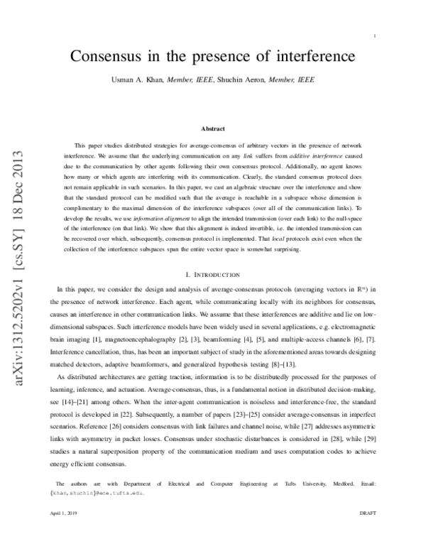Illustration of Theorem 1 In essence, Theorem 1 can be summarized in the following steps, illustrated with the help of Fig. 2: (i) Project the data, Rn , on a γ-dimensional subspace, S, via the projection matrix, IS . In Fig. 2 (a), the data (initial conditions) lies arbitrarily in R3 projected on a γ = 2-dimensional subspace, S, in Fig. 2 (b). Interference is given by a rank 1 matrix, Γ1 ; the interference subspace is shown by the black line; (ii) Align the projected subspace, S, on the null space, ΘΓ1 , of interference, Γ1 , via the preconditioning, T1 . In Fig. 2 (c), the projected subspace, S, is aligned to the null of space, ΘΓ1 , of the interference via preconditioning with T1 . Note that after the alignment, the data is orthogonal to the interference subspace (black line); (iii) Consensus is implemented now on the null space of the interference, see Fig. 2 (d). (iv) Recover the average in S via T1−1 . Finally, the average in the null space, ΘΓ1 , is translated back to the the signal subspace, S, via T1−1 . We also show the true average in R3 by the ‘⋆’, see Fig. 2 (e). From Theorem 1, when Γ1 is full-rank, i.e. γ = 0, the iterations converge to a zero-dimensional subspace and are not meaningful. However, if the interference is low-rank, consensus under uniform interference may still remain meaningful. In fact, we can establish the following immediate corollaries. April 1, 2019 DRAFT 9 (a) Fig. 2. (b) (c) (d) (e) Consensus under uniform interference: (a) Signal space, R3 , data shown as squares and the average as ‘⋆’; (b) Projected signal subspace, S, shown as circles and the average as ‘⋄’; (c) Alignment on the null space of the interference, T1 IS xi0 ; (d) Consensus in the null bik , average shown as large filled circle; and, (e) Translation back to the signal subspace, T1−1 x bi∞ . space of the interference, x Corollary 1 (Perfect Consensus). Let xi0 ∈ Rn be such that dim(⊕i xi0 ) ≤ dim(ΘΓ1 ). Then consensus under uniform interference, Eq. (14), recovers the true average of the initial conditions, xi0 . Corollary 2 (Principal/Selective Consensus). Let the initial conditions, xi0 , belong to the range space, ⊕A, of some matrix, A ∈ Rn×n . Then consensus under uniform interference, Eq. (14), recovers the average in a γ = dim(ΘΓ1 ) subspace that can be chosen along any γ singular values of A. The proofs of the above two corollaries immediately follow from Theorem 1. In fact, the protocol, Eq. (14), can be tailored towards the γ largest singular values (principal consensus), or towards any arbitrary γ singular values (selective consensus). The former is applicable to the cases when the data (initial conditions) lies primarily along a few singular values. While the latter is applicable to the cases when the initial conditions are known to have meaningful components in some singular values. We now show a few examples on this approach. Example 1. Consider the initial conditions, xi0 , ∀i, to lie in the range space, ⊕A, with the following:       −1 −1 1 1 √ √ 1 1 1 2 .  , IS =  2 2  , U S =  2 A= 1 1 −1 2 √1 √ 1 1 2 2 2 2 Clearly, dim(⊕A) = 1. Consider any rank 1 interference, Γ:     1 1 1 ,  , Θ Γ1 = β  Γ1 = α  −1 1 1 (18) α, β ∈ R. It can be easily verified that originally the data subspace, ⊕A, is aligned with the interference subspace, ⊕Γ1 , and standard consensus operation is not applicable as no agent knows from which agents and on what links this interference is being incurred (recall Assumption (a) in Section III). In other words, each agent i, implementing P P P Eq. (9), cannot ensure that j∈Ni wij + j∈Ni wij m∈V am ij = 1 for the above iterations to remain meaningful and convergent. Following Theorem 1, we choose T1 = V1 US⊤ , which can be verified to be a diagonal matrix with 1 and −1 on the diagonal, resulting into Γ1 T1 IS = 02×2 . The effect of preconditioning, T1 , is to move the entire 1-dimensional April 1, 2019 DRAFT 10 signal subspace in the null space of the interference. Subsequently, X X X bjk + 0n , bm bjk + bik+1 = wij x bm wij x x i Γ1 x k = j∈Ni when bi0 x = T1 IS xi0 = T1 xi0 , j∈Ni m∈V and true average is recovered via T1−1 (see Corollary 1). C. A Conservative Generalization In Section IV-A, we assume that the overall interference structure, recall Fig. 1, is such that the interference gains are uniform, i.e. Γm ij = Γ1 . We now provide a conservative generalization of Theorem 1 to the case when the interferences do not have a uniform structure. Theorem 2. Define Γ ∈ Rn×n to be the network interference matrix such that ⊕i,j,m Γm ij ⊆ ⊕ Γ, i, j, m, ∈ V. (19) Let ΘΓ be the null space of Γ with γ = dim(ΘΓ ). The protocol in Eq. (11) recovers the average in a γ-dimensional subspace, S, of Rn , with an appropriate alignment. The proof follows directly from Lemmas 1, 2, and Theorem 1. Following the earlier discussion, we choose a global preconditioning, T ∈ Rn×n , based on the null-space, ΘΓ , of the network interference, Γ. The solution described by Theorem 2 requires each interference to belong to some subspace of the network interference, ⊕Γ, and each agent to have the knowledge of this network interference. However, this global knowledge is not why the approach in Theorem 2 is conservative, as we explain below.
n m Consider ⊕i,j, Γm ij ⊆ R , to be such that dim ⊕Γij = 1, for each i, j, m ∈ V. In other words, each interference block in Fig. 1 is a one-dimensional line in Rn . Theorem 2 assumes a network interference matrix, Γ, such that its m range space, ⊕Γ, includes every local interference subspace, ⊕Γm ij . When each local interference subspace, ⊕Γij , is one-dimensional, we can easily have dim(⊕i,j,m Γm ij ) = n, subsequently requiring dim(⊕Γ) = n. This happens when the local interference subspaces are not aligned perfectly. Theorem 1 is a very special scenario when all of the local interference subspaces are exactly the same (perfectly aligned). Extending it to Theorem 2, however, shows that when the local interference are misaligned, ⊕Γ may have dimension n, and consensus is only ensured on a zero-dimensional subspace, i.e. with IS = 0n×n . This limitation of Theorem 2 invokes a significant question: When all of the local interferences are misaligned such that their collection spans the entire Rn , can consensus recover anything meaningful? Is it true that Theorem 2 is the only candidate solution? In the next sections, we show that there are indeed distributed and local protocols that can recover meaningful information. To proceed, we add another assumption, (c), to Assumptions (a) and (b) in Section III: (c) The interference matrices, Γm ij , are independent over j. Note that in our interference model, any agent m ∈ V can interfere with j → i communication; from Assumption (a), these are unknown to either agent j or i. Assumption (c) is equivalent to saying that this interference is only a function of the interferer, m ∈ V, or the receiver, i ∈ V, and is independent of communication link, j → i. April 1, 2019 DRAFT 11 We consider the design and analysis in the following cases: Uniform Outgoing Interference: Γm i = Γm , ∀i, m ∈ V. In this case, each agent, m ∈ V, interferes with every other agent via the same interference matrix, Γm , see Fig. 3 (top). This case is discussed in Section V; Uniform Incoming Interference: Γm i = Γi , ∀i, m ∈ V. In this case, each agent i incurs the same interference, Γi , j Fig. 3. m1 m2 m3 Tm1 Tm2 Tm2 m1 m2 Γ Γ Tj i m1 Interference Channel Interference Channel over all the interferers, m ∈ V, see Fig. 3 (bottom). This case is discussed in Section VI. m3 Γ Γi m3 Γl j l Tj m2 Ri i Rl l (Top) Uniform Outgoing (Bottom) Uniform Incoming. The blocks, Ti ’s and Ri ’s, will become clear from Sections V and VI. V. U NIFORM O UTGOING I NTERFERENCE This section presents results for the uniform outgoing interference, i.e. each agent, m ∈ V, interferes with every other agent in the same way. Recall that agent j wishes to transmit xj to agent i in the presence of interference. When this interference depends only on the interfere, agent i receives xjk + X m am ij Γm xk , (20) m∈V em eik ∈ from agent j at time k. We modify the transmission as Tm x k , for all m ∈ V for some auxiliary state variable, x Rn , to be explicitly defined shortly; agent i thus receives ejk + Tj x X m∈V em am ij Γm Tm x k , from agent j at time k. Consider the following protocol: eik+1 x = X Wij j∈Ni ejk Tj x + X m∈V em am ij Γm Tm x k (21) ! , (22) where Wij ∈ Rn×n is now a matrix that agent i associates with agent j; recall that earlier Wij = wij In . We get where Bim = P j∈Ni eik+1 = x X j∈Ni ejk + Wij Tj x X m∈V Wij am ij . We have the following result. em Bim Γm Tm x k , (23) Lemma 3. For some non-negative integer, γ ≤ n, let each outgoing interference matrix, Γi , have rank γ , n − γ. Let IS ∈ Rn×n be the projection matrix that projects Rn on S, where dim(S) = γ. Then, there exist Ti at April 1, 2019 DRAFT 12 each i ∈ V, and Wij ’s for all (i, j) ∈ E such that Eq. (23) becomes at each i ∈ V, when ei0 x X eik+1 = x ∈ S. j∈Ni ejk , wij x Proof: Without loss of generality, we assume that S = ⊕A, where ⊕A denotes the range space of some matrix, A ∈ Rn×n , such that dim(⊕A) = γ. Define IS = A† A, where IS is the orthogonal projection that projects ei0 , IS xi0 . Let Ti be the locally ei0 to be the projected initial conditions, i.e. x any arbitrary vector in Rn on S. Define x designed, invertible preconditioning, obtained at each i ∈ V from the null-space, ΘΓi , of its outgoing interference ei0 = 0n , ∀i ∈ V. Choose matrix, Γi , see Lemma 2. Clearly, following Lemma 2, we have Γi Ti x Wij = wij Tj−1 . (24) From Eq. (23), we have eik+1 = x X j∈Ni ejk + wij x X m∈V em Bim Γm Tm x k . ei0 ∈ S, ∀i ∈ V, then x eik ∈ S, ∀i ∈ V, k, proven below by induction. Consider k = 0, then We claim that when x ei1 = x X j∈Ni ej0 + wij x X m∈V em Bim Γm Tm x 0 = X j∈Ni ej0 , wij x eik ∈ S, ∀i ∈ V, and some k, leading which is a linear combination of vectors in S and thus lies in S. Assume that x eik = 0n . Then for k + 1: to Γi Ti x eik+1 = x X j∈Ni ejk + wij x which is a linear combination of vectors in S. X m∈V em Bim Γm Tm x k = X j∈Ni ejk , wij x The main result on uniform outgoing interference is as follows. Theorem 3. Let ΘΓi denote the null space of Γi , and let γ , mini∈V {dim(ΘΓi )}. In the presence of uniform outgoing interference, Eq. (22) recovers the average in a γ-dimensional subspace, S, of Rn , when we choose Ti according to Lemma 2, and Wij = wij Tj−1 , at each i, j ∈ Ni . The proof follows from Lemma 3. In other words, the consensus protocol in the presence of uniform outgoing interference, Eq. (22), converges to ei∞ = x N N 1 X j 1 X e0 = x IS xj0 , N j=1 N j=1 (25) for any xi0 ∈ Rn , ∀i ∈ V. We note that each agent, i ∈ V, is only required to know the null-space of its outgoing interference, Γi , to construct an appropriate preconditioning, Ti . In addition, each agent, i ∈ V, is required to obtain the local pre-conditioners, Tj ’s, only from its neighbors, j ∈ Ni ; and thus, this step is also completely local. April 1, 2019 DRAFT 13 (a) (b) (c) (d) Fig. 4. Consensus under uniform outgoing interference: (a) Signal space, S ⊆ R3 , where dim(S) = 2; (b) One-dimensional range spaces, ⊕Γi , of Γi ’s–the null spaces of each are γ = 2-dimensional, shown as planes; (c) Agent transmissions aligned in the corresponding null spaces over time, k; (d) Consensus in the signal subspace, S, after appropriate translations, at each i ∈ V, back to the signal subspace by Tj−1 , with j ∈ Ni . The protocol described in Theorem 3 can be cast in the purview of Fig. 3 (top). Notice that a transmission from any agent, i ∈ V, passes through agent i’s dedicated preconditioning matrix, Ti . The network (both noninterference and interference) sees only Ti xik at each k. Since the interference is a function of the transmitter (uniform outgoing), all of the agents ensure that a particular signal subspace, S, is not corrupted by the interference channel. The significance here is that even when the interferences are misaligned such that ⊕i∈V Γi = Rn , the protocol in Eq. (22) recovers the average in γ = mini∈V {ΘΓi } dimensional signal subspace. On the other hand, the null space of the entire collection, ⊕i∈V Γi , may very well be 0-dimensional. For example, if each Γi is rank 1 such that each of the corresponding one-dimensional subspace is misaligned, Eq. (22) recovers the average in an n − 1 dimensional signal subspace. On the other hand, Theorem 2 does not recover anything other than 0n . A. Illustration of Theorem 3 Let the initial conditions belong to a 2-dimensional subspace in R3 and consider N = 10 agents, with random initial conditions, shown as blue squares in Fig. 4 (a). Uniform outgoing interference is chosen as one of the three 1dimensional subspaces such that each interference appears at some agent in the network, see Fig. 4 (b). Clearly, each interference is misaligned and dim(⊕i Γi ) = n = 3. Hence, the protocol following Theorem 2 requires the signal subspace to be n − dim(⊕i Γi ) = 0 dimensional. However, when the agent transmissions are preconditioned using Ti ’s, each agent projects its transmission on the null space of its interference. Each receiver, i ∈ V, receives a misaligned data, Tj xj , from each of its neighbors, j ∈ Ni , see Fig. 4 (c). Since each Tj xj is a function of the corresponding neighbor, j, the data can be translated back to S via Tj−1 , which is incorporated in the consensus weights, Wij = wij Tj−1 . VI. U NIFORM I NCOMING I NTERFERENCE In this section, we consider the case of uniform incoming interference, i.e. each agent i ∈ V incurs the same interference, Γi , over all of the interferers, m ∈ V. This scenario is shown in Fig. 3 (bottom). We note that April 1, 2019 DRAFT 14 Theorem 2 is applicable here but results into a conservative approach as elaborated earlier. We note that this case is completely different from the uniform outgoing case (of the previous section), since preconditioning (alone) may not work as we explain below. When an agent, m ∈ V, employs preconditioning, it may not precondition to account for the interference, Γi , experienced at each receiver, i, with which m may interfere. In the purview of Fig. 3 (bottom), if agent m2 ∈ V preconditions using Tm2 to cancel the interference, Γi , experienced by agent i; the same preconditioning, Tm2 , is not helpful to agent l. For example, let agent m2 choose Tm2 = Vi US⊤ (a valid choice following Lemma 2), then as discussed earlier Γi Vi US⊤ IS = 0n×n and m2 ’s interference is not seen by agent i. However, this preconditioning appears as Γl Vi US⊤ IS at agent l, which is 0n×n only when Vl⊤ Vi = In . This is not true in general. We now explicitly address the uniform incoming interference scenario. In this case, Eq. (11) takes the following form: xik+1 = X xjk Wij X + Γi m am ij xk m∈V j∈Ni ! , (26) k ≥ 0, xi0 ∈ Rn and where, as in Section V, we use a matrix, Wij ∈ Rn×n to retain some design flexibility. The only possible way to cancel the unwanted interference now is via what can be referred to as post-conditioning. Each agent, i ∈ V, chooses a post-conditioner, Ri ∈ Rn×n . As before, we assume IS = US SS VS⊤ to be the bm projection matrix for some subspace, S ⊆ Rn , and modify the transmission as SS x k , for some auxiliary state bik ∈ Rn , to be explicitly defined shortly. The modified protocol is variable, x bik+1 x = X bjk SS x Wij Ri j∈Ni + Γi X m∈V bm am ij SS x k ! . (27) The goal is to design an Ri such that Ri Γi = 0n×n . Following the earlier approaches, we assume that rank(Γi ) = γ, ∀i ∈ V, and rank(IS ) = γ, such that γ + γ = n, with SVDs, Γi = Ui Si Vi⊤ and IS = US SS VS⊤ , where the singular value matrices are arranged as  Si1:γ Si =  0γ×γ   , 0γ×γ SS =  The next lemma characterizes the post-conditioner, Ri . Iγ  . (28) Lemma 4. Let Γi = Ui Si Vi⊤ and SS have the structure of Eq. (28). Given the null-space of Γ⊤ i , there exists a rank γ post-conditioner, Ri , such that Ri Γi = 0n×n . Proof: We assume that Ui is partitioned as the null-space of Γ⊤ i . Define h R i = SS ′ Ui | Ui h ′ i , where U i ∈ Rn×γ and U i ∈ Rn×γ . Clearly, U i is U i | U ′i i⊤ , (29) where U ′i is such that ⊕U ′i = ⊕U i , and U i is arbitrary. By definition, we have U ⊤ i U i = 0γ×γ ; hence, by April 1, 2019 DRAFT 15 ⊤ construction, U ′i U i = 0γ×γ . It can be verified that the post-conditioning results into   0 0  Vi⊤ , Ri Γi =  1:γ ′⊤ I γ U i U i Si 0 and the lemma follows. Note that Ri = SS Ui⊤ is a valid choice but it is not necessary. With the help of Lemma 4, Eq. (27) is now given by bik+1 x = X j∈Ni Wij SS h i⊤ ′ U i | U ′i bjk . SS x (30) Recall that U ′i is an n × γ matrix whose column-span is the same as the column-span of U i , and the column-span ′ b of U i is the null-space of Γ⊤ i . We now denote the lower γ × γ sub-matrix of U i by Ui . In order to simply the above iterations, we note that SS h ′ U i | U ′i i⊤ SS  0γ×γ  = b⊤ U i  , (31) b ⊤ is always invertible. Based on this and dim(U ′i ) = dim(U i ) = n − γ = γ. It is straightforward to show that U i discussion, the following lemma establishes the convergence of Eq. (27). Lemma 5. Let Γi = Ui Si Vi⊤ , ∀i ∈ V, and some projection matrix, IS = US SS VS⊤ , have ranks γ, and γ , n − γ, respectively (0 ≤ γ ≤ n), such that Si and SS are arranged as in Eq. (28). When Ri is chosen according to Lemma 4, and for each i ∈ V, Wij is chosen as  Wij = wij  0γ×γ  b⊤ U i  −1  , (32) bi0 . the protocol in Eq. (27) recovers the average of the last γ components of the initial conditions, x Proof: We note that under the given choice for Ri ’s, the interference term is 0n , and Eq. (27) reduces to Eq. (30). Now we use Eqs. (31) and (32) in Eq. (30) to obtain: bik+1 = x X j∈Ni bjk = Wij SS Ui⊤ SS x which in the limit as k → ∞ converges to bi∞ x = X j∈Ni  N 1 X  0γ×γ N j=1  wij  Iγ  0γ×γ x bi0 , Iγ  x bj , k ∀i ∈ V. (33) b ⊤ is invertible is always true because it is a principal minor of an invertible matrix, U ⊤ . That U i i Following is the main result of this section. Theorem 4. Let Γi ’s, Ri ’s, and Wij ’s, be chosen according to Lemma 5. The protocol in Eq. (27) under uniform incoming interference recovers the average in a γ-dimensional subspace, S, of Rn . April 1, 2019 DRAFT 16 Proof: Without loss of generality, assume that S has a projection matrix, IS , with SVD as defined above. bi0 = VS⊤ xi0 and define x eik = US x bik , ∀i ∈ V. Then, from Lemma 5 Let x   N N X X 0 1  γ×γ  VS⊤ xi0 = 1 ei∞ = US x US SS VS⊤ xi0 , N j=1 N Iγ j=1 ∀i ∈ V, and the theorem follows. Some remarks are in order to explain the mechanics of Theorem 4. Let IS = US SS VS⊤ with VS = h i and US = U S | U S , where V S is the null space of IS . h VS | VS i bm (i) When any agent i ∈ V receives SS x 0 as an interference, it is canceled via the post-conditioning by Ri , bm regardless of the transmission, SS x 0 : ⊤ bm bm R i Γi S S x SS x 0 = SS Si V i 0 = 0n , because of the structure in the SS and Si from Eq. (28). (ii) It is more interesting to observe the effect on the intended transmission, j → i, after the post-conditioning bj0 instead and multiplication with Wij . It is helpful to note that SS = SS† , and consider the transmission as SS† x bj0 : of SS x The operation, SS Ui⊤ , bj0 Wij Ri SS† x = Wij SS Ui⊤ | {z } Rx bj . SS† x | {z }0 Tx by the receiver, Rx, is vital to cancel the interference as shown in the previous step. However, this measure by the receiver also ‘distorts’ the intended transmission. What agent i receives is now bj0 and agent i multiplied by a low-rank matrix, SS† , in general. Consider for a moment that agent j were to send x bj0 , after the interference canceling operation. How can agent i choose an appropriate Wij to undo obtains SS Ui⊤ x this post-conditioning? Such a procedure is not possible unless in trivial scenarios, e.g., when the interference was a diagonal matrix and Ui = In . However, the transmitter may preemptively undo the distortion eventually incurred ej0 . by the receiver’s interference canceling operation. This is precisely what is achieved by sending SS† x ej0 , by the transmitter is vital so that the distortion (iii) As we discussed, a preemptive measure, sending SS† x bj0 may only bound to be added at the receiver is reversed. This reorientation, however, can be harmful, e.g., x contain meaningful (non-zero) information in the first γ components and the multiplication by SS destroys this bi0 = VS⊤ xi0 ; the first transmission information. To avoid this issue, we choose the initial condition at each agent as x at any agent i is thus: bi0 SS x =  SS VS⊤ xi0 =  0γ i V⊤ S x0  , which is to transform any arbitrary initial condition orthogonal to the null-space of the desired signal subspace, S. Since, the signal subspace, S, is γ-dimensional, retaining only the last γ components, after the transformation by VS⊤ , suffices. April 1, 2019 DRAFT , 17 (a) Fig. 5. (b) (c) (d) (e) Uniform Incoming Interference: (a) Signal subspace, S ⊆ R3 , with dim(S) = 2. The initial conditions are shown as blue squares and the true average is shown as a white diamond; (b) One-dimensional interference null-spaces at each agent, i ∈ V; (c) Auxiliary state ej0 = VS⊤ xi0 , shown as red circles; (d) Consensus iterates in the auxiliary states and the average in the auxiliary initial conditions; variables, x bik . eik = US x and, (e) Recovery via x (iv) We choose Wij according to Eq. (32) and obtain ∀i ∈ V, where xik bi1 = x X j∈Ni bj0 = SS VS⊤ Wij Ri SS x X j∈Ni wij xj0 = SS VS⊤ xi1 , bi2 , ignoring the interference terms are the interference-free consensus iterates. Now lets look at x as they are 0n , regardless of the transmission: bi2 = x X j∈Ni Wij Ri SS SS VS⊤ xj1 = SS VS⊤ xi2 , bik+1 = SS VS⊤ xik+1 , bi1 . In fact, the process continues and we get x by the same procedure that we followed to obtain x bi∞ = US SS VS⊤ xi∞ = IS xi∞ . ei∞ = US x bi∞ = SS VS⊤ xi∞ , and the average in S, is obtained by x or x A. Illustration of Theorem 4 We now provide a graphical illustration of Theorem 4. The network is comprised of N = 10 agents each with a randomly chosen initial condition on a 2-dimensional subspace, S, of R3 , shown in Fig. 5 (a). Incoming interference is chosen randomly as a one-dimensional subspace at each agent, shown as grey lines in Fig. 5 (b). It can be easily verified that the span of all of the interferences, ⊕i∈V Γi , is the entire R3 . The initial conditions are now transformed bik , does not destroy the signal subspace, S. This transformation is shown with VS⊤ so that the transmission, SS x bik , Fig. 5 (d), and finally, the in Fig. 5 (c). Consensus iterations are implemented in this transformed subspace, x eik , in the signal subspace, S, are obtained via a post-multiplication by US . iterations, x VII. D ISCUSSION We now recapitulate the development in this paper. Assumptions: The exposition is based on three assumptions, (a) and (b) in Section III, and (c) in Section IV-C. Assumption (a), in general, ensures that the setup remains practically relevant, and further makes the averaging problem non-trivial. Assumption (b) is primarily for the sake of simplicity; the strategies described in this paper are applicable to the time-varying case. What is required is that when any incoming (or outgoing) interference April 1, 2019 DRAFT 18 subspace changes with time, this change is known to the interferer (or the receiver) so that appropriate pre- (or post-) conditioning is implemented. Finally, Assumption (c) is noted to cast a concrete structure on the proposed interference modeling. In fact, one can easily frame the incoming or outgoing interference as a special case of the general framework. However, explicitly noting it establishes a clear distinction among the different structures. Conservative Paradigm: We consider a special case when each of the interference block in the network, see Fig. 1, is identical. This approach, rather restrictive, sheds light on the information alignment notion that keeps recurring throughout the development, i.e. hide the information in the null space of the interference. When the local interferences, Γm ij , are not identical, we provide a conservative solution that utilizes an interference ‘blanket’ (that covers each local interference subspace) to implement the information alignment. However, as we discussed, this interference blanket soon loses relevance as it may be n-dimensional to provide an appropriate cover. When this is true, the only reliable data hiding is via a zero-dimensional hole (origin) and no meaningful information is transmitted. This conservative approach is improved in the cases of uniform outgoing and incoming interference models. Uniform Outgoing Interference: The fundamental concept in the uniform outgoing setting is to hide the desired signal in the null-space of the interferences, Γm ’s. This alignment is possible at each transmitter as the eventual interference is only a function of the transmitter. Uniform Incoming Interference: The basic idea here is to hide the desired signal in the null-space of the transpose of incoming interferences, Γ⊤ i ’s. This alignment is possible at each receiver as the eventual interference is only a function of the receiver. It can be easily verified that the resulting procedure is non-trivial. Null-spaces: Incoming and outgoing interference comprise the two major results in this paper. It is noteworthy that both of these results only assume the knowledge of the corresponding interference null-spaces; the basis vectors of these null spaces can be arbitrary while the knowledge of the interference singular values is also not required. It is noteworthy that in a time-varying scenario where the basis vectors of the corresponding null-spaces change such that their span remains the same, no time adjustment is required. Uniform Link Interference: One may also consider the case when Γm ij = Γij , see Eq. (11), i.e., each interference gain is only a function of the communication link, j → i. Subsequently, when each receiving agent, i ∈ V, knows the null space of Γ⊤ ij , a protocol similar to the uniform incoming interference can be developed. Performance: To characterize the steady-state error, denoted by ei∞ at an agent i, define ei∞ = xi∞ − IS xi∞ , where xi∞ is the true average, Eq. (10). Clearly,
⊤ IS xi∞ ei∞ = (xi∞ )⊤ IS⊤ (In − IS ) xi∞ = 0, ∀i ∈ V, i.e. the error is orthogonal to the estimate, or the average obtained is the best estimate in S ⊆ Rn of the perfect average. VIII. C ONCLUSIONS In this paper, we consider three particular cases of a general interference structure over a network performing distributed (vector) average-consensus. First, we consider the case of uniform interference when the interference April 1, 2019 DRAFT 19 subspace is uniform across all agents. Second, we consider the case when this interference subspace depends only on the interferer (transmitter), referred to as uniform outgoing interference. Third, we consider the case when the interference subspace depends only on the receiver, referred to as uniform incoming interference. For all of these cases, we show that when the nodes are aware of the complementary subspaces (null spaces) of the corresponding interference, consensus is possible in a low-dimensional subspace whose dimension is complimentary to the largest interference subspace (across all of the agents). For all of these cases, we derive a completely local information alignment strategy, followed by local consensus iterations to ensure perfect subspace consensus. We further provide the conditions under which this subspace consensus recovers the exact average. The analytical results are illustrated graphically to describe the setup and the information alignment scheme. R EFERENCES [1] K Sekihara and S S Nagarajan, Adaptive spatial filters for electromagnetic brain imaging, Chapter 7: Effects of low-rank interference. 2008. [2] D Gutiérrez, Arye Nehorai, and A Dogandzic, MEG source estimation in the presence of low-rank interference using cross-spectral metrics, vol. 1, IEEE, 2004. [3] K Sekihara, S S Nagarajan, D Poeppel, and A Marantz, “Performance of an MEG adaptive-beamformer source reconstruction technique in the presence of additive low-rank interference,” Biomedical Engineering, IEEE Transactions on, vol. 51, no. 1, pp. 90–99, 2004. [4] M McCloud and L L Scharf, “Interference identification for detection with application to adaptive beamforming,” Conference Record of Thirty-Second Asilomar Conference on Signals, Systems and Computers, vol. 2, pp. 1438–1442 vol.2, 1998. [5] A Dogandzic, “Minimum variance beamforming in low-rank interference,” in Signals, Systems and Computers, 2002. Conference Record of the Thirty-Sixth Asilomar Conference on. 2002, pp. 1293–1297, IEEE. [6] R Lupas and S Verdu, “Linear multiuser detectors for synchronous code-division multiple-access channels,” Information Theory, IEEE Transactions on, vol. 35, no. 1, pp. 123–136, Jan. 1989. [7] M K Varanasi and A Russ, “Noncoherent decorrelative detection for nonorthogonal multipulse modulation over the multiuser Gaussian channel,” Communications, IEEE Transactions on, vol. 46, no. 12, pp. 1675–1684, Dec. 1998. [8] L L Scharf and Benjamin Friedlander, “Matched subspace detectors,” Signal Processing, IEEE Transactions on, vol. 42, no. 8, pp. 2146–2157, Aug. 1994. [9] M McCloud and L L Scharf, “Generalized likelihood detection on multiple access channels,” Conference Record of the Thirty-First Asilomar Conference on Signals, Systems and Computers (Cat. No.97CB36163), vol. 2, pp. 1033–1037 vol.2, 1997. [10] J Scott Goldstein and Irving S Reed, “Reduced-rank adaptive filtering,” Signal Processing, IEEE Transactions on, vol. 45, no. 2, pp. 492–496, Feb. 1997. [11] Xiaodong Wang and H V Poor, “Blind multiuser detection: a subspace approach,” Information Theory, IEEE Transactions on, vol. 44, no. 2, pp. 677–690, Mar. 1998. [12] A Dogandzic and Benhong Zhang, “Bayesian Complex Amplitude Estimation and Adaptive Matched Filter Detection in Low-Rank Interference,” Signal Processing, IEEE Transactions on, vol. 55, no. 3, pp. 1176–1182, 2007. [13] Fabian Monsees, Carsten Bockelmann, Mark Petermann, Armin Dekorsy, and Stefan Brueck, “On the Impact of Low-Rank Interference on the Post-Equalizer SINR in LTE,” Communications, IEEE Transactions on, vol. 61, no. 5, pp. 1856–1867, 2013. [14] A. Jadbabaie, J. Lin, and A. S. Morse, “Coordination of groups of mobile autonomous agents using nearest neighbor rules,” IEEE Transactions on Automatic Control, vol. 48, no. 6, pp. 988–1001, Jun. 2003. [15] L. Xiao, S. Boyd, and S. Kim, “Distributed average consensus with least-mean-square deviation,” Journal of Parallel and Distributed Computing, vol. 67, pp. 33–46, 2005. [16] A. K. Das and M. Mesbahi, “Distributed linear parameter estimation in sensor networks based on Laplacian dynamics consensus algorithm,” in 3rd IEEE Communications Society Conference, Reston, VA, Sep. 2006, vol. 2, pp. 440–449. April 1, 2019 DRAFT 20 [17] I. D. Schizas, A. Ribeiro, and G. B. Giannakis, “Consensus in ad hoc WSNs with noisy links - part I: Distributed estimation of deterministic signals,” IEEE Transactions on Signal Processing, vol. 56, no. 1, pp. 350–364, Jan. 2008. [18] U. A. Khan, S. Kar, and J. M. F. Moura, “Higher dimensional consensus: Learning in large-scale networks,” IEEE Transactions on Signal Processing, vol. 58, no. 5, pp. 2836–2849, May 2010. [19] R. Olfati-Saber, “Kalman-consensus filter : Optimality, stability, and performance,” in 48th IEEE Conference on Decision and Control, Shanghai, China, Dec. 2009, pp. 7036–7042. [20] C. G. Lopes and A. H. Sayed, “Diffusion least-mean squares over adaptive networks: Formulation and performance analysis,” IEEE Transactions on Signal Processing, vol. 56, no. 7, pp. 3122–3136, Jul. 2008. [21] S. Kar, J. Moura, and H. Poor, “Distributed linear parameter estimation: Asymptotically efficient adaptive strategies,” SIAM Journal on Control and Optimization, vol. 51, no. 3, pp. 2200–2229, 2013. [22] L. Xiao and S. Boyd, “Fast linear iterations for distributed averaging,” Systems and Controls Letters, vol. 53, no. 1, pp. 65–78, Apr. 2004. [23] M. G. Rabbat, R. D. Nowak, and J. A. Bucklew, “Generalized consensus computation in networked systems with erasure links,” in 6th International Workshop on Signal Processing Advancements in Wireless Communications, New York, NY, 2005, pp. 1088–1092. [24] A. Kashyap, T. Basar, and R. Srikant, “Quantized consensus,” Automatica, vol. 43, pp. 1192–1203, Jul. 2007. [25] T. C. Aysal, M. Coates, and M. Rabbat, “Distributed average consensus using probabilistic quantization,” in IEEE 14th Workshop on Statistical Signal Processing, Maddison, WI, Aug. 2007, pp. 640–644. [26] S. Kar and J. M. F. Moura, “Distributed consensus algorithms in sensor networks with imperfect communication: Link failures and channel noise,” IEEE Transactions on Signal Processing, vol. 57, no. 1, pp. 355–369, 2009. [27] Y. Chen, R. Tron, A. Terzis, and R. Vidal, “Corrective consensus with asymmetric wireless links,” in 50th IEEE Conference on Decision and Control, Orlando, FL, 2011, pp. 6660–6665. [28] T. C. Aysal and K. E. Barner, “Convergence of consensus models with stochastic disturbances,” IEEE Transactions on Information Theory, vol. 56, no. 8, pp. 4101–4113, 2010. [29] B. Nazer, A. G. Dimakis, and M. Gastpar, “Local interference can accelerate gossip algorithms,” IEEE Journal of Selected Topics in Signal Processing, vol. 5, no. 4, pp. 876–887, 2011. [30] S. A. Jafar, “Interference Alignment: A New Look at Signal Dimensions in a Communication Network,” Foundations and Trends in Communications and Information Theory, vol. 7, no. 1, pp. 1–136, 2011. [31] R. A. Horn and C. R. Johnson, Matrix Analysis, Cambridge University Press, New York, NY, 2013. April 1, 2019 DRAFT