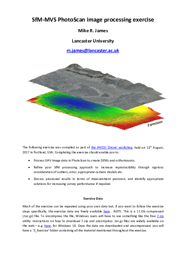
SfM-MVS PhotoScan image processing exercise Mike R. James Lancaster University The following exercise was compiled as part of the IAVCEI ‘Drone’ workshop, held on 13th August, 2017 in Portland, USA. Completing the exercise should enable you to: • • • Process UAV image data in PhotoScan to create DEMs and orthomosaics. Refine your SfM processing approach to increase reproducibility through rigorous consideration of outliers, error, appropriate camera models etc. Discuss processed results in terms of measurement precision, and identify appropriate solutions for increasing survey performance if required. Exercise Data Much of the exercise can be repeated using your own data but, if you want to follow the exercise steps specifically, the exercise data are freely available here . NOTE: This is a 11 Gb compressed (.tar.gz) file. To uncompress the file, Windows users will have to use something like the free 7-zip utility. Instructions on how to download 7-zip and uncompress .tar.gz files are widely available on the web – e.g. here, for Windows 10. Once the data are downloaded and uncompressed, you will have a ‘3_Exercise’ folder containing all the material mentioned throughout the exercise. IAVCEI 2017 – The Drone Workshop SfM-MVS PhotoScan image processing exercise Mike R. James Lancaster University This exercise was constructed using PhotoScan Pro v.1.3.2 and may not work with other versions. This exercise demonstrates how to process images into a 3-D model using PhotoScan software. It caters for users who are either unfamiliar with PhotoScan, or who have a reasonable working knowledge, with a focus on rigorous processing to understand and maximise model precision. These instructions were written using Agisoft PhotoScan Professional Edition v.1.3.2, and may not work fully with other versions. IAVCEI 2017 – The Drone Workshop PhotoScan exercise Mike James Contents 1 Introduction.................................................................................................................. 1 2 Initial 3-D model building ................................................................................................ 3 3 4 5 6 2.1 Add photos ............................................................................................................ 3 2.2 Assess image quality and remove poor images ............................................................ 4 2.3 Align photos ........................................................................................................... 5 Tie point quality control.................................................................................................. 7 3.1 Refine image selection............................................................................................. 7 3.2 Refine tie points by quality metrics ............................................................................ 7 3.3 Remove tie points manually...................................................................................... 8 Adding control data for georeferencing............................................................................. 8 4.1 Importing GCP ground survey data ............................................................................ 9 4.2 Making GCP image observations ..............................................................................10 4.3 Update georeference..............................................................................................10 4.1 Outlier image observations of GCPs ..........................................................................11 Bundle adjustment and camera model.............................................................................11 5.1 Weighting observations ..........................................................................................12 5.2 Camera model .......................................................................................................12 Dense matching, and DEM and orthomosaic products........................................................13 6.1 Dense matching .....................................................................................................13 6.2 Building a DEM ......................................................................................................14 6.3 Building an orthomosaic image ................................................................................15 7 Precision maps .............................................................................................................16 8 Finish ..........................................................................................................................18 9 References and resources ..............................................................................................19 IAVCEI 2017 – The Drone Workshop PhotoScan exercise Mike James 1 Introduction This exercise aims to give you experience in processing photographs into a 3-D model (and associated DEM and orthomosaic products) using PhotoScan software. It is intended to be accessible without prior experience in PhotoScan and to develop a rigorous approach when using SfM software, along with an understanding of characteristics such as measurement precision. Although based on a UAV-acquired dataset, the procedures are equally applicable to ground-based surveys. The exercise is split into sections, with each rated by the level of detail/complexity. If you just want a quick and easy 3-D visualisation, then completing o l the Basi aspects will suffice. I te ediate le el ate ial ill de elop a g eate i sight i to the underlying photogrammetric processing to enhance the repeatability of survey results, a d the ad a ed ate ial o e s considerations of measurement precision. Note that the exercise will not cover details specifically associated with very large projects e.g. >1000 images (such as working with multiple chunks). Following completion of the exercise, you should be able to:  Process images in PhotoScan into a georeferenced 3-D model and export associated point clouds, DEMs and orthomosaic products. [Basic]  Improve model quality by filtering images and tie points using quality metrics. [Intermediate]  Refine your processing by appropriately weighting observations during processing and checking for issues related to over-parameterisation of camera models. [Intermediate]  Describe what limits survey precision and, hence, how precision can be improved. [Advanced] Survey data: Data for the exercise a e p o ided o the o kshop s U“B, i the E e ise folde alo g ith a op of these instructions). The data are organised into sub-folders associated with the different sections of this document. The data are from a survey of aeolian gravel ripples that have formed since the eruption of Laki, Iceland. The ripples are composed of pumice (light-colored, low density) and basalt (dark-colored, high density), but the rate of sediment transport of these odd features is not known. An aerial survey of these ripples was acquired in 2015 using kite aerial photography, and again in 2016 using a common quadcopter, the DJI Phantom 3 Professional. The exercise is based on the 2016 UAVacquired dataset, kindly provided by Stephen Scheidt (Scheidt et al., 2017). http://www.dji.com/phantom-3-pro The UAV has a gimbal-stabilized FC300X camera containing the Sony EXMOR 1/2.3 sensor with a relatively wide field of view (FOV) of 94° (a 35 mm equivalent focal length of 20 mm). The JPEG images are compressed and 12 Megapixels in size (4000 x 3000), geotagged usi g the uad opte s a igatio al GPS and contain pointing information. The image survey was controlled by the Pix4Dapture app (https://pix4d.com/product/pix4dcapture/). 1 IAVCEI 2017 – The Drone Workshop PhotoScan exercise Mike James Prior to field deployment, base imagery from Google Earth was downloaded to the app (installed on an IPad Mini). In the field, a survey area was defined using the app by simply drawing a polygon on the map where a grid of images was desired. The app automatically estimated the maximum allo a le a ea of the su e usi g the uad opte s e pe ted flight ti e as a li iti g fa to . I this version of the app, a grid is defined assuming that two sets of orthogonal flights lines will be flown with the camera pointed slightly off-nadir. 50 m Two orthogonal sets of flight lines were flown (see left for an example area showing image positions by blue squares) with a forward-inclined camera to give a convergent imaging geometry between overlapping lines (e.g. James et al., 2014). With an approximate flight height of 30 m above ground, the camera delivered a nominal ground sampling distance (ground resolution) of ~1.3 cm. The area has virtually no vegetation, so the dataset should be a strong photogrammetric network revealing the exact topography of the surface sediments. Prior to the flight, orange survey cones were placed in the survey area as ground control points (GCPs), and their coordinates surveyed using a survey-grade R10 differential global positioning system (dGPS) from Trimble. Example images: Software and hardware requirements: The exercise assumes you have PhotoScan Professional Edition v.1.3.2 installed on suitable hardware (see here fo Agisoft s hardware recommendations, although these are quite generous!). Section 7 of the exercise additionally uses CloudCompare for visualising point clouds and, for an advanced optional extra, you may want to use sfm_georef to help visualise error. In the exercise, you will generate DEM and orthomosaic outputs, and you may want to use your favourite GIS/image analysis software to look at them in detail. 2 IAVCEI 2017 – The Drone Workshop PhotoScan exercise 2 Initial 3-D model building Mike James Level: Basic Completing this section should allow you to: Start PhotoScan and familiarise  Load photographs into PhotoScan. yourself with the different window  Assess images for quality and remove poor ones. panes in the application. If your  Generate an initial 3D model of sparse points. window does not have all the panes illustrated below, you can show them by using the main menu bar: View → Panes, and selecting any missing ones (e.g. Photos, ‘efe e e… . 2.1 Add photos To generate an initial 3-D point cloud model from photographs, we will use only a very few images from the full dataset, to accelerate the processing. To add photos to a project you can use the main menu bar: Workflow → Add Photos, or, alternatively, drag/drop the image files directly into the Workspace pane. Using either method, load the 18 images provided in the Section_2_Initial_model folder. The images should then appea i a Chu k i the Workspace pane a hu k is just a olle tio of images that will be processed together, along with the results). Expanding the project tree by clicking on it will give: 3 IAVCEI 2017 – The Drone Workshop PhotoScan exercise Mike James At this point, you should save your new project. From the main menu bar: File → Save as. Save the p oje t he e e ou a t, e su i g that the “a e as t pe: o is Photo“ a P oje t *.ps . 2.2 Assess image quality and remove poor images Photographs provide the underpinning data in a photogrammetric project so, to get high quality output, image quality should also be good – i.e. images should be crisp and not blurred. There are several ways to check:   For small surveys (e.g. <100 images), it is practical to check image quality visually. Doubleclick on the first image in the Photos pane to load and display the image. In the image pane that appea s, zoo i ouse heel to he k fo us a d lu i g. P essi g Page up / Page do ke s ill allow you to quickly navigate through all the images. For the images you have, there are some small variations in quality, but they are generally very good and certainly sufficient for processing. For large projects, PhotoScan has an image quality metric that can be a useful guide to highlight the poorest images. To calculate the metric, in the Photo pane, select an image, then right-click, and Esti ate I age Qualit … Apply to all cameras. The results can be viewed by changing the view style of the Photos pane, using the right-most button in the Panes toolbar to ha ge the ie to Details . Click on the Quality column header to order the images by quality. Any images with a quality score of <0.5 can probably be immediately removed, but you will see that yours all score much closer to 1.0 (maximum quality). To remove any poor images from the project, select them in the Photos pane and click the ‘e o e a e as button. Note that this only removes the image from the project, it does not delete the image file. 4 IAVCEI 2017 – The Drone Workshop PhotoScan exercise Mike James 2.3 Align photos You now have a set of reasonable-quality (or better) images. Before starting the image processing, it is worth noticing that PhotoScan already has some information on the positions of the camera in the survey. This information was extracted from EXIF metadata stored in the image file headers (and was originally written by the UAV system, which saved its GPS coordinates into each image). You can see this information in the Reference pane, where the camera position coordinates are given in the upper table. Camera positions can also be visualised in 3-D within the Model pane, via the main menu: View → Show/Hide Items → Show Cameras, or via the mai tool a “ho Ca e as utto . Finally, click on the Settings button in the Reference pane to bring up the Reference Settings dialog box. You will see that the Coordinate System is currently set to WGS 84, which appropriately reflects the GPS values for the camera positions. Close the dialog box. 5 IAVCEI 2017 – The Drone Workshop PhotoScan exercise Mike James To carry out “fM p o essi g to alig the a e as a d ge e ate a spa se -D point cloud, use the main menu: Workflow → Align photos. A dialog box will appear: For the General settings, we ll use High a u a hi h a e i o e ie tl slo fo e la ge surveys). Ensure that both Generic preselection and Reference preselection are ticked. Both of these speed up photo alignment (Reference preselection uses the preliminary camera position data to help select images to match and will not be available if camera positions are completely unknown). Advanced settings can be left at their default values. Start the processing, and when it is complete (hopefully in less than a few minutes), you should see something like this, showing the sparse cloud of 3-D tie points (grey) and aligned cameras (blue squares) in the Model pane: You may need to zoom in and out (mouse wheel) or scale the blue camera squares (shift-mouse wheel) to find the most useful visualisation). Save your project at this point, if you want to return to it. 6 IAVCEI 2017 – The Drone Workshop PhotoScan exercise 3 Tie point quality control The next processing step is to assess and refine the tie point quality, and will be explored using a fuller subset of the survey, which has been pre-aligned for you to save time. Thus, from folder Section_3_Tie_point_quality, open the project flight1_cropped.psx. Mike James Level: Intermediate Completing this section should allow you to:  Refine your survey by removing weakly matched images.  Refine your survey by removing weak or poor-quality tie points. This project provides 362 images for which cameras have been oriented and the sparse point cloud generated. However, although image quality data have been calculated, they have not yet been used to remove any poor images. 3.1 Refine image selection For image quality and other reasons, some images will not match as well as others and they can be removed from the project. Initially check for any images that might be removed by sorting the images by quality in the Photos pane and viewing a few of the poorest quality ones. Note that selecting images in the model Pane also highlights the appropriate rows in the Camera table of the Reference pane. In the Camera table, scroll to the right and sort the images by the Error (pix) column that gives the RMS tie point image residual for each image. By selecting poor-quality images in the Photos pane, you will see that they are often associated with large RMS tie point residual values (e.g. > 3 pix). Viewing the cameras in the Model pane also demonstrates that many are at unusual angles, suggesting that they were taken during manoeuvres between flight lines, where aircraft stability is likely to be reduced, and thus poor quality images more likely. Remove poor-quality images from the project – I removed 13 with the greatest RMS error, to leave 349. 3.2 Refine tie points by quality metrics The 3-D sparse point cloud will still contain tie points of varying quality, and overall results will be improved if low-quality tie points and obse atio s a e e o ed. Photo“ a p o ides a G adual “ele tio tool to help sele t a d e o e poi ts ased o a u e of diffe e t ualit et i s. I the Model pane, rotate the view so that you can see all the sparse points as clearly as possible (you may want to hide the cameras), then open the Gradual Selection tool from the main menu by Edit → Gradual sele tio … Cha ge the ite io to I age ou t . Mo e the slide to , which selects all the points that have only been observed in 3 or fewer images. Cli k OK , the hit the delete ke to remove these points. We have used 3 images here as a threshold due to the generally high overlap; in other projects you may need to use only 2. You can repeat this selection and filtering process using some of the other criteria listed below. App op iate th eshold alues ill a a d the e ill ot e a ight o e to use. Ho e e , g adual selection is a valuable tool to identify and remove points that are either outliers or at the weakest end of the quality distribution. Reprojection error: This metric represents image residuals, but is complicated by the fact that PhotoScan scales these values based on the image matching, so the do t di e tl efle t values in pixels for each point. Nevertheless, it is useful in order to identify and remove the worst points (largest values). 7 IAVCEI 2017 – The Drone Workshop PhotoScan exercise Mike James Reconstruction uncertainty: This is a complex metric that reflects how elongate the precision ellipse is on any point – large values indicate elongated ellipses (for UAV surveys, this usually indicates much weaker vertical precision than horizontal precision). Appropriate values to use as thresholds will vary between projects, and will depend on the number of images matched per point and the imaging geometry. P oje tio a u a : I ot e ti el lea o this o e…! F o the Photo“ a a ual: This criterion allows to filter out points which projections were relatively poorer localised due to thei igge size . It might be to do with the scale that points have been matched at. Following refinements, I had ~80,000 tie points remaining. At this point, it is worth checking that there are no images for which almost all observations have been removed. In the Reference pane, ie the P oje tio s olu i the Cameras; images with few observations (e.g. <500) would be good candidates for removal. Ideally, the distribution of such points, rather than their total number, should be the criterion for removal. PhotoScan does not currently offer a way to visualise tie point distributions but, if you are interested, it can be done using sfm_georef (James & Robson, 2012; James et al. 2017a). 3.3 Remove tie points manually In some circumstances, refinement through gradual selection can still leave some points which are clear outliers through being located far from the topographic surface, and these can be manually removed. To select points manually, in the Model pane, rotate the view so that you can see all the outlying sparse points as clearly as possible. Locate the selection tool in the main toolbar a d d op do the o to sele t the tool of hoi e I fi d the F ee-fo “ele tio the most useful). Click-drag in the Model pane to select the points you wish, and press the delete key to remove. Click the Navigation button to return the mouse to a navigation function rather than selection. 4 Adding control georeferencing data for Level: Basic-Intermediate Completing this section should allow you to:  Import GCP data and assign appropriate precision estimates.  Use image-matching assisted GCP identification to derive a preliminary georeference for your survey. If ou did t o plete the p e ious se tio , o want to start afresh, you can open the flight_1_cropped_refined.psx project in the Section_4_Adding_GCPs folder. You have seen that PhotoScan has some georeferencing information for camera positions from the on-board GPS data. These data have already been automatically used as control measurements - even without any GCPs in the project, the 3D model appears sensibly oriented and scaled. However, typically, these GPS data are rather poor precision (e.g. multiple metres) and suited only to relatively coarse metre-level georeferencing – which may be fine for some requirements, but not for many. PhotoScan assumes a default camera position precision of 10 m (as seen in the Reference Settings dialog box, and applied in X, Y and Z directions), which is probably appropriate. 8 IAVCEI 2017 – The Drone Workshop PhotoScan exercise Mike James Some UAV systems offer much greater precision from dual-frequency on-board receivers and can deliver centimetre-level survey precision. Detailed analyses of these types of di e tl geo efe e ed surveys are out of scope of this exercise. In using these camera position data, PhotoScan has detected (or assumed) that the camera coordinate values are in WGS 84 (latitude and longitude). To avoid conflict with GCP data provided in a different coordinate system, select all the cameras in the Reference pane (click on one row in the table, then press Control-A) and untick the check boxes. This deselects the camera position data from being used in any further georeferencing calculations. 4.1 Importing GCP ground survey data To precisely georeference this project, we will use GCPs which were deployed in the field as red cones. The coordinates of the NE corner of their bases were determined by survey-grade GPS. These GCP coordinates are provided in the file gcps_UTM_Zone_28N_WGS84.txt – open the file in a text editor to see the format (the columns are: label, X, Y, Z, sX, sY, sZ, where sX/Y/Z denotes the measurement precision in that coordinate). Note: If, in your own surveys, you do t have precisio information to import with GCP coordinates, the precision columns can be omitted and precision estimates set globally within PhotoScan later. To import the GCP data: 1) Click on the Import button in gcps_UTM_Zone_28N_WGS84.txt. the Reference toolbar and select 2) The GCP coordinates are given in UTM Zone 28N, WGS84 and this needs to be set as the coordinate system. Find the coordinate system goi g to Mo e… i the d opdo o the , under Projected Coordinate Systems, fi d Wo ld Geodeti “ ste a d sele t WG“ / UTM zone 28N (or use the filter box to search for 32628, the EPSG code!). Select the coordinate system and return to the Import CSV dialog box. 3) Ti k the A u a checkbox and set the accuracy column values to 5, 6 and 7 for Easting, Northing and Altitude respectively: 4) Click OK. PhotoScan will sa it a t fi d a at h o e isti g photo o a ke ith the sa e a e as the la els , so li k e a ke fo all . Note that the orientation of the model will 9 IAVCEI 2017 – The Drone Workshop PhotoScan exercise Mike James change, hi h is due to the ha ge i the p oje t s oo di ate s ste . You will see the imported GCP coordinates appear in the Markers table of the Reference pane. 4.2 Making GCP image observations With the ground survey GCP data imported, the GCPs now need to be located within the imagery. Firstly, to make sure that your manual GCP identifications will be aided by automated image matching, use the main menu: Tools → Preferences and, in the dialog box that comes up, go to the Advanced ta . E su e that Refine marker positions based on image content is he ked. Now, identify your first GCP in an image: i i age …DJI_ 056, look for the red cone of gcp-002 (just under half way across the image and about three quarters the way up the image). Zoom in to see the cone clearly, right click on the top right corner of the cone base, the sele t Pla e a ke …. g p-002. A white dot will appear at the point, attached to a green flag, denoting a pinned GCP observation. In the Reference panel, look on the right hand side of the Markers table, and you should see that a number of o se atio s ha e o ee auto ati all ade of that GCP the P oje tio s olu . If this has remained at 1, find the same GCP in another image (e.g. …DJI_ 057) to make another manual measurement. This time, you will be guided to its location by a striped line, along which PhotoScan is expecting the marker to be located. Find the GCP, and place the marker as before. With multiple observations, PhotoScan has sufficient information to estimate where a marker should be in other images. In the Reference pane, right click on the table entry for gcp-002, and select Filter Photos by Markers . The Photos pa e ill o o l list i ages i hi h this GCP is expected to be visible. With the Photos pane showing the image thumbnails, images in which an observation has been manually set (pinned) will be annotated with a green flag. Images in which the GCP has been identified by automated image matching are annotated with a blue flag, and grey furled flags indicate images in which the GCP is expected, but has not been manually identified or successfully located by image matching. Grey-flagged positions are not used in georeferencing calculations. Double-click on an image annotated by a grey furled flag in the Photos pane, then drag the marker into the appropriate position in the image (if you are confident you know where it should go!). This will pin the observation, as indicated by the green flag annotation in the Photos pane. Note: You do t have to convert all (or any) of the grey flags but aim for a minimum of ~5 observations per marker (easily exceeded in this project). Poor-quality observations are not usually worth it. Practice this process on two more GCPs before proceeding to Section 4.3: gcp-004: find it in …DJI_0101, (the cone is located above the centre of the image and, again, place the marker on top right hand corner of the cone base) gcp-007: find it in …DJI_0121, (as above, but with the cone located about a third the way across the image, and three quarters the way up. 4.3 Update georeference With three (or more) GCPs identified in multiple images, the survey can be georeferenced using these GCP observations. In the Reference panel, click on the Update button to recalculate the georeferencing transform. Update determines the best-fit transform of translation, rotation and scale, which links the 3-D GCP coordinates estimated from the photogrammetry to the 10 IAVCEI 2017 – The Drone Workshop PhotoScan exercise Mike James control coordinates (provided by the GPS survey). Thus, update does ot ha ge the shape of the 3-D model, just its size, position and orientation. You ill o see alues appea i the e o olu of the Ma ke s ta le, hi h ep ese t the isfit between the photogrammetric and the control data. If any are substantially larger than expected (e.g. metres in this case), then it is likely that a GCP has been incorrectly identified. The values you see should be somewhere in the 0.03 – 0.04 m range. The survey now has a preliminary georeference based on the GCPs identified in the images, and PhotoScan can estimate the positions of the remaining GCPs in images. For any remaining GCPs with no observations (except gcp-001), use the Filter photos by marker fu tio to e a le ou to lo ate the GCPs in the images. Note – ignore gcp-001 as it does not relate to a cone location! You might notice that PhotoScan estimated that gcp-005 was rather far from its location in the image and, having pinned the marker, it shows a much greater error than the others. This suggests that it is not consistent with all the other GCPs. Click the Update button again to re-calculate the transform. Error now increases overall (~0.17 m), and particularly on GCPs next to gcp-005 (4 and 6). Uncheck gcp-005 in the Markers table to remove it from georeferenceing calculations and re-run the update. RMS error on the control points should decrease to ~0.06 m, but error on gcp-005 (now used only as a check point) will be high – 0.66 m. This straightforward exploration of the error distribution on GCPs helps identify potential problems in the data – here, gcp-005 has been identified as being substantially less consistent with the photogrammetric model than all the other GCPs. 4.1 Outlier image observations of GCPs There are fewer options for analysing the image residuals on GCPs than for tie points, but the Markers table has an Error (pix) column that gives the RMS image residual value for each marker. Right-clicking on any entry in the Markers table will provide a context menu from which you can “ho i fo… . This information gives you the image residuals for all observations of that marker, and enables individual weak observations to be identified. Such observations can either be removed or adjusted by opening the appropriate image in the Image pane. 5 Bundle adjustment camera model and If you have not completed all the previous section, you can use the project flight1_cropped_refined_GCPs.psx, in the Section_5_Bundle_adjustment folder to start this section. Level: Intermediate-Advanced Completing this section should allow you to:  Fully optimise your project using bundle adjustment with ground control.   Appropriately weight the observations used in the adjustment. Recognise the potential problems with over-parameterisation of camera models. “o fa , usi g the Update utto has enabled your project to be georeferenced by using the GCP control data to scale and orient the model. However, the GCPs have not been used to help refine the shape of the model. By including 11 IAVCEI 2017 – The Drone Workshop PhotoScan exercise control data within the overall optimisation (the be optimised simultaneously. Mike James u dle adjust e t , shape and georeferencing can In PhotoScan, bundle adjustment is carried out via the Opti ize Ca e as utto o the Reference pane toolbar. Ensuring that all your GCPs are checked (active), click the Optimize Cameras button and then, leaving the selection of camera parameters at its default values, click OK. Following the adjustment, the RMS error on the control points should drop to ~0.13 m. 5.1 Weighting observations This optimization has been carried out using PhotoScan s default weighting of tie point and marker image observations (1.0 and 0.1 pix respectively). For this survey, these are not very good estimates of the actual image residuals – the RMS image residual on markers is given in the last column of the Marker table (and should be ~1.4 pix) and the RMS image residual for tie points can be found from the Workspace pane (right-click on the chunk in the project tree a d sele t Show info ; it should be ~1.3 pix). Thus, markers (GCPs) have been substantially over-weighted by using PhotoScan s default values. 1. To change the weightings, in the Reference pane, click on the Settings button, and edit the alues i the Image coordinates accuracy o app op iatel (e.g. 1.4 pix for Marker accuracy and 1.3 pix for Tie point accuracy ). 2. Re-run the bundle adjustment, and check that RMS image error values have not changed substantially. Small changes can be used to update the settings values and the adjustment run again, if required. 3. As you did previously, see how removing gcp-005 from the bundle adjustment (by unchecking its box) affects the results. Note down the total error values for control and check points. Do you think gcp-005 should be included in the adjustment? The importance of appropriate observation weighting will vary with the relative numbers/precisions /distributions of markers and tie points and, ultimately, with the accuracy requirements of the survey. If decimetric accuracy or better is required, then appropriate weighting may well be important. See James et al. (2017a) for more details and the impacts of inappropriate weighting. 5.2 Camera model We have not yet examined the camera model. In the main menu, go to Tools → Camera Cali ratio … to bring up the camera Calibration Window (right): Cli ki g o the Adjusted ta sho s the distortion parameter values that have been determined during the optimisation. These include k1-3 (radial distortion) and p1, p2 (tangential distortion). In many cameras, tangential distortion is very small and can often be neglected. 12 IAVCEI 2017 – The Drone Workshop PhotoScan exercise Mike James We will now see what the effect of removing tangential distortion from the camera model will be: 1. O the Adjusted ta , edit the p a d p alues to . a d li k OK . 2. Run the bundle adjustment again, ensuring that Fit p they will not be included in the optimisation. a d Fit p are unchecked so that 3. When the adjustment is complete, check the RMS on the control points and check points, which should now be something like 0.07 and 0.14 m respectively. So, the simpler camera model has resulted in a very slight increase in the overall error on the control points, but a substantial reduction (from ~0.66 m) on the independent check point. Thus, if the simplified camera model is used, the fit to the GCPs appears more generic. Nevertheless, the error on gcpdoes e ai ele ated, so it a ell still e a outlie . To esol e this, e d eall need additional GCPs deployed so that more could be used as independent check points. More advanced analysis of camera models can be carried out using visualisations accessed through the Camera Calibration window (see the previous image). In the Camera Calibration window, rightclick on the blue-highlighted camera group (top left) and select Distortio Plot…. This provides plots of the distortion model and the residuals as well as listing parameter values, precisions and correlations. A detailed discussion is out of scope here (see conventional photogrammetry literature) but, ideally, residuals should be small and randomly oriented. For more information on assessing over-parameterisation in SfM projects see James et al. (2017a, b). He e, I d suggest usi g the simplified camera model and leaving gcp-005 as a check point. 6 Dense matching, and DEM and orthomosaic products Level: Basic Completing this section should allow you to:  Generate a dense point cloud, and DEM and orthomosaic products. You have now completed the photogrammetric and georeferencing processing, which determines the shape of the survey along with the camera positions and models. Now these are fixed, then the dense matching can be undertaken (you can try this with any of your previous georeferenced projects). Dense matching does not change the survey shape or georeferencing and, if shape is subsequently adjusted (e.g. a further camera optimization is carried out) then the dense matching output will be discarded automatically. 6.1 Dense matching Dense matching uses the established survey geometry and camera models to generate many more 3-D points and can take many hours for a large project. Thus, here, we will select only a small region of the project to work from. To resize the area to be processed, click on the Resize Region button in the Reference toolbar, and move the corners of the bounding region (identified by the blue spheres in the Model pane) so that only a small area of the survey is encompassed by the region box. Click the Navigation button to return to Navigation mode. Now, from the main menu: Workflow → Build dense cloud. In the dialog box that appears, set the quality to Medium (higher quality gives more points, but is slower), and click OK. To ie the esult, li k the De se Cloud utto o the ai tool a : 13 IAVCEI 2017 – The Drone Workshop PhotoScan exercise Mike James 6.2 Building a DEM The dense point cloud provides the detailed topographic data needed for building a DEM. For maximum flexibility in DEM-building, you can export the dense point cloud (from the main menu, use File → Export Poi ts…) and process it in the software of your choice (e.g. a GIS package, Surfer et . . Alte ati el , ou a use Photo“ a s i uilt DEM tool. This works in two stages, firstly to construct an underlying DEM, then to resample and export this as required. To build the underlying DEM, from the main menu, go to Workflow → Build DEM. Note – it is t possi le to ha ge ost of the parameters here and your boundaries and total size (pix) values will vary depending on size of the region you selected. You get more options when you want to export the DEM Click OK. PhotoScan allows you to visualise your DEM (and ake so e si ple easu e e ts, hi h e o t cover here). To view the DEM, in the Workspace pane, double-click on the DEM item in the chunk to bring up the Ortho view tab. If you had generated a DEM of the full region, it would look like this (and you can visualise a full DEM in the next section): To export the DEM, from the main menu: File → E port DEM… and select the export file type that you want. At this point, you can change the DEM extent and resolution to suit your requirements. 14 IAVCEI 2017 – The Drone Workshop PhotoScan exercise Mike James 6.3 Building an orthomosaic image Once you have built a DEM, then you can also construct an orthomosaic image. Again, this works in two stages, building the orthomosaic and exporting it. From the main menu: Workflow → Build Ortho osai …, and the dialog box shown on the left will come up. Parameters here can be changed as required. However, orthomosaic processing can be slow, so a pre-processed project has been prepared for you in the Section_6_Dense_matching_DEMs_Ortho folder. Thus, to view a full DEM or orthomosaic image, open flight1_processed.psx, in which the dense matching, DEM and orthomosaic processing has already been carried out for the full survey (i.e. a larger region than you have been working on so far). Just as for DEMs, the orthomosaic can be viewed in the Ortho tab, by double-clicking on the orthomosaic item in the Workspace pane: To export an orthomosaic image from the main menu, use File → Export orthomosaic and select the export file type you want. 15 IAVCEI 2017 – The Drone Workshop PhotoScan exercise 7 Precision maps Mike James Level: Advanced Completing this section should allow you to: A key aspect of all measurement is  Consider the precision-limiting factors of a survey. the uncertainty involved. Some idea  Visualise point precision estimates using of survey uncertainty can be given CloudCompare. by the misfit error on control and check points. However, these are often spatially limited and, in the case of control points, error is not independent from the optimisation. In rigorous photogrammetric processing, precision estimates are provided for all optimised parameters, including the sparse point coordinates. Unfortunately, current SfM-based software does not generally offer this, but point coordinate precision can be estimated using PhotoScan and a Monte Carlo approach (James et al., 2017b). This Monte Carlo precision processing has been carried out for you on the full Flight1 survey. For your interest, the Python script used, precision_estimates.py and a processing output log _precision_log.txt are provided in the Section_7_Precision_estimates data folder. The _precision_log.txt file provides a number of statistics that characterise the overall precision of the survey. Full details are given in James et al. (2017b), but a few interesting ones to note are the relative precision ratios given at the end of the file. Here, mean point precision is given in terms of observation distance, overall survey extent and pixels. The values here support the overall quality of the survey – mean horizontal precision is ~1 pixel and vertical precision is ~2 pixels. Also in the Section_7_Precision_estimates folder are the two output files from the Monte Carlo processing which can be used to visualise how the survey precision varies spatially: _point_precision_and_covars.txt - full point coordinate precision estimates and covariance information. _point_precision_and_covars_shape_only.txt - point coordinate precision estimates and covariance information that exclude the uncertainty in overall survey georeferencing. If you have CloudCompare (or a similar point cloud visualisation application), you can import the data in these text file outputs as point clouds (import the X, Y, Z fields as point coordinates, the sX, sY, sZ fields as scalars and ignore the other fields – e o t o side o a ia e he e . B usi g the sZ scalar field to colour the point cloud, you can assess the variation in vertical precision across the su e , effe ti el ge e ati g a p e isio ap . “u h aps gi e i sight i to the su e pe fo a e, and indicate what aspects are limiting the precision achievable (James et al. 2017b). For the full precision estimates (_point_precision_and_covars.txt), you should be able to see something like this (GCP positions are overlain in black for reference): 16 IAVCEI 2017 – The Drone Workshop PhotoScan exercise Mike James 50 Precision, Z (mm) _point_precision_and_covars.txt 0 Note:   Precision is shown to generally vary smoothly so, overall, precision is being limited by the georeferencing. This is because, for the full survey, a large area lies outside the region covered by the GCPs. As you move away from the weighted centroid of the control measurements, precision will deteriorate because the effects of uncertainty in georeferencing scale and angular orientation become amplified. There are some localised areas which show poorer precision, and these can be assessed in more detail with the overall survey georeferencing uncertainty removed: 50 Precision, Z (mm) __point_precision_and_covars_shape_only.txt 0 Note:   The precision associated with survey shape only is generally worst at the survey edges where the number of overlapping images will be smallest. In the survey centre, image overlap does not appear to substantially limit precision (e.g. there is only some evidence of image overlap outlines). Other, more discrete areas of weak precision reflect ground features, so changes in image texture due to surface variations is having some identifiable effects on precision. 17 IAVCEI 2017 – The Drone Workshop PhotoScan exercise Mike James 8 Finish Having completed this exercise, you should now be able to:  Load images into PhotoScan, build a georeferenced 3-D model and export associated point clouds, DEMs and orthomosaic products.      Improve your survey quality by identifying and removing weak images and tie points. Identify GCPs that may have unacceptable error. Appropriately weight observations within the bundle adjustment (optimisation) in order to maximise the repeatability of a survey s esults. Consider the influence of differing camera models and carry out basic tests for overparameterisation. Interpret precision maps in terms of the precision-limiting factors affecting a survey and, hence, make suitable recommendations for improving survey precision. Fi all , he epo ti g ou o k… This exercise has focussed on the processing techniques that come after data acquisition but acquiring appropriate data starts by designing the image acquisition strategy to meet the survey requirements. Dimensionless estimates of precision can help guide survey design, for example, by using 1:1000 for mean precision : observation distance (James et al. 2012) as an initial guide. Further recommendations can be found in Eltner et al. , O Co o et al. a d Mos u ke et al. (2017). Dimensionless parameters also represent a valuable way to report survey quality, for example, giving precision ratios or precision expressed in pixels. PhotoScan provides some useful parameters in a processing report that can be generated from the main menu File → Ge erate Report… For more detailed analysis, see the precision processing logs generated along with precision maps (discussed in Section 7; James et al., 2017b). Such metrics should be used to clearly communicate the quality of your surveys. Happy flying! Any feedback on this exercise is welcome: 18 IAVCEI 2017 – The Drone Workshop PhotoScan exercise Mike James 9 References and resources Valuable additional information can be obtained from the PhotoScan website and manuals: PhotoScan: http://www.agisoft.com/ PhotoScan manuals : http://www.agisoft.com/downloads/user-manuals/ There are a wide range of additional resources on the web to get you started with PhotoScan (including tutorials on the PhotoScan website above), although many have somewhat different suggestions! Those from UNAVCO are recommended: Structure from Motion guide - Practical survey considerations. Structure from Motion AgiSoft processing guide This exercise was based on Data: Scheidt, S. P., Bonnefoy, L. E., Hamilton, C. W., Sutton, S., Whelley, P. and deWet, A. P. (2017) Remote sensing analysis of Askja pumice megaripples in the Vikursundar, Iceland as an analog for martian transverse aeolien ridges, Fifth Intl Planetary Dunes Workshop 2017, LPI Contrib. No. 1961, abstract 3020. Sfm-georef for visualising error: James, M. R. and Robson, S. (2012) Straightforward reconstruction of 3D surfaces and topography with a camera: Accuracy and geoscience application, J. Geophysical Res., 117, F03017, doi: 10.1029/2011JF002289 Survey design for itigati g syste atic error do i g : James, M. R. and Robson, S. (2014) Mitigating systematic error in topographic models derived from UAV and ground-based image networks, Earth Surf. Proc. Landforms, 39, 1413–1420, doi: 10.1002/esp.3609 Rigorous processing, detailed GCP analysis and assessment of camera over-parameterisation: Ja es, M. ‘., ‘o so , “., d Olei e-Oltmanns, S. and Niethammer, U. (2017a) Optimising UAV topographic surveys processed with structure-from-motion: Ground control quality, quantity and bundle adjustment, Geomorphology, 280, 51–66, doi: 10.1016/j.geomorph.2016.11.021 Precisio aps a d u dersta di g survey precisio : James, M. R., Robson, S., Smith, M. W. (2017b) 3-D uncertainty-based topographic change detection with structure-from-motion photogrammetry: precision maps for ground control and directly georeferenced surveys, Earth Surf. Proc. Landforms, accepted, February, doi: 10.1002/esp.4125 19 IAVCEI 2017 – The Drone Workshop PhotoScan exercise Mike James Photogrammetry books Ultimately, to improve SfM-MVS results though a deeper understanding of photogrammetric processing, recourse to standard text books is fully recommended; some excellent example are: Krauss, K. (1993) Photogrammetry, Vol. 1, Fundamentals and Standard Processes, Dümmlers. Luhmann ,T., Robson, S., Kyle S. and Harley I. (2006) Close Range Photogrammetry: Principles, Methods and Applications, Whittles, Caitness. McGlone, J. C. (2013) Manual of Photogrammetry, American Society for Photogrammetry and Remote Sensing, Bethesda. Wolf, P.R., Dewitt., B.A. and Wilkinson, B. E. (2014) Elements of Photogrammetry with Applications in GIS, McGraw-Hill Education. Good data collection Good results are underpinned by good data collection. These papers discuss some of the imaging issues and also make recommendations for rigorous (and open) reporting of acquisition parameters: Eltner, A., Kaiser, A., Castillo, C., Rock, G., Neugirg, F. and Abellán, A. (2016) Image-based surface reconstruction in geomorphometry – merits, limits and developments, Earth Surf. Dynam., 4, 359–389, doi:10.5194/esurf-4-359-2016 Mosbrucker, A. R., Major, J. J., Spicer, K. R. and Pitlick, J. (2017) Camera system considerations for geomorphic applications of SfM photogrammetry, Earth Surf. Proc. Landforms, 42, 969-986, doi: 10.1002/esp.4066 Cameras and settings for aerial surveys in the O Co o , J. “ ith, M. a d Ja es, M. ‘. geosciences: Optimising image data, Prog. Phys. Geog., doi: 10.1177/0309133317703092 Work using UAVs and SfM-MVS in the geosciences There is a huge number of relevant papers – here are very a few of the early/interesting ones as a sample from a range of active groups: Eltner, A., Baumgart, P., Maas, H.-G., and Faust, D. (2015) Multi-temporal UAV data for automatic measurement of rill and interrill erosion on loess soil, Earth Surf. Proc. Land., 40, 741–755. Harwin, S., Lucieer, A., Osborn, J., (2015) The impact of the calibration method on the accuracy of point clouds derived using unmanned aerial vehicle multi-view stereopsis. Remote Sens., 7, 11933–11953. Hugenholtz, C. H., Whitehead, K., Brown, O. W., Barchyn, T. E., Moorman, B. J., LeClair, A., Riddell, K. and Hamilton, T. (2013) Geomorphological mapping with a small unmanned aircraft system (sUAS): Feature detection and accuracy assessment of a photogrammetricallyderived digital terrain model, Geomorphology, 194, 16–24 Immerzeel, W. W., Kraaijenbrink, P. D. A., Shea, J. M., Shrestha, A. B., Pellicciotti, F., Bierkens, M. F. P. and de Jong, S. M. (2014) High-resolution monitoring of Himalayan glacier dynamics using unmanned aerial vehicles, Remote Sens. Environ., 150, 93–103. Nakano T., Kamiya I., Tobita M., Iwahashi, J. and Nakajima, H. (2014) Landform monitoring in active volcano by UAV and SfM-MVS technique. ISPRS-Int. Arch. Photog. Rem. Sens. Spat. Info. Sci., XL-8, 71–75. Niethammer, U., James, M. R, Rothmund, S. and Joswig M. (2012) UAV-based remote sensing of the Super-Sauze landslide: Evaluation and results, Engineering Geology, 128, 2-11, Turner, D., Lucieer, A. and Wallace, L. (2014) Direct georeferencing of ultrahigh-resolution UAV imagery. IEEE Trans. Geosci. Remote Sens., 52, 2738–2745. 20 IAVCEI 2017 – The Drone Workshop PhotoScan exercise Mike James SfM-MVS work by the author on active volcanic systems The first SfM-MVS work on active lava flows and domes: James, M. R., Applegarth, L. J. Pinkerton, H. (2012) Lava channel roofing, overflows, breaches and switching: insights from the 2008-9 eruption of Mt. Etna, Bull. Volc., 74, 107-117, doi: 10.1007/s00445-011-0513-9. James, M. R. and Varley, N. (2012) Identification of structural controls in an active lava dome with high resolution DEMs: Volcán de Colima, Mexico, Geophys. Res. Letts., 39, L22303, doi:10.1029/2012GL054245. Rhyolite emplacement dynamics: Tuffen, H., James, M. R., Castro, J. M. & Schipper, C. I. (2013) Exceptional mobility of a rhyolitic obsidian flow: observations from Cordón Caulle, Chile, 2011-2013, Nat. Comms., 4, 2709, doi: 10.1038/ncomms3709 Farquharson, J., James, M. R. and Tuffen, H. (2015) Examining rhyolite lava flow dynamics through photo-based 3-D reconstructions of the 2011-2012 lava flowfield at Cordón Caulle, Chile, J. Volcanol. Geotherm. Res., 304, 336-348 doi: 10.1016/j.jvolgeores.2015.09.004 Stereo time-lapse DEMs of lava emplacement: James, M. R. and Robson, H. (2014) Sequential digital elevation models of active lava flows from ground-based stereo time-lapse imagery, ISPRS J. Photogram. Remote Sens., 97, 160-170, doi: 10.1016/j.isprsjprs.2014.08.011 3-D models from thermal imagery of lava dome growth: Thiele S. T., Varley, N. and James, M. R. (2017) Thermal photogrammetric imaging: a new technique for monitoring dome eruptions, J. Volcanol. Geotherm. Res., doi: 10.1016/j.jvolgeores.2017.03.022 21