Proof Complexity of Non-Classical Logics⋆
Olaf Beyersdorff1 and Oliver Kutz2
1
2
Institut für Theoretische Informatik, Leibniz-Universität Hannover, Germany
beyersdorff@thi.uni-hannover.de
Research Center on Spatial Cognition (SFB/TR 8), Universität Bremen, Germany
okutz@informatik.uni-bremen.de
Abstract. Proof complexity is an interdisciplinary area of research utilising techniques from logic, complexity, and combinatorics towards the
main aim of understanding the complexity of theorem proving procedures. Traditionally, propositional proofs have been the main object of
investigation in proof complexity. Due their richer expressivity and numerous applications within computer science, also non-classical logics
have been intensively studied from a proof complexity perspective in the
last decade, and a number of impressive results have been obtained.
In these notes we give an introduction to this recent field of proof complexity of non-classical logics. We cover results from proof complexity of
modal, intuitionistic, and non-monotonic logics. Some of the results are
surveyed, but in addition we provide full details of a recent exponential
lower bound for modal logics due to Hrubeš [60] and explain the complexity of several sequent calculi for default logic [16, 13]. To make the
text self-contained, we also include necessary background information on
classical proof systems and non-classical logics.
⋆
Part of these notes are based on the survey [12] and the research paper [13]. This
paper was produced while the first author was visiting Sapienza University of Rome
under support of grant N. 20517 by the John Templeton Foundation. The work of
the second author was supported by the DFG-funded Research Centre on Spatial
Cognition (SFB/TR 8), project I1-[OntoSpace].
�Table of Contents
1 Introduction . . . . . . . . . . . . . . . . . . . . . . . . . . . . . . . . . . . . . . . . . . . . . . . . . . .
1.1 Propositional Proof Complexity . . . . . . . . . . . . . . . . . . . . . . . . . . . . .
1.2 Proof Complexity of Non-Classical Logics . . . . . . . . . . . . . . . . . . . .
1.3 Organisation of the Paper and Guidelines for Reading . . . . . . . . . .
2 Preliminaries I: Classical Proof Complexity . . . . . . . . . . . . . . . . . . . . . . . .
2.1 Frege Systems and Their Extensions . . . . . . . . . . . . . . . . . . . . . . . . .
2.2 The Propositional Sequent Calculus . . . . . . . . . . . . . . . . . . . . . . . . .
3 Preliminaries II: Non-classical Logics . . . . . . . . . . . . . . . . . . . . . . . . . . . . .
3.1 Modal Logic and Kripke Semantics . . . . . . . . . . . . . . . . . . . . . . . . . .
3.2 Intuitionistic Logic and Semantics . . . . . . . . . . . . . . . . . . . . . . . . . . .
3.3 Default Logic . . . . . . . . . . . . . . . . . . . . . . . . . . . . . . . . . . . . . . . . . . . . .
4 Interpolation and the Feasible Interpolation Technique . . . . . . . . . . . . . .
4.1 Interpolation in Classical and Non-Classical Logic . . . . . . . . . . . . .
4.2 Feasible Interpolation . . . . . . . . . . . . . . . . . . . . . . . . . . . . . . . . . . . . . .
5 Lower Bounds for Modal and Intuitionistic Logics . . . . . . . . . . . . . . . . . .
5.1 Sketch of the Lower Bound . . . . . . . . . . . . . . . . . . . . . . . . . . . . . . . . .
5.2 Lower Bounds for Intuitionistic Logic . . . . . . . . . . . . . . . . . . . . . . . .
5.3 The Modal Clique-Colour Tautologies . . . . . . . . . . . . . . . . . . . . . . . .
5.4 Modal Assignments . . . . . . . . . . . . . . . . . . . . . . . . . . . . . . . . . . . . . . . .
5.5 A Characteristic Set of Horn Clauses . . . . . . . . . . . . . . . . . . . . . . . .
5.6 A Version of Monotone Interpolation for K . . . . . . . . . . . . . . . . . . .
5.7 The Lower Bound . . . . . . . . . . . . . . . . . . . . . . . . . . . . . . . . . . . . . . . . .
6 Simulations between Non-Classical Proof Systems . . . . . . . . . . . . . . . . . .
7 Proof Complexity of Default Logic . . . . . . . . . . . . . . . . . . . . . . . . . . . . . . .
7.1 Complexity of the Antisequent and Residual Calculi . . . . . . . . . . .
7.2 Proof Complexity of Credulous Default Reasoning . . . . . . . . . . . . .
7.3 On the Automatisability of BOcred . . . . . . . . . . . . . . . . . . . . . . . . . .
7.4 A General Construction of Proof Systems for Credulous
Default Reasoning . . . . . . . . . . . . . . . . . . . . . . . . . . . . . . . . . . . . . . . . .
7.5 Lower Bounds for Sceptical Default Reasoning . . . . . . . . . . . . . . . .
8 Discussion and Open Problems . . . . . . . . . . . . . . . . . . . . . . . . . . . . . . . . . .
3
3
4
5
6
10
12
13
14
18
22
26
26
27
29
31
31
32
32
33
36
37
37
41
41
44
46
46
48
50
�3
1
Introduction
These notes originate in an ESSLLI course held in August 2010 at the University
of Copenhagen. The aim of this course was—and is of these notes—to present an
up-to-date introduction to proof complexity with emphasis on non-classical logics
and their applications. The ESSLLI course started with a first lecture introducing
central concepts from classical proof complexity and then concentrated in the
remaining four lectures on proof complexity of non-classical logics. The material
here is organised slightly differently, but again we will start with some remarks
on the motivations for proof complexity, first for classical propositional proofs
and then for proof complexity of non-classical logics.
1.1
Propositional Proof Complexity
One of the starting points of propositional proof complexity is the seminal paper
of Cook and Reckhow [34] where they formalised propositional proof systems as
polynomial-time computable functions which have as their range the set of all
propositional tautologies. In that paper, Cook and Reckhow also observed a fundamental connection between lengths of proofs and the separation of complexity
classes: they showed that there exists a propositional proof system which has
polynomial-size proofs for all tautologies (a polynomially bounded proof system)
if and only if the class NP is closed under complementation. From this observation the so called Cook-Reckhow programme was derived which serves as one of
the major motivations for propositional proof complexity: to separate NP from
coNP (and hence P from NP) it suffices to show super-polynomial lower bounds
to the size of proofs in all propositional proof systems.
Although the first super-polynomial lower bound to the lengths of proofs had
already been shown by Tseitin in the late 60’s for a sub-system of Resolution
[105], the first major achievement in this programme was made by Haken in
1985 when he showed an exponential lower bound to the proof size in Resolution for a sequence of propositional formulae describing the pigeonhole principle
[55]. In the last two decades these lower bounds were extended to a number
of further propositional systems such as the Nullstellensatz system [7], Cutting
Planes [18, 91], Polynomial Calculus [32, 95], or bounded-depth Frege systems
[1, 8, 9, 78]. For all these proof systems we know exponential lower bounds to
the lengths of proofs for concrete sequences of tautologies arising mostly from
natural propositional encodings of combinatorial statements.
For proving these lower bounds, a number of generic approaches and general
techniques have been developed. Most notably, there is the method of feasible
interpolation developed by Krajı́ček [73], the size-width trade-off introduced by
Ben-Sasson and Wigderson [10], and the use of pseudorandom generators in
proof complexity [2, 74, 75].
Despite this enormous success many questions still remain open. In particular
Frege systems currently form a strong barrier [17], and all current lower bound
methods seem to be insufficient for these strong systems. A detailed survey of
recent advances in propositional proof complexity is contained in [101].
�4
Let us mention that the separation of complexity classes is not the only
motivation for studying lengths of proofs. In particular concerning strong systems such as Frege and its extensions there is a fruitful connection to bounded
arithmetic which adds insights to both subjects (cf. [72]). Further, understanding weak systems such as Resolution is vital to applications as for example the
design of efficient SAT solvers (see e. g. [90] for a more elaborate argument).
Last but not least, propositional proof complexity has over the years grown into
a mature field and many researchers believe that understanding propositional
proofs and proving lower bounds—arguably the hardest task in complexity—is
a very important and beautiful field of logic which is justified in its own right.
1.2
Proof Complexity of Non-Classical Logics
Besides the vivid research on propositional proof complexity briefly mentioned
above, the last decade has also witnessed intense investigations into the complexity of proofs in non-classical logics. Before describing some of the results, let
us comment a bit on the motivation for this research. Rudolf Carnap formulated
his Principle of Logical Tolerance in 1934 [30], endorsing a pragmatic choice of
logical formalism that is most beneficial for a given scientific endeavour. Since
then, computing science has gone a long way, and logical methods are being
employed in almost all areas of modern computer science. As a consequence,
logical pluralism understood pragmatically is today common sense. Here is one
such voice [85] articulating this position:
[. . . ] it is a fact of life that no single perspective, no single formalisation or level
of abstraction suffices to represent a system and reason about its behaviour.
[. . . ] no logical formalism (specification language, prototyping language, etc.)
will be best for all purposes. What exists is a space of possibilities (the universe
of logics) in which careful choice of the formalisms that best suit some given
purposes can be exercised.
Non-classical logics can therefore be considered even more important for computer science than classical logic as they adapt to needed expressive capabilities
and hence are often more suitable for concrete applications.
Whilst such heterogeneity might be rather obvious when considering quite
different application areas across computer science, say formal verification vs.
database theory, it materialises also within a single domain. Consider the case of
formal ontology engineering. Here, ontologies are being designed in lightweight
description logics (DLs) suitable e.g. for very large biomedical ontologies, expressive DLs (for smaller more expressive domain ontologies), and first-order logic
(e.g. foundational ontologies). However, also intuitionistic logic is being used (e.g.
concerning legal ontologies) as well as paraconsistent logic for handling inconsistent information, and non-monotonic and default logic for handling rules and
�5
exceptions. Of course, each such logic comes with specialised reasoning support
and quite distinct proof systems.3
Given this situation, it is therefore rather important to enhance our understanding of theorem proving procedures in these logics, in particular, given the
impact that lower bounds to the lengths of proofs have on the performance of
proof search algorithms. From the list of logics just mentioned, besides classical logic we will consider here in detail the modal logic K (and some of its
extensions), intuitionistic logic INT, as well as Reiter’s default logic.
Another motivation comes from complexity theory. As non-classical logics
are often more expressive than propositional logic, they are usually associated
with large complexity classes like PSPACE. The satisfiability problem in the
modal logic K was shown to be PSPACE-complete by Ladner [82], and this was
subsequently also established for many other modal and intuitionistic logics.4
Thus, similarly as in the Cook-Reckhow programme mentioned above, proving
lower bounds to the lengths of proofs in non-classical logics can be understood as
an attempt to separate complexity classes, but this time we are approaching the
NP vs. PSPACE question. Intuitively therefore, lower bounds to the lengths of
proofs in non-classical logic should be easier to obtain, as they “only” target at
separating NP and PSPACE. In some sense the results of Hrubeš [60] and Jeřábek
[65] on non-classical Frege systems (see Section 5) confirm this intuition: they
obtain exponential lower bounds for modal and intuitionistic Frege systems (in
fact, even extended Frege) whereas to reach such results in propositional proof
complexity we have to overcome a strong current barrier [17].
Last not least, research in non-classical proof complexity will also advance our
understanding of propositional proofs as we see a number of phenomena which
do not appear in classical logic (as e. g. with respect to the question of Frege vs.
EF and SF , see Section 6). These results are very interesting to contrast with
our knowledge on classical Frege as they shed new light on this topic from a
different perspective.
1.3
Organisation of the Paper and Guidelines for Reading
The remaining part of these notes is organised as follows. We start with two
preliminary sections on classical propositional proof systems and non-classical
logics, respectively. These two sections contain all definitions and notions that
are used in the text. In particular, Section 2 on proof complexity contains definitions and results on propositional proof systems such as Resolution, Frege,
and LK . In Section 3, we provide background material for modal, intuitionistic,
and default logic. In Section 4, we explain interpolation, both in classical logic
3
4
The broad logical landscape found in contemporary ontology engineering is described
in detail in [81].
In fact, PSPACE seems to be the “typical” complexity of monomodal logics and
similar systems which we will consider here. The complexity often gets higher for
logics in richer languages, e. g., PDL or the modal µ-calculus, but we are not aware
of any proof complexity research on these, though.
�6
and in modal and intuitionistic logics. Building on interpolation, the feasible
interpolation technique is one of the main techniques for lower bounds in proof
complexity. This technique is described in Section 4.2.
Proof complexity of non-classical logics properly starts in Section 5. In Section 5, we discuss strong lower bounds for modal and intuitionistic logics. In
particular, we give full details on the exponential lower bound for K due to
Hrubeš [60]. In Section 6, we survey simulations between modal and intuitionistic Frege systems. Section 7 is devoted to the proof complexity of propositional
default logic where again we give full details. Finally, we conclude in Section 8
with some open problems.
The reader familiar with proof complexity and/or non-classical logic may
skip Sections 2 and 3 (and possibly even Section 4 on interpolation) and directly proceed to the main material in Sections 5 to 7. Sections 5–7 are almost
independent and can be read in any order.
2
Preliminaries I: Classical Proof Complexity
We fix a language of propositional connectives. In most places the actual choice
of these connectives is not important as long as they form a basis for the set of
all boolean functions. In the following, we will allow the connectives ∧, ∨, →, ¬
and constants 0,1. The set TAUT is defined as the set of all propositional tautologies over these connectives. Sometimes we will also consider proof systems
for tautologies over a restricted propositional language. To better distinguish
propositional tautologies from tautologies in other logics we will also alternatively denote TAUT by PL.
Propositional proof systems were defined in a very general way by Cook
and Reckhow in [34] as polynomial-time computable functions P which have as
its range the set of all tautologies. In fact, their definition applies to arbitrary
languages.
Definition 1 (Cook, Reckhow [34]). A proof system for an arbitrary language L is a polynomial-time computable function P with rng(P ) = L. Proof
systems for L = TAUT are called propositional proof systems.
�
A string π with P (π) = ϕ is called a P -proof of the element ϕ. The intuition
behind this definition is that given a proof it should be easy to determine which
formula is actually proven and to verify the correctness of the proof. Nevertheless
it might be difficult to generate proofs for a given formula and proofs might be
very long compared to the size of the formula proven.
Probably the simplest propositional proof system is the truth-table system
that proves formulae by checking all propositional assignments. In the sense of
Definition 1 proofs in the truth-table system consist of the proven formula ϕ to|Var(ϕ)|
. As most formulae require exactly exponential proof
gether with a string 12
size in this system it is neither very interesting from the application oriented nor
from the proof complexity perspective.
�7
But also all the usually studied proof systems are captured by the above
definition. Let us illustrate this by an example. One of the most widely used
proof systems is the Resolution calculus and its variants introduced by Davis and
Putnam [37] and Robinson [99]. Resolution is a refutation system that operates
with clauses which are finite sets of negated or unnegated variables called literals.
A clause is associated with the disjunction of the literals it contains and a set of
clauses is associated with the conjunction of its clauses. Therefore finite sets of
clauses correspond to propositional formulae in conjunctive normal form.
A clause is satisfied by a propositional assignment if at least one literal of the
clause is satisfied by the assignment. Therefore by definition the empty clause
is unsatisfiable. A Resolution proof shows the unsatisfiability of a set of clauses
by starting with these clauses and deriving new clauses by the Resolution rule
C ∪ {p}
D ∪ {¬p}
C ∪D
until the empty clause is derived.
At first glance the Resolution system does not seem to fit into the CookReckhow framework of propositional proof systems because it is a refutation
system and can furthermore only refute formulae in CNF. But we can associate
with Resolution the following function Res:
Res(π) =
ϕ
⊤
if π = (ϕ, C1 , . . . , Ck ) where ϕ is a formula in DNF
and C1 , . . . Ck is a Resolution refutation of the set
of clauses for ¬ϕ
otherwise.
The second line of the definition is incorporated because by definition every string
π has to be interpreted as a proof of some formula. Clearly, Res is computable
in polynomial time. Hence in accordance with the above general definition, Res
is a proof system for all propositional tautologies in DNF. A common way to
extend the Resolution system from a proof system for formulae in DNF to a proof
system for all propositional tautologies is to transfer the formula to an equivalent
formula in DNF, either by direct translation or by using new auxiliary variables
(cf. [26] for the details).
Proof systems can be compared according to their strength by the notion
of simulation. In proof complexity, simulations play a similar role as reductions
in computational complexity. Given two proof systems P and S for the same
language L, we say that S simulates P (denoted by P ≤ S) if there exists a
polynomial p such that for all x and P -proofs π of x there is a S-proof π ′ of
x with |π ′ | ≤ p (|π|) [76]. If such a proof π ′ can even be computed from π in
polynomial time we say that S p-simulates P and denote this by P ≤p S [34].
If P ≤ S, then we will often simply say that S is stronger than P . As usual we
say that P and S are equivalent (denoted by P ≡ S) if P ≤ S and S ≤ P . The
relation ≡p is defined similarly. It is clear that ≡ and ≡p are equivalence relations
on the set of all proof systems. Their equivalence classes are called degrees.
�8
A proof system is called (p-)optimal if it (p-)simulates all proof systems.
Whether or not optimal proof systems exist is an open problem posed by Krajı́ček
and Pudlák [76].
The central objective in proof complexity is to understand how long proofs
have to be for a given formula. There are two measures which are of primary
interest. The first is the minimal size of an f -proof for some given element x ∈ L.
To make this precise, let
sf (x) = min{ |w| | f (w) = x }
and
sf (n) = max{ sf (x) | |x| ≤ n, x ∈ L } .
We say that the proof system f is t-bounded if sf (n) ≤ t(n) for all n ∈
N. If t is a polynomial, then f is called polynomially bounded. Another
interesting parameter of a proof is the length defined as the number of proof
steps. This measure only makes sense for proof systems where proofs consist of
lines containing formulae or sequents. This is the case for most systems studied
in this paper. For such a system f , we let
tf (ϕ) = min{ k | f (π) = ϕ and π uses k steps }
and tf (n) = max{ tf (ϕ) | |ϕ| ≤ n, ϕ ∈ L }. Obviously, it holds that tf (n) ≤
sf (n), but the two measures are even polynomially related for a number of
natural systems as extended Frege (cf. [72]).
Given the general notion of a proof system from Definition 1, a proof system
for a language L is simply a nondeterministic procedure that accepts L. Hence
polynomially bounded proof systems correspond to NP-algorithms for L. This
connection to complexity theory is made precise by the following theorem of
Cook and Reckhow from their seminal paper [34].
Theorem 2 (Cook, Reckhow [34]). Let L be an arbitrary nonempty language. Then there exists a polynomially bounded proof system for L if and only
if L ∈ NP.
Proof. For the first direction let P be a polynomially bounded proof system for
L with bounding polynomial p. Consider the following algorithm:
1
2
3
Input: a string x
guess π ∈ Σ ≤p(|x|)
IF P (π) = x THEN accept ELSE reject
Obviously the above algorithm is a nondeterministic polynomial-time algorithm
for L, hence L ∈ NP.
For the other direction assume that L ∈ NP. Hence there exists a nondeterministic polynomial time Turing machine M that accepts L. Let the polynomial
p bound the running time of M . Consider the function
�
x
if π codes an accepting computation of M (x)
P (π) =
x0
otherwise
where x0 ∈ L is some fixed element. Then P is a proof system for L which is
polynomially bounded by p.
�
�9
Optimal Proof System?
ZFC
Extended
Frege
Frege
-----------------------------------------------------------------------
not polynomially
bounded
Boundeddepth Frege
Cutting
Planes
PCR
Resolution
Polynomial
Calculus
Tree-like
Resolution
Nullstellen
Satz
Truth Table
Fig. 1. The simulation order of propositional proof systems
By the coNP-completeness of TAUT, this means that there exists a polynomially bounded propositional proof system if and only if NP = coNP. From this
result the Cook-Reckhow programme is derived which we already mentioned in
the introduction. To separate NP from coNP (and hence also P from NP) it is
sufficient to establish for stronger and stronger propositional proof systems that
they are not polynomially bounded.
Figure 1 depicts some of the most common propositional proof systems together with their simulation relations. A line between proof systems indicates
that the lower proof system is simulated by the higher system in Fig. 1. Moreover all the proof systems below the dashed line have also been separated, i.e.
the simulations do not hold in the opposite direction. The dashed line shows the
current frontier in the search for super-polynomial lower bounds to the proof
length, i.e. for all systems below the line sequences of formulae are known that
do not admit polynomial size proofs in the respective proof systems, whereas for
the systems above the line there is currently no information about non-trivial
lower bounds to the proof size available. A detailed description of the proof sys-
�10
tems depicted in Fig. 1 together with information on lower bounds can be found
in the surveys [92], [101], and [106].
2.1
Frege Systems and Their Extensions
In this section we will describe Frege systems and their extensions. These are
strong proof systems that will play a central role for the rest of these notes.
Frege systems derive formulae using axioms and rules. In texts on classical
logic these systems are usually referred to as Hilbert-style systems but in propositional proof complexity it has become customary to call them Frege systems
[34].
A Frege rule is a (k + 1)-tuple (ϕ0 , ϕ1 . . . , ϕk ) of propositional formulae
such that
{ϕ1 , ϕ2 , . . . , ϕk } |= ϕ0 .
The standard notation for rules is
ϕ1 ϕ 2
...
ϕk
ϕ0
.
A Frege rule with k = 0 is called a Frege axiom.
A formula ψ0 can be derived from formulae ψ1 , . . . , ψk by using the Frege
rule (ϕ0 , ϕ1 . . . , ϕk ) if there exists a substitution σ such that
σ(ϕi ) = ψi
for i = 0, . . . , k .
Let F be a finite set of Frege rules. An F-proof of a formula ϕ from a set of
propositional formulae Φ is a sequence ϕ1 , . . . , ϕl = ϕ of propositional formulae
such that for all i = 1, . . . , l one of the following holds:
1. ϕi ∈ Φ or
2. there exist numbers 1 ≤ i1 ≤ · · · ≤ ik < i such that ϕi can be derived from
ϕi1 , . . . , ϕik by a Frege rule from F.
We denote this by F : Φ ⊢ ϕ.
F is called complete if for all formulae ϕ
|= ϕ
⇐⇒
F :∅⊢ϕ .
F is called implicationally complete if for all ϕ ∈ Form and Φ ⊆ Form
Φ |= ϕ
⇐⇒
F :Φ⊢ϕ .
F is a Frege system if F is implicationally complete.
Without proof we note that the set of axioms and rules in Table 1, taken
from [26], constitute an example of a Frege system for classical propositional
logic PL. In the formulas in Table 1, we associate brackets from right to left,
i.e. p1 → p2 → p1 abbreviates p1 → (p2 → p1 ).
This definition leaves much freedom to design individual Frege systems but
if we are only interested in the lengths of proofs there is only one Frege system
F as already noted by Cook and Reckhow [34] (cf. also Section 6).
�11
Axioms
Rules
p 1 → p2 → p 1
(p1 → p2 ) → (p1 → (p2 → p3 )) → (p1 → p3 )
p 1 → p1 ∨ p 2
p 2 → p1 ∨ p 2
(p1 → p3 ) → (p2 → p3 ) → (p1 ∨ p2 → p3 )
(p1 → p2 ) → (p1 → ¬p2 ) → ¬p1
¬¬p1 → p1
p1 ∧ p 2 → p 1
p1 ∧ p 2 → p 2
p1 → p 2 → p 1 ∧ p2
p1
p1 → p2
p2
Table 1. A Frege system for propositional logic PL.
Theorem 3 (Cook, Reckhow [34]). Let F1 and F2 be Frege systems. Then
F1 ≡p F2 .
�
Now we describe the extensions of Frege systems as introduced in [34]. Let
F be a Frege system. An extended Frege proof of ϕ from a set Φ of formulae
is a sequence (ϕ1 , . . . , ϕl = ϕ) of propositional formulae such that for each
i = 1, . . . , l one of the following holds:
1. ϕi ∈ Φ or
2. ϕi has been derived by an F-rule or
3. ϕi = q ↔ ψ where ψ is an arbitrary propositional formula and q is a new
propositional variable that does not occur in ϕ, Φ, ψ, and ϕj for 1 ≤ j < i.
The introduction of the extension rule 3 allows the abbreviation of possibly
complex formulae by variables. Hence using this rule for formulae which appear
very often in an F-proof can substantially reduce the proof size.
Analogously as in Theorem 3 it follows that all extended Frege systems are
polynomially equivalent. It is clear that EF simulates Frege systems but whether
EF is indeed a strictly stronger system is an open problem.
Another way to enhance the power of Frege systems is to allow substitutions
not only for axioms but also for all formulae that have been derived in Frege
proofs. This is accomplished by introducing the substitution rule
ϕ
σ(ϕ)
which allows to derive σ(ϕ) for an arbitrary substitution σ from the earlier
proven formula ϕ. Augmenting Frege systems by this substitution rule we arrive
at the substitution Frege system SF .
�12
SF is polynomially equivalent to EF . While EF ≤p SF is relatively easy to
see [34] the transformation of SF -proofs to EF -proofs on the propositional level
is quite involved [76]. We will discuss this in more detail in Section 6.
2.2
The Propositional Sequent Calculus
Historically one of the first and best analysed proof systems is Gentzen’s sequent
calculus [48]. The sequent calculus is widely used both for propositional and firstorder logic. Here we will describe the propositional sequent calculus LK. The
basic objects of the sequent calculus are sequents
ϕ1 , . . . , ϕm −→ ψ1 , . . . , ψk .
Formally these are ordered pairs of two sequences of propositional formulae separated by the symbol −→. The sequence ϕ1 , . . . , ϕm is called the antecedent
and ψ1 , . . . , ψk is called the succedent. These cedents are usually denoted by
letters like Γ and ∆. An assignment α satisfies a sequent
Γ −→ ∆
if
α |=
_
ϕ∈Γ
¬ϕ ∨
_
ψ .
ψ∈∆
The sequence ∅ −→ ∆ having empty antecedent is abbreviated as −→ ∆. Likewise Γ −→ abbreviates Γ −→ ∅. Sequences of the form
A −→ A,
0 −→,
−→ 1
are called initial sequents. The sequent calculus LK uses the following set of
rules:
1. weakening rules
Γ −→ ∆
A, Γ −→ ∆
and
Γ −→ ∆
Γ −→ ∆, A
Γ1 , A, B, Γ2 −→ ∆
Γ1 , B, A, Γ2 −→ ∆
and
Γ −→ ∆1 , A, B, ∆2
Γ −→ ∆1 , B, A, ∆2
and
Γ −→ ∆1 , A, A, ∆2
Γ −→ ∆1 , A, ∆2
and
A, Γ −→ ∆
Γ −→ ∆, ¬A
2. exchange rules
3. contraction rules
Γ1 , A, A, Γ2 −→ ∆
Γ1 , A, Γ2 −→ ∆
4. ¬ : introduction rules
Γ −→ ∆, A
¬A, Γ −→ ∆
�13
5. ∧ : introduction rules
A, Γ −→ ∆
A ∧ B, Γ −→ ∆
and
A, Γ −→ ∆
B ∧ A, Γ −→ ∆
and
Γ −→ ∆, A
Γ −→ ∆, B
Γ −→ ∆, A ∧ B
6. ∨ : introduction rules
A, Γ −→ ∆
B, Γ −→ ∆
A ∨ B, Γ −→ ∆
and
Γ −→ ∆, A
Γ −→ ∆, A ∨ B
and
Γ −→ ∆, A
Γ −→ ∆, B ∨ A
7. cut-rule
Γ −→ ∆, A
A, Γ −→ ∆
Γ −→ ∆
Similarly as in Frege systems an LK-proof of a propositional formula ϕ is a
derivation of the sequent
−→ ϕ
from initial sequents by the above rules. Without proof we note that the above
set of rules specifies a proof system that is complete for the set of all tautologies
(see [72]).
As Frege systems can be easily transformed into the sequent formulation a
straightforward analysis shows that Frege systems and the Gentzen calculus LK
polynomially simulate each other.
Proposition 4 (Cook, Reckhow [34]). Frege systems and the propositional
sequent calculus LK are polynomially equivalent.
�
3
Preliminaries II: Non-classical Logics
In this section, we cover the basics of the non-classical logics whose proofcomplexity we analyse subsequently. This comprises basic syntax and semantics,
as well as some meta-theoretical results that are of relevance. We concentrate on
three different branches of non-classical logics, namely (i) modal logics, i.e. extensions of classical logic which keep all classical tautologies but add new sentence
forming operators, namely the modalities; (ii) intuitionistic logic, a restriction
of classical logic giving up some classical principles, but being formulated in the
same language; and (iii) Reiter’s default logic, i.e. a member of the family of
non-monotonic logics being able to handle default rules and exceptions.
�14
3.1
Modal Logic and Kripke Semantics
Historically, modern modal logic is typically seen to begin (see e.g. [53]) with
the systems devised by C. I. Lewis [83], intended to model strict implication and
avoid the paradoxes of material implication, such as the ex falso quodlibet. Here
is an example for such a ‘paradox’:
If it never rains in Copenhagen, then Elvis never died.
Lewis’ systems, however, were mutually incompatible, and no base logic was
given of which the other logics were extensions of. The modal logic K, by contrast, is such a base logic, named after Saul Kripke, and which serves as a minimal
logic for the class of all its (normal) extensions—defined below via its standard
Frege system.
Proof Systems for Modal Logics. While most lower bounds for classical
propositional proofs are shown for weak systems like Resolution, Cutting Planes,
or Polynomial Calculus, researchers in non-classical logics have mostly investigated Frege style systems. This is quite natural as many modal logics are even
defined via derivability in these systems.
In addition to the propositional connectives (chosen such that they form a
basis for the set of all boolean functions), the modal language contains the
unary connective �. We will also use the connective ♦ which we treat as an
abbreviation of ¬�¬.
As mentioned, non-classical logics are very often defined via an associated
Frege system. As an example, a Frege system for the modal logic K is obtained
by augmenting the propositional Frege system from the previous section by the
modal axiom of distributivity
�(p → q) → (�p → �q)
and the rule of necessitation
p
.
�p
The complete Frege system for the modal logic K is shown in Table 2.
The modal logic K can then simply be defined as the set of all modal formulae
derivable in this Frege system. Other modal logics can be obtained by adding
further axioms, e. g., K4 is obtained by adding the axiom �p → ��p, KB by
adding p → �♦p, and GL by adding �(�p → p) → �p. A list of important
modal logics is depicted in Table 3.
Other popular proof systems that are used in practise are systems based on
semantic tableaux [43] as well as systems based on Resolution (see e.g. [38, 6]).
Tableaux are refutation based proof systems, and more straightforwardly admit
various optimisation techniques compared to using Frege systems, as can also
be witnessed by the highly optimised tableaux systems that are being employed
for e.g. contemporary reasoners for the web ontology language OWL 2 that
�15
Axioms
Rules
p1 → (p2 → p1 )
(p1 → p2 ) → (p1 → (p2 → p3 )) → (p1 → p3 )
p 1 → p1 ∨ p 2
p 2 → p1 ∨ p 2
(p1 → p3 ) → (p2 → p3 ) → (p1 ∨ p2 → p3 )
(p1 → p2 ) → (p1 → ¬p2 ) → ¬p1
¬¬p1 → p1
p1 ∧ p 2 → p 1
p1 ∧ p 2 → p 2
p1 → p 2 → p 1 ∧ p2
�(p → q) → (�p → �q)
p
p→q
q
p
�p
Table 2. A Frege system for the modal logic K
modal logic
K4
KB
GL
S4
S4.Grz
axioms
K
+
K
+
K
+
K4 +
S4 +
�p → ��p
p → �♦p
�(�p → p) → �p
�p → p
�(�(p → �p) → p) → p
Table 3. Frege systems for important modal logics
�16
implement the expressive DL SROIQ [57] which is N2ExpTime-complete [68].5
Tableaux are also often used for establishing upper bounds for the complexity
of a SAT problem for a logic.
Semantics of Modal Logic. A large class of modal logics can be characterised
semantically via Kripke frames, including all the ones that are introduced here.6
Definition 5. A Kripke frame7 (or simply a frame) is a pair (W, R) where
– W is a set (the set of worlds) and
– R is a binary relation on W .
�
As in classical logic, if we augment frames with assignments, we arrive at the
notion of a model.
Definition 6. A Kripke model (or simply a model) for the modal language
is a pair (F, V ) where
– F = (W, R) is a frame and
– V : Var 7→ P(W ) is a mapping assigning to each propositional variable x a
set V (x) of worlds (P(W ) denotes the power set of W ).
�
With the notion of models in place we can now define the notion of satisfaction
or truth for modal formulae which is defined with respect to pointed models as
follows:
Definition 7. Let ϕ, ψ be modal formulae, let M = (W, R, V ) be a model and
w ∈ W be a world. Inductively we define the notion of a formula to be satisfied
in M at world w:
–
–
–
–
–
5
6
7
M, w
M, w
M, w
M, w
M, w
|= x if w ∈ V (x) where x ∈ Var,
|= ¬ϕ if not M, w |= ϕ,
|= ϕ ∧ ψ if M, w |= ϕ and M, w |= ψ
|= ϕ ∨ ψ if M, w |= ϕ or M, w |= ψ
|= �ϕ if for all v ∈ W with (w, v) ∈ R we have M, v |= ϕ.
�
Compare http://www.cs.man.ac.uk/ sattler/reasoners.html for a comprehensive list
of implemented DL reasoners.
When giving a general definition of normal modal logic as any set of modal formulae
containing the distributivity axiom and being closed under necessitation, modus
ponens, and uniform substitution, the more abstract notion of general frames is
needed to give general semantics [31, 70].
Most textbooks present a slightly more restrictive definition, assuming a nonempty
set of worlds, which would also suffice for our purposes. However, in some contexts
allowing also empty sets of worlds is more natural from a technical point of view.
Examples are multiple-conclusion rules, and duality theory: the empty frame is dual
to the one-element modal (or Heyting, in the intuitionistic case) algebra (see e.g.
[70]).
�17
A modal formula ϕ is satisfiable if there exists a model M = (W, R, V ) and
a world w ∈ W such that M, w |= ϕ. Dually, ϕ is a modal tautology if for
every model M = (W, R, V ) and every w ∈ W we have M, w |= ϕ. Given a
frame F , a formula ϕ is moreover said to be valid on F if ϕ is satisfied in every
pointed model based on F .
It can be shown that the Frege system from the previous section is indeed a
proof system for the modal logic K, i.e. it is sound and complete for all modal
tautologies.
More generally, let F be some class of frames, and let L(F) be the set of
formulae that are valid on all frames in F. It is easily seen that this defines a
normal modal logic, i.e. a set of formulae that contains all axioms of K and
which is closed under the rules of K as well as substitution.
The semantics of other modal logics can therefore conveniently be defined
via suitable restrictions on the class of all Kripke frames and by imposing frame
validity with respect to these classes of frames. More formally, we say that a
logic L is characterised by a class F of frames if all ϕ ∈ L are valid in F, and
any non-theorem ϕ 6∈ L can be refuted in a model based on a frame in F. For
example, K4 consists of all modal formulae which are valid over all transitive
frames (i.e. the relation R is transitive) and KB is the class modal formulae
which are valid over all symmetric frames. See Table 4 for an overview.
modal logic
K
K4
KB
GL
S4
S4.Grz
characterising class of frames
all frames
all transitive frames
all symmetric frames
R transitive and R−1 well-founded
all reflexive and transitive frames
R reflexive and transitive; R−1 \ Id well-founded
Table 4. Characterising classes of frames
This kind of characterisation gives rise to the field of modal correspondence
theory (see [70] for a comprehensive overview) culminating in the Sahlqvist Correspondence Theorem that systematically characterises a class of modal axioms
and corresponding characterising first-order frame conditions. To illustrate this
idea, we show the example of the modal logic axiom defining the logic K4 and
the first-order axiom that characterises the class of transitive frames. Let (W, R)
be a frame, R is transitive if ∀x, y, z ∈ W.xRy and yRz imply xRz.
Proposition 8. For any frame F = (W, R):
�p → ��p is valid on F ⇐⇒ R is transitive
Proof. We first show that the 4-axiom is valid in transitive frames. By contraposition, assume F = (W, R) is a frame such that �p → ��p is not valid
�18
on F , i.e. there is a model M based on F and a point x ∈ W such that
M, x 6|= �p → ��p, i.e. M, x |= �p ∧ ♦♦¬p. Then there are points y, z such that
xRyRz, M, y |= p ∧ ♦¬p and M, z |= ¬p . Clearly, F cannot be transitive.
2p ∧ 33¬p
x
y
¬p
z
p ∧ 3¬p
Fig. 2. A non-transitive frame refuting the 4-axiom.
Conversely, assume we are given an intransitive frame F , i.e. we have xRy,
yRz, but ¬xRz. Define a model on F as in Fig. 2 (p holds everywhere except
z). Clearly, �p → ��p is refuted in x.
�
Wednesday, 9 November 11
For more information on modal logics we refer the reader to the monographs
[31, 70, 14, 46], or the thorough introduction in [65].
3.2
Intuitionistic Logic and Semantics
While modal logics extend the classical propositional calculus with new sentenceforming operators (i.e. the modal operators), intuitionistic logic is a restriction
thereof.8
Intuitionistic propositional logic INT is an attempt to provide a formal explication of Luitzen Egbertus Jan Brouwer’s philosophy of intuitionism (1907/8)
[20, 21]. One of Brouwer’s main positions was a rejection of the tertium non
datur:
[. . . ] [To the Intuitionist] the dogma of the universal validity of the principle of
excluded third is a phenomenon in the history of civilisation, like the former
belief in the rationality of π, or in the rotation of the firmament about the
earth. [22, p. 141–42]
A main idea in Heyting’s formalisation was to preserve not truth (as in classical logic), but justifications. Indeed, one of the main principles of intuitionism
is that the truth of a statement can only be established by giving a constructive
proof. When reading intuitionistic formulae, it is therefore instructive to read
the connectives in terms of ‘proofs’ or ‘constructions’. The following interpretation of the intuitionistic connectives is often called the Brouwer-HeytingKolmogorov interpretation (or BHK-interpretation):
8
The exposition of intuitionistic logic and its semantics based on possible worlds
presented here largely follows [31].
�19
– A proof of a proposition ϕ ∧ ψ consists of a proof of ϕ and a proof of ψ.
– A proof of ϕ ∨ ψ is given by presenting either a proof of ϕ or a proof ψ, and
by telling which of the two is presented.
– A proof of ϕ → ψ is a construction which, given a proof of ϕ, returns a proof
of ψ.
– ⊥ has no proof and a proof of ¬ϕ is a construction which, given a proof of
ϕ, would return a proof of ⊥.
The tertium, i.e. the law of excluded middle, clearly, is not valid in the BHKinterpretation.
Frege Systems for Intuitionistic Logics. The intuitionistic propositional
calculus in the form of a Hilbert (Frege) calculus was devised by Kolmogorov
(1925) [69], Orlov (1928) [89], and Glivenko (1929) [51]. The first-order version,
which we won’t discuss here in detail, by Arend Heyting (1930) [56].
A typical Frege system for intuitionistic logic is the system depicted in Table 5
which is derived from the classical Frege system in Section 2.1.
Axioms
p1 → (p2 → p1 )
(p1 → p2 ) → (p1 → (p2 → p3 )) → (p1 → p3 )
p 1 → p1 ∨ p 2
p 2 → p1 ∨ p 2
(p1 → p3 ) → (p2 → p3 ) → (p1 ∨ p2 → p3 )
⊥ → p1
p1 ∧ p 2 → p 1
p1 ∧ p 2 → p 2
p1 → p 2 → p 1 ∧ p2
Modus Ponens
p
p→q
q
Table 5. A Frege system for intuitionistic logic INT.
Note that the axiom ⊥ → p1 here replaces two classical axioms. An important
property of this Frege system (and of intuitionistic logic generally) is the so-called
disjunction property. It can be read in a constructive fashion as follows:
for every proof of a disjunction A ∨ B
there exists a proof of either A or B.
Clearly, this does not hold classically. From a proof of the (classical) tautology
p ∨ ¬p in PL we cannot find a proof of either of p or ¬p.9
9
Indeed, neither of p or ¬p are provable in PL (p a propositional variable), and any
(substitution-invariant) proper extension of PL with axioms p or ¬p is inconsistent.
�20
Intuitionistic Kripke Semantics. The interpretation of intuitionism in terms
of justifications or proofs is particularly well-reflected in the possible worlds
semantics for INT, first given by Saul Kripke in 1965 [80], that we present next.
In this semantics, we interpret this intuition in an epistemic way as follows (see
[31]):
– possible worlds are understood as ‘states of knowledge’;
– moving from one world to the next preserves the current knowledge;
– a proposition not true now can become true at a later stage
More formally, then, the connectives are interpreted as follows:
– ϕ ∧ ψ is true at a state x if both ϕ and ψ are true at x.
– ϕ ∨ ψ is true at x if either ϕ or ψ is true at x.
– ϕ → ψ is true at a state x if, for every subsequent possible state y, in
particular x itself, ϕ is true at y only if ψ is true at y.
– ⊥ is true nowhere.
To define possible worlds semantics that reflect this reading, define a Kripke
frame for INT as a frame hW, ≤i, where ≤ is a partial order (i.e. reflexive,
antisymmetric, and transitive). Whilst the notion of a pointed model is the same
as in standard modal logic, the notions of valuation and satisfaction have to be
adapted. We first define intuitionistic valuations as upward closed valuations
as follows: β(p) ⊆ W such that: for every x ∈ β(p) and y ∈ W with xRy we have
y ∈ β(p).
We can now formally define intuitionistic satisfaction of propositional
formulae:
M, x 6|= ⊥
M, x |= p ∧ q ⇐⇒ M, x |= p and M, x |= q
M, x |= p ∨ q ⇐⇒ M, x |= p or M, x |= q
M, x |= p → q ⇐⇒ for any y ≥ x : if M, y |= p then M, y |= q
M, x |= ¬p ⇐⇒ for no y ≥ x : M, y |= p ( ⇐⇒ M, x |= p → ⊥)
This semantics can be shown to be sound and complete for the Frege system
for INT given in the previous section.
To understand the relationship between classical and intuitionistic logic, it
is instructive to see that we can embed PL into INT by simply adding a double negation in front of classical tautologies: the following is called Glivenko’s
Theorem. For the proof, note that the so-called generation theorem states that,
informally, to determine whether a formula is satisfied in a point x, it is sufficient
to consider the frame generated by the point x. Therefore, by x ↑ we denote the
upward-closed set generated by x, i.e. x ↑= {y | y ≥ x} (note that this is
upward-closed by transitivity).
Theorem 9 (Glivenko). For every formula ϕ: ϕ ∈ PL ⇐⇒ ¬¬ϕ ∈ INT.
�21
Proof. The easy direction, from right to left, is as follows. Suppose ¬¬ϕ ∈ INT.
Then ¬¬ϕ ∈ PL. Thus, by the classical law of double negation, i.e. ¬¬ϕ ↔ ϕ ∈
PL, we obtain ϕ ∈ PL.
Now, for the opposite direction, by contraposition, assume ¬¬ϕ 6∈ INT. Then,
since INT enjoys the finite-model property (see e.g. [31]), there are a finite
model M and a point w in M such that M, w 6|= ¬¬ϕ. Hence there is a v ∈ w ↑
for which v |= ¬ϕ. Let u be some final point in the set w ↑. Because truth is
propagated upwards, we have: u |= ¬ϕ and so u 6|= ϕ. Let M ′ be the submodel
of M generated by u, i.e., M ′ , u |= p ⇐⇒ M, u |= p, for every variable p.
According to the generation theorem, M refutes ϕ. It follows that ϕ 6∈ PL. �
Such embeddings10 from L1 to L2 have several useful features, e.g.:
1. logical connectives in L1 can be understood in terms of those of L2 .
2. various properties of logics may be preserved along an embedding, e.g.: if L2
is a decidable logic, then so is L1 .
We have seen how intuitionistic and classical logic can be related in this way.
Let us next look at a similar result relating modal logic and intuitionistic logic
using the famous Gödel-Tarski-McKinsey, or simply Gödel translation, embedding INT into S4 (see [52, 102]). The main insight here is that the modality �
can alternatively be read as ‘it is provable’ or as ‘it is constructable’. The translation T : For(INT) → For(S4) (where For(·) denotes the sets of well-formed
formulae) is defined as follows:
T(p) = �p
T(⊥) = ⊥
T(ϕ ∧ ψ) = T(ϕ) ∧ T(ψ)
T(ϕ ∨ ψ) = T(ϕ) ∨ T(ψ)
T(ϕ → ψ) = �(T(ϕ) → T(ψ))
Now the connection established by T is as follows:
Theorem 10 (Gödel-Tarski-McKinsey Translation).
For every formula ϕ ∈ For(INT) we have
ϕ ∈ INT ⇐⇒ T(ϕ) ∈ S4 ⇐⇒ T(ϕ) ∈ S4.Grz
The Gödel translation has several important applications, some of which are
directly relevant for the area of proof complexity. First, T is being used to define
the notion of a modal companion of a given superintuitionistic logic, i.e. for
any modal logic M that is a normal extension of S4, M is a modal companion
of the superintuitionistic logic L if for any intuitionistic formula ϕ we have:
ϕ ∈ L ⇐⇒ T(ϕ) ∈ M.
10
We here only use a ‘naive’ form of embedding. For a full analysis of the notion of
‘logic translation’, consult [87].
�22
In fact, there is an exact correspondence between the normal extensions of S4
and superintuitionistic logics, see e.g. [31, 70] for details. This allows to transfer
various meta-logical properties concerning INT to those of S4, and conversely.
For instance, the admissibility of rules in INT can be reduced to the admissibility
in S4.Grz or S4. Moreover, the equivalence of Frege systems INT [86] can be
generalised to S4 [63]. These issues will be discussed in greater detail in Section 6.
3.3
Default Logic
Besides modal and intuitionistic logics there are many other important nonclassical logics. One example of such logics are non-monotonic logics which became an important new research field in logic after a seminal issue of the Artificial
Intelligence journal in 1980. In one of these papers, Raymond Reiter defined what
is now called Reiter’s default logic [97], which is still one of the most popular systems under investigation in this branch of logic.11 In a nutshell, non-monotonic
logics are a family of knowledge representation formalisms mostly targeted at
modelling common-sense reasoning. Unlike in classical logic, the characterising feature of such logics is that an increase in information may lead to the
withdrawal of previously accepted information or may blocks previously possible
inferences.
Some typical examples, involving incomplete information and ‘jumping to conclusions’, are the following:
– Medical diagnosis: Make a best guess at a diagnosis. Given a new symptom,
revise the diagnosis.
– Databases: the closed world assumption: what we don’t know explicitly, we
assume to be false.
– Default rules: in the absence of conflicting information, apply a given rule of
inference.
Reiter’s default Logic is a special kind of non-monotonic logic, aiming at
reasoning with exceptions without listing them and to model certain forms of
common-sense reasoning. It adds to classical logic new logical inference rules,
so-called defaults. Default logic is undecidable for first-order rules, and we here
work with propositional logic only.
A default theory hW, Di consists of a set W of propositional sentences
and a set D of defaults (or default rules). A default (rule) δ is an inference
rule of the form α : β , where α and γ are propositional formulae and β is a
γ
set of propositional formulae. The prerequisite α is also referred to as p(δ),
the formulae in β are called justifications (referred to as j(δ)), and γ is the
conclusion that is referred to as c(δ). Informally, the idea is that we shall
infer a consequent γ from a set of formulae W via a default rule α : β , if
γ
11
An overview of the first 30 years of non-monotonic logic research might be found in
[49].
�23
the prerequisite α is known (i.e. belongs to W and the justification β is not
inconsistent with the information in W . Here is a simple example.12
Example 11. Assume we want to formalise common-sense rules concerning the
game of football. One such rule might say that ‘A game of football takes place
unless there is snow.’ Let
W := {football, precipitation, cold ∧ precipitation → snow}
�
�
football : ¬snow
D :=
takesPlace
Because W contains precipitation, but not cold, ¬snow is consistent with W (i.e.
it may rain, but not snow). Hence we can infer takesPlace. Now if cold is added
to W , ¬snow becomes inconsistent with W , and so the inference is blocked. I.e.,
the rule is non-monotonic. Note that for being able to apply the rule, we do not
need to know that it does not snow (i.e. ¬snow being a member of W ), but we
must be able to assume that it does not snow (consistency of information). �
Another instructive example is given by considering the so-called closed world
assumption from database theory.
Example 12. The closed world assumption typically underlies database querying:
When database D is queried whether ϕ holds, it looks up the information
and answers ‘Yes’ if it finds (or can deduce) ϕ. If it does not find it, it
will answer ‘No’.
This corresponds to the application of a particular type of default rule:
true : ¬ϕ
¬ϕ
This means that we can assume a piece of information to be false whenever it is
consistent to do so. As an effect: we only need to record positive information in
a knowledge base, all negative information can be derived by default rules. �
Note that we have so far not formally defined the semantics of what it means
‘to be known’ and with respect to which theory we have to check for consistency
relative to the justifications. The first idea would be to check consistency with
respect to the set of facts, i.e. the members of W . However, consider the following
example:
Example 13. Consider the default formalising the rule ‘Usually my friend’s friends
are also my friends.’:
friends(x, y) ∧ friends(y, z) : friends(x, z)
friends(x, z)
Clearly, from friends(tom, bob), friends(bob, sally) and friends(sally, tina), we want
to be able to infer friends(tom, tina). However, note that this is possible only
after an intermediate step that derives: friends(tom, sally), i.e., possible inferences
depend on previously applied rules and expansion of known facts.
�
12
Most of the examples and discussion below is extracted from [5].
�24
Moreover, we can have default rules with conflicting information, which is one
way to get around logical explosion found in classical logic: if the ‘certain knowledge’ is consistent, then application of default rules cannot lead to inconsistency.
Here we notice another problem with considering just the set of basic facts:
Example 14. Consider the following default theory: T = (W, D) with prerequisite W = {green, aaaMember} and rules D = δ1 , δ2 , where
δ1 =
green : ¬likesCars
, and
¬likesCars
aaaMember : likesCars
likesCars
Here, the first rule says that by default green people do not like cars, whilst
members of the AAA (American Automobile Association) typically do. Clearly,
a green AAA member generates the inconsistency ¬likesCar ∧ likesCar.
δ1 =
Clearly, the application of default rules should not lead to inconsistency even
in the presence of conflicting rules. Rather, such rule application should expand
the set of knowledge. To take care of the problems described in the previous two
examples, the key concept in the semantics of default logics was introduced, i.e.
the notion of stable extensions.
Several alternative but equivalent definitions for this notion have been given
in the literature, e.g. operational, argumentation theoretic, through a fixpoint
equation, or quasi-inductive (see [5]). We here give Reiter’s original 1980 definition based on a fixed-point equation [97], as well as its equivalent formulation
through a stage construction. The definition of stable extensions in terms of a
fixed-point equation is as follows.
Definition 15 (Stable Extension, Reiter 1980 [97]). For a default theory
hW, Di and set of formulae E we define Γ (E) as the smallest set such that
1. W ⊆ Γ (E),
2. Γ (E) is deductively closed, and
α: β
/ E,
3. for all defaults γ with α ∈ Γ (E) and ¬β ∈
it holds that γ ∈ Γ (E).
A stable extension of hW, Di is a set E such that E = Γ (E).
�
An intuitive motivation for this definition is to understand stable extensions as
sets of facts that correspond to (maximal) possible views of an agent, which
might, however, be mutually incompatible. Note that constructing stable extensions is not a constructive process, but essentially non-deterministic as we have
to guess the order in which to apply rules. We give one example:
Example 16. Consider again the default theory given in Example 14.
Stable extension 1: Apply rule δ1 first; this blocks the application of rule δ2 .
Guess E = T h({green, aaaMember, ¬likesCars}) and check that Γ (E) = E.
Stable extension 2: Apply rule δ2 first; this blocks the application of rule δ1 .
Guess E = T h({green, aaaMember, likesCars}) and check that Γ (E) = E.
�
�25
The last example showed that stable extensions need not be unique, the next
example shows that stable extensions do not always exist.
D
E
:p
Example 17. Consider the default theory ∅, ¬p . None of the possible guesses
yields a stable extension:
E = T h(∅) =⇒ Γ (E) = T h{¬p}
E = T h(p) =⇒ Γ (E) = T h{¬p}
E = T h(¬p) =⇒ Γ (E) = T h{∅}
This shows that minimality is not enough (the third guess is minimal). Note
that a stable extension only contains formulae for which there is a proof.
�
ϕ: ψ
A default rule is called normal if it is of the form
. Many default rules are
ψ
normal, such as closed world defaults, exception defaults, or frame defaults. The
following theorem is therefore of importance:
Theorem 18 (Normal Defaults, Reiter 1980 [97]). A default theory with
only normal default rules always has stable extensions.
�
The following characterisation of stable extensions is equivalent to the fixpoint
definition given above:
Theorem 19 (Stage Construction, Reiter 1980 [97]). Let E ⊆ L be a set
of formulae and hW, Di be a default theory. Furthermore let E0 = W, and
Ei+1 = T h(Ei ) ∪ {c(δ) | δ ∈ D, Ei ⊢ p(δ), ¬j(δ) ∩ E = ∅} ,
where ¬j(δ) denotes the set of all negated sentences S
contained in j(δ). Then E
�
is a (stable) extension of hW, Di if and only if E = i∈N Ei .
We have seen that a default theory hW, Di can have none or several stable
extensions (cf. [54] for more examples). Given a default theory hW, Di, to determine whether hW, Di has a stable extension is called the extension existence
problem. We then say a sentence ψ ∈ L is credulously entailed by hW, Di if ψ
holds in some stable extension of hW, Di. Moreover, if ψ holds in every extension
of hW, Di, then ψ is sceptically entailed by hW, Di.
Default rulesnwith empty o
justification are called residues. We use the notaα
res
tion L = L ∪ γ | α, γ ∈ L for the set of all formulae and residues. Residues
can be used to alternatively characterise
n stable extensions. For a seto D of defaults and E ⊆ L let RES(D, E) = p(δ)
c(δ) | δ ∈ D, E ∩ ¬j(δ) = ∅ . Appar-
ently, RES(D, E) is a set of residues. We can then build stable extensions via
the following closure operator. For a setnR of residues we define Cl0 (W,oR) =
W and Cli+1 (W, R) = T h(Cli (W, R)) ∪ γ | αγ ∈ R, α ∈ T h(Cli (W, R)) . Let
S∞
Cl(W, R) = i=0 Cli (W, R). Then we obtain for the sets Ei from Theorem 19:
�26
Proposition 20 (Bonatti, Olivetti [16]). Let hW, Di be a default theory and
let E ⊆ L. Then Ei = Cli (W, RES(D, E)) for all i ∈ N. In particular, E is a
stable extension of hW, Di if and only if E = Cl(W, RES(D, E)).
�
If D only contains residues, then there is an easier way of characterising Cl:
res
Lemma 21 (Bonatti, Olivetti
n [16]). For D ⊆ L \L,
o W ⊆ L, and for i ∈ N
α
let C0 = W and Ci+1 = Ci ∪ γ | γ ∈ D, α ∈ T h(Ci ) . Then γ ∈ Cl(W, D) if
and only if there exists k ∈ N with γ ∈ T h(Ck ).
�
The semantics and the complexity of default logic have been intensively studied during the last decades (cf. [29] for a survey). In particular, Gottlob [54] has
identified and studied two reasoning tasks for propositional default logic: the
credulous and the sceptical reasoning problem (see above), which can be understood as analogues of the classical problems SAT and TAUT. Because of the
higher expressivity of default logic, however, credulous and sceptical reasoning
become harder than their classical counterparts—they are complete for the second level Σp2 and Πp2 of the polynomial hierarchy [54]. Indeed, the extension
existence problem itself is Σp2 -complete.
In Section 7, we will introduce simple and elegant sequent calculi for credulous
and sceptical default reasoning, introduced by Bonatti and Olivetti [16], and use
this to study the proof complexity of default logic.
4
Interpolation and the Feasible Interpolation Technique
Interpolation is a very interesting and important topic in logic. In this section
we first explain Craig’s classical interpolation theorem and then discuss interpolation for non-classical logics. After this we continue with feasible interpolation.
Feasible interpolation is a general lower bound technique that works for a number
of diverse proof systems. In Section 5, we want to use a variant of this method
to obtain lower bounds even for Frege systems in modal logics.
4.1
Interpolation in Classical and Non-Classical Logic
The Classical Case. Feasible interpolation has been successfully used to show
lower bounds to the proof size of a number of proof systems like Resolution and
Cutting Planes. It originates in the classical interpolation theorem of Craig of
which we only need the propositional version.
Theorem 22 (Craig’s Interpolation Theorem [36]).
Let ϕ(x̄, ȳ) and ψ(x̄, z̄) be propositional formulae with all variables displayed. Let
ȳ and z̄ be distinct tuples of variables such that x̄ are the common variables of
ϕ and ψ. If
ϕ(x̄, ȳ) → ψ(x̄, z̄)
is a tautology, then there exists a propositional formula θ(x̄) using only the common variables of ϕ and ψ such that
ϕ(x̄, ȳ) → θ(x̄)
and
θ(x̄) → ψ(x̄, z̄)
�27
are tautologies.
Proof. Consider the Boolean function ∃ȳϕ(x̄, ȳ). This function interpolates ϕ(x̄, ȳ)
and ψ(x̄, ȳ) because
ϕ(x̄, ȳ) → ∃ȳϕ(x̄, ȳ)
is always a tautology and since ϕ(x̄, ȳ) → ψ(x̄, z̄) is tautological this is also true
for
(∃ȳϕ(x̄, ȳ)) → ψ(x̄, z̄) .
Every Boolean function can be described by a propositional formula in the same
variables. Hence any formula expressing ∃ȳϕ(x̄, ȳ) is an interpolant of ϕ(x̄, ȳ) →
ψ(x̄, z̄). Alternatively we could have taken a formula for ∀z̄ψ(x̄, z̄).
�
A formula ϕ(x̄, ȳ) is monotone in the variables x̄ if these variables do not
occur in the scope of connectives other than conjunction and disjunction. A
formula is called monotone, if it is monotone in all its variables, i.e. there are
only conjunctions and disjunctions, but no negations or implications.
In the previous theorem, if ϕ(x̄, ȳ) → ψ(x̄, z̄) is monotone in x̄, then there
exists a monotone interpolating formula θ(x̄).
The Non-Classical Case. The basic definition of Craig interpolation straightforwardly carries over to the non-classical case. However, additional distinctions
can be introduced, as for instance requiring the interpolant to use only shared
modalities. Whilst several of the more well-known non-classical logics enjoy interpolation, such as INT, K, K4, T, and S4, a general characterisation or giving
criteria for modal logics that have Craig interpolation are rather complex problems. A comprehensive overview of results concerning modal and intuitionistic
logics can be found in the monograph [47]. Another point to note is that in the
non-classical case, extensions of the language can easily lead to the loss of the
interpolation property. For instance, consider the language M (D) which extends
the basic modal language with the difference operator D, where Dϕ is true at
a point x if ϕ is true at every point y 6= x. It has been shown by ten Cate that full
first-order logic is the least expressive extension of M (D) that has interpolation
[103], i.e. that there is no decidable language using the difference operator that
has interpolation.
In non-classical logics, there is also a distinction between Craig’s interpolation
property (CIP, formulated as in Theorem 22) and the interpolation property for
derivability (IPD, formulated with ϕ(x̄, ȳ) ⊢ ψ(x̄, z̄) instead of ϕ(x̄, ȳ) → ψ(x̄, z̄)
and similarly for the two implications involving the interpolant).
In the following, we will restrict our attention to a more restricted form of
interpolation that takes into account the size of the interpolant, namely the
problem of feasible interpolation.
4.2
Feasible Interpolation
Craig’s interpolation theorem (Theorem 22) only states the existence of an interpolating formula. Mundici [88] was the first to consider the question whether
�28
there is even an interpolant that has polynomial size in terms of the formulae
ϕ(x̄, ȳ) and ψ(x̄, z̄). His results indicate that this is not likely to be the case
(unless NP ∩ coNP ⊆ P/poly). It was Krajı́ček’s idea [71] to measure the size
of the interpolant not only in terms of the initial formulae, but also in terms of
a proof of the implication ϕ(x̄, ȳ) → ψ(x̄, z̄) in a particular proof system. This
leads to the notion of feasible interpolation.
Definition 23 (Krajı́ček [73]). A proof system P has feasible interpolation if there exists a polynomial-time procedure that takes as input an implication
ϕ(x̄, ȳ) → ψ(x̄, z̄) and a P -proof π of ϕ(x̄, ȳ) → ψ(x̄, z̄) and outputs a Boolean
circuit C(x̄) such that for every propositional assignment ā the following holds:
1. If ϕ(ā, ȳ) is satisfiable, then C(ā) outputs 1.
2. If ¬ψ(ā, z̄) is satisfiable, then C(ā) outputs 0.
�
We note that the standard definition of feasible interpolation given in [73] is
non-uniform: it only states that there exists a polynomial-size circuit C with the
required properties. The uniform version is conceptually better and in fact holds
for most proof systems with (non-uniform) feasible interpolation. Under mild
requirements satisfied by all proof systems encountered in the wild (namely, that
there is a polynomial-time algorithm which given a proof of a formula ϕ(x̄, ȳ) and
an assignment ā produces a proof of ϕ(ā, ȳ)), the uniform definition of feasible
interpolation (Definition 23) can be considerably simplified: it is equivalent to
its special case with empty x̄, in which case one does not have to mention any
circuits at all.
Feasible interpolation has been shown for Resolution [73], the Cutting Planes
system [18, 73, 91] and some algebraic proof systems [93].
If we have feasible interpolation for a proof system, this immediately implies
conditional super-polynomial lower bounds to the proof size in the proof system
as in the following theorem:
Theorem 24. Let P be a proof system with feasible interpolation. If NP ∩
coNP 6⊆ P/poly, then P is not polynomially bounded.
�
This method uses the following idea: suppose we know that a sequence of formulae ϕn0 (x̄, ȳ) → ϕn1 (x̄, z̄) cannot be interpolated by a family of polynomial-size
circuits as in Definition 23. Then the formulae ϕn0 → ϕn1 do not have polynomialsize proofs in any proof system which has feasible interpolation. Such formulae
ϕn0 → ϕn1 are easy to construct under suitable assumptions. For instance, the
formulae could express that factoring integers is not possible in polynomial time
(which implies NP ∩ coNP 6⊆ P/poly).
To improve Theorem 24 to an unconditional lower bound, we need superpolynomial circuit lower bounds for suitable functions, and such lower bounds
are only known for restricted classes of Boolean circuits (cf. [107]). One such
restricted class consists of all monotone Boolean circuits which only use gates
∧ and ∨. Building on earlier work of Razborov [94], Alon and Boppana [3] were
able to show exponential lower bounds to the size of monotone circuits which
separate the Clique-Colouring pair. The components of this pair contain graphs
�29
which are k-colourable or have a clique of size k + 1, respectively. Clearly, this
yields a disjoint NP-pair. The disjointness of the Clique-Colouring pair can be
expressed by a sequence of propositional formulae
k
Clique k+1
n (p̄, r̄) → ¬Colour n (p̄, s̄)
(1)
where Colour kn (p̄, s̄) expresses that the graph encoded in the variables p̄ is kcolourable. Similarly, Clique k+1
n (p̄, r̄) expresses that the graph specified by p̄
contains a clique of size k + 1. Alon and Boppana [3] prove a strong lower bound
on the monotone circuit complexity
of computing the size of the largest clique
√
in a graph. Choosing k = n, Alon and Boppana’s theorem yields:
√
Theorem 25 (Alon, Boppana [3]). For k = n, the Clique-Colour formu1
lae (1) require monotone interpolating circuits of size 2Ω(n 4 ) .
�
For example for Resolution, we have monotone feasible interpolation:
Theorem 26 (Krajı́ček [73]). Let ϕ(x̄, ȳ) → ψ(x̄, z̄) be a tautology such that
ϕ(x̄, ȳ) or ψ(x̄, z̄) is monotone in x̄. If π is a Resolution refutation of ϕ(x̄, ȳ) ∧
¬ψ(x̄, z̄), then there exists a polynomial-size interpolating circuit C as in Definition 23 which is monotone.
�
Combining this monotone interpolation for Resolution with Theorem 25
yields:
√
Theorem 27. For k = n, the clause sets expressing the negation of the CliqueΩ(1)
Colour formulae (1) require Resolution refutations of size 2n
.
�
Monotone feasible interpolation is also known to hold for other systems as
Cutting Planes, but does not hold for Frege systems under reasonable assumptions (factoring integers is not possible in polynomial time [77, 19]).
5
Lower Bounds for Modal and Intuitionistic Logics
One of the first topics in proof complexity of non-classical logics was the investigation of the disjunction property in intuitionistic logic, stating that if ϕ ∨ ψ
is an intuitionistic tautology, then either ϕ or ψ already is. Buss, Mints, and
Pudlák [27, 28] showed that this disjunction property even holds in the following
feasible form:
Theorem 28 (Buss, Mints, Pudlák [27, 28]). Intuitionistic logic has the
feasible disjunction property, i. e., for the standard natural deduction calculus for intuitionistic logic (which is polynomially equivalent to the usual intuitionistic Frege system) there is an algorithm A such that for each proof π of a
disjunction ϕ ∨ ψ, the algorithm A outputs a proof of either ϕ or ψ in polynomial
time in the size of π.
�
�30
Subsequently, Ferrari, Fiorentini, and Fiorino [42] extended this result to further
logics. They proved the feasible disjunction property for intuitionistic natural
deduction (just like Buss and Mints [27]), natural deduction systems for S4,
S4.Grz, and S4.1, and Frege systems for GL and Fisher Servi’s IK.
A related property to feasible disjunction is the feasible interpolation
property. As mentioned in Section 1, feasible interpolation is one of the general approaches to lower bounds in proof complexity. This technique was developed by Krajı́ček [73] and has been successfully applied to show lower bounds
for a number of weak systems as Resolution or Cutting Planes (but unfortunately fails for strong systems as Frege systems and their extensions [77, 19]).
For intuitionistic logic, feasible interpolation holds in the following form:
Theorem 29 (Buss, Pudlák [28]). Intuitionistic logic has the feasible interpolation property, i. e., from a proof π of an intuitionistic tautology
(p1 ∨ ¬p1 ) ∧ · · · ∧ (pn ∨ ¬pn ) → ϕ0 (p̄, q̄) ∨ ϕ1 (p̄, r̄)
using distinct sequences of variables p̄, q̄, r̄ (such that p̄ = p1 , . . . , pn are the
common variables of ϕ0 and ϕ1 ) we can construct a Boolean circuit C of size
|π|O(1) such that for each input ā ∈ {0, 1}n , if C(ā) = i, then ϕi (p̄/ā) is an
intuitionistic tautology (where variables p̄ are substituted by ā, and q̄ or r̄ are
still free).
�
A version of feasible interpolation for some special class of modal formulae was
also shown for the modal logic S4 by Ferrari, Fiorentini, and Fiorino [42]. From
this version of feasible interpolation13 we obtain conditional super-polynomial
lower bounds to the proof size in the proof systems as in Theorem 24.
Theorem 30 (Buss, Pudlák [28], Ferrari, Fiorentini, Fiorino [42]). If
NP ∩ coNP 6⊆ P/poly, then neither intuitionistic Frege systems nor Frege systems
for S4 are polynomially bounded.
�
Our aim in the rest of this section is to improve Theorem 30 to an unconditional lower bound. The lower bound for Frege in K which we will show now is
due to Hrubeš [60]. The proof method is a variant of the feasible interpolation
technique discussed in Section 4.2 and yields a lower bound for modal formulae
derived from the Clique-Colour tautologies. We will first sketch the proof idea
and then give the details.
13
A terminological note (which we owe to Emil Jeřábek): while it became customary to
refer to “feasible interpolation” in the context of intuitionistic proof systems, it may
be worth a clarification that this is actually a misnomer. Interpolation means that
if ϕ(p̄, q̄) → ψ(p̄, r̄) is provable, where p̄, q̄, r̄ are disjoint sequences of variables, then
there is a formula θ(p̄) such that ϕ(p̄, q̄) → θ(p̄) and θ(p̄) → ψ(p̄, r̄) are also provable.
In intuitionistic logic, this is a quite different property from the reformulations using
disjunction which comes from classical logic. What is called “feasible interpolation”
for intuitionistic logic (such as in Theorem 29) has nothing to do with interpolation, it
is essentially a feasible version of Haldén completeness. Similarly, the modal “feasible
interpolation” from [42] is a restricted version of the feasible modal disjunction
property.
�31
5.1
Sketch of the Lower Bound
Hrubeš [59, 60] had the idea to modify the Clique-Colouring formulae (1) in a
clever way by introducing the modal operator � in appropriate places to obtain
with k =
√
k
Clique k+1
n (�p̄, r̄) → �(¬Colour n (p̄, s̄))
(2)
n. For these formulae he was able to show in [60] that
1. the formulae (2) are modal tautologies;
2. if the formulae (2) are provable in K with m(n) distributivity axioms, then
the original formulae (1) can be interpolated by monotone circuits of size
O(m(n)2 ).
Together these steps yield unconditional lower bounds for modal Frege systems:
Theorem 31 (Hrubeš [59, 60]). The formulae (2) are K-tautologies. If L is
a sublogic of GL or S4, then every Frege proof of the formulae (2) in the logic
Ω(1)
L uses 2n
steps.
�
The first proof of Theorem 31 in [59] was obtained by a rather involved modeltheoretic argument, but his later paper [60] contains the simplified approach
sketched above.
5.2
Lower Bounds for Intuitionistic Logic
Along the same lines, Hrubeš proved lower bounds for intuitionistic Frege systems. For this he modified the Clique-Colouring formulae to the intuitionistic
version
n
^
(pi ∨ qi ) → (¬Colour kn (p̄, s̄) ∨ ¬Clique k+1
(3)
n (¬q̄, r̄)
i=1
where again k =
√
n.
Theorem 32 (Hrubeš [58, 60]). The formulae (3) are intuitionistic tautoloΩ(1)
gies and require intuitionistic Frege proofs with 2n
steps.
�
The first proof of Theorem 32 in [58] was given via a translation of intuitionistic
logic into modal logic, but again [60] reproves the result via the simplified approach. Theorem 32 also implies an exponential speed-up of classical logic over
intuitionistic logic, because the formulae (3) have polynomial-size classical Frege
proofs [58]. The lower bounds of Theorems 31 and 32 were extended by Jeřábek
[65] to further logics, namely all modal and superintuitionistic logics with infinite
branching.
The rest of this section contains the full proof of Theorem 31 for the modal
logic K. We follow the paper [60].
�32
5.3
The Modal Clique-Colour Tautologies
For a sequence of variables p̄ = p1 , . . . , pn we denote the sequence �p1 , . . . , �pn
by �p̄. The following proposition provides a general method how to transform
propositional tautologies into K-tautologies.
Proposition 33. Let ϕ(p̄, r̄) and ψ(p̄, s̄) be propositional formulae which use
common variables p̄ and let ϕ(p̄, r̄) be monotone in p̄. If ϕ(p̄, r̄) → ψ(p̄, s̄) is a
propositional tautology, then ϕ(�p̄, r̄) → �ψ(p̄, s̄) is a K-tautology.
Proof. By the monotone version of Craig’s interpolation theorem we obtain from
the assumptions a monotone formula θ(p̄) which interpolates ϕ(p̄, r̄) and ψ(p̄, s̄),
i.e.
ϕ(p̄, r̄) → θ(p̄)
(4)
and
θ(p̄) → ψ(p̄, s̄)
(5)
are propositional tautologies.
Substituting p̄ by �p̄ in (4) we obtain the K-tautology
ϕ(�p̄, r̄) → θ(�p̄) .
(6)
Because θ(p̄) is monotone, we can prove from (6) inductively
ϕ(�p̄, r̄) → �θ(p̄)
(7)
by using the modal tautologies �A ◦ �B → �(A ◦ B) for ◦ = ∧, ∨.
We also obtain
�(θ(p̄) → ψ(p̄, s̄))
�(θ(p̄) → ψ(p̄, s̄)) → (�θ(p̄) → �ψ(p̄, s̄))
�θ(p̄) → �ψ(p̄, s̄)
(from (5) by rule of necessitation)
(axiom of distributivity)
(Modus Ponens)
From this last formula and (7) we obtain the desired K-tautology ϕ(�p̄, r̄) →
�ψ(p̄, s̄).
�
Applying this proposition to the Clique-Colour formulae yields:
Corollary 34. For all n ≥ 2 and k < n the formulae Clique k+1
n (�p̄, r̄) →
�(¬Colour kn (p̄, s̄)) are K-tautologies.
�
Thus we have shown step 1 from the sketch of the lower bound in Section 5.1.
5.4
Modal Assignments
Step 2 of Section 5.1 requires some preparations and preliminary observations
on modal assignments and Horn clauses which we give in this and the following
section.
�33
Definition 35. We call �A an immediate modal subformula of a modal
formula ϕ if �A appears as a subformula in ϕ which is not in the scope of a
modal connective �.
�
If �A1 , . . . , �An are the immediate modal subformulae of ϕ, then ϕ can be
written as
ψ(�A1 , . . . , �An , s1 , . . . , sl )
where ψ is a propositional formula and s1 , . . . , sl are the variables appearing in
ϕ outside the scope of a modal connective.
If we view �A1 , . . . , �An as new variables, then we can evaluate ϕ under a
truth assignment σ to s1 , . . . , sl and �A1 , . . . , �An .
Definition 36. We call such an assignment σ consistent with ϕ if there exists
a modal model M, w such that M, w |= ϕ, and M, w |= �Ai if and only if
σ(�Ai ) = 1 for i = 1, . . . , k.
�
5.5
A Characteristic Set of Horn Clauses
One of the central ideas of [60] is to extract from a K-proof a “characteristic
set” that in some sense only captures the applications of the modal rules in the
p
of necessitation and the modal
proof. By the modal rules we mean the rule
�p
distributivity axiom �(p → q) → (�p → �q). A modal step in the proof is an
application of one of the modal rules.
Instead of arguing on the full K-proof, the analysis is then carried out on the
structurally simpler “characteristic skeleton” of the proof that only takes into
account the modal steps. This characteristic set is defined as follows:
Definition 37. Let π be a proof in the Frege system for K. We define a characteristic set Cπ of clauses for π:
A
occurs in π, then Cπ contains the clause {�A};
– if the rule
�A
– if the axiom �C → (�A → �B) occurs in π where C = A → B, then Cπ
contains the clause {¬�C, ¬�A, �B}.
�
Note that Cπ is a set of Horn clauses which does not contain a negative
clause.
In the rest of this section we will explore the connection between the characteristic set and the actual K-proof from which it originates. First we need two
general lemmas on Horn clauses:
Lemma 38. Let D be a set of Horn clauses not containing a negative clause
and let N be a set of negative clauses. If D ∪ N is unsatisfiable, then there exists
a clause C ∈ N such that D ∪ {C} is unsatisfiable.
�
Definition 39. For a set of variables V and an assignment σ, let
Vσ := {{q} | q ∈ V, σ(q) = 1} .
�
�34
Lemma 40. Let D be a set of Horn clauses of size n not containing a negative
clause. Let V be a set of variables and p be a variable. Then there exists a
monotone circuit C in variables V of size O(n2 ) such that for any assignment
σ to V , C outputs 1 if and only if
D, Vσ , {¬p}
is unsatisfiable.
�
The proof the two previous lemmas follows from the analysis of the standard
satisfiability algorithm for Horn formulae.
The following three lemmas explain the connection between characteristic
sets of clauses of K-proofs and actual K-proofs.
Lemma 41. Let π = A1 , . . . , Ak be a proof in the Frege system for K. Let σ be
an assignment to the immediate modal subformulae in π and all variables in π
outside the scope of a modal connective �. If σ satisfies Cπ , then σ satisfies all
formulae Ai in the proof π.
Proof. If σ satisfies Cπ , then all conclusions of the modal rule of necessitation
and all modal distributivity axioms in π are satisfied by σ. The other formulae
in π are derived either by propositional axioms or Modus Ponens. Substitution
instances of propositional axioms are true under all assignments σ, and if σ
satisfies the two prerequisites of an application of Modus Ponens, then σ also
satisfies the conclusion.
�
Lemma 42. Let π = A1 , . . . , An be a proof in the Frege system for K and let
B1 , . . . , Bk , B be formulae. If
Cπ , {�B1 }, . . . , {�Bk }, {¬�B}
is not satisfiable, then
k
^
i=1
is a K-tautology.
�Bi → �B
Proof. Let Fπ be the set of distributivity axioms and conclusions of necessitation
rules in the proof π. If Cπ , {�B1 }, . . . , {�Bk }, {¬�B} is not satisfiable, then
!
k
^
^
Fπ ∧
�Bi → �B
i=1
is a formula which by the deduction theorem is provable in a propositional Frege
system. As all formulae in Fπ are K-tautologies, also
k
^
i=1
�Bi → �B
is a K-tautology, proving the claim.
�
�35
The next lemma is the key lemma in the chain of arguments leading to the
lower bound in K. It expresses that the characteristic set of clauses of a K-proof
π is indeed “characteristic” for the proof π in the sense that the validity of the
proof π is transferred to its characteristic set Cπ (in the precise meaning stated
below).
Lemma 43. Let ϕ and �ψ be modal formulae and let �A1 , . . . , �Ak be the
immediate subformulae of ϕ. Let π be a proof of the formula
ϕ → �ψ
in the Frege system for K. Let V = {�A1 , . . . , �Ak } and let σ be an assignment
to V which is consistent with ϕ. Then the set of clauses
Cπ , Vσ , {¬�ψ}
is not satisfiable.
Proof. Let Yσ := {{¬v} | v ∈ V, σ(v) = 0}. We claim that
D := Cπ , Vσ , Yσ , {¬�ψ}
is not satisfiable. Aiming for a contradiction, we us assume that D is satisfied
by the assignment ρ. As σ is fully described by Vσ and Yσ , the assignment ρ
extends σ.
As σ is consistent with ϕ there exists a model M, w of ϕ such that M, w |=
�Ai if and only if σ(�Ai ) = 1. Let s̄ be the variables in π which do not appear
in a modal context. For these variables we define an assignment ρ′ by setting
ρ′ (s) = 1 if and only if M, w |= s.
Let σ ′ := ρ ∪ ρ′ . By Lemma 41 σ ′ satisfies all formulae from the proof π.
Therefore, in particular, σ ′ (ϕ → �ψ) = 1.
On the other hand, by the choice of σ, we have σ(¬�ψ) = 1 and therefore
also σ ′ (¬�ψ) = 1. Also M, w is a model of ϕ and M, w is consistent with σ ′ ,
implying σ ′ (ϕ) = 1. This yields σ ′ (ϕ → �ψ) = 0 which is a contradiction to the
previous paragraph.
It remains to show that also
Cπ , Vσ , {¬�ψ}
is unsatisfiable. The only negative clauses in D are {¬�ψ} and the clauses from
Yσ . By Lemma 38 we know that there exists a clause C ∈ {¬�ψ} ∪ Yσ such
that Cπ , Vσ , C is already unsatisfiable. We have to show that C is not a clause
from Yσ . Assume on the contrary that C = {¬�Aj } for some j ∈ [k]. Then, by
Lemma 42, the formula
^
�Ai → �Aj
�Ai ∈Vσ
is a K-tautology. But M, w |=
contradiction.
V
�Ai ∈Vσ
�Ai and M, w |= ¬�Aj which is a
�
�36
5.6
A Version of Monotone Interpolation for K
The following theorem is a version of monotone feasible interpolation for Frege
systems for K. It is not a full interpolation theorem (and we also cannot expect such a result because presumably we do not have feasible interpolation
for classical Frege, cf. Section 4.2), but only holds for a special class of modal
formulae.
Theorem 44. Let π be a proof of the formula
ϕ → �ψ
in the Frege system for K which uses n modal steps. Let �A1 , . . . , �Ak be the
immediate modal subformulae of ϕ. Then there exists a monotone circuit C of
size O(n2 ) in k variables such that
ϕ(�A1 , . . . , �Ak , s̄) → C(�A1 , . . . , �Ak )
and
C(�A1 , . . . , �Ak ) → �ψ
are K-tautologies.
Proof. The characteristic set Cπ has size ≤ 3n as Cπ contains n clauses and each
clause contains at most three literals.
Let V = {�A1 , . . . , �Ak }. Let C be the monotone circuit from Lemma 40 of
size O(n2 ) which outputs 1 if and only if Cπ , Vσ , {¬�ψ} is unsatisfiable. We note
that by the previous Lemma, C will always output 1 on assignments σ which
are consistent with ϕ, but we also have to consider other assignments.
We first show that ϕ(�A1 , . . . , �Ak , s̄) → C(�A1 , . . . , �Ak ) is a K-tautology.
Let M, w be a model for ϕ and let σ be an assignment to V such that σ(�Ai ) = 1
if and only if M, w |= �Ai . As σ is consistent with ϕ, the set Cπ , Vσ , {¬�ψ} is
unsatisfiable by Lemma 43.
Hence C outputs 1 and therefore M, w |= C(�A1 , . . . , �Ak ).
It remains to show that also C(�A1 , . . . , �Ak ) → �ψ is a K-tautology. We
choose again a model M, w such that M, w |= C(�A1 , . . . , �Ak ). We choose
again an assignment σ to V such that σ(�Ai ) = 1 if and only if M, w |= �Ai . By
definition of C, the set Cπ , Vσ , {¬�ψ} is unsatisfiable. Now we can use Lemma 42
to conclude that
^
�Ai → �ψ
�Ai ∈Vσ
is a K-tautology. The model M, w satisfies
�ψ.
As a corollary we obtain:
V
�Ai ∈Vσ
�Ai , hence it also satisfies
�
Corollary 45. Let ϕ(�p1 , . . . , �pk , s̄) → �ψ(p̄, r̄) be a K-tautology where the
formulae ϕ(p1 , . . . , pk ) and ψ do not contain any modal operator. Let π be a
proof of this formula in the Frege system for K which uses n modal steps. Then
there exists a monotone circuit C of size O(n2 ) in variables p̄ variables such that
ϕ(p1 , . . . , pk , s̄) → C(p1 , . . . , pk )
are propositional tautologies.
and
C(p1 , . . . , pk ) → ψ(p̄, r̄)
�37
Proof. The corollary follows from the previous theorem together with the following fact: if we start with a K-tautology θ and delete in θ all occurrences of
�, then we obtain a propositional tautology.
�
5.7
The Lower Bound
Putting things together we obtain the lower bound for Frege systems in K which
we already stated in the beginning of this section as Theorem 31:
Theorem 46 (Hrubeš [59, 60]). Every K-Frege proof of the formulae
√
√
Clique n n+1 (�p̄, r̄) → �(¬Colour n n (p̄, s̄))
uses 2n
Ω(1)
steps.
Proof. By Corollary 34 the formulae are K-tautologies. By Corollary 45 every
K-proof with m modal steps yields a monotone circuit of size O(m2 ) which
interpolates the formulae
√
√
Clique n n+1 (p̄, r̄) → (¬Colour n n (p̄, s̄))
and by Theorem 25 every such interpolating monotone circuit has size 2n
Ω(1)
.�
Hrubeš’ lower bounds (Theorems 31, 32, 46) were extended by Jeřábek [65]
to a large class of logics with infinite branching in the underlying Kripke frames.
6
Simulations between Non-Classical Proof Systems
So far we have concentrated on proving lower bounds in non-classical logics. A
second important topic in proof complexity is the comparison of proof systems
via simulations introduced in [34] and [76] (cf. Section 2 for the definitions).
While lower bounds show us absolute limitations on the strength of proof systems, simulations explain the relative strength of proof systems to each other.
This is even possible when lower bounds are not yet available as is the case for
classical Frege systems.
Indeed, Frege systems and its extensions are one of the most interesting cases
with respect to simulations. Frege systems also depend on the choice of the
language, i. e., the choice of the propositional connectives. When speaking of the
polynomial equivalence of two systems over different propositional languages, it
is implicitly understood that the formulae are suitably translated into formulae
over the new basis (see [90] for a discussion). In the classical setting, Cook and
Reckhow were able to show the equivalence of all Frege systems using different
axioms, rules, and propositional connectives [34, 96]. For this equivalence to hold,
two things have to be verified:
– First, let F1 and F2 be two Frege systems using the same propositional
language. Then the equivalence of F1 and F2 can be shown by deriving
every F1 -rule in F2 and vice versa.
�38
– Second, if F1 and F2 are Frege systems over distinct propositional languages
L1 and L2 , respectively, then we have to translate L1 -formulae into L2 formulae before we can apply the method from the previous item. To still
obtain polynomial size formulae after the translation, Reckhow [96] first rebalances the formulae to logarithmic logical depth. In classical propositional
logic this is possible by Spira’s theorem.
For non-classical logics the situation is more complicated. Rebalancing the formulae to logarithmic depth is not possible because in modal and intuitionistic
logic there are examples of formulae which indeed require linear depth. For this
reason, the equivalence of modal or intuitionistic Frege systems using different
connectives is still open (cf. [63]).
But even for Frege systems in a fixed language the question is quite intricate
because of the presence of admissible rules.14 In general, inference rules
R=
ϕ1
...
ψ
ϕk
can be classified according to whether they are valid or admissible. The rule R
is valid in a logic L if ϕ1 , . . . , ϕk |=L ψ where |=L is the consequence relation
of the logic L. The rule R is admissible in L if for every substitution σ the
following holds: if σ(ϕ1 ), . . . , σ(ϕk ) are theorems of L, i. e., |=L σ(ϕi ) holds for
i = 1, . . . , k, then also σ(ψ) is a theorem of L, i. e., |=L σ(ψ). In classical logic,
every admissible rule is also valid. A property that is also known as structural
completeness.
As was the case with the interpolation property, the situation with structural
completeness in non-classical logic is rather different from the classical case.
Here, several important examples of admissible but non-valid rules are known,
and the general characterisation of structural completeness in non-classical logics
is extremely difficult. We refer the interested reader to the extensive monograph
by Rybakov on the subject [100] and here give just one illustrative example:
Proposition 47. The (�) rule
(�)
�ϕ
ϕ
is valid in S4. It is admissible, but not valid, in the modal logic K. It is not
admissible in some extensions of K, for instance in K ⊕ �⊥
14
At this point it should be mentioned that the definition of Frege systems for nonclassical logics is a delicate subject. Here we follow the interpretation of Mints and
Kojevnikov [86] and Jeřábek [63], where Frege systems are required to be sound
and “implicationally” (rather, derivationally) complete, but not necessarily “implicationally” sound. In contrast, a direct adoption of the definition in Section 2.1 would
make the systems also implicationally sound (the definition does not even distinguish
soundness and completeness), and some authors actually interpret it that way. For
implicationally sound Frege systems there is no issue with admissible rules, the easy
argument sketched above that all Frege systems in the same language are equivalent
works.
�39
Proof. Validity: Clearly, because �p → p is an axiom of S4, the rule (�) is
valid in S4 (i.e. assume a proof for �ϕ and apply modus ponens once). Next,
because the formula �n p → p can be refuted in the one point irreflexive frame,
(�) cannot be valid in K.
F
x
¬σ(p)
y
¬2σ(p)
G
Fig. 3. Admissibility of (�) in K.
Admissibility in K: By contraposition, assume h(F, R), β, xi 6|= σ(p) for some
frame F = (F, R) and substitution σ. Pick some y 6∈ F , and define a new frame
G with worlds G = F ∪ {y}, accessibility relation S = R ∪ {hy, xi}, and valuation
γ(p) = β(p) for all p—see Fig. 3. It then holds that h(G, S), γ, yi |= ¬�σ(p)
whilst we still have h(G, S), γ, xi |= ¬σ(p).
Non-Admissibility in K ⊕ �⊥: The logic K ⊕ �⊥ (i.e. the least normal modal
logic extending K by the axiom �⊥) is consistent because it is satisfied in the one
point irreflexive frame. Now if (�) were admissible, it would imply the provability
of ⊥, i.e. inconsistency. It follows, in particular, that a rule admissible in a logic
L need not be admissible in its extensions.
�
Sunday, 20 November 11
Admissibility has been thoroughly studied for many non-classical logics. In
particular, starting with a question of Friedman [44] it was investigated whether
admissibility of a given rule is a decidable property, and this was answered affirmatively for many modal and intuitionistic logics [100]. In fact, for intuitionistic
logic and many important modal logics such as K4 , GL, S4 , and S4.Grz, deciding the admissibility of a given rule is coNEXP-complete as shown by Jeřábek
[64]. Thus this task is presumably even harder than deciding derivability in these
logics which is complete for PSPACE.
Let us come back to the above question of the equivalence of all Frege systems for a non-classical logic. If a Frege system uses non-valid admissible rules,
then we might not be able to re-derive the rules in another Frege system. Hence,
again Reckhow’s proof method from the first item above fails. But of course,
admissible rules may help to shorten proofs. Luckily, there is a way out. Building on a characterisation of admissible rules for intuitionistic logic by Ghilardi
[50], Iemhoff [61] constructed an explicit set of rules which forms a basis for all
admissible intuitionistic rules. Using this basis, Mints and Kojevnikov [86] were
able to prove the equivalence of all intuitionistic Frege systems:
Theorem 48 (Mints, Kojevnikov [86]). All intuitionistic Frege systems in
the language →, ∧, ∨, ⊥ are polynomially equivalent.
�
�40
Subsequently, Jeřábek [63] generalised these results to an infinite class of
modal logics (so-called extensible logics [62]). We single out some of the most
important instances in the next theorem:
Theorem 49 (Jeřábek [63]). Let L be one of the modal logics K4, GL, S4,
or S4.Grz and let B be a complete Boolean basis. Then any two Frege systems
for L in the language B ∪ {�} are polynomially equivalent.
�
We also mention that admissible rules have very recently been studied for manyvalued logics by Jeřábek [66, 67].
Another interesting topic is the comparison of Frege systems and their extensions such as extended and substitution Frege systems. Extended Frege
allows the abbreviation of possibly complex formulae by propositional atoms.
Substitution Frege systems allow to infer arbitrary substitution instances
of a proven formula in one step by the so-called substitution rule. Both these
mechanisms might decrease the size of proofs in comparison with Frege, but a
separation between these systems is not known for classical propositional logic.
Already in the first paper [34] which introduces these systems, Cook and
Reckhow observe that substitution Frege polynomially simulates extended Frege,
but conjecture that the former might be strictly stronger than the latter. However, in classical propositional logic both systems are indeed polynomially equivalent as was shown independently by Dowd [40] and Krajı́ček and Pudlák [76].
While this proof of equivalence fails in non-classical logics, it is still possible to
extract some general information from it as in the next result:
Theorem 50 (Jeřábek [65]). For any modal or superintuitionistic logic, extended Frege and tree-like substitution Frege are polynomially equivalent.15 �
This shows that Cook and Reckhow’s intuition on extended vs. substitution Frege
was indeed correct and is further confirmed by results of Jeřábek [65] who shows
that going from extended to substitution Frege corresponds to a conservative
strengthening of the underlying logic by a new modal operator. Building on
these characterisations, Jeřábek exhibits examples for logics where the EF vs.
SF question receives different answers:
Theorem 51 (Jeřábek [65]).
1. Extended Frege and substitution Frege are polynomially equivalent for all
extensions of the modal logic KB.
2. Substitution Frege is exponentially better than extended Frege for the modal
logic K and for intuitionistic logic.
�
The precise meaning of the phrase “exponentially better” is that there are sequences of tautologies which have polynomial-size substitution Frege proofs, but
require exponential-size proofs in extended Frege. These sequences are again the
15
In Theorem 50 and the subsequent discussion, it is essential that we only deal with
modal logics using a single unary modality. Already for bimodal logics, it is not even
clear whether SF simulates EF .
�41
Clique-Colour tautologies used by Hrubeš [60]. Item 2 of Theorem 51 also holds
for all logics with infinite branching for which Jeřábek [65] showed exponential
lower bounds.
7
Proof Complexity of Default Logic
Besides modal and intuitionistic logics there are many other non-classical logics
which are interesting to analyse from a proof complexity perspective. In this
section we will have a look at the proof complexity of propositional default logic
(cf. Section 3.3 for background on default logic).
Starting with Reiter’s work [97], several proof-theoretic methods have been
developed for default logic (cf. [45, 84, 79, 98, 4] and [39] for a survey). However,
most of these formalisms employ external constraints to model non-monotonic
deduction and thus cannot be considered purely axiomatic (cf. [41] for an argument). This was achieved by Bonatti and Olivetti [16] who designed simple and elegant sequent calculi for credulous and sceptical default reasoning.
Subsequently, Egly and Tompits [41] extended Bonatti and Olivetti’s calculi to
first-order default logic and showed a speed-up of these calculi over classical
first-order logic, i.e., they construct sequences of first-order formulae which need
long classical proofs but have short derivations using default rules.
In what follows we will explain the sequent-style calculi of Bonatti and
Olivetti from [16] and accompany this by a proof-theoretic investigation of the
calculi. In our exposition we follow the paper [13].
7.1
Complexity of the Antisequent and Residual Calculi
Bonatti and Olivetti’s calculi for default logic use four main ingredients: usual
propositional sequents and rules of LK , antisequents to refute formulae, residual
rules, and default rules. In this section we will investigate the complexity of the
antisequent calculus AC and the residual calculus RC .
We start with the definition of Bonatti’s antisequent calculus AC from [15].
A related refutation calculus for first-order logic was previously developed by
Tiomkin [104]. In AC
W we use antisequents ΓV0 ∆, where Γ, ∆ ⊆ L. Intuitively,
Γ 0 ∆ means that ∆ does not follow from Γ . Axioms of AC are all sequents
Γ 0 ∆, where Γ and ∆ are disjoint sets of propositional variables. The inference
rules of AC are shown in Fig. 4. For this calculus, Bonatti [15] shows:
Theorem 52 (Bonatti [15]). The calculus AC is sound and complete.
�
Concerning the size of proofs in the antisequent calculus we observe:
Proposition 53. The antisequent calculus AC is polynomially bounded.
Proof. Observe that the calculus contains only unary inference rules, each of
which reduces the logical complexity of one of the contained formulae (if perceived bottom-up). Thus each use of an inference rule decrements the size of the
formulae by at least one. After a linear number of steps we end up with only
�42
Γ, α 0 Σ
(0 ¬)
Γ 0 Σ, ¬α
Γ 0 Σ, α
(¬ 0)
Γ, ¬α 0 Σ
Γ, α, β 0 Σ
(∧ 0)
Γ, α ∧ β 0 Σ
Γ 0 Σ, α
(0 •∧)
Γ 0 Σ, α ∧ β
Γ 0 Σ, β
(0 ∧•)
Γ 0 Σ, α ∧ β
Γ 0 Σ, α, β
(0 ∨)
Γ 0 Σ, α ∨ β
Γ, α 0 Σ
(•∨ 0)
Γ, α ∨ β 0 Σ
Γ, β 0 Σ
(∨• 0)
Γ, α ∨ β 0 Σ
Γ 0 Σ, α
(• →0)
Γ, α → β 0 Σ
Γ, α 0 Σ, β
(0→)
Γ 0 Σ, α → β
Γ, β 0 Σ
(→ • 0)
Γ, α → β 0 Σ
Fig. 4. Inference rules of the antisequent calculus AC .
propositional variables which we cannot reduce any further. Each antisequent is
of linear size, hence the complete derivation has quadratic size.
�
The above observation is not very astounding, since, to verify Γ 0 ∆ we
could alternatively guess assignments to the propositional variables in Γ and ∆
and thereby verify antisequents in NP.
We now turn to the residual calculus RC of Bonatti and Olivetti [16]. Its
objects are residual sequents hW, Ri ⊢ ∆ and residual antisequents hW, Ri 0 ∆
where W, ∆ ⊆ L and R ⊆ Lres . The intuitive meaning is that ∆ does (respectively does not) follow from W using the residues R. The rules of RC comprise
of the inference rules from Fig. 5 together with the rules of LK and AC . However, the use of rules from LK and AC is restricted to purely propositional
(anti)sequents. For this calculus, Bonatti and Olivetti [16] showed:
(Re1)
Γ ⊢∆
Γ, α
⊢∆
γ
(Re3)
Γ 6⊢ ∆
Γ,
α
γ
(Re2)
Γ 6⊢ α
6⊢ ∆
Γ ⊢α
Γ,
α
γ
(Re4)
Γ, γ ⊢ ∆
⊢∆
Γ, γ ⊢
6 ∆
Γ, α
6 ∆
⊢
γ
Fig. 5. Inference rules of the residual calculus RC .
Theorem 54 (Bonatti, Olivetti [16]). The residual calculus RC is sound
and complete, i.e., for all default theories hW, Ri with R ⊆ Lres and all ∆ ⊆ L,
W
1. hW, Ri ⊢ ∆ is derivable in RC if and only if ∆ ∈ Cl(W, R);
�43
2. hW, Ri 0 ∆ is derivable in RC if and only if
W
∆∈
/ Cl(W, R).
�
To bound the lengths of proofs in this calculus we exploit the property that
residues only have to be used at a certain level and are not used to deduce any
formulae afterwards (cf. Lemma 21). Using this we prove that the complexity of
RC is tightly linked to that of LK .
Lemma 55. There exist a polynomial p and a constant c such that sRC (n) ≤
p(n) · sLK (cn) and tRC (n) ≤ p(n) · tLK (cn).
Proof. The proof consists of two parts. First we will show the bounds stated
above for sequents. In the second part we will then show that antisequents even
admit polynomial-size proofs in RC .
Assume first that we want to derive the sequent hW, Ri ⊢ ∆, where W, ∆ ⊆ L
and R = {r1 , . . . , rk } is a set of residues with ri = αγii . Let R′ ⊆ R be minimal
with respect to the size |R′ | such that hW, R′ i ⊢ ∆. We may w.l.o.g. assume that
R′ = {r1 , . . . , rk′ } and k ′ ≤ k. Furthermore, by Lemma 21, we may assume that
the rules ri are ordered in the way they are applied when computing the sets Ci .
In particular, this means that for each i = 1, . . . , k ′ ,
W ∪ {γ1 , . . . , γi−1 } ⊢ αi
is a true propositional sequent for which we fix an LK -proof Πi . We augment
Πi by k ′ − i applications of rule (Re1) to obtain
hW ∪ {γ1 , . . . , γi−1 }, {ri+1 , . . . , rk′ }i ⊢ αi .
Let us call the proof of this sequent Πi′ .
The proof tree depicted in Fig. 6 for deriving hW, Ri ⊢ ∆ unfurls as follows.
We start with an LK -proof for the sequent W ∪{γ1 , . . . , γk′ } ⊢ ∆ and then apply
k ′ -times the rule (Re2) in the step
hW ∪ {γ1 , . . . , γi }, {ri+1 , . . . , rk′ }i ⊢ ∆
hW ∪ {γ1 , . . . , γi−1 }, {ri+1 , . . . , rk′ }i ⊢ αi
hW ∪ {γ1 , . . . , γi−1 }, {ri , . . . , rk′ }i ⊢ ∆
to reach hW, R′ i ⊢ ∆. To derive the left prerequisite we use the proof Πi′ . Finally
we use k − k ′ applications of the rule (Re1) to get hW, Ri ⊢ ∆.
′
′
Our proof for hW, Ri ⊢ ∆ uses at most (k ′ + 1) · tLK (n) + k (k2+1) + k
steps, i.e., tRC (n) ≤ O(n · tLK (n) + n2 ). Each sequent is of linear size. Hence,
sRC (n) ≤ p(n) · sLK (n) for some polynomial p.
In the second part of the proof we have to show that any true antisequent
has an RC -proof of polynomial size. We omit the details.
�
Let us remark that while the RC -proof of hW, Ri ⊢ ∆ in Fig. 6 is tree-like,
this is not true for our dag-like RC -proof of hW, Ri 0 ∆ constructed in the
second part of the proof of Lemma 55.
�44
Πk′ ′
Π2′
Π1′
hW ∪ {γ1 , . . . , γk′ }, ∅i ⊢ ∆
(Re2)
..
.
hW ∪ {γ1 , γ2 }, {r3 , . . . , rk′ }i ⊢ ∆
(Re2)
hW ∪ {γ1 }, {r2 , . . . , rk′ }i ⊢ ∆
(Re2)
hW, R′ i ⊢ ∆
(Re1)
..
.
hW, Ri ⊢ ∆
Fig. 6. Proof tree for the sequent hW, Ri ⊢ ∆ in the residual calculus.
7.2
Proof Complexity of Credulous Default Reasoning
Now we turn to the analysis of Bonatti and Olivetti’s calculus for credulous
default reasoning. An essential ingredient of the calculus are provability constraints which resemble a necessity modality. Provability constraints are of the
form Lα or ¬Lα with α ∈ L. A set E ⊆ L satisfies a constraint Lα if α ∈ T h(E).
Similarly, E satisfies ¬Lα if α 6∈ T h(E).
We can now describe the calculus BOcred of Bonatti and Olivetti [16] for credulous default reasoning. A credulous default sequent is a 3-tuple hΣ, Γ, ∆i,
denoted by Σ; Γ |∼∆, where Γ = hW, Di is a default theory, Σ is a set of provability constraints and ∆ is a set of propositional sentences. Semantically, the
sequent Σ; Γ |∼∆ is true, if there
W exists a stable extension E of Γ which satisfies
all of the constraints in Σ and ∆ ∈ E. The calculus BOcred uses such sequents
and extends LK , AC , and RC by the inference rules in Fig. 7.
(cD1)
Γ ⊢∆
; Γ |∼∆
(cD2)
Γ ⊢α
Σ; Γ |∼∆
Lα, Σ; Γ |∼∆
(cD3)
Γ 6⊢ α
Σ; Γ |∼∆
¬Lα, Σ; Γ |∼∆
where Γ ⊆ Lres in rules (cD1), (cD2), and (cD3)
(cD4)
L¬βi , Σ; Γ |∼∆
Σ; Γ,
α: β1 ...βn
|∼∆
γ
(cD5)
¬L¬β1 . . . ¬L¬βn , Σ; Γ,
Σ; Γ,
α
|∼∆
γ
α: β1 ...βn
|∼∆
γ
Fig. 7. Inference rules for the credulous default calculus BOcred .
For this calculus Bonatti and Olivetti [16] show the following:
Theorem 56 (Bonatti, Olivetti [16]). BOcred is sound and complete, i.e., a
credulous default sequent is true if and only if it is derivable in BOcred .
�
�45
We now investigate lengths of proofs in BOcred . Our next lemma shows that
upper bounds on the proof size of RC can be transferred to BOcred .
Lemma 57. For any function t(n), if RC is t(n)-bounded, then BOcred is p(n) ·
t(n)-bounded for some polynomial p. The same relation holds for the number of
steps in RC and BOcred .
Proof. Let Σ; Γ |∼∆ be a true credulous default sequent. We will construct a
BOcred -derivation of Σ; Γ |∼∆ starting from the bottom with the given sequent.
Observe that we cannot use any of the rules (cD1) through (cD3) as long as
Γ contains proper defaults with nonempty justification. Thus we first have to
reduce all defaults to residues plus some set of constraints using (cD4) or (cD5).
As one of these rules has to be applied exactly once for each appearance of some
default in Γ we end up with Σ ′ ; Γ ′ |∼∆, where |Σ ′ | is polynomial in |Γ ∪ Σ| and
Γ ′ is equal to Γ on its propositional part and contains some of the corresponding
residues instead of the defaults from Γ . From this point on we can only use rules
(cD2) and (cD3) until we have eliminated all constraints and then finally apply
rule (cD1) once. Thus, BOcred -proofs look as shown in Fig. 8 where RC indicates
RC
RC (cD1)
Γ ′ |∼∆ (cD2) or (cD3)
RC
σ; Γ ′ |∼∆
(cD2) or (cD3)
..
.
Σ ′′ ; Γ ′ |∼∆
(cD2) or (cD3)
Σ ′ ; Γ ′ |∼∆
(cD4) or (cD5)
..
.
Σ; Γ |∼∆
Fig. 8. The structure of the BOcred -proof in Lemma 57
a derivation in the residual calculus and σ is the remaining constraint from Σ
after applications of (cD2) or (cD3). Hence we obtain the bounds on sBOcred
and tBOcred .
�
Combining Lemmas 55 and 57 we obtain our main result in this section
stating a tight connection between the proof complexity of LK and BOcred .
Theorem 58 ([13]). The lengths of proofs in the credulous default calculus
and in classical Frege systems are polynomially related. The same holds for the
number of steps.
More precisely, there exist a polynomial p and a constant c such that sLK (n) ≤
sBOcred (n) ≤ p(n) · sLK (cn) and tLK (n) ≤ tBOcred (n) ≤ p(n) · tLK (cn).
�
�46
This means that while the decision complexity of the logic increases, this increase does not manifest in the lengths of proofs. A similar result as Theorem 58
was observed by Jeřábek [65] for tabular modal and superintuitionistic logics
which are in coNP. Jeřábek constructs translations of extended Frege proofs in
these logics to propositional proofs, thereby obtaining analogous versions of Theorem 58 for extended Frege in these modal and superintuitionistic logics. Thus,
the current barrier in classical proof complexity admits natural restatements in
terms of non-classical logics.
7.3
On the Automatisability of BOcred
Practitioners are not only interested in the size of a proof, but face the more
complicated problem to actually construct a proof for a given instance. Of course,
in the presence of super-polynomial lower bounds to the proof size this cannot
be done in polynomial time. Thus, in proof search the best one can hope for is
the following notion of automatisability:
Definition 59 (Bonet, Pitassi, Raz [19]). A proof system P for a language
L is automatisable if there exists a deterministic procedure that takes as input
a string x and outputs a P -proof of x in time polynomial in the size of the
shortest P -proof of x if x ∈ L. If x 6∈ L, then the behaviour of the algorithm is
unspecified.
�
For practical purposes automatisable systems would be very desirable. Searching for a proof we may not find the shortest one, but we are guaranteed to find
one that is only polynomially longer. Unfortunately, for BOcred there are strong
limitations towards this goal as our next result shows:
Theorem 60. BOcred is not automatisable unless factoring integers is possible
in polynomial time.
Proof. First we observe that automatisability of BOcred implies automatisability
of Frege systems. For this let ϕ be a propositional tautology. By assumption, we
can construct a BOcred -proof of ∅|∼ϕ. This BOcred -proof contains an LK -proof
of ∅ ⊢ ϕ by rule (cD1). As LK is polynomially equivalent to Frege systems [72],
we can construct from this LK -proof a Frege proof of ϕ in polynomial time. By
a result of Bonet, Pitassi, and Raz [19], Frege systems are not automatisable
unless Blum integers can be factored in polynomial time (a Blum integer is the
product of two primes which are both congruent 3 modulo 4).
�
7.4
A General Construction of Proof Systems for Credulous
Default Reasoning
In this section we will explain a general method how to construct proof systems
for credulous default reasoning. These proof systems arise from the canonical
Σp2 algorithm for credulous default reasoning (Algorithm 1). Algorithm 1 first
guesses a generating set Gext for a potential stable extension and then verifies
�47
by the stage construction from Theorem 19 that Gext indeed generates a stable
extension which moreover contains the formula ϕ. Algorithm 1 is a Σp2 procedure,
i.e., it can be executed by a nondeterministic polynomial-time Turing machine
M with access to a coNP-oracle. The nondeterminism solely lies in line 1 and
the oracle queries are made in lines 6 and 11 to the coNP-complete problem of
propositional entailment IMP = {hΨ, ϕi | Ψ ⊆ L, ϕ ∈ L, and Ψ |= ϕ}.
Algorithm 1 A Σp2 procedure for credulous default reasoning
Require: hW, Di, ϕ
1:
2:
3:
4:
5:
6:
7:
8:
9:
10:
11:
12:
13:
14:
15:
n
guess D0 ⊆ D and let Gext ← W ∪ γ |
Gnew ← W
repeat
Gold ← Gnew
for all α:β
∈ D do
γ
if Gold |= α and Gext 6|= ¬β then
Gnew ← Gnew ∪ {γ}
end if
end for
until Gnew = Gold
if Gnew = Gext and Gext |= ϕ then
return true
else
return false
end if
α:β
γ
∈ D0
o
Algorithm 1 can be converted into a proof system for credulous default reasoning as follows. We fix a propositional proof system P and define a proof
system Cred (P ) for credulous default reasoning where proofs are of the form
hW, D, ϕ, comp, q1 , . . . , qk , a1 , . . . , ak i .
Here comp is a computation of M on input hW, D, ϕi and q1 , . . . , qk are the
queries to IMP during this computation. If
the IMP-query
qi = hΨi , ϕi i is an�
�V
swered positively, then ai is a P -proof of
ψ∈Ψi ψ → ϕi , otherwise ai is an
assignment falsifying this formula. For this proof system we obtain the following
bounds:
Theorem 61. Let P be a propositional proof system. Then Cred (P ) is a proof
system for credulous default reasoning with sP (n) ≤ sCred(P ) (n) ≤ O(n2 sP (n)).
Proof. The first inequality holds because we can use Cred (P ) to prove propositional tautologies ϕ by choosing W = D = ∅.
For the second inequality, we observe that Algorithm 1 has quadratic running
time. In particular, a computation of Algorithm 1 contains at most a quadratic
number of queries to IMP. Each of these queries is of linear size because it only
�48
consists of formulae from the input. If the query is answered positively, then
we have to supply a P -proof and there exists such a P -proof of size ≤ sP (n).
For a negative answer we just include an assignment of linear size. This yields
sCred(P ) (n) ≤ O(n2 sP (n)).
�
Theorem 61 tells us that proving lower bounds for proof systems for credulous default reasoning is more or less the same as proving lower bounds to
propositional proof systems. In particular, we get:
Corollary 62. There exists a polynomially bounded proof system for credulous
default reasoning if and only if there exists a polynomially bounded propositional
proof system.
�
7.5
Lower Bounds for Sceptical Default Reasoning
Bonatti and Olivetti [16] introduce two calculi for sceptical default reasoning. As
before, objects are sequents of the form Σ; Γ |∼∆, where Σ is a set of constraints,
Γ is a propositional default theory, and
W ∆ is a set of propositional formulae. But
now, the sequent Σ; Γ |∼∆ is true, if ∆ holds in all extensions of Γ satisfying
the constraints in Σ.
The first calculus BOskep consists of the defining axioms of LK and AC , the
inference rules of LK , AC , RC , and the rules from Fig. 9. Bonatti and Olivetti
(sD1)
Γ ⊢∆
Σ; Γ |∼∆
(sD2)
Γ ⊢α
¬Lα, Σ; Γ |∼∆
(sD3)
Γ 6⊢ α
Lα, Σ; Γ |∼∆
where Γ ⊆ Lres in rules (sD1), (sD2), and (sD3)
(sD4)
¬L¬β1 , . . . , ¬L¬βn , Σ; Γ,
α
|∼∆
γ
Σ; Γ,
L¬β1 , Σ; Γ |∼∆ . . . L¬βn , Σ; Γ |∼∆
α:β1 ...βn
|∼∆
γ
Fig. 9. Inference rules for the sceptical default calculus BOskep .
show that each true sequent is derivable in BOskep , i.e., the calculus is sound and
complete. However, they already remark that proofs in BOskep are of exponential
size in the number of default rules in the sequent. This is due to the residual
rules for they cannot be applied unless all defaults with nonempty justifications
have been eliminated using rule (sD4).
To get more concise proofs, Bonatti and Olivetti [16] suggest an enhanced
′
calculus BOskep
where the rules (sD1) to (sD3) are replaced by rules (sD1′ ) to
′
(sD3 ) and rule (sD4) is kept (see Fig. 10). Bonatti and Olivetti prove sound′
′
ness and completeness for BOskep
. Moreover, they show that BOskep
is exponentially separated from BOskep , i.e., there exist sequents (Sn )n≥1 which require
�49
(sD1’)
(sD4)
Σ′, Γ ′ ⊢ ∆
Σ; Γ |∼∆
Σ; Γ |∼α
¬Lα, Σ; Γ |∼∆
(sD2’)
¬L¬β1 , . . . , ¬L¬βn , Σ; Γ,
α
|∼∆
γ
Σ; Γ,
(sD3’)
Γ ′′ 6⊢ α
Lα, Σ; Γ |∼∆
L¬β1 , Σ; Γ |∼∆ . . . L¬βn , Σ; Γ |∼∆
α:β1 ...βn
|∼∆
γ
where Σ ′ ⊆ {α | Lα ∈ Σ}, Γ ′ ⊆ Γ ∩ Lres , and Γ ′′ = (Γ ∩ L) ∪
n
p(δ)
c(δ)
o
δ∈Γ .
′
Fig. 10. Inference rules for the enhanced sceptical default calculus BOskep
.
′
exponential-size proofs in BOskep but have linear-size derivations in BOskep
. In
our next result we will show an exponential lower bound to the proof length
′
(and therefore also to the proof size) in the enhanced sceptical calculus BOskep
.
′
Theorem 63 ([13]). The calculus BOskep
has exponential lower bounds to the
lengths of proofs. More precisely, there exist sequents Sn of size O(n) such that
′
′
′
-proof of Sn uses 2Ω(n) steps. Therefore, sBOskep
(n), tBOskep
(n) ∈
every BOskep
2Ω(n) .
Proof. (Sketch) We construct a sequence (Sn )n≥1 = (Σn ; Γn |∼ψn )n≥1 such that
′
for some constant c, every BOskep
-proof of Sn has length at least 2Ω(n) . We
choose Σn = ∅, ψn = x2n , and Γn = h∅, D2n i, where D2n consists of the
defaults listed in Fig. 11. The default theory Γn possesses 2n+1 stable extensions.
Observe that each of these contains x2n , but that each pair of stable extensions
differs in truth assigned to the propositional variables x0 , . . . , xn . We claim that
: x0
x0
xi : xi+1
xi+1
¬xi : xi+1
xi+1
xn+j : xn−j−1
xn+j+1
: ¬x0
¬x0
xi : ¬xi+1
¬xi+1
¬xn+j : xn−j−1
xn+j+1
¬xn+j : ¬xn−j−1
¬xn+j+1
¬xi : ¬xi+1
¬xi+1
xn+j : ¬xn−j−1
¬xn+j+1
for i = 0, . . . , n − 1 and j = 0, . . . , n − 2
x2n−1 : x0
x2n
¬x2n−1 : x0
x2n
x2n−1 : ¬x0
x2n
¬x2n−1 : ¬x0
x2n
Fig. 11. The defaults in D2n in the proof of Theorem 63.
�50
every proof of Sn has exponential length in n. More precisely, we show that rule
(sD4) has to be applied an exponential number of times.
We point out that our argument does not only work against tree-like proofs,
but also rules out the possibility of sub-exponential dag-like derivations for
D2n |∼x2n . The lower bound is obtained from the fact that to derive x2n , we have
to derive xi and ¬xi for each n < i < 2n, each of which can only be achieved
from ancestors with mutually different proof constraints. This, by definition of
BOskep , leads to mutually disjoint sets of ancestor sequents.
�
8
Discussion and Open Problems
Our aim in these notes was to provide an introduction to the fascinating topic
of proof complexity of non-classical logics. Proof complexity still offers a wealth
of open problems, and this is even more true for the relatively new field of proof
complexity of non-classical logics. All results presented here stem from the last
decade. Rather than an open problem, an open field here is to extend analysis to
further non-classical logics: many of these have not yet been investigated at all
from a proof-complexity point of view. Instead of listing these logics we conclude
with two general open questions which we find interesting.
Problem I. So far, research on proof complexity of non-classical logics has concentrated on Frege type systems or their equivalent sequent style formulations. Quite in contrast, many results in classical proof complexity concern
systems which are motivated by algebra, geometry, or combinatorics. Can
we construct algebraic or geometric proof systems for non-classical logics?
Problem II. One important tool in the analysis of classically strong systems
such as Frege systems is their correspondence to weak arithmetic theories,
known as bounded arithmetic (cf. the monographs [72, 33] or [11] for an introduction). Is there a similar connection between non-classical logics, particularly modal and intuitionistic logics, to first-order theories yielding further
insight into lengths of proofs questions? Buss [23–25] and Cook and Urquhart
[35] developed intuitionistic bounded arithmetic. From this perspective, it
seems very interesting to study intuitionistic bounded arithmetic in proof
complexity.
Acknowledgements
We are very grateful to Rosalie Iemhoff and Emil Jeřábek for numerous helpful
comments on an earlier version of these notes.
�51
References
1. Ajtai, Miklós, ‘The complexity of the pigeonhole-principle’, Combinatorica, 14
(1994), 4, 417–433.
2. Alekhnovich, Michael, Eli Ben-Sasson, Alexander A. Razborov, and Avi
Wigderson, ‘Pseudorandom generators in propositional proof complexity’, SIAM
Journal on Computing, 34 (2004), 1, 67–88.
3. Alon, Noga, and Ravi B. Boppana, ‘The monotone circuit complexity of
boolean functions’, Combinatorica, 7 (1987), 1, 1–22.
4. Amati, Gianni, Luigia Carlucci Aiello, Dov M. Gabbay, and Fiora Pirri,
‘A proof theoretical approach to default reasoning I: Tableaux for default logic’,
Journal of Logic and Computation, 6 (1996), 2, 205–231.
5. Antoniou, Grigoris, and Kewen Wang, Handbook of the History of Logic,
vol. 8, chap. Default Logic, North-Holland, 2007, pp. 517–556.
6. Areces, C., H. de Nivelle, and M. de Rijke, ‘Resolution in Modal, Description
and Hybrid Logic’, Journal of Logic and Computation, 11 (2001), 5, 717–736.
7. Beame, Paul W., Russel Impagliazzo, Jan Krajı́ček, Toniann Pitassi, and
Pavel Pudlák, ‘Lower bounds on Hilbert’s Nullstellensatz and propositional
proofs’, Proc. London Mathematical Society, 73 (1996), 3, 1–26.
8. Beame, Paul W., Russel Impagliazzo, Jan Krajı́ček, Toniann Pitassi,
Pavel Pudlák, and Alan Woods, ‘Exponential lower bounds for the pigeonhole principle’, in Proc. 24th ACM Symposium on Theory of Computing, 1992,
pp. 200–220.
9. Beame, Paul W., Toniann Pitassi, and Russel Impagliazzo, ‘Exponential
lower bounds for the pigeonhole principle’, Computational Complexity, 3 (1993),
2, 97–140.
10. Ben-Sasson, Eli, and Avi Wigderson, ‘Short proofs are narrow - resolution
made simple’, Journal of the ACM, 48 (2001), 2, 149–169.
11. Beyersdorff, Olaf, ‘On the correspondence between arithmetic theories and
propositional proof systems – a survey’, Mathematical Logic Quarterly, 55 (2009),
2, 116–137.
12. Beyersdorff, Olaf, ‘Proof complexity of non-classical logics’, in Proc. 7th Conference on Theory and Applications of Models of Computation, vol. 6108 of Lecture
Notes in Computer Science, Springer-Verlag, Berlin Heidelberg, 2010, pp. 15–27.
13. Beyersdorff, Olaf, Arne Meier, Sebastian Müller, Michael Thomas,
and Heribert Vollmer, ‘Proof complexity of propositional default logic’,
Archive for Mathematical Logic, 50 (2011), 7, 727–742.
14. Blackburn, Patrick, Maarten de Rijke, and Yde Venema, Modal Logic,
vol. 53 of Cambridge Tracts in Theoretical Computer Science, Cambridge University Press, Cambridge, 2001.
15. Bonatti, P. A., ‘A Gentzen system for non-theorems’, Technical Report CD/TR
93/52, Christian Doppler Labor für Expertensysteme, 1993.
16. Bonatti, Piero A., and Nicola Olivetti, ‘Sequent calculi for propositional
nonmonotonic logics’, ACM Transactions on Computational Logic, 3 (2002), 2,
226–278.
17. Bonet, Maria Luisa, Samuel R. Buss, and Toniann Pitassi, ‘Are there hard
examples for Frege systems?’, in P. Clote, and J. Remmel, (eds.), Feasible Mathematics II, Birkhäuser, 1995, pp. 30–56.
18. Bonet, Maria Luisa, Toniann Pitassi, and Ran Raz, ‘Lower bounds for cutting planes proofs with small coefficients’, The Journal of Symbolic Logic, 62
(1997), 3, 708–728.
�52
19. Bonet, Maria Luisa, Toniann Pitassi, and Ran Raz, ‘On interpolation and
automatization for Frege systems’, SIAM Journal on Computing, 29 (2000), 6,
1939–1967.
20. Brouwer, Luitzen Egbertus Jan, Over de Grondslagen der Wiskunde, Ph.D.
thesis, Amsterdam, 1907. Translation: “On the foundation of mathematics” in
Brouwer, Collected Works, I, (A. Heyting ed.), 1975, North-Holland, Amsterdam,
pp.11–101.
21. Brouwer, Luitzen Egbertus Jan, ‘De onbetrouwbaarheid der logische
principes’, Tijdschrift voor Wijsbegeerte, 2 (1908), 152–158. Translation: The unreliability of the logical principles, Ibid. pp. 107–111.
22. Brouwer, Luitzen Egbertus Jan, ‘Historical Background, Principles and
Methods of Intuitionism’, South African Journal of Science, (1952), 139–146.
23. Buss, Samuel R., ‘The polynomial hierarchy and intuitionistic bounded arithmetic’, in Proc. Structure in Complexity Theory Conference, 1986, pp. 77–103.
24. Buss, Samuel R., ‘On model theory for intuitionstic bounded arithmetic with
applications to independence’, in S. R. Buss, and P. J. Scott, (eds.), Feasible
Mathematics, Birkhauser, 1990, pp. 27–47.
25. Buss, Samuel R., ‘A note on bootstrapping intuitionistic bounded arithmetic’,
in P. Aczel, H. Simmons, and S. Wainer, (eds.), Proof Theory: a selection of papers
from the Leeds Theory Programme 1990, Cambridge University Press, 1992, pp.
142–169.
26. Buss, Samuel R., ‘An introduction to proof theory’, in Samuel R. Buss, (ed.),
Handbook of Proof Theory, Elsevier, Amsterdam, 1998, pp. 1–78.
27. Buss, Samuel R., and Grigori Mints, ‘The complexity of the disjunction and
existential properties in intuitionistic logic’, Annals of Pure and Applied Logic, 99
(1999), 1–3, 93–104.
28. Buss, Samuel R., and Pavel Pudlák, ‘On the computational content of intuitionistic propositional proofs’, Annals of Pure and Applied Logic, 109 (2001),
1–2, 49–63.
29. Cadoli, Marco, and Marco Schaerf, ‘A survey of complexity results for nonmonotonic logics’, Journal of Logic Programming, 17 (1993), 2/3&4, 127–160.
30. Carnap, Rudolf, Logische Syntax der Sprache, Kegan Paul, 1934. English translation 1937, The Logical Syntax of Language.
31. Chagrov, Alexander, and Michael Zakharyaschev, Modal Logic, vol. 35 of
Oxford Logic Guides, Clarendon Press, Oxford, 1997.
32. Clegg, Matthew, Jeff Edmonds, and Russell Impagliazzo, ‘Using the
Groebner basis algorithm to find proofs of unsatisfiability’, in Proc. 28th ACM
Symposium on Theory of Computing, 1996, pp. 174–183.
33. Cook, Stephen A., and Phuong Nguyen, Logical Foundations of Proof Complexity, Cambridge University Press, 2010.
34. Cook, Stephen A., and Robert A. Reckhow, ‘The relative efficiency of propositional proof systems’, The Journal of Symbolic Logic, 44 (1979), 1, 36–50.
35. Cook, Stephen A., and Alasdair Urquhart, ‘Functional interpretations of
feasibly constructive arithmetic’, Ann. Pure Appl. Logic, 63 (1993), 2, 103–200.
36. Craig, William, ‘Three uses of the Herbrand-Gentzen theorem in relating model
theory and proof theory’, The Journal of Symbolic Logic, 22 (1957), 3, 269–285.
37. Davis, Martin, and Hilary Putnam, ‘A computing procedure for quantification
theory’, Journal of the ACM, 7 (1960), 3, 201–215.
38. De Nivelle, H., R. A. Schmidt, and U. Hustadt, ‘Resolution-based methods
for modal logics’, Logic J. IGPL, 8 (2000), 265–292.
�53
39. Dix, Jürgen, Ulrich Furbach, and Ilkka Niemelä, ‘Nonmonotonic reasoning: Towards efficient calculi and implementations’, in Handbook of Automated
Reasoning, Elsevier and MIT Press, 2001, pp. 1241–1354.
40. Dowd, Martin, ‘Model-theoretic aspects of P6=NP’, , 1985. Unpublished
manuscript.
41. Egly, Uwe, and Hans Tompits, ‘Proof-complexity results for nonmonotonic
reasoning’, ACM Transactions on Computational Logic, 2 (2001), 3, 340–387.
42. Ferrari, Mauro, Camillo Fiorentini, and Guido Fiorino, ‘On the complexity of the disjunction property in intuitionistic and modal logics’, ACM Transactions on Computational Logic, 6 (2005), 3, 519–538.
43. Fitting, Melvin, Modal Proof Theory, vol. 3 of Studies in Logic and Practical
Reasoning, chap. Handbook of Modal Logic, Elsevier, 2006, pp. 85–138.
44. Friedman, Harvey, ‘One hundred and two problems in mathematical logic’, The
Journal of Symbolic Logic, 40 (1975), 2, 113–129.
45. Gabbay, Dov, ‘Theoretical foundations of non-monotonic reasoning in expert
systems’, in Logics and Models of Concurrent Systems, Springer-Verlag, Berlin
Heidelberg, 1985, pp. 439–457.
46. Gabbay, Dov, Agnes Kurucz, Frank Wolter, and Michael Zakharyaschev, Many-Dimensional Modal Logics: Theory and Applications, no.
148 in Studies in Logic and the Foundations of Mathematics, Elsevier, Amsterdam, 2003.
47. Gabbay, Dov M., and Larisa Maksimova, Interpolation and Definability:
Modal and Intuitionistic Logics, vol. 46 of Oxford Logic Guides, Clarendon Press,
Oxford, 2005.
48. Gentzen, Gerhard, ‘Untersuchungen über das logische Schließen’, Mathematische Zeitschrift, 39 (1935), 68–131.
49. Gerhard Brewka, Miroslaw Truszczynski, Victor W. Marek, (ed.) Nonmonotonic Reasoning. Essays Celebrating its 30th Anniversary, College Publications, 2011.
50. Ghilardi, Silvio, ‘Unification in intuitionistic logic’, The Journal of Symbolic
Logic, 64 (1999), 2, 859–880.
51. Glivenko, V., ‘Sur quelques points de la logique de M. Brouwer’, Bulletin de la
Classe des Sciences de l’Académie Royale de Belgique, 15 (1929), 183–188.
52. Gödel, Kurt, ‘Eine Interpretation des intuitionistischen Aussagenkalküls’,
Ergebnisse eines mathematischen Kolloquiums, 4 (1933), 34–40.
53. Goldblatt, Robert, ‘Mathematical modal logic: A view of its evolution’, Journal of Applied Logic, 1 (2003), 309–392.
54. Gottlob, Georg, ‘Complexity results for nonmonotonic logics’, Journal of Logic
and Computation, 2 (1992), 3, 397–425.
55. Haken, Amin, ‘The intractability of resolution’, Theoretical Computer Science,
39 (1985), 297–308.
56. Heyting, Arend, ‘Die formalen Regeln der intuitionistischen Logik’, Sitzungsberichte der Preussischen Akademie der Wissenschaften, (1930), 42–56.
57. Horrocks, Ian, Oliver Kutz, and Ulrike Sattler, ‘The Even More Irresistible SROIQ’, in Proc. of the 10th Int. Conf. on Principles of Knowledge
Representation and Reasoning (KR2006), AAAI Press, 2006, pp. 57–67.
58. Hrubeš, Pavel, ‘A lower bound for intuitionistic logic’, Annals of Pure and
Applied Logic, 146 (2007), 1, 72–90.
59. Hrubeš, Pavel, ‘Lower bounds for modal logics’, The Journal of Symbolic Logic,
72 (2007), 3, 941–958.
�54
60. Hrubeš, Pavel, ‘On lengths of proofs in non-classical logics’, Annals of Pure and
Applied Logic, 157 (2009), 2–3, 194–205.
61. Iemhoff, Rosalie, ‘On the admissible rules of intuitionistic propositional logic’,
The Journal of Symbolic Logic, 66 (2001), 1, 281–294.
62. Jeřábek, Emil, ‘Admissible rules of modal logics’, Journal of Logic and Computation, 15 (2005), 4, 411–431.
63. Jeřábek, Emil, ‘Frege systems for extensible modal logics’, Annals of Pure and
Applied Logic, 142 (2006), 366–379.
64. Jeřábek, Emil, ‘Complexity of admissible rules’, Archive for Mathematical Logic,
46 (2007), 2, 73–92.
65. Jeřábek, Emil, ‘Substitution Frege and extended Frege proof systems in nonclassical logics’, Annals of Pure and Applied Logic, 159 (2009), 1–2, 1–48.
66. Jeřábek, Emil, ‘Admissible rules of Lukasiewicz logic’, Journal of Logic and
Computation, 20 (2010), 2, 425–447.
67. Jeřábek, Emil, ‘Bases of admissible rules of Lukasiewicz logic’, Journal of Logic
and Computation, 20 (2010), 6, 1149–1163.
68. Kazakov, Yevgeny, ‘RIQ and SROIQ Are Harder than SHOIQ’, in Gerhard
Brewka, and Jérôme Lang, (eds.), KR, AAAI Press, 2008, pp. 274–284.
69. Kolmogorov, A.N., ‘On the principle tertium non datur’, Mathematics of the
USSR, Sbornik, 32 (1925), 646–667. Translation in: From Frege to Gödel: A Source
Book in Mathematical Logic 1879–1931 (J. van Heijenoord ed.), Harvard University Press, Cambridge 1967.
70. Kracht, Marcus, Tools and Techniques in Modal Logic, no. 142 in Studies in
Logic and the Foundations of Mathematics, Elsevier Science Publishers, Amsterdam, 1999.
71. Krajı́ček, Jan, ‘Lower bounds to the size of constant-depth propositional proofs’,
The Journal of Symbolic Logic, 59 (1994), 73–86.
72. Krajı́ček, Jan, Bounded Arithmetic, Propositional Logic, and Complexity Theory, vol. 60 of Encyclopedia of Mathematics and Its Applications, Cambridge University Press, Cambridge, 1995.
73. Krajı́ček, Jan, ‘Interpolation theorems, lower bounds for proof systems and
independence results for bounded arithmetic’, The Journal of Symbolic Logic, 62
(1997), 2, 457–486.
74. Krajı́ček, Jan, ‘Tautologies from pseudo-random generators’, Bulletin of Symbolic Logic, 7 (2001), 2, 197–212.
75. Krajı́ček, Jan, ‘Dual weak pigeonhole principle, pseudo-surjective functions, and
provability of circuit lower bounds’, The Journal of Symbolic Logic, 69 (2004), 1,
265–286.
76. Krajı́ček, Jan, and Pavel Pudlák, ‘Propositional proof systems, the consistency of first order theories and the complexity of computations’, The Journal of
Symbolic Logic, 54 (1989), 3, 1063–1079.
77. Krajı́ček, Jan, and Pavel Pudlák, ‘Some consequences of cryptographical conjectures for S21 and EF ’, Information and Computation, 140 (1998), 1, 82–94.
78. Krajı́ček, Jan, Pavel Pudlák, and Alan Woods, ‘Exponential lower bounds
to the size of bounded depth Frege proofs of the pigeonhole principle’, Random
Structures and Algorithms, 7 (1995), 1, 15–39.
79. Kraus, Sarit, Daniel J. Lehmann, and Menachem Magidor, ‘Nonmonotonic
reasoning, preferential models and cumulative logics’, Artificial Intelligence, 44
(1990), 1–2, 167–207.
�55
80. Kripke, Saul, ‘Semantical Analysis of Intuitionistic Logic, I’, in J. N. Crossley, and M. A. E. Dummett, (eds.), Formal Systems and Recursive Functions.
Proceedings of the 8th Logic Colloquium, North-Holland, Amsterdam, 1965, pp.
92–130.
81. Kutz, Oliver, Till Mossakowski, and Dominik Lücke, ‘Carnap, Goguen,
and the Hyperontologies: Logical Pluralism and Heterogeneous Structuring in
Ontology Design’, Logica Universalis, 4 (2010), 2, 255–333. Special Issue on ‘Is
Logic Universal?’.
82. Ladner, Richard E., ‘The computational complexity of provability in systems
of modal propositional logic’, SIAM Journal on Computing, 6 (1977), 3, 467–480.
83. Lewis, Clarence Irving, A Survey of Symbolic Logic, University of California
Press, Berkeley, 1918.
84. Makinson, David, ‘General theory of cumulative inference’, in Proc. 2nd International Workshop on Non-Monotonic Reasoning, Springer-Verlag, Berlin Heidelberg, 1989, pp. 1–18.
85. Meseguer, José, and Narciso Martı́-Oliet, ‘From abstract data types to
logical frameworks’, in Selected papers from the 10th Workshop on Specification
of Abstract Data Types Joint with the 5th COMPASS Workshop on Recent Trends
in Data Type Specification, Springer-Verlag, London, UK, 1995, pp. 48–80.
86. Mints, Grigori, and Arist Kojevnikov, ‘Intuitionistic Frege systems are polynomially equivalent’, Journal of Mathematical Sciences, 134 (2006), 5, 2392–2402.
87. Mossakowski, Till, Răzvan Diaconescu, and Andrzej Tarlecki, ‘What is
a logic translation?’, Logica Universalis, 3 (2009), 1, 95–124.
88. Mundici, Daniele, ‘Tautologies with a unique Craig interpolant, uniform vs.
nonuniform complexity’, Annals of Pure and Applied Logic, 27 (1984), 265–273.
89. Orlov, I. E., ‘The calculus of compatibility of propositions’, Mathematics of the
USSR, Sbornik, 35 (1928), 263–286. (Russian).
90. Pitassi, Toniann, and Rahul Santhanam, ‘Effectively polynomial simulations’,
in Proc. 1st Innovations in Computer Science, 2010.
91. Pudlák, Pavel, ‘Lower bounds for resolution and cutting planes proofs and
monotone computations’, The Journal of Symbolic Logic, 62 (1997), 3, 981–998.
92. Pudlák, Pavel, ‘The lengths of proofs’, in Samuel R. Buss, (ed.), Handbook of
Proof Theory, Elsevier, Amsterdam, 1998, pp. 547–637.
93. Pudlák, Pavel, and Jiri Sgall, ‘Algebraic models of computation and interpolation for algebraic proof systems’, in P. W. Beame, and S. R. Buss, (eds.),
Proof Complexity and Feasible Arithmetic, vol. 39 of DIMACS Series in Discrete
Mathematics and Theoretical Computer Science, American Mathematical Society,
1998, pp. 279–296.
94. Razborov, Alexander A., ‘Lower bounds on the monotone complexity of
boolean functions’, Doklady Akademii Nauk SSSR, 282 (1985), 1033–1037. English translation in: Soviet Math. Doklady, 31, pp. 354–357.
95. Razborov, Alexander A., ‘Lower bounds for the polynomial calculus’, Computational Complexity, 7 (1998), 4, 291–324.
96. Reckhow, Robert A., On the lengths of proofs in the propositional calculus,
Ph.D. thesis, University of Toronto, 1976.
97. Reiter, Raymond, ‘A logic for default reasoning’, Artificial Intelligence, 13
(1980), 81–132.
98. Risch, Vincent, and Camilla Schwind, ‘Tableaux-based characterization and
theorem proving for default logic’, Journal of Automated Reasoning, 13 (1994), 2,
223–242.
�56
99. Robinson, John Alan, ‘A machine-oriented logic based on the resolution principle’, Journal of the ACM, 12 (1965), 1, 23–41.
100. Rybakov, Vladimir V., Admissibility of Logical Inference Rules, no. 136 in Studies in Logic and the Foundations of Mathematics, Elsevier, Amsterdam, 1997.
101. Segerlind, Nathan, ‘The complexity of propositional proofs’, Bulletin of Symbolic Logic, 13 (2007), 4, 417–481.
102. Tarski, A., and J. C. C. McKinsey, ‘Some Theorems about the Sentential
Calculi of Lewis and Heyting’, Journal of Symbolic Logic, 13 (1948), 1–15.
103. ten Cate, B., ‘Interpolation for extended modal languages’, The Journal of
Symbolic Logic, 70 (2005), 1, 223–234.
104. Tiomkin, Michael L., ‘Proving unprovability’, in Proc. 3rd Annual Symposium
on Logic in Computer Science, 1988, pp. 22–26.
105. Tseitin, G. C., ‘On the complexity of derivations in propositional calculus’, in
A. O. Slisenko, (ed.), Studies in Mathematics and Mathematical Logic, Part II,
1968, pp. 115–125.
106. Urquhart, Alasdair, ‘The complexity of propositional proofs’, Bulletin of Symbolic Logic, 1 (1995), 425–467.
107. Vollmer, H., Introduction to Circuit Complexity – A Uniform Approach, Texts
in Theoretical Computer Science, Springer Verlag, Berlin Heidelberg, 1999.
�Index
AC, 41
admissible rule, 38
antisequent calculus, 41
automatisable, 46
Clique-Colour formulae, 29
Cook-Reckhow programme, 3
default logic
– conclusion, 22
– default rules, 22
– default theory, 22
– justifications, 22
– normal defaults, 25
– prerequisite, 22
– residues, 25
– stable extension, 24
– stage construction, 25
degrees, 7
disjunction property, 19, 29
EF, 11
equivalent proof systems, 7
extended Frege, 11, 40
feasible disjunction property, 29
feasible interpolation property, 28, 30
frames
– reflexive, 17
– symmetric, 17
– transitive, 17
– well-founded, 17
Frege
– axiom, 10
– rule, 10
– system, 10
Gödel-Tarski-McKinsey Translation, 21
Glivenko’s Theorem, 20
Graig’s interpolation theorem, 26
interpolation, 26
intuitionistic logic
– BHK-interpretation, 18
– Kripke frames for INT, 20
– satisfaction, 20
Kripke frame, 16
Kripke model, 16
length of a proof, 8
LK, 12
Logics
– GL, 15, 17, 30, 31, 39, 40
– INT, 18, 20, 21, 39
– KB, 15, 17, 40
– K4, 15, 17, 39, 40
– K, 14, 17, 36, 40
– PL, 10, 11, 19, 20
– S4, 15, 17, 21, 31, 39, 40
– S4.Grz, 15, 17, 21, 39, 40
modal companion, 21
modal tautology, 17
monotone formula, 27
Names
– Hrubeš, Pavel, 1, 5, 6, 30, 31, 37, 41
– Jeřábek, Emil, 5, 31, 37, 39, 40, 46
– Carnap, Rudolf, 4
– Cook, Stephen, 3
– Kripke, Saul, 20
– Ladner, Richard E., 5
– Reckhow, Robert, 3, 6
– Reiter, Raymond, 22, 24
p-simulation, 7
polynomially bounded, 8
proof system, 6
propositional proof system, 6
RC, 42
residual calculus, 42
resolution, 7
sequent calculus, 12
SF, 11
simulation, 7
size of a proof, 8
structural completeness, 38
substitution Frege, 11, 40
valid rule, 38
�
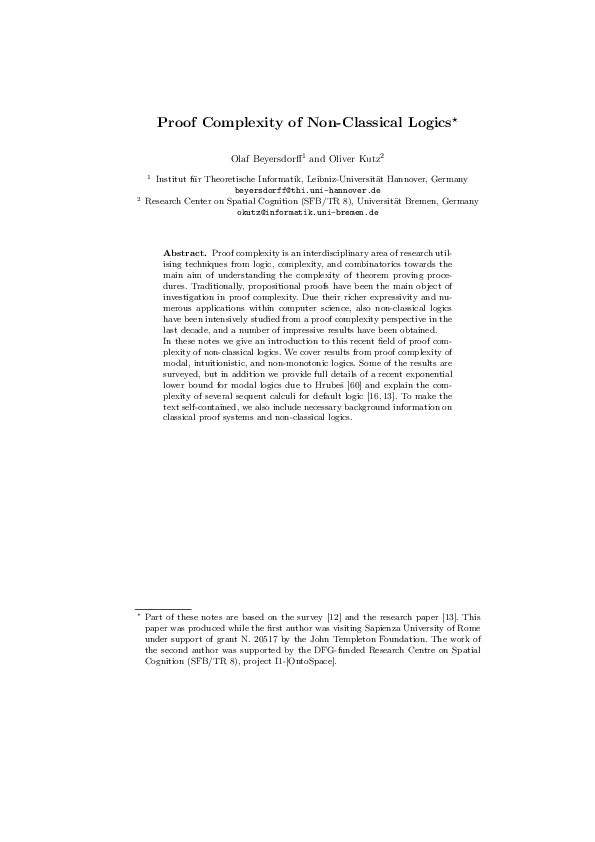
 Oliver Kutz