HYDROLOGICAL PROCESSES
Hydrol. Process. 24, 357– 367 (2010)
Published online 17 September 2009 in Wiley InterScience
(www.interscience.wiley.com) DOI: 10.1002/hyp.7457
SWAT model application and prediction uncertainty analysis
in the Lake Tana Basin, Ethiopia
Shimelis G. Setegn,1 * Ragahavan Srinivasan,2 Assefa M. Melesse3 and Bijan Dargahi1
1
Hydraulic Engineering Division, Department of Land & Water Resources Engineering, The Royal Institute of Technology (KTH), Stockholm, Sweden
2 Spatial Science Laboratory, Texas A & M University, College Station, TX, USA
3 Department of Environmental Studies, Florida International University, Miami, FL, USA
Abstract:
Lake Tana Basin is of significant importance to Ethiopia concerning water resources aspects and the ecological balance of
the area. Many years of mismanagement, wetland losses due to urban encroachment and population growth, and droughts are
causing its rapid deterioration. The main objective of this study was to assess the performance and applicability of the soil
water assessment tool (SWAT) model for prediction of streamflow in the Lake Tana Basin, so that the influence of topography,
land use, soil and climatic condition on the hydrology of Lake Tana Basin can be well examined. The physically based
SWAT model was calibrated and validated for four tributaries of Lake Tana. Sequential uncertainty fitting (SUFI-2), parameter
solution (ParaSol) and generalized likelihood uncertainty estimation (GLUE) calibration and uncertainty analysis methods
were compared and used for the set-up of the SWAT model. The model evaluation statistics for streamflows prediction shows
that there is a good agreement between the measured and simulated flows that was verified by coefficients of determination
and Nash Sutcliffe efficiency greater than 0Ð5. The hydrological water balance analysis of the basin indicated that baseflow is
an important component of the total discharge within the study area that contributes more than the surface runoff. More than
60% of losses in the watershed are through evapotranspiration. Copyright 2009 John Wiley & Sons, Ltd.
KEY WORDS
SWAT; Lake Tana; hydrological modelling; SUFI-2; GLUE; ParaSol
Received 14 November 2008; Accepted 17 July 2009
INTRODUCTION
The Lake Tana Basin is one of the basins in Ethiopia
where the major problems of soil erosion, sediment transport and land degradation are not getting much attention.
The land and water resources of the basin and its ecosystem are under great pressure stemming from the rapid
growth of population, deforestation and overgrazing, soil
erosion, sediment deposition, storage capacity reduction,
drainage and water logging, flooding, pollutant transport
and over-exploitation of specific fish species. Delivery
of sediments and organic and inorganic fertilizers from
the agricultural fields to the Lake Tana can lead to high
ecosystem productivity and impact the aquatic ecosystems. No effective measures have been taken to combat
flooding, soil erosion and sedimentation problems. The
lack of decision-support tools and limitation of data at
desired scales on soil and land use, based on hydrology
and topography, and weather are factors that significantly
hinder research and development in the area. There are
different physically based hydrological models designed
and applied to simulate the rainfall runoff relationship
under different temporal and spatial dimensions. Many
of these models share a common base in their attempt to
* Correspondence to: Shimelis G. Setegn, Hydraulic Engineering Division, Department of Land & Water Resources Engineering, The Royal
Institute of Technology (KTH), Stockholm, Sweden.
E-mail: Shimelis@kth.se; melessea@fiu.edu
Copyright 2009 John Wiley & Sons, Ltd.
incorporate the heterogeneity of the watershed and spatial distribution of topography, vegetation, land use, soil
characteristics, rainfall and evaporation. The soil water
assessment tool (SWAT) model is one of the watershed
models that play a major role in analysing the impact of
land management practices on water, sediment and agricultural chemical yields in large complex watersheds. It
is widely applied in many parts of the world. A comprehensive review of SWAT model applications is given by
Gassman et al. (2007). The ability of a watershed model
to accurately predict the hydrological process is evaluated
through parameter sensitivity analysis, model calibration
and model validation. An important issue to consider in
the prediction of hydrology, sediment yield and water
quality is uncertainties in the predictions. According to
Yang et al. (2008) the main sources of uncertainties are:
1. simplifications in the conceptual model. For example,
the simplifications in a hydrological model, or the
assumptions in the equations for estimating surface
erosion and sediment yield,
2. processes occurring in the watershed but not included
in the model. For example, wind erosion, soil losses
caused by landslides,
3. processes that are included in the model, but their
occurrences in the watershed are unknown to the modeller or unaccountable; for example, reservoirs, water
diversions, irrigation, or farm management affecting
water quality,
�358
S. G. SETEGN ET AL.
4. processes that are not known to the modeller and not
included in the model. These include dumping of waste
material and chemicals in the rivers, or processes that
may last for a number of years and drastically change
the hydrology or water quality such as constructions
of roads, bridges, tunnels and dams, and
5. errors in the input variables such as rainfall and
temperature.
The use of several calibration and uncertainty analysis
techniques are common among researchers (e.g. Eckhardt
and Arnold, 2001; Abbaspour et al., 2004; Abbaspour,
2005; Yang et al., 2007, 2008). In this study, the application of sequential uncertainty fitting (SUFI-2), parameter solution (ParaSol), generalized likelihood uncertainty
estimation (GLUE) calibration and uncertainty algorithms
is discussed.
Different hydrological studies have been conducted
in the area using different methods (e.g. Conway and
Hulme, 1993, 1996; Johnson and Curtis, 1994; Conway,
2000; Kebede et al., 2005). In this study, we focus on
calibration, evaluation and application of SWAT model
for simulation of the hydrology of Lake Tana Basin.
Hence, the main objective of this study was to test the
performance and applicability of the SWAT model for
prediction of streamflow in the Lake Tana Basin.
There are a few applications of SWAT model to
Ethiopian conditions in relatively small watershed areas
(e.g. Chekol, 2006; Setegn et al., 2007; Tadele and
Foerech 2007). The present study considers large scale
application of the model on a catchment area where
most of the topographic features have slopes greater
than 5%. For estimation of curve number to slopes
above 5%, an equation developed by Williams (1995)
was used. The ultimate goal of the study is to set up
the SWAT model for Ethiopian condition and assess its
predictive performance using different calibration and
uncertainty analysis methods and examine the influence
of topography, land use, soil and climatic condition on
the hydrological water balance of the Lake Tana Basin,
Ethiopia.
STUDY AREA
Lake Tana basin comprises a total area of 15 096 km2
including the lake area. The mean annual rainfall of
the catchment area is about 1280 mm. The annual mean
actual evapotranspiration and water yield of the catchment area are estimated to be 773 mm and 392 mm,
respectively (Setegn et al., 2008b). It is rich in biodiversity with many endemic plant species and cattle breeds;
it contains large areas of wetlands; it is home to many
endemic birds, and cultural and archaeological sites. This
basin is of critical national significance as it has great
potentials for irrigation, hydroelectric power, high value
crops and livestock production, ecotourism and others.
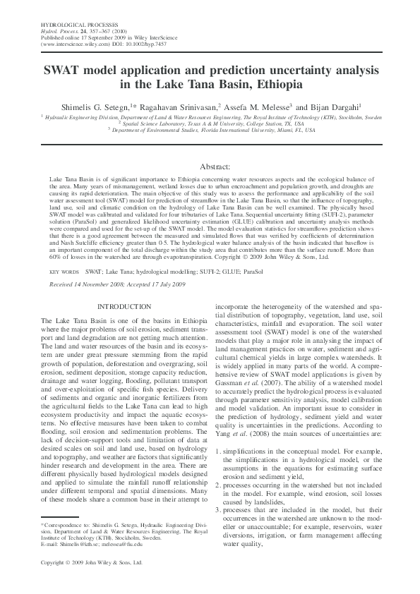
Lake Tana is located in the country’s north-west highlands (Lat 12° 00 N, Lon 37° 150 E) (Figure 1). The lake is
a natural type which covers 3000–3600 km2 area at an
elevation of 1800 m and with a maximum depth of 15 m.
It is approximately 84 km long, 66 km wide. It is the
largest lake in Ethiopia and the third largest in the Nile
Basin. Gilgel Abay, Ribb, Gumera and Megech are the
main rivers feeding the lake, which contributes more than
90% of the inflow. It is the main source of the Blue Nile
river, which is the only surface outflow for the Lake. The
climate of the region is ‘tropical highland monsoon’ with
the main rainy season between June and September. The
air temperature shows large diurnal but small seasonal
changes with an annual average of 20 ° C.
METHODS
The present study discusses the application of a physically based watershed model, SWAT, in the Lake Tana
Basin. The application of the model involved calibration,
sensitivity and uncertainty analysis. For this purpose,
SUFI-2, ParaSol and GLUE calibration and uncertainty
analysis algorithms were used.
Description of soil and water assessment tool (SWAT)
SWAT is a public domain model developed by Arnold
et al. (1998). It is a spatially distributed, continuous river
Figure 1. Location map of the study area
Copyright 2009 John Wiley & Sons, Ltd.
Hydrol. Process. 24, 357–367 (2010)
DOI: 10.1002/hyp
�SWAT MODEL APPLICATION AND PREDICTION UNCERTAINTY ANALYSIS
basin scale model developed to predict the impact of
land management practices on water, sediment and agricultural chemical yields in large complex watersheds
with varying soils, land use and management conditions
over long periods of time (Neitsch et al., 2005). SWAT
uses hydrological response units (HRUs) to describe spatial heterogeneity in terms of land cover, soil type and
slope within a watershed. The SWAT system is embedded
within geographic information system (GIS) that can integrate various spatial environmental data including soil,
land cover, climate and topographic features. Currently,
SWAT is embedded in an ArcGIS interface called ArcSWAT. The simulation of the hydrology of a watershed
is done in two separate divisions. One is the land phase
of the hydrological cycle that controls the amount of
water, sediment, nutrient and pesticide loadings to the
main channel in each subbasin. The other division is
the routing phase of the hydrological cycle that can be
defined as the movement of water, sediments, nutrients
and organic chemicals through the channel network of the
watershed to the outlet. In the land phase of hydrological
cycle, SWAT simulates the hydrological cycle based on
the water balance equation.
SWt D SW0 C
t
�
�
�
Rday � Qsurf � Ea � wseep � Qqw i
iD1
⊲1⊳
in which SWt is the final soil water content (mm), SWo
is the initial soil water content on day i (mm), t is the
time (days), Rday is the amount of precipitation on day
i (mm), Qsurf is the amount of surface runoff on day i
(mm), Ea is the amount of evapotranspiration on day i
(mm), Wseep is the amount of water entering the vadose
zone from the soil profile on day i (mm) and Qgw is
the amount of return flow on day i (mm).SWAT offers
two methods for estimating surface runoff: the SCS curve
number procedure (USDA-SCS, 1972) and the Green and
Ampt infiltration method (Green and Ampt, 1911). In this
study, the SCS curve number method was used to estimate the surface runoff. SWAT 2005 version includes
two methods for calculating the retention parameter. In
the first one, the retention parameter varies with soil profile water content. This method overestimates runoff in
shallow soils. In the second method, the retention parameter varies with accumulated plant evapotranspiration.
Calculating daily curve number (CN) as a function of
plant evapotranspiration is more dependant on antecedent
climate. SWAT calculates the peak runoff rate with a
modified rational method. Three methods are incorporated into SWAT to estimate potential evapotranspiration
(PET): the Penman–Monteith method (Monteith, 1965),
the Priestley–Taylor method (Priestley and Taylor, 1972)
and the Hargreaves method (Hargreaves et al., 1985).
For this study, we have used Hargreaves method. The
simulation of groundwater is partitioned into two aquifer
systems, i.e. an unconfined aquifer (shallow) and a deepconfined aquifer in each subbasin. The unconfined aquifer
contributes to flow in the main channel or reach of the
subbasin. Water that enters the deep aquifer is assumed to
Copyright 2009 John Wiley & Sons, Ltd.
359
contribute to stream flow outside the watershed (Arnold
et al., 1993). In SWAT, the water balance for a shallow
aquifer is calculated with Equation (2):
aqsh,i D aqsh,i�1 C wrchrg � Qgw � wrevap � wdeep
� wpump,sh
⊲2⊳
in which aqsh,i is the amount of water stored in the
shallow aquifer on day i (mm), aqsh,i�1 is the amount of
water stored in the shallow aquifer on day i � 1 (mm),
wrchrg is the amount of recharge entering the aquifer on
day i (mm), Qgw is the groundwater flow, or base flow,
into the main channel on day i (mm), wrevap is the amount
of water moving into the soil zone in response to water
deficiencies on day i (mm), wdeep is the amount of water
percolating from the shallow aquifer into the deep aquifer
on day i (mm) and wpump,sh is the amount of water
removed from the shallow aquifer by pumping on day
i (mm).
The steady-state response of groundwater flow to
recharge is estimated by Hooghoudt equation
(Hooghoudt, 1940). In SWAT, water is routed though the
channels network using either the variable storage routing or Muskingum River routing method. More detailed
descriptions of the different model components are listed
in Arnold et al. (1998) and Neitsch et al. (2005).
SWAT model input
Digital elevation model (DEM). A 90 by 90 m2 resolution DEM was downloaded from the shuttle radar
topography mission (SRTM) website (Jarvis et al., 2006).
The DEM was used to delineate the watershed and to
analyse the drainage patterns of the land surface terrain.
Subbasin parameters such as slope gradient, slope length
of the terrain, and the stream network characteristics such
as channel slope, length and width were derived from
the DEM.
Soil data. SWAT model requires different soil textural and physico-chemical properties such as soil texture, available water content, hydraulic conductivity, bulk
density and organic carbon content for different layers of each soil type. The soil data is obtained mainly
from the following sources: Soil and Terrain Database
for north-eastern Africa CD-ROM (Food and Agriculture Organization of the United Nations FAO (1998),
Major Soils of the world CD-ROM FAO (2002), Digital Soil Map of the World and Derived Soil Properties CD-ROM FAO (1995), Properties and Management of Soils of the Tropics CD-ROM Van Wambeke
(2003), Abbay river basin Integrated Development Master Plan Project—Semi detailed Soil Survey and the
Soils of Anjeni Area, Ethiopia (SCRP, 2000). These
sources were utilized to extract the necessary soil properties in relation to the major soil type map developed
by Ethiopian ministry of water resources. The different
sources have helped in correlating and verification of the
soil properties. Major soil types in the basin are Chromic
Hydrol. Process. 24, 357– 367 (2010)
DOI: 10.1002/hyp
�360
S. G. SETEGN ET AL.
Figure 2. Soil and Land use/land cover map of Lake Tana Basin
Figure 3. Weather and streamflow gauge stations, subbasins and river layers in Lake Tana Basin
Luvisols, Eutric Cambisols, Eutric Fluvisols, Eutric Leptosols, Eutric Regosols, Eutric Vertisols, Haplic Alisols,
Haplic Luvisols, Haplic Nitisols and Lithic Leptosols
(Figure 2a).
Land use. Land use is one of the most important factors
that affect runoff, evapotranspiration and surface erosion
in a watershed. The land use map of the study area
was obtained from ministry of water resources Ethiopia
and Soil Conservation Research Programme (SCRP),
University of Bern, Switzerland. The land use of the area
was reclassified based on the available topographic map
(1 : 50 000), aerial photographs, satellite images and field
data. The reclassification of the land use map was done
to represent the land use according to the specific land
cover types. The main land cover types of the area are
cultivated land, lake water surface, pasture, forest and
wetland. Figure 2b shows that more than 50% of the Lake
Tana Basin is cultivated land mainly for Teff, maize and
barley crops.
Weather data. In this study, the weather variables used
for driving the hydrological balance are daily precipitation, minimum and maximum air temperature for the
period 1978–2004. The data is obtained from Ethiopian
Copyright 2009 John Wiley & Sons, Ltd.
National Meteorological Agency (NMA) for stations
located within and around the watershed (Figure 3).
River discharge and sediment yield . Daily river discharge values for Ribb, Gumera, Gilgel Abay, Megech
rivers and the outflow river Blue Nile (Abbay) were
obtained from the Hydrology Department of the Ministry of Water Resources of Ethiopia (Figure 3). These
daily river discharges data were used for model calibration (1981–1992) and validation (1993–2004). Figure 4
shows that the peak flows for all inflow rivers are in
August. But the outflow river gets its peak flow during
the month of September. There is a one month delay of
peak flow for the outflow river. This is due to the influence of the lake that retards the flow before it reaches
the outlet.
Model set-up
The model set-up involved five steps: (1) data preparation, (2) subbasin discretization, (3) HRU definition,
(4) parameter sensitivity analysis and (5) calibration and
uncertainty analysis. A predefined digital stream network
layer was imported and superimposed onto the DEM to
accurately delineate the location of the streams. The land
use/land cover spatial data were reclassified into SWAT
Hydrol. Process. 24, 357–367 (2010)
DOI: 10.1002/hyp
�SWAT MODEL APPLICATION AND PREDICTION UNCERTAINTY ANALYSIS
361
Figure 4. Average monthly flows for the major tributary rivers of Lake Tana and outflow river
land cover/plant types. The watershed delineation process
include five major steps, DEM set-up, stream definition,
outlet and inlet definition, watershed outlets selection and
definition and calculation of subbasin parameters. For
the stream definition, the threshold-based stream definition option was used to define the minimum size of
the subbasin. The land use, soil and slope datasets were
imported, overlaid and linked with the SWAT databases.
Subdividing the sub watershed into hydrological response
units (HRU’s), which are areas having unique land use,
soil and slope combinations makes it possible to study the
differences in evapotranspiration and other hydrological
conditions for different land covers, soils and slopes.
Model calibration and evaluation
Twenty six hydrological parameters were tested for
sensitivity analysis for the simulation of the stream
flow in the study area. The details of all hydrological
parameters are found in Winchell et al. (2007). The data
for period 1981–1992 were used for calibration and from
1993 to 2004 were used for validation of the model in the
four tributaries of Lake Tana basin. Periods 1978–1980
and 1990–1992 were used as ‘warm-up’ periods for
calibration and validation purposes, respectively. The
warm-up period allows the model to get the hydrological
cycle fully operational.
The calibration and uncertainty analysis were done
using three different algorithms, i.e. SUFI-2 (Abbaspour
et al., 2004, 2007), ParaSol (Van Griensven and Meixner,
2006) and GLUE (Beven and Binley, 1992). These
methods are chosen for their applicability from simple
to complex hydrological models.
Sequential uncertainty fitting—SUFI-2 . SUFI-2 is the
calibration algorithm developed by Abbaspour et al.
(2004, 2007) for the calibration of SWAT model. In
SUFI-2, parameter uncertainty accounts for all sources of
uncertainties such as uncertainty in driving variables (e.g.
rainfall), parameters, conceptual model and measured
data (e.g. observed flow, sediment). In SUFI-2, the
degree to which all uncertainties are accounted for is
quantified by a measure referred to as the p-factor,
which is the percentage of measured data bracketed by
the 95% prediction uncertainty (95PPU). The 95PPU is
calculated at the 2Ð5% and 97Ð5% levels of the cumulative
distribution of an output variable obtained through Latin
Copyright 2009 John Wiley & Sons, Ltd.
hypercube sampling. Latin hypercube sampling is used
to draw independent parameter sets (Abbaspour et al.,
2007). Another measure quantifying the strength of a
calibration/uncertainty analysis is the so called r-factor,
which is the average thickness of the 95PPU band
(r) divided by the standard deviation of the measured
data. When acceptable values of r-factor and p-factor
are reached, the parameter uncertainties are the desired
parameter ranges. The SUFI-2 analysis consists of the
following procedures (Yang et al., 2008):
1. In the first step, the objective function (OF) g⊲�⊳ and
meaningful parameter ranges (�abs min, �abs max) are
defined.
2. Then a Latin Hypercube sampling is carried out in
the hypercube (�min, �max) [initially set to (�abs min,
�abs max)], the corresponding OFs are evaluated, and
the sensitivity matrix J and the parameter covariance
matrix C are calculated according to:
Jij D
gi
i D 1, . . . , C2 m , j D 1, . . . , n,
�j
C D Sg 2 ⊲JT J⊳�1
⊲3⊳
⊲4⊳
where Sg 2 is the variance of the OF values resulting from
the m model runs.
3. A 95% predictive interval of a parameter �j is computed as follows:
�
�j,lower D �jŁ � tv,0�025 Cjj , �j,upper
�
D �jŁ � tv,0Ð025 Cjj
⊲5⊳
Where �jŁ is the parameter �j for the best estimates
(i.e. parameters which produce the optimalOF), and � is
the degrees of freedom (m –n).
4. The 95PPU is calculated. And then two indices, i.e.
the p-factor (the percent of observations bracketed by
the 95PPU) and the r-factor. The average thickness of
the 95PPU band (r) and the r-factor are calculated by
Equations (6) and (7):
n
1� M
⊲yti ,97Ð5% � ytMi ,2Ð5% ⊳
rD
n t
⊲6⊳
i
r � factor D
r
�obs
⊲7⊳
Hydrol. Process. 24, 357– 367 (2010)
DOI: 10.1002/hyp
�362
S. G. SETEGN ET AL.
in which ytMi ,97Ð5% and ytMi ,2Ð5% represent the upper and
lower boundaries of the 95PPU, and �obs is the standard
deviation of the measured data.
The goodness of calibration and prediction uncertainty
is judged on the basis of the closeness of the p-factor to
100% (i.e. all observations bracketed by the prediction
uncertainty), and the r-factor to 1 (i.e. achievement of
rather small uncertainty band). According to Yang et al.
(2008) as all uncertainties in the conceptual model and
inputs are reflected in the measurements (e.g. discharge),
bracketing most of the measured data in the prediction
95PPU ensures that all uncertainties are depicted by
the parameter uncertainties. If the two factors have
satisfactory values, then a uniform distribution in the
parameter hypercube (�min , �max ) is interpreted as the
posterior parameter distribution.
Further goodness of fit can be quantified by the
coefficient of determination (R2 ), which is the percent
of the variation that can be explained by the regression
equation and Nash–Sutcliffe coefficient (NSE) between
the observations and the final best simulation.
Coefficient of determination R2 calculated as:
�2
�
��
��
�
Qm,i � Qm Qs,j � Qs
R2 D � �i
Qm,j � Qm
�2 � �
�2
Qs,i � Qs
⊲8⊳
i
i
Nash–Sutcliffe (1970) coefficient calculated as:
�
⊲Qm � Qs ⊳2i
NSE D 1 � �i
⊲Qm,i � Qm ⊳2
where, N is the number of behavioral parameter sets.
3. Finally, prediction uncertainty is described by quantiles of the cumulative distribution realized from the
weighted behavioural parameter sets. The most frequently used likelihood measure for GLUE is the NSE
[Equation (9)].
Parameter solution (ParaSol). ParaSol is an optimization and statistical uncertainty method that assesses
model parameter uncertainty (Van Griensven and
Meixner, 2006). The ParaSol method was developed to
perform optimization and model parameter uncertainty
analysis for complex distributed models, typically having
a high number of parameters, high parameter correlations,
several output variables and a complex structure leading
to multiple minima in the OF response surface. The ParaSol method calculates OFs based on model outputs and
observation time series, aggregates these OFs to a global
optimization criterion (GOC) and minimizes the OF or
a GOC using the Shuffled Complex Evolution (SCEUA) algorithm. The SCE-UA algorithm is developed by
Duan et al. (1992). It is a global search algorithm for the
minimization of a single function with up to 16 parameters (Duan et al., 1992). It minimizes the differences
between model predicted and measured flow by modifying selected SWAT model parameters. The SCE-UA has
been applied with success on SWAT for the hydrological
parameters (Eckardt and Arnold, 2001), and hydrological and water quality parameters (van Griensven and
Bauwens, 2003).
The OF used in ParaSol is Sum of the squares of the
residuals (SSQ):
⊲9⊳
SSQ D
i
n
�
⊲ytMi ⊲�⊳ � yti ⊳2
⊲11⊳
ti �1
Generalized likelihood uncertainty estimation—glue.
The GLUE (Beven and Binley, 1992) was introduced
partly to allow for the possible non-uniqueness of parameter sets during the estimation of model parameters in
over-parameterized models. It is an uncertainty technique
inspired by importance sampling and regional sensitivity
analysis (Hornberger and Spear, 1981). Similar to SUGI2, GLUE accounts for all sources of uncertainties.
The GLUE analysis consists of the following procedures (Yang et al., 2008).
The relationship between NSE and SSQ can be stated
as:
1
Ð SSQ
⊲12⊳
NSE D 1 � n
�
2
⊲yti � y⊳
1. After the definition of the ‘generalized likelihood
measure’, L⊲�⊳, a large number of parameter sets are
randomly sampled from the prior distribution, and each
parameter set is assessed as either ‘behavioral’ or ‘nonbehavioral’ through a comparison of the ‘likelihood
measure’ with a selected threshold value.
2. Each behavioral parameter set is given a ‘likelihood
weight’ according to
RESULTS AND DISCUSSION
wi D
L⊲�i ⊳
N
�
L⊲�k ⊳
kD1
Copyright 2009 John Wiley & Sons, Ltd.
⊲10⊳
ti D1
�n
where ti D1 ⊲yti � y⊳2 is a fixed value for given observations, and NSE and SSQ have the one-to-one relation
ship.
Parameter sensitivity analysis
The parameter sensitivity analysis was done using the
ArcSWAT interface for the whole catchment area. Twenty
six hydrological parameters were tested for sensitivity
analysis for the simulation of the stream flow in the
study area. The most sensitive parameters considered for
calibration were soil evaporation compensation factor,
initial SCS Curve Number II value, base flow alpha factor
(days), threshold depth of water in the shallow aquifer for
‘revap’ to occur (mm), (days), available water capacity
Hydrol. Process. 24, 357–367 (2010)
DOI: 10.1002/hyp
�363
SWAT MODEL APPLICATION AND PREDICTION UNCERTAINTY ANALYSIS
Table I. SWAT flow sensitive parameters and fitted values after
calibration using SUFI-2
Final fitted value
Sensitive
parameters
1
2
3
4
5
6
7
8
Lower and Gilgel Megech
Upper
Abay
river
bound
river
ESCO
CN2
ALPHA BF
REVAPMN
SOL AWC
GW REVAP
CH K2
GWQMN
0–1
š25%
0–1
0–500
š25%
š0Ð036
0–5
0–5000
0Ð8
�10%
0Ð1
300
20%
0Ð04
4Ð6
108
0Ð8
�9%
0Ð1
289
�20%
0Ð1
3Ð2
17
Ribb
river
Gumera
river
0Ð8
�10%
0Ð1
372
�10%
0Ð04
1Ð9
333
0Ð8
�8
0Ð1
446
20%
0Ð1
0Ð7
98
(mm WATER/mm soil), groundwater ‘revap’ coefficient,
channel effective hydraulic conductivity (mm/h) and
threshold depth of water in the shallow aquifer for return
flow to occur (mm) Table I describes the most sensitive
flow parameters and their fitted values.
Model calibration and validation
SUFI-2, GLUE and ParaSol methods were used for
calibration of the SWAT model in Gilgel Abay, Gumera,
Ribb and Megech inflow rivers. The comparison between
the observed and simulated streamflow indicated that
there is a good agreement between the observed and
simulated discharge which was verified by higher values of coefficient of determination (R2 ) and NSE. In
Megech river, the predictive performance of the model
is poor both during the calibration and validation period
(Table II). Calibrated and validated model predictive performances for all rivers on daily flows are summarized
in Table II for all calibration and uncertainty analysis
methods.
SUFI-2 method: The SUFI-2 results indicated that
the p-factor which is the percentage of observations
bracketed by the 95% prediction uncertainty (95PPU),
brackets 82% of the observation and r-factor equals 0Ð80
for Gilgel Abay river. The 95PPU brackets only 53% of
the observations, and r-factor equals to 0Ð39 for Megech
river during calibration period. For Gumera and Ribb
rivers 79 and 73% of observed flow data was bracketed by
95PPU. Furthermore, 79% of the observed data bracketed
by 95PPU for Gilgel Abay river, 73% for Gumera, 65%
for Ribb and 57% for Megech rivers during the validation
period.
GLUE method: In GLUE method, the p-factor brackets 76% of the observation, and r-factor equals 0Ð65 for
Gilgel Abay river. The 95PPU brackets only 55% of the
observations and r-factor equals to 0Ð11 for Megech river
during calibration period. For Gumera and Ribb rivers, 73
and 66% of observed flow data were bracketed by 95PPU.
Furthermore, 75% of the observed data was bracketed by
95PPU for Gilgel Abay river, 64% for Gumera, 61% for
Ribb and 46% for Megech rivers during the validation
period.
ParaSol method: In this method, the p-factor brackets
21% of the observation and r-factor equals 0Ð10 for
Gilgel Abay river. The 95PPU brackets only 15% of the
observations, and r-factor equals to 0Ð02 for Megech river
during calibration period. For Gumera and Ribb rivers 19
and 17% of observed flow data were bracketed by 95PPU.
Furthermore, 19% of the observed data was bracketed by
95PPU for Gilgel Abay river, 17% for Gumera, 16% for
Ribb and 15% for Megech rivers during the validation
period.
The analysis shows that the SUFI-2 did not capture the
observations well during calibration period for Megech
river. This problem coupled with the lower values of NSE
and R2 for Megech river indicates that there is uncertainty
in simulated flow due to errors in input data such as rainfall and temperature, and/or other sources of uncertainties such as upstream dam constructions for town water
supply, which have a reservoir capacity of 5Ð3 million
m3 , diversion of streams for small scale irrigation and
Table II. Stream flow calibration and validation results for Gilgel Abay, Gumera, Megech and Ribb rivers using SUFI-2, GLUE and
ParaSol methods
Objective function
Rivers
Gilgel Abay
NSE
R2
p-factor
r-factor
SUFI-2
GLUE
PARASOL
SUFI-2
GLUE
PARASOL
SUFI-2
GLUE
PARASOL
SUFI-2
GLUE
PARASOL
Gumera
Megech
Ribb
Cal
Val
Cal
Val
Cal
Val
Cal
Val
0Ð73
0Ð58
0Ð73
0Ð75
0Ð79
0Ð80
83%
76%
21%
0Ð81
0Ð65
0Ð10
0Ð69
0Ð69
0Ð71
0Ð80
0Ð80
0Ð78
79%
75%
19%
0Ð77
0Ð69
0Ð08
0Ð62
0Ð60
0Ð61
0Ð69
0Ð71
0Ð71
79%
73%
19%
0Ð75
0Ð62
0Ð08
0Ð60
0Ð60
0Ð61
0Ð70
0Ð70
0Ð70
73%
64%
17%
0Ð72
0Ð65
0Ð05
0Ð18
0Ð20
0Ð22
0Ð19
0Ð25
0Ð20
53%
55%
15%
0Ð39
0Ð11
0Ð02
0Ð04
0Ð04
0Ð20
0Ð32
0Ð32
0Ð31
57%
46%
15%
0Ð33
0Ð13
0Ð02
0Ð51
0Ð50
0Ð55
0Ð59
0Ð58
0Ð59
73%
66%
17%
0Ð58
0Ð45
0Ð06
0Ð48
0Ð48
0Ð45
0Ð55
0Ð55
0Ð57
65%
61%
16%
0Ð54
0Ð49
0Ð05
Cal, Calibration; Val, Validation.
Copyright 2009 John Wiley & Sons, Ltd.
Hydrol. Process. 24, 357– 367 (2010)
DOI: 10.1002/hyp
�364
S. G. SETEGN ET AL.
other unknown activities in the subbasins. The study also
used the Hargreaves method (Hargreaves et al., 1985) to
calculate evapotranspiration that depends on minimum
and maximum temperatures. Hargreaves method does not
include the effect of wind on evapotranspiration. In cases
where the wind is a predominating factor, the method can
introduce some errors. Hence, in the study area the wind
speed ranges from 3 to 6 m/s which may have a significant influence on the loss of water by evapotranspiration.
The lack of meteorological data did not allow it
to consider additional factors. We have assumed that
the model deficiency in Megech watershed could be
due to the input uncertainties as well as construction
of infrastructures in the upstream of the watershed.
However, we cannot rule out the possibility of an error in
the type of soil and the corresponding soil properties in
the area. This can cause some uncertainty in the simulated
results. Another issue is the soil erosion that affects the
structure, infililtration capacity and other properties of
the soil. As the model does not consider the effect of soil
erosion on runoff, the predictions can be uncertain.
The calibration process using SUFI-2 algorithm gave
the final fitted parameters for each river basin (Table I).
The final values for CN2, Soil AWC include the amount
adjusted during the manual calibration. These parameters
were incorporated into the SWAT model for validation
and further applications. The validation result was good
for Gilgel Abay, Gumera and Ribb rivers with high
values of R2 and NSE (Table II). Time series of measured
and simulated daily flows with respect to the depth of
Figure 5. Time series of measured and simulated daily flow validation results at Gilgel Abay river gauge station
Copyright 2009 John Wiley & Sons, Ltd.
Hydrol. Process. 24, 357–367 (2010)
DOI: 10.1002/hyp
�SWAT MODEL APPLICATION AND PREDICTION UNCERTAINTY ANALYSIS
Figure 6. A scattergram comparison between measures and simulated
daily flow for calibration period at Gilgel Abay river gauge station
rainfall in Gilgel Abay river basin indicated that both
the observed and simulated flow discharge follow the
rainfall pattern of the area. The higher discharge occurs
during the months of June to September. This high
flow corresponds to the longer rainy season. Above 75%
of annual flow occurs in this period. Figure 5 and 6
show the time series comparison between measured and
simulated daily flow at Gilgel Abay river gauge station
during calibration period.
Hydrological water balance
The baseflows were evaluated on an annual basis for
Gilgel Abay, Gumera, Megech and Ribb river basins.
The baseflow filter program by Arnold and Allen (1999)
generates a range of predicted baseflow volumes. On an
annual basis, the measured flow at Gilgel Abay river
gauge station is estimated as 59% baseflow over the
calibration period. In comparison, the simulated flow
at Gilgel Abay is estimated as 54% baseflow over
the calibration period. Therefore, the calibrated model
365
was considered to generate acceptable predictions of
baseflow. Figure 7 shows the time series graph showing
baseflow separated from observed and simulated flow for
Gilgel Abay river.
The main water balance components of the four river
basins include: the total amount of precipitation falling
on the subbasin during the time step, actual evapotranspiration from the basin and the net amount of water
that leaves the basin and contributes to streamflow in
the reach (water yield). The water yield includes surface
runoff contribution to streamflow, lateral flow contribution to streamflow (water flowing laterally within the soil
profile that enters the main channel), groundwater contribution to streamflow (water from the shallow aquifer
that returns to the reach) minus the transmission losses
(water lost from tributary channels in the HRU via transmission through the bed and becomes recharge for the
shallow aquifer during the time step). Table III lists the
simulated water balance components on an annual average basis for the Lake Tana Basin over the calibration and
validation period. The results indicated that 65% of the
annual precipitation is lost by evapotranspiration in the
basin during calibration as compared to 56% during validation period. Surface runoff contributes 31 and 25% of
the water yield during calibration and validation period,
respectively, whereas the groundwater contributes 45 and
54% of the water yield during calibration and validation
period, respectively.
The annual average rainfall and other hydrological
components were compared for each year of the calibration and validation periods for Gilgel Abay river. The
year 1982 was a dry year and 1991 was a wet year for
calibration period, and 1994 and 2003 were the driest
and the wettest years, respectively, during the validation period for Gilgel Abay river. The use of the term
‘dry’ is relative as the rainfall is greater than 900 mm.
The wet years produce a larger water yield than the dry
years. The water fluxes in the basin indicate that in a
wet year surface runoff dominates water yield, which is
the total amount of water leaving the HRU and entering
main channel during the time step. However, in a dry
year, lateral flow contribution makes up a larger part of
the water yield. As indicated in Figure 8, in a dry year the
Figure 7. Time series graph showing Baseflow separated from observed and simulated flow for Gilgel Abay river
Copyright 2009 John Wiley & Sons, Ltd.
Hydrol. Process. 24, 357– 367 (2010)
DOI: 10.1002/hyp
�366
S. G. SETEGN ET AL.
Table III. Water balance components on an annual average basis over the calibration and validation periods for the Lake Tana Basin
Period
Calibration
Validation
(mm)
(%)
(mm)
(%)
Rainfall
ET
SurQ
LatQ
GW Q
WYLD
SW
PERC
TLOSS
1168
100Ð0
1394
100Ð0
758
64Ð9
782
56Ð1
95
8Ð1
120
8Ð6
73
6Ð2
101
7Ð2
137
11Ð7
254
18Ð2
305
26Ð1
474
34Ð0
217
18Ð6
227
16Ð3
251
21Ð5
400
28Ð7
12
1Ð0
13
1Ð0
ET, Actual Evapotranspiration from HRU; SW, Soil water content; PERC, water that percolates past the root zone during the time step; SURQ, Surface
runoff contribution to streamflow during time step; TLOSS, Transmisson losses—water lost from tributary channels in the HRU via transmission
through the bed; GW Q, Ground water contribution to streamflow; LAT Q, Lateral floe contribution to streamflow; WYLD, water yield (water yield
D SURQCLATQCGWQ-TLOSS-pond abstractions).
Figure 8. Low flow (top) and high flow (middle) condition in Gilgel Abay river for validation period
simulated streamflow is lower than the observed flow. It
resulted is some degree of prediction uncertainties. However, in wet year condition the simulated flow fits the
observed stream flow. This indicates that the model efficiency differs between wet and dry year conditions in
the study area. Based on the above result, we can assume
that the model can better predict the surface runoff than
the groundwater contribution to stream flow during the
wet season. One reason could be due to the soil data
quality and estimation of the curve number at dry moisture condition. As the SCS curve number is a function
of the soil’s permeability, land use and antecedent soil
water conditions, the estimation of curve number at dry
moisture condition (wilting point) might not be efficient
in that watershed.
CONCLUSION
Land and water resources degradation are the major problems on the Ethiopian highlands. Poor land use practices
and improper management systems have a significant
role in causing high soil erosion rates, sediment transport
and loss of agricultural nutrients. The SWAT model was
applied to the Lake Tana Basin for the modelling of the
hydrological water balance. It was successfully calibrated
and validated for the four main tributaries of Lake Tana.
The model evaluation statistics for streamflows gave good
Copyright 2009 John Wiley & Sons, Ltd.
results that were verified by NSE and R2 > 0Ð50. SUFI-2,
GLUE and ParaSol algorithms gave good results in minimizing the differences between observed and simulated
streamflows. The p-factor and r-factor computed using
SUFI-2 and GLUE gave good results by bracketing more
than 60% of the observed data. A SUFI-2 algorithm is
an effective method, but it requires additional iterations
as well as the need for the adjustment of the parameter
ranges. The hydrological water balance analysis showed
that baseflow is an important component of the total
discharge within the study area that contributes more
than the surface runoff. More than 60% of losses in the
watershed are through evapotranspiration. Despite different source of uncertainties, the SWAT model produced
good simulation results for daily and monthly time steps.
The study has shown that the SWAT model can produce reliable estimates of the different components of
hydrological cycle. The calibrated model can be used
for further analysis of the effect of climate and land use
changes, as well as to investigate the effect of different management scenarios on streamflows and sediment
yields.
REFERENCES
Abbaspour KC. 2005. Calibration of hydrologic models: when is a model
calibrated? In MODSIM 2005 International Congress on Modelling and
Simulation, Zerger A, Argent RM (eds). Modelling and Simulation
Hydrol. Process. 24, 357–367 (2010)
DOI: 10.1002/hyp
�SWAT MODEL APPLICATION AND PREDICTION UNCERTAINTY ANALYSIS
Society of Australia and New Zealand; 2449– 12455, December, ISBN:
0-9758400-2-9.
Abbaspour KC, Johnson CA, Van Genuchten MT. 2004. Estimating
uncertain flow and transport parameters using a sequential uncertainty
fitting procedure. Vadose Zone Journal 3(4): 1340– 1352.
Abbaspour KC, Yang J, Maximov I, Siber R, Bogner K, Mieleitner J,
Zobrist J, Srinivasan R. 2007. Modelling hydrology and water quality
in the pre-alpine/alpine Thur watershed using SWAT. Journal of
Hydrology 333: 413– 430.
Arnold JG, Allen PM. 1999. Automated methods for estimating baseflow
and ground water recharge from streamflow records. Journal of
American Water Resources Association 35(2): 411–424.
Arnold JG, Allen PM, Bernhardt G. 1993. A comprehensive surface
groundwater flow model. Journal of Hydrology 142: 47–69.
Arnold JG, Srinivasan R, Muttiah RR, Williams JR. 1998. Large area
hydrologic modeling and assessment part i: model development.
Journal of the American Water Resources Association 34(1): 73–89.
Beven K, Binley A. 1992. The future of distributed models: model
calibration and uncertainty prediction. Hydrological Processes 6:
279– 298.
Chekol DA. 2006. Modeling of Hydrology and Soil Erosion in Upper
Awash River Basin. University of Bonn, Institut für Städtebau,
Bodenordnung und Kulturtechnik 2006. 235pp.
Conway D. 2000. The climate and hydrology of the Upper Blue Nile
river. The Geographical Journal 166: 49–62.
Conway D Hulme M. 1993. Recent fluctuations in precipitation and
runoff over the Nile sub basins and their impact on the main Nile
discharge. Climate Change 25: 127–151.
Conway D, Hulme M. 1996. The impacts of climate variability and future
climate change in the Nile basin on water resources in Egypt. Water
Resources Development 12: 261–280.
Duan QY, Sorooshian S, Gupta V. 1992. Effective and efficient global
optimization for conceptual rainfall-runoff models. Water Resources
Research 28(4): 1015– 1031.
Eckhardt K, Arnold J. 2001. Automatic calibration of a distributed
catchment model. Journal of Hydrology 251: 103– 109.
Eckhardt K, Arnold JG. 2001. Automatic calibration of a distributed
catchment model. Journal of Hydrology 251: 103– 109.
FAO. 2002. Major Soils of the World . Land and Water Digital Media
Series Food and Agricultural Organization of the United Nations:
Rome, CD-ROM.
FAO. 1995. Digital Soil Map of the World and Derived Soil Properties
(CDROM) Food and Agriculture Organization of the United Nations.
FAO Rome, Italy.
FAO. 1998. The Soil and Terrain Database for northeastern Africa
(CDROM). FAO: Rome.
Gassman PW, Reyes MR, Green CH, Arnold JG. 2007. The soil and
water assessment tool: historical development, applications, and future
research directions. Transactions of the ASABE 50(4): 1211– 1250.
Green WH, Ampt GA. 1911. Studies on soil physics, 1. The flow of air
and water through soils. Journal of Agricultural Sciences 4: 11–24.
Hargreaves GL, Hargreaves GH, Riley JP. 1985. Agricultural benefits for
Senegal River basin. Journal of Irrigation and Drainage Engineering
111(2): 113–124.
Hooghoudt SB. 1940. Bijdrage tot de kennis van enige natuurkundige
grootheden van de grond. Verslagen van Landbouwkundige Onderzoekingen 46: 515– 707.
Hornberger GM, Spear RC. 1981. An approach to the preliminary
analysis of environmental systems. Journal of Environmental
management 12(1): 7–18.
Jarvis A, Reuter HI, Nelson A, Guevara E. 2006. Hole-filled seamless
SRTM data V3, International Centre for Tropical Agriculture (CIAT),
20 September 2007, available from http://srtm.csi.cgiar.org.
Johnson PA, Curtis PD. 1994. Water Balance of Blue Nile River Basin
in Ethiopia. Journal of Irrigation and Drainage Engineering 120:
573– 589.
Copyright 2009 John Wiley & Sons, Ltd.
367
Kebede S, Travi Y, Alemayehu T, Marc V. 2005. Water balance of Lake
Tana and its sensitivity to fluctuations in rainfall, Blue Nile Basin,
Ethiopia. Journal of Hydrology 316(1– 4): 233–247.
Monteith JL. 1965. Evaporation and the environment. In The State
and Movement of Water in Living Organisims, XIXth Symposium on
the Society of Experimental Biology. Cambridge University Press:
Swansea; 205– 234.
Nash JE, Sutcliffe JV. 1970. River flow forecasting through conceptual
models. Part I–A discussion of principles. Journal of Hydrology 10:
282– 290.
Neitsch SL, Arnold JG, Kiniry JR, Williams JR. 2005. Soil and
Water Assessment Tool, Theoretical Documentation: Version. USDA
Agricultural Research Service and Texas A &M Blackland Research
Center: Temple, TX.
Priestley CHB, Taylor RJ. 1972. On the assessment of surface heat flux
and evaporation using large-scale parameters. Monthly Weather Review
100: 81–92.
SCRP (Soil Conservation Research Program). 2000. Soil Erosion and
Conservation Database. Area of Anjeni, Gojam, Ethiopia: LongTerm Monitoring of the Agricultural Environment, 1984– 1994. Berne,
Switzerland: Centre for Development and Environment in association
with the Ministry of Agriculture, Ethiopia.
Setegn SG, Dargahi B, Srinivasan R, Melesse AM. 2009. Modelling of
sediment yield from Anjeni Gauged watershed, Ethiopia using SWAT
model. Journal of American Water Resources Association (JAWRA)
2009. (in press).
Setegn SG. 2007. Calibration and Validation of SWAT2005/ArcSWAT
in Anjeni Gauged Watershed, Northern Highlands of Ethiopia. In the
proceedings of the 4th International SWAT Conference, July 02-06,
UNESCO-IHE, Delft, The Netherlands. 375– 384.
Setegn SG, Srinivasan R, Dargahi B. 2008a. Identification of erosion
potential areas in Lake Tana catchment, Ethiopia, Proceedings of
American Water Resources Association (AWRA) 2008 GIS and Water
Resources V Conference, March 17–19, 2008, San Mateo, CA,
2008/TPS-08-1, ISBN 1-882132-76-9.
Setegn SG, Srinivasan R, Dargahi B. 2008b. Hydrological modelling
in the Lake Tana Basin, Ethiopia using SWAT model. The Open
Hydrology Journal 2(2008): 49–62.
Tadele K, Foerch G. 2007. Impacts of Land use/cover dynamics on
streamflow: The case of Hare watershed, Ethiopia. In the proceedings
of the 4th International SWAT Conference, July 02-06, UNESCO-IHE,
Delft, The Netherlands.
USDA Soil Conservation Service (SCS). 1972. National Engineering
Handbook Section 4 Hydrology, USDA: Washington, DC.
Van Griensven A, Bauwens W. 2003. Multi-objective auto-calibration
for semi-distributed water quality models. Water Resources Research
39(12): 1348– 1356.
Van Griensven A, Meixner T. 2006. Methods to quantify and identify
the sources of uncertainty for river basin water quality models. Water
Science and Technology 53(1): 51–59.
Van Wambeke A. 2003. Properties and Management of Soils of the
Tropics. FAO Land and Water Digital Media Series No. 24 . FAO:
Rome.
Williams JR. 1995. Chapter 25: the EPIC model. In Computer Models
of Watershed Hydrology, Singh VP (ed). Water resources Publications:
Highlands Ranch, CO; 909– 1000.
Winchell M, Srinivasan R, Di Luzio M, Arnold J. 2007. ArcSWAT
Interface for SWAT User’s Guide. Blackland Research Center, Texas
Agricultural Experiment Station and USDA Agricultural Research
Service.
Yang J, Reichert P, Abbaspour KC, Xia, J, Yang H. 2008. Comparing
uncertainty analysis techniques for a SWAT application to the Chaohe
Basin in China. Journal of Hydrology 358(1– 2): 1–23.
Yang J, Reichert P, Abbaspour KC, Yang H. 2007. Hydrological
modelling of the Chaohe Basin in China: statistical model formulation
and bayesian inference. Journal of Hydrology 340: 167– 182.
Hydrol. Process. 24, 357– 367 (2010)
DOI: 10.1002/hyp
�
 Assefa M Melesse, Ph. D, P.E., D. WRE (Professor)