US6665694B1 - Sampling rate conversion - Google Patents
Sampling rate conversion Download PDFInfo
- Publication number
- US6665694B1 US6665694B1 US09/684,041 US68404100A US6665694B1 US 6665694 B1 US6665694 B1 US 6665694B1 US 68404100 A US68404100 A US 68404100A US 6665694 B1 US6665694 B1 US 6665694B1
- Authority
- US
- United States
- Prior art keywords
- input signal
- value
- sampling
- sampling rate
- coefficient
- Prior art date
- Legal status (The legal status is an assumption and is not a legal conclusion. Google has not performed a legal analysis and makes no representation as to the accuracy of the status listed.)
- Expired - Lifetime, expires
Links
- 238000005070 sampling Methods 0.000 title claims abstract description 135
- 238000006243 chemical reaction Methods 0.000 title description 22
- 238000001914 filtration Methods 0.000 claims abstract description 20
- 238000000034 method Methods 0.000 claims description 50
- 238000004590 computer program Methods 0.000 claims description 19
- 230000008569 process Effects 0.000 description 34
- 230000006870 function Effects 0.000 description 14
- 230000004044 response Effects 0.000 description 14
- 238000010586 diagram Methods 0.000 description 13
- 238000013459 approach Methods 0.000 description 1
- 230000008859 change Effects 0.000 description 1
- 230000007423 decrease Effects 0.000 description 1
- 238000011161 development Methods 0.000 description 1
- 238000002360 preparation method Methods 0.000 description 1
- 238000012545 processing Methods 0.000 description 1
- 238000011160 research Methods 0.000 description 1
- 238000012546 transfer Methods 0.000 description 1
Images


Classifications
-
- H—ELECTRICITY
- H03—ELECTRONIC CIRCUITRY
- H03H—IMPEDANCE NETWORKS, e.g. RESONANT CIRCUITS; RESONATORS
- H03H17/00—Networks using digital techniques
- H03H17/02—Frequency selective networks
- H03H17/06—Non-recursive filters
- H03H17/0621—Non-recursive filters with input-sampling frequency and output-delivery frequency which differ, e.g. extrapolation; Anti-aliasing
- H03H17/0628—Non-recursive filters with input-sampling frequency and output-delivery frequency which differ, e.g. extrapolation; Anti-aliasing the input and output signals being derived from two separate clocks, i.e. asynchronous sample rate conversion
Definitions
- This invention relates to converting an input data stream having a first sampling rate to an output data stream having a second sampling rate.
- Sampling rate conversion is performed when a discrete-time system needs to combine data streams with differing sampling rates. This is a common occurrence in audio and video applications. For example, audio sources may occur at different sampling rates, such as 44.1 kHz (kilohertz) for compact disks (CDs) and 48 kHz for digital audio tape (DAT).
- 44.1 kHz kilohertz
- CDs compact disks
- DAT digital audio tape
- sampling rate conversion One way of performing sampling rate conversion is to use a combination of up-sampling, filtering, and down-sampling. This can work if the ratio of the two sampling rates equals a rational number. In many cases, however, the two sampling rates are not related by a simple rational number. This occurs frequently when trying to synchronize data streams that are arriving from separate digital networks. For example, in audio applications, it is common to have a discrete-time system operating at 44.1 kHz while its input data stream is arriving at roughly 44.09 kHz with time variations. The receiving portion of the discrete-time system must adjust for these time variations during sampling rate conversion.
- FIR finite impulse response
- the invention is directed to converting an input signal having a first sampling rate to an output signal having a second sampling rate.
- the invention features obtaining an intermediate sampling value from the input signal and filtering the intermediate sampling value to obtain the output signal.
- the intermediate sampling value corresponds to a sample taken at the second sampling rate on a continuous-time representation of the input signal.
- Obtaining the intermediate sampling value includes obtaining a coefficient that corresponds to the sample from the continuous-time representation of the input signal and determining the intermediate sampling value based on the coefficient and an impulse value.
- the impulse value corresponds to the input signal.
- the coefficient is a value of the continuous-time representation of the input signal taken at the sample.
- the coefficient is determined from a previous coefficient by multiplying the previous coefficient by a constant.
- the constant corresponds to a difference between the sample and a previous sample.
- Filtering the intermediate sampling value includes adding the intermediate sampling value to a previous value that corresponds to a previous sample taken at the second sampling rate. Filtering is performed by a first order digital filter.
- a second intermediate sampling value is obtained from the input signal and the second intermediate sampling value is filtered to obtain the output signal.
- the second intermediate sampling value corresponds to a second sample taken at the second sampling rate on the continuous-time representation of the input signal.
- filtering is performed using a second order digital filter.
- One of the first and second sampling rates may be a compact disk sampling rate and the other of the first and second sampling rates may be a digital audio tape sampling rate.
- the continuous-time representation of the input signal may be a decaying exponential function or a sinusoidal function.
- FIG. 1A is a system diagram of a prior art sampling rate conversion process; and FIG. 1B shows graphs of the signals included in the system diagram of FIG. 1A;
- FIG. 2A is a system diagram of the prior art sampling rate conversion process
- FIG. 2B shows graphs of the signals included in the system diagram of FIG. 2A
- FIG. 2C shows an intermediate sampling value obtained from an input signal according to the invention
- FIG. 2D is a system diagram of a sampling rate conversion process that uses the intermediate sampling value according to the invention
- FIG. 3 is a flowchart showing the sampling rate conversion process that uses the intermediate sampling value according to the invention.
- FIG. 4 shows the impulse response h(t) broken down into separate components h w (t) and h i (t);
- FIG. 5 is a system diagram of a sampling rate conversion process that includes the separate components h w (t) and h i (t);
- FIG. 6 a system diagram of a sampling rate conversion process that is derived from the system diagram of FIG. 5 and that includes the intermediate sampling value according to the invention
- FIG. 7 shows signals present in the system of FIG. 6 when a first order digital filter is used
- FIG. 8 is a close-up view of signal w c (t) from FIG. 7;
- FIGS. 9A through 9F are graphs showing how w c (t) varies over time
- FIG. 10 shows signals present in the system of FIG. 6 when a second order digital filter is used
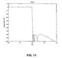
- FIG. 11 is a graph showing a 9 th order filter
- FIG. 12 includes graphs showing the impulse response, h(t), of the 9 th order filter and the individual partial fraction expansion components of the impulse response;
- FIG. 13 is a block diagram of a system implementing the process of FIG. 3 according to the invention.
- FIGS. 1A and 1B show prior art sampling rate conversion process 10 .
- a digital signal x(n) 11 having a first sampling rate T 0 is converted to a digital signal y(n) 12 having a second sampling rate T 1 .
- ⁇ is the impulse function
- k is a sample.
- the signal x c (t) comprises impulses 14 a to 14 c which occur at the same points as the data 11 a in digital signal x(n).
- Filter H(s) 16 converts x c (t) to a continuous-time representation y c (t) 17 of x(n).
- filter 16 is a first order, low-pass filter with a cutoff frequency that is the smaller of n/T 0 and n/T 1 (the Nyquist rate).
- Continuous-to-discrete (C/D) converter 19 then samples y c (t) at rate T 1 to obtain digital signal y(n).
- FIGS. 2A and 2B show how a single data point 20 sampled at T 0 ⁇ x(n) ⁇ is converted to digital signal y(n) 21 sampled at T 1 using the system of FIG. 1 A.
- the continuous-time representation y c (t) 22 for a single data point is a decaying exponential for a first order filter H(s).
- T 0 and T 1 may be time varying relative to the other. That is, T 0 and T 1 may be not be related by a rational number.
- the sampling rate conversion process 25 is shown in FIG. 3 .
- Process 25 obtains ( 301 ) an intermediate sampling value w(n) 26 (FIG. 2C) from input digital signal x(n).
- Value w(n) corresponds to a sample taken at T 1 (the output rate).
- Value w(n) is then digitally filtered ( 302 ) to obtain y(n).
- FIG. 2 D A system diagram 27 for implementing process 25 is shown in FIG. 2 D.
- block 29 includes transfer function H(s) for obtaining w(n) from x(n) and H d (z) 30 , where H d (z) 30 is the filter used to obtain y(n). The following describes how to obtain w(n) from x(n) and then to obtain y(n) from w(n).
- the impulse response, h(t), of a system with function H(s) is
- FIG. 5 The resulting system diagram 31 is shown in FIG. 5, in which H(s) from FIGS. 1A and 2A is replaced by h w (t) 32 and h i (t) 34 .
- C/D converter 35 and h i (t) 34 can be interchanged.
- the resulting system diagram 36 is shown in FIG. 6, in which h i (t) is replaced by its equivalent discrete time filter h d (n) 37 , where
- the output of C/D converter 35 is the intermediate sampling value w(n).
- the value of w(n) may be determined as follows.
- FIG. 7 shows w c (t) 39 and x c (t) 40 for a given x(n) 41 .
- the value for w(n) 42 is sampled from w c (t) at the second/output sampling rate.
- the function w c (t) is a continuous-time representation of the input signal x(n).
- w c (t) is a decaying exponential function that corresponds to x(n).
- FIG. 8 which is a close-up view of w c (t) from FIG. 7 . If the input x(n) is the impulse function ⁇ (n ⁇ n 0 ), then the value of w(n) is h w multiplied by x(n), or
- ⁇ (n ⁇ n 0 T 0 ⁇ ) is the impulse function at time ⁇ n 0 T 0 ⁇ . Defining ⁇ (n) to be “ ⁇ n 0 T 0 ⁇ n 0 T 0 ” (see FIG. 8 for a graphical representation of ⁇ (n)) makes
- w ( n ) h w ( ⁇ ( n 0 )) ⁇ ( n ⁇ n 0 T 0 ⁇ ).
- Evaluating this sum may involve stepping through x(n) one sample at a time, multiplying the resulting value by the coefficient h w ( ⁇ (n)), and then adding the resulting product to the output.
- the coefficient h w ( ⁇ (n)) is obtained by sampling the continuous-time representation h w at ⁇ (n) (see FIG. 8 ), as described below.
- the coefficient h w ( ⁇ (n)) corresponds to the sample x(n), since h w is the continuous-time representation of x(n).
- w(n) is filtered using the digital filter h d (n) 37 (FIG. 6 ). As noted above,
- ⁇ (n) changes as h w (t) changes for each x(n).
- ⁇ (n) (or simply “ ⁇ ”) is defined to be
- ⁇ ( n ) ⁇ ( n ) ⁇ ( n ⁇ 1).
- ⁇ (n) can take on two values: ⁇ (n) either increases by a known quantity, corresponding to a positive value of ⁇ , or ⁇ (n) decreases by a known quantity, corresponding to a negative value of ⁇ . So, ⁇ (n) remains within the range of
- the value of ⁇ in this example is either 0.1 or ⁇ 0.9, depending on the sampling time.
- the difference between a current value of ⁇ nT 0 ⁇ nT 0 ( ⁇ (n)) and a previous value of ⁇ nT 0 ⁇ nT 0 ( ⁇ (n ⁇ 1)) is 0.1 ( ⁇ ).
- the value of ⁇ increases by 0.1 as h w (t) changes over time.
- nT 0 8.1
- ⁇ nT 0 ⁇ 9
- ⁇ nT 0 ⁇ nT 0 0.9
- the new coefficient h w ( ⁇ (n)) can be calculated from the previous coefficient h w ( ⁇ (n ⁇ 1)) in real-time by multiplying h w ( ⁇ (n ⁇ 1)) by the constant ⁇ ⁇ .
- the value of ⁇ ⁇ can be determined beforehand, stored in memory, and then retrieved for the multiplication. Using ⁇ ⁇ to update h w ( ⁇ (n)) eliminates the need to store a table of values for h w ( ⁇ (n)).
- the invention is not limited to use with first order filters.
- a second order filter may be used.
- the system function H(s) 29 in FIG. 2D has one complex conjugate pole pair, one zero on the real axis, and one zero at infinity.
- h ( t ) ⁇ t sin( wt + ⁇ ) u ( t ).
- w c (t) has a time-width of two seconds for the second order case. This is shown in FIG. 10, which shows the second order case 45 in relation to the first order case 46 from FIG. 7 . As shown, in the second order case 45 , w c (t) is a portion (time-limited window) of a sinusoidal function and the two samples 49 and 50 are taken in respective phases 51 and 52 of that sinusoidal function to obtain w(n).
- w ( n ) h w ( ⁇ ( n 0 )) ⁇ ( n ⁇ n 0 T 0 ⁇ )+ h w ( ⁇ ( n 0 )+1) ⁇ ( n ⁇ n 0 T 0 ⁇ 1),
- h w ( ⁇ [ n ]) A ⁇ h w ( ⁇ [ n ⁇ 1])+ B ⁇ h w ( ⁇ [ n ⁇ 1]+1)
- h w ( ⁇ [ n ]+1) C ⁇ h w ( ⁇ [ n ⁇ 1])+ D ⁇ h w ( ⁇ [ n ⁇ 1]+1),
- A ⁇ ⁇ ⁇ ⁇ ( cos ⁇ ⁇ ⁇ + sin ⁇ ⁇ ⁇ cot ⁇ )
- ⁇ is as described above and ⁇ and ⁇ are known second order filter properties.
- the constants A, B, C and D can be determined beforehand, stored in memory, and retrieved when it comes time to perform the necessary multiplication. For each sample, new coefficients h w ( ⁇ (n)) and h w ( ⁇ (n)+1) are determined in real-time from the old coefficients h w ( ⁇ (n ⁇ 1)) and h w ( ⁇ (n ⁇ 1)+1) using only four multiplication operations, i.e., by A, B, C and D. Since there are two possible values for ⁇ (as above), two different version of A, B, C and D should be determined, stored, and applied as appropriate.
- the invention can be used with higher order filters as well.
- H(s) has N (N>2) poles and N ⁇ 1 zeros in the finite s-plane.
- a partial fraction expansion can be performed on H(s) to break down H(s) into the sum of several first and/or second order pieces, each of which can be solved as described above. Each of these pieces can be implemented in parallel and the results added together to find a solution to the Nth order case.
- N r is the number of real poles and N p is the number of complex conjugate pole pairs.
- H(s) has repeated poles.
- each of the intermediate sampling values w(n) are obtained ( 301 ) by obtaining ( 301 a ) the coefficients, h w , that are needed from the continuous-time representation of the input signal.
- N (N ⁇ 1) total poles N such coefficients will be needed.
- Values for w(n) are determined ( 301 b ) by stepping through the input samples one at a time and, at each step (i) multiplying the value of the sample by the coefficients h w and adding the results to w(n), and (ii) updating the coefficients h w in preparation for the next iteration.
- w(n) is filtered ( 302 ) using an appropriate filter and the results of the filtering summed to obtain output y(n).
- H(s) is chosen to be an elliptic filter with a passband edge frequency of 2 ⁇ (20 kHz/44.1 kHz) radians per second and a stopband edge frequency of 2 ⁇ (24.1 kHz/44.1 kHz) radians per second.
- the passband is allowed ⁇ 0.2 dB (decibels) of ripple and the stopband is allowed at least 80 dB of attenuation.
- a 9 th order elliptic filter having the response shown in FIG. 11 is used.
- the impulse response h(t) and its individual partial fraction components h 1 (t) to h 5 (t) are shown in FIG. 12 .
- process 25 For generating the values of w(n), process 25 performs one multiplication operation per sample for the real pole. Process 25 performs two multiplication operations for each of the four-pole pairs. These are performed twice because there are two channels. Thus, a total of eighteen multiplication operations are performed for every sample to generate values of w(n). To update the h w coefficients, one multiplication operation is performed for the real pole and four multiplication operations are performed for each of the pole pairs, for a total of seventeen multiplication operations. To filter the values of w(n) to obtain the output y(n), nine multiplication operations are performed for each of the two channels, adding a total of eighteen more multiplication operations. Thus, process 25 performs a total of 53 multiplication operations. In real time, these multiplication operations are performed for every sample, i.e., 44,100 times per second, for a total of 2.34 million multiplication operations per second.
- FIG. 13 shows a device 55 (e.g., a computer) for performing sampling rate conversion process 25 .
- Device 55 includes a processor 56 , a memory 57 , and a,storage medium 59 , e.g., a hard disk (see view 60 ).
- Storage medium 59 stores computer-executable instructions 61 for performing process 25 .
- Processor 56 executes computer-executable instructions 61 out of memory 57 to perform process 25 .
- Process 25 is not limited to use with the hardware/software configuration of FIG. 13; it may find applicability in any computing or processing environment.
- Process 25 may be implemented in hardware, software, or a combination of the two (e.g., using an ASIC (application-specific integrated circuit) or programmable logic).
- Process 25 may be implemented in one or more computer programs executing on programmable computers that each includes a processor, a storage medium readable by the processor (including volatile and non-volatile memory and/or storage elements), at least one input device, and one or more output devices.
- Program code may be applied to data entered using an input device to perform process 25 and to generate output information.
- the output information may be applied to one or more output devices.
- Each such program may be implemented in a high level procedural or object-oriented programming language to communicate with a computer system.
- the programs can be implemented in assembly or machine language.
- the language may be a compiled or an interpreted language.
- Each computer program may be stored on a storage medium or device (e.g., CD-ROM, hard disk, or magnetic diskette) that is readable by a general or special purpose programmable computer for configuring and operating the computer when the storage medium or device is read by the computer to perform process 25 .
- Process 25 may also be implemented as a computer-readable storage medium, configured with a computer program, where, upon execution, instructions in the computer program cause the computer to operate in accordance with process 25 .
- an input signal whose sampling rate is to be converted may be partitioned into blocks. After each block, new h w coefficients are determined. This block-based approach permits changing of the sampling rate T 0 for each block.
- the invention can be used to mix digital signals from any asynchronous sources in real-time, not just digital audio.
Landscapes
- Physics & Mathematics (AREA)
- Engineering & Computer Science (AREA)
- Computer Hardware Design (AREA)
- Mathematical Physics (AREA)
- Analogue/Digital Conversion (AREA)
Abstract
An input signal having a first sampling rate is converted to an output signal having a second sampling rate. This is done by obtaining an intermediate sampling value from the input signal and filtering the intermediate sampling value to obtain the output signal. The intermediate sampling value corresponds to a sample taken at the second sampling rate on a continuous-time representation of the input signal.
Description
Not Applicable
Not Applicable
Not Applicable
This invention relates to converting an input data stream having a first sampling rate to an output data stream having a second sampling rate.
Sampling rate conversion is performed when a discrete-time system needs to combine data streams with differing sampling rates. This is a common occurrence in audio and video applications. For example, audio sources may occur at different sampling rates, such as 44.1 kHz (kilohertz) for compact disks (CDs) and 48 kHz for digital audio tape (DAT).
One way of performing sampling rate conversion is to use a combination of up-sampling, filtering, and down-sampling. This can work if the ratio of the two sampling rates equals a rational number. In many cases, however, the two sampling rates are not related by a simple rational number. This occurs frequently when trying to synchronize data streams that are arriving from separate digital networks. For example, in audio applications, it is common to have a discrete-time system operating at 44.1 kHz while its input data stream is arriving at roughly 44.09 kHz with time variations. The receiving portion of the discrete-time system must adjust for these time variations during sampling rate conversion.
One way of performing sampling rate conversions on time-varying data streams uses finite impulse response (FIR) filters and linear weighted interpolation based on neighboring samples.
It is an important object to provide improved sampling rate conversion.
In general, in one aspect, the invention is directed to converting an input signal having a first sampling rate to an output signal having a second sampling rate. The invention features obtaining an intermediate sampling value from the input signal and filtering the intermediate sampling value to obtain the output signal. The intermediate sampling value corresponds to a sample taken at the second sampling rate on a continuous-time representation of the input signal.
This aspect of the invention may include one or more of the following features. Obtaining the intermediate sampling value includes obtaining a coefficient that corresponds to the sample from the continuous-time representation of the input signal and determining the intermediate sampling value based on the coefficient and an impulse value. The impulse value corresponds to the input signal. The coefficient is a value of the continuous-time representation of the input signal taken at the sample. The coefficient is determined from a previous coefficient by multiplying the previous coefficient by a constant. The constant corresponds to a difference between the sample and a previous sample.
Filtering the intermediate sampling value includes adding the intermediate sampling value to a previous value that corresponds to a previous sample taken at the second sampling rate. Filtering is performed by a first order digital filter.
A second intermediate sampling value is obtained from the input signal and the second intermediate sampling value is filtered to obtain the output signal. The second intermediate sampling value corresponds to a second sample taken at the second sampling rate on the continuous-time representation of the input signal. In this case, filtering is performed using a second order digital filter.
One of the first and second sampling rates may be a compact disk sampling rate and the other of the first and second sampling rates may be a digital audio tape sampling rate. The continuous-time representation of the input signal may be a decaying exponential function or a sinusoidal function.
Other features, objects and advantages of the invention will become apparent from the following description and drawings.
FIG. 1A is a system diagram of a prior art sampling rate conversion process; and FIG. 1B shows graphs of the signals included in the system diagram of FIG. 1A;
FIG. 2A is a system diagram of the prior art sampling rate conversion process; FIG. 2B shows graphs of the signals included in the system diagram of FIG. 2A; FIG. 2C shows an intermediate sampling value obtained from an input signal according to the invention; and FIG. 2D is a system diagram of a sampling rate conversion process that uses the intermediate sampling value according to the invention;
FIG. 3 is a flowchart showing the sampling rate conversion process that uses the intermediate sampling value according to the invention;
FIG. 4 shows the impulse response h(t) broken down into separate components hw(t) and hi(t);
FIG. 5 is a system diagram of a sampling rate conversion process that includes the separate components hw(t) and hi(t);
FIG. 6 a system diagram of a sampling rate conversion process that is derived from the system diagram of FIG. 5 and that includes the intermediate sampling value according to the invention;
FIG. 7 shows signals present in the system of FIG. 6 when a first order digital filter is used;
FIG. 8 is a close-up view of signal wc(t) from FIG. 7;
FIGS. 9A through 9F are graphs showing how wc(t) varies over time;
FIG. 10 shows signals present in the system of FIG. 6 when a second order digital filter is used;
FIG. 11 is a graph showing a 9th order filter;
FIG. 12 includes graphs showing the impulse response, h(t), of the 9th order filter and the individual partial fraction expansion components of the impulse response; and
FIG. 13 is a block diagram of a system implementing the process of FIG. 3 according to the invention.
With reference now to the drawings, FIGS. 1A and 1B show prior art sampling rate conversion process 10. In those figures, a digital signal x(n) 11 having a first sampling rate T0 is converted to a digital signal y(n) 12 having a second sampling rate T1. The conversion process 10 includes generating a time-based signal xc(t) 14 using discrete-to-continuous (D/C) converter 15, where xc(t) is: 
δ is the impulse function, and k is a sample.
The signal xc(t) comprises impulses 14 a to 14 c which occur at the same points as the data 11 a in digital signal x(n). Filter H(s) 16 converts xc(t) to a continuous-time representation yc(t) 17 of x(n). In this example, filter 16 is a first order, low-pass filter with a cutoff frequency that is the smaller of n/T0 and n/T1 (the Nyquist rate). Continuous-to-discrete (C/D) converter 19 then samples yc(t) at rate T1 to obtain digital signal y(n).
FIGS. 2A and 2B show how a single data point 20 sampled at T0 {x(n)} is converted to digital signal y(n) 21 sampled at T1 using the system of FIG. 1A. The continuous-time representation yc(t) 22 for a single data point is a decaying exponential for a first order filter H(s). One or both of T0 and T1 may be time varying relative to the other. That is, T0 and T1 may be not be related by a rational number.
The sampling rate conversion process 25 according to the invention is shown in FIG. 3. Process 25 obtains (301) an intermediate sampling value w(n) 26 (FIG. 2C) from input digital signal x(n). Value w(n) corresponds to a sample taken at T1 (the output rate). Value w(n) is then digitally filtered (302) to obtain y(n).
A system diagram 27 for implementing process 25 is shown in FIG. 2D. In system diagram 27, block 29 includes transfer function H(s) for obtaining w(n) from x(n) and Hd(z) 30, where Hd(z) 30 is the filter used to obtain y(n). The following describes how to obtain w(n) from x(n) and then to obtain y(n) from w(n).
Assume that H(s) in block 29 is a first order filter with a system function of 
H(s) thus has a pole at s=−a and a zero at infinity. The impulse response, h(t), of a system with function H(s) is
where u(t) is the unit step function defined by 
If “a” is real and positive then, by definition, the impulse response h(t) is real and the system is stable. Also assume that T1=1. This does not restrict sampling rate conversion process 25, since any change in the sampling rate can be achieved by choosing an appropriate value for T0.
The impulse response h(t) of system 27 (FIG. 4A) can be represented as a finite-duration or time-limited window hw(t) (FIG. 4B) convolved with a train of decaying impulses hi(t) (FIG. 4C). More specifically, 
where α=e−a, 
The resulting system diagram 31 is shown in FIG. 5, in which H(s) from FIGS. 1A and 2A is replaced by hw(t) 32 and hi(t) 34.
If the sampling performed by C/D converter 35 and the impulses in hi(t) are both spaced by one second in time, C/D converter 35 and hi(t) 34 can be interchanged. The resulting system diagram 36 is shown in FIG. 6, in which hi(t) is replaced by its equivalent discrete time filter hd(n) 37, where
The output of C/D converter 35 is the intermediate sampling value w(n). The value of w(n) may be determined as follows.
Assuming that x(n)=δ(n−n0) and xc(t)=δ(t−n0T0), then wc(t)=hw(t−n0T0), which starts at time n0T0 and has a duration of one second. FIG. 7 shows wc(t) 39 and xc(t) 40 for a given x(n) 41. The value for w(n) 42 is sampled from wc(t) at the second/output sampling rate. The function wc(t) is a continuous-time representation of the input signal x(n). For a first order filter, as in this example, wc(t) is a decaying exponential function that corresponds to x(n).
C/D converter 35 (FIG. 6) has a single nonzero output at a time n=┌n0T0┐, where the notation “┌n0T0┐” indicates the smallest integer value that is greater than or equal to n0T0. This is so because C/D converter 35 samples at integer time values only. The amplitude of the sample of w(n) will thus be
as shown in FIG. 8 (which is a close-up view of wc(t) from FIG. 7). If the input x(n) is the impulse function δ(n−n0), then the value of w(n) is hw multiplied by x(n), or
where δ(n−┌n0T0┐) is the impulse function at time ┌n0T0┐. Defining τ(n) to be “┌n0T0┐−n0T0” (see FIG. 8 for a graphical representation of τ(n)) makes
To determine the response of the system to an input x(n), where x(n) contains multiple nonzero samples m, the equation is as follows 
Evaluating this sum may involve stepping through x(n) one sample at a time, multiplying the resulting value by the coefficient hw(τ(n)), and then adding the resulting product to the output. The coefficient hw(τ(n)) is obtained by sampling the continuous-time representation hw at τ(n) (see FIG. 8), as described below. The coefficient hw(τ(n)) corresponds to the sample x(n), since hw is the continuous-time representation of x(n).
To obtain y(n) from w(n), w(n) is filtered using the digital filter hd(n) 37 (FIG. 6). As noted above,
h d(n)=αn u(n).
Taking the Z-transform of hd(n) yields
Rearranging the terms and taking the inverse Z transform of Hd(z) leads to the difference equation
which defines the filter for obtaining y(n) from w(n).
The following describes determining the values of hw(τ(n)) that are used in determining w(n).
The value of τ(n) changes as hw(t) changes for each x(n). To determine how τ(n) changes over time, Δ(n) (or simply “Δ”) is defined to be
Noting that τ(n)=┌n0T0┐−n0T0, results in the following 
Thus, Δ(n) can take on two values: τ(n) either increases by a known quantity, corresponding to a positive value of Δ, or τ(n) decreases by a known quantity, corresponding to a negative value of Δ. So, τ(n) remains within the range of
FIGS. 9A to 9F show shifted and scaled copies of hw(t). For sample n=1, nT0=0.9 (FIG. 9B); for sample n=2, nT0=1.8 (FIG. 9C); for sample n=3, nT0=2.7 (FIG. 9D); and so on. The value of Δ in this example is either 0.1 or −0.9, depending on the sampling time. That is, for nT0=0.9, ┌nT0┐ is 1 and ┌nT0┐−nT0 (i.e., τ(n)) is 0.1; for nT0=1.8, ┌nT0┐ is 2 and ┌nT0┐−nT0 is 0.2; for nT0=2.7, ┌nT0┐ is 3 and ┌nT0┐−nT0 is 0.3; and so on. The difference between a current value of ┌nT0┐−nT0 (τ(n)) and a previous value of ┌nT0┐−nT0 (τ(n−1))is 0.1 (Δ). Thus, in this example, the value of Δ increases by 0.1 as hw(t) changes over time. Alternatively, when nT0=8.1, ┌nT0┐ is 9, and ┌nT0┐−nT0 is 0.9. Following this progression leads to a Δ value of −0.9.
Knowing the value of Δ, it is possible to determine τ(n) from τ(n−1) and, thus, to determine hw(τ(n)) from hw(τ(n−1)) and Δ. More specifically, from above, 
Thus, at each sample, the new coefficient hw(τ(n)) can be calculated from the previous coefficient hw(τ(n−1)) in real-time by multiplying hw(τ(n−1)) by the constant αΔ. The value of αΔ can be determined beforehand, stored in memory, and then retrieved for the multiplication. Using αΔ to update hw(τ(n)) eliminates the need to store a table of values for hw(τ(n)).
The foregoing describes sampling rate conversion using a first order digital filter hd(n). The invention, however, is not limited to use with first order filters. For example, a second order filter may be used. In the case of a second order filter, assume that the system function H(s) 29 in FIG. 2D has one complex conjugate pole pair, one zero on the real axis, and one zero at infinity. For such a system,
Representing the impulse response of the second order system as the convolution of a time limited portion hw(t) and an infinite train of impulses yields 
where
and 
As above, interchanging the filtering and sampling operations yields the system shown in FIG. 6, where 
When x(n)=δ(n−n0), wc(t) has a time-width of two seconds for the second order case. This is shown in FIG. 10, which shows the second order case 45 in relation to the first order case 46 from FIG. 7. As shown, in the second order case 45, wc(t) is a portion (time-limited window) of a sinusoidal function and the two samples 49 and 50 are taken in respective phases 51 and 52 of that sinusoidal function to obtain w(n).
The first of the samples 49 occurs at t=┌n0T0┐ and the second of these samples 50 occurs at t=┌n0T0┐+1. The amplitude of first sample 49 is hw(τ(n0)) and the amplitude of second sample 50 is hw(τ(n0)+1). So, for an input of x(n)=δ(n−n0),
This is analogous to the equation for w(n) described for first order filters above. For an arbitrary input x(m), the intermediate sampling value w(n) is as follows 
The equations for determining the first coefficient hw(τ(n)) and the second coefficient hw(τ(n)+1) are as follows:
where 
In the foregoing equations, Δ is as described above and γ and ω are known second order filter properties.
As above, the constants A, B, C and D can be determined beforehand, stored in memory, and retrieved when it comes time to perform the necessary multiplication. For each sample, new coefficients hw(τ(n)) and hw(τ(n)+1) are determined in real-time from the old coefficients hw(τ(n−1)) and hw(τ(n−1)+1) using only four multiplication operations, i.e., by A, B, C and D. Since there are two possible values for Δ (as above), two different version of A, B, C and D should be determined, stored, and applied as appropriate.
To obtain the digital filter hd(n) for the second order case, we take the Z transform of 
to obtain 
Rearranging the terms and taking the inverse Z transform of Hd(Z) leads to the difference equation
This involves only two multiplication operations per sample to obtain y(n) from w(n).
The invention can be used with higher order filters as well. For example, assume that H(s) has N (N>2) poles and N−1 zeros in the finite s-plane. A partial fraction expansion can be performed on H(s) to break down H(s) into the sum of several first and/or second order pieces, each of which can be solved as described above. Each of these pieces can be implemented in parallel and the results added together to find a solution to the Nth order case. To implement the Nth order case, the impulse response of the system is defined as 
where Nr is the number of real poles and Np is the number of complex conjugate pole pairs. A similar process may be used for the case where H(s) has repeated poles.
To summarize, the sampling rate conversion process for a given H(s) having Nr real poles and Np pairs of complex conjugate poles (for a total N poles) is as set forth in FIG. 3. That is, each of the intermediate sampling values w(n) are obtained (301) by obtaining (301 a) the coefficients, hw, that are needed from the continuous-time representation of the input signal. For N (N≧1) total poles, N such coefficients will be needed. Values for w(n) are determined (301 b) by stepping through the input samples one at a time and, at each step (i) multiplying the value of the sample by the coefficients hw and adding the results to w(n), and (ii) updating the coefficients hw in preparation for the next iteration. After values for w(n) have been obtained, w(n) is filtered (302) using an appropriate filter and the results of the filtering summed to obtain output y(n).
The following describes process 25 as performed on two digital audio streams that are to be combined and output through the same DAC (digital-to-analog converter). Each input is a two-channel audio stream. However, one of the inputs is arriving at 44.1 kHz and the other is arriving at 44.09794 kHz. Process 25 is used to up-sample the second input by a fraction T0=0.9995328.
To do this, H(s) is chosen to be an elliptic filter with a passband edge frequency of 2π(20 kHz/44.1 kHz) radians per second and a stopband edge frequency of 2π(24.1 kHz/44.1 kHz) radians per second. The passband is allowed ±0.2 dB (decibels) of ripple and the stopband is allowed at least 80 dB of attenuation. To match these specifications, a 9th order elliptic filter having the response shown in FIG. 11 is used. The impulse response h(t) and its individual partial fraction components h1(t) to h5(t) are shown in FIG. 12.
For generating the values of w(n), process 25 performs one multiplication operation per sample for the real pole. Process 25 performs two multiplication operations for each of the four-pole pairs. These are performed twice because there are two channels. Thus, a total of eighteen multiplication operations are performed for every sample to generate values of w(n). To update the hw coefficients, one multiplication operation is performed for the real pole and four multiplication operations are performed for each of the pole pairs, for a total of seventeen multiplication operations. To filter the values of w(n) to obtain the output y(n), nine multiplication operations are performed for each of the two channels, adding a total of eighteen more multiplication operations. Thus, process 25 performs a total of 53 multiplication operations. In real time, these multiplication operations are performed for every sample, i.e., 44,100 times per second, for a total of 2.34 million multiplication operations per second.
In a standard FIR sampling conversion technique, a time-varying impulse response having a length of twenty-seven is required (thirty-one if it is a linear phase). So,twenty-seven multiplication operations per channel are needed. This leads to about 2.38 million multiplication operations per second, which is comparable to the number of multiplication operations required by process 25. The difference, however, is that the FIR technique requires a large table of impulse responses/coefficients to be stored. Such a table is on the order of seven thousand points. For process 25, only about fifty-two values (e.g., Δ, A, B, C and D above) are stored. Thus, relatively little memory is needed to perform the sampling rate conversion process of the invention.
FIG. 13 shows a device 55 (e.g., a computer) for performing sampling rate conversion process 25. Device 55 includes a processor 56, a memory 57, and a,storage medium 59, e.g., a hard disk (see view 60). Storage medium 59 stores computer-executable instructions 61 for performing process 25. Processor 56 executes computer-executable instructions 61 out of memory 57 to perform process 25.
Process 25, however, is not limited to use with the hardware/software configuration of FIG. 13; it may find applicability in any computing or processing environment. Process 25 may be implemented in hardware, software, or a combination of the two (e.g., using an ASIC (application-specific integrated circuit) or programmable logic). Process 25 may be implemented in one or more computer programs executing on programmable computers that each includes a processor, a storage medium readable by the processor (including volatile and non-volatile memory and/or storage elements), at least one input device, and one or more output devices. Program code may be applied to data entered using an input device to perform process 25 and to generate output information. The output information may be applied to one or more output devices.
Each such program may be implemented in a high level procedural or object-oriented programming language to communicate with a computer system. However, the programs can be implemented in assembly or machine language. The language may be a compiled or an interpreted language.
Each computer program may be stored on a storage medium or device (e.g., CD-ROM, hard disk, or magnetic diskette) that is readable by a general or special purpose programmable computer for configuring and operating the computer when the storage medium or device is read by the computer to perform process 25. Process 25 may also be implemented as a computer-readable storage medium, configured with a computer program, where, upon execution, instructions in the computer program cause the computer to operate in accordance with process 25.
Other embodiments not described herein are also within the scope of the following claims. For example, an input signal whose sampling rate is to be converted may be partitioned into blocks. After each block, new hw coefficients are determined. This block-based approach permits changing of the sampling rate T0 for each block. The invention can be used to mix digital signals from any asynchronous sources in real-time, not just digital audio.
Representative Matlab code for performing sampling rate conversion in accordance with process 25 using an Nth (N>1) order filter is shown in the attached Appendix.
Claims (43)
1. A method of converting an input signal having a first sampling rate to an output signal having a second sampling rate, comprising:
obtaining an intermediate sampling value from the input signal, the intermediate sampling value corresponding to a sample taken at the second sampling rate on a continuous-time representation of the input signal; and
filtering the intermediate sampling value to obtain the output signal.
2. The method of claim 1 , wherein obtaining the intermediate sampling value comprises:
obtaining a coefficient from the continuous-time representation of the input signal, the coefficient corresponding to the sample; and
determining the intermediate sampling value based on the coefficient and an impulse value.
3. The method of claim 2 , wherein the impulse value corresponds to the input signal.
4. The method of claim 2 , wherein the coefficient comprises a value of the continuous-time representation of the input signal taken at the sample.
5. The method of claim 4 , wherein the coefficient is determined from a previous coefficient by multiplying the previous coefficient by a constant.
6. The method of claim 5 , wherein the constant corresponds to a difference between the sample and a previous sample.
7. The method of claim 1 , wherein filtering comprises adding the intermediate sampling value to a previous value that corresponds to a previous sample taken at the second sampling rate.
8. The method of claim 1 , wherein filtering is performed by a first order digital filter.
9. The method of claim 1 , further comprising:
obtaining a second intermediate sampling value from the input signal, the second intermediate sampling value corresponding to a second sample taken at the second sampling rate on the continuous-time representation of the input signal; and
filtering the second intermediate sampling value to obtain the output signal.
10. The method of claim 9 , wherein filtering is performed using a second order digital filter.
11. The method of claim 1 , wherein one of the first and second sampling rates comprises a compact disk sampling rate and the other of the first and second sampling rates comprises a digital audio tape sampling rate.
12. The method of claim 1 , wherein the continuous-time representation of the input signal comprises a decaying exponential function.
13. The method of claim 1 , wherein the continuous-time representation of the input signal comprises a sinusoidal function.
14. The method of claim 1 , wherein one of the first and second sampling rates is time-varying.
15. A computer program stored on a computer-readable medium for converting an input signal having a first sampling rate to an output signal having a second sampling rate, the computer program comprising executable instructions that cause a computer to:
obtain an intermediate sampling value from the input signal, the intermediate sampling value corresponding to a sample taken at the second sampling rate on a continuous-time representation of the input signal; and
filter the intermediate sampling value to obtain the output signal.
16. The computer program of claim 15 , wherein obtaining the intermediate sampling value comprises:
obtaining a coefficient from the continuous-time representation of the input signal, the coefficient corresponding to the sample; and
determining the intermediate sampling value based on the coefficient and an impulse value.
17. The computer program of claim 16 , wherein the impulse value corresponds to the input signal.
18. The computer program of claim 16 , wherein the coefficient comprises a value of the continuous-time representation of the input signal taken at the sample.
19. The computer program of claim 18 , wherein the coefficient is determined from a previous coefficient by multiplying the previous coefficient by a constant.
20. The computer program of claim 19 , wherein the constant corresponds to a difference between the sample and a previous sample.
21. The computer program of claim 15 , wherein filtering comprises adding the intermediate sampling value to a previous value that corresponds to a previous sample taken at the second sampling rate.
22. The computer program of claim 15 , wherein filtering is performed by a first order digital filter.
23. The computer program of claim 15 , further comprising instructions that cause the computer to:
obtain a second intermediate sampling value from the input signal, the second intermediate sampling value corresponding to a second sample taken at the second sampling rate on the continuous-time representation of the input signal; and
filter the second intermediate sampling value to obtain the output signal.
24. The computer program of claim 23 , wherein filtering is performed using a second order digital filter.
25. The computer program of claim 15 , wherein one of the first and second sampling rates comprises a compact disk sampling rate and the other of the first and second sampling rates comprises a digital audio tape sampling rate.
26. The computer program of claim 15 , wherein the continuous-time representation of the input signal comprises a decaying exponential function.
27. The computer program of claim 15 , wherein the continuous-time representation of the input signal comprises a sinusoidal function.
28. The computer program of claim 15 , wherein one of the first and second sampling rates is time-varying.
29. An apparatus for converting an input signal having a first sampling rate to an output signal having a second sampling rate, that apparatus comprising circuitry which:
obtains an intermediate sampling value from the input signal, the intermediate sampling value corresponding to a sample taken at the second sampling rate on a continuous-time representation of the input signal; and
filters the intermediate sampling value to obtain the output signal.
30. The apparatus of claim 29 , wherein obtaining the intermediate sampling value comprises:
obtaining a coefficient from the continuous-time representation of the input signal, the coefficient corresponding to the sample; and
determining the intermediate sampling value based on the coefficient and an impulse value.
31. The apparatus of claim 30 , wherein the impulse value corresponds to the input signal.
32. The apparatus of claim 29 , wherein the coefficient comprises a value of the continuous-time representation of the input signal taken at the sample.
33. The apparatus of claim 32 , wherein the coefficient is determined from a previous coefficient by multiplying the previous coefficient by a constant.
34. The apparatus of claim 33 , wherein the constant corresponds to a difference between the sample and a previous sample.
35. The apparatus of claim 29 , wherein filtering comprises adding the intermediate sampling value to a previous value that corresponds to a previous sample taken at the second sampling rate.
36. The apparatus of claim 29 , wherein filtering is performed by a first order digital filter.
37. The apparatus of claim 29 , further comprising circuitry which:
obtains a second intermediate sampling value from the input signal, the second intermediate sampling value corresponding to a second sample taken at the second sampling rate on the continuous-time representation of the input signal; and
filters the second intermediate sampling value to obtain the output signal.
38. The apparatus of claim 37 , wherein filtering is performed using a second order digital filter.
39. The apparatus of claim 29 , wherein one of the first and second sampling rates comprises a compact disk sampling rate and the other of the first and second sampling rates comprises a digital audio tape sampling rate.
40. The apparatus of claim 29 , wherein the continuous-time representation of the input signal comprises a decaying exponential function.
41. The apparatus of claim 29 , wherein the continuous-time representation of the input signal comprises a sinusoidal function.
42. The apparatus of claim 29 , wherein one of the first and second sampling rates is time-varying.
43. An apparatus for converting an input signal having a first sampling rate to an output signal having a second sampling rate, comprising:
means for obtaining an intermediate sampling value from the input signal, the intermediate sampling value corresponding to a sample taken at the second sampling rate on a continuous-time representation of the input signal; and
means for filtering the intermediate sampling value to obtain the output signal.
Priority Applications (1)
| Application Number | Priority Date | Filing Date | Title |
|---|---|---|---|
| US09/684,041 US6665694B1 (en) | 2000-10-06 | 2000-10-06 | Sampling rate conversion |
Applications Claiming Priority (1)
| Application Number | Priority Date | Filing Date | Title |
|---|---|---|---|
| US09/684,041 US6665694B1 (en) | 2000-10-06 | 2000-10-06 | Sampling rate conversion |
Publications (1)
| Publication Number | Publication Date |
|---|---|
| US6665694B1 true US6665694B1 (en) | 2003-12-16 |
Family
ID=29712556
Family Applications (1)
| Application Number | Title | Priority Date | Filing Date |
|---|---|---|---|
| US09/684,041 Expired - Lifetime US6665694B1 (en) | 2000-10-06 | 2000-10-06 | Sampling rate conversion |
Country Status (1)
| Country | Link |
|---|---|
| US (1) | US6665694B1 (en) |
Cited By (4)
| Publication number | Priority date | Publication date | Assignee | Title |
|---|---|---|---|---|
| US20040114750A1 (en) * | 2002-12-16 | 2004-06-17 | Leblanc Wilf | Switchboard for dual-rate single-band communication system |
| US6889365B2 (en) * | 1998-08-10 | 2005-05-03 | Fujitsu Limited | Terminal operation apparatus |
| WO2007084687A1 (en) * | 2006-01-18 | 2007-07-26 | Dolby Laboratories Licensing Corporation | Asynchronous sample rate conversion using a digital simulation of an analog filter |
| EP3716479A1 (en) | 2019-03-26 | 2020-09-30 | Bang & Olufsen A/S | A method for sampling rate conversion |
Citations (3)
| Publication number | Priority date | Publication date | Assignee | Title |
|---|---|---|---|---|
| US6134569A (en) * | 1997-01-30 | 2000-10-17 | Sharp Laboratories Of America, Inc. | Polyphase interpolator/decimator using continuous-valued, discrete-time signal processing |
| US6182101B1 (en) * | 1993-12-08 | 2001-01-30 | Nokia Mobile Phones, Ltd. | Method for sampling frequency conversion employing weighted averages |
| US20020046227A1 (en) * | 2000-06-02 | 2002-04-18 | Goszewski Cynthia P. | Sampling rate converter and method |
-
2000
- 2000-10-06 US US09/684,041 patent/US6665694B1/en not_active Expired - Lifetime
Patent Citations (3)
| Publication number | Priority date | Publication date | Assignee | Title |
|---|---|---|---|---|
| US6182101B1 (en) * | 1993-12-08 | 2001-01-30 | Nokia Mobile Phones, Ltd. | Method for sampling frequency conversion employing weighted averages |
| US6134569A (en) * | 1997-01-30 | 2000-10-17 | Sharp Laboratories Of America, Inc. | Polyphase interpolator/decimator using continuous-valued, discrete-time signal processing |
| US20020046227A1 (en) * | 2000-06-02 | 2002-04-18 | Goszewski Cynthia P. | Sampling rate converter and method |
Non-Patent Citations (1)
| Title |
|---|
| Ramstad, Digital Methods for Conversion Between Arbitrary Sampling Frequencies IEE Transactions on Acoustics, Speech, and Signal Processing, Vo. ASSP-32, No. 3 Jun. 1984, 577-91. |
Cited By (11)
| Publication number | Priority date | Publication date | Assignee | Title |
|---|---|---|---|---|
| US6889365B2 (en) * | 1998-08-10 | 2005-05-03 | Fujitsu Limited | Terminal operation apparatus |
| US20080291940A1 (en) * | 2002-09-27 | 2008-11-27 | Leblanc Wilf | Switchboard For Dual-Rate Single-Band Communication System |
| US8155285B2 (en) | 2002-09-27 | 2012-04-10 | Broadcom Corporation | Switchboard for dual-rate single-band communication system |
| US20040114750A1 (en) * | 2002-12-16 | 2004-06-17 | Leblanc Wilf | Switchboard for dual-rate single-band communication system |
| US7409056B2 (en) * | 2002-12-16 | 2008-08-05 | Broadcom Corporation | Switchboard for dual-rate single-band communication system |
| WO2007084687A1 (en) * | 2006-01-18 | 2007-07-26 | Dolby Laboratories Licensing Corporation | Asynchronous sample rate conversion using a digital simulation of an analog filter |
| US20090079599A1 (en) * | 2006-01-18 | 2009-03-26 | Dolby Laboratories Licensing Corporation | Asynchronous Sample Rate Conversion Using a Digital Simulation of an Analog Filter |
| US7619546B2 (en) * | 2006-01-18 | 2009-11-17 | Dolby Laboratories Licensing Corporation | Asynchronous sample rate conversion using a digital simulation of an analog filter |
| EP3716479A1 (en) | 2019-03-26 | 2020-09-30 | Bang & Olufsen A/S | A method for sampling rate conversion |
| EP3716480A1 (en) | 2019-03-26 | 2020-09-30 | Bang & Olufsen A/S | A method and an apparatus for sampling rate conversion |
| US11581874B2 (en) | 2019-03-26 | 2023-02-14 | Bang & Olufsen A/S | Method and an apparatus for sampling rate conversion |
Similar Documents
| Publication | Publication Date | Title |
|---|---|---|
| EP2417701B1 (en) | Obtaining a desired non-zero phase shift using forward-backward filtering | |
| JPH0642619B2 (en) | Interpolative time-discrete filter device | |
| US20070094317A1 (en) | Method and system for B-spline interpolation of a one-dimensional signal using a fractional interpolation ratio | |
| CN108763720B (en) | DDC implementation method with sampling rate capable of being adjusted down at will | |
| US7010557B2 (en) | Low power decimation system and method of deriving same | |
| US8489661B2 (en) | Signal processing system with a digital sample rate converter | |
| US6665694B1 (en) | Sampling rate conversion | |
| EP1295390B1 (en) | Universal sampling rate converter for digital audio frequencies | |
| US6766338B1 (en) | High order lagrange sample rate conversion using tables for improved efficiency | |
| Russell et al. | Efficient arbitrary sampling rate conversion with recursive calculation of coefficients | |
| JPH06350399A (en) | Method and digital filter architecture for filtering digital signal | |
| Hogenauer | A class of digital filters for decimation and interpolation | |
| US6058404A (en) | Apparatus and method for a class of IIR/FIR filters | |
| WO2003047097A1 (en) | Digital filter designing method, designing apparatus, digital filter designing program, digital filter | |
| US7292630B2 (en) | Limit-cycle-free FIR/IIR halfband digital filter with shared registers for high-speed sigma-delta A/D and D/A converters | |
| JPH0590897A (en) | Oversampling filter circuit | |
| JPH0732344B2 (en) | Thinning filter | |
| WO2004036746A1 (en) | Digital filter design method and device, digital filter design program, and digital filter | |
| US7002997B2 (en) | Interpolation filter structure | |
| CN1191537C (en) | Device and method for anchoring physics to realize predetermined point of filter impulse frequency response | |
| EP1033812B1 (en) | Oversampling structure with frequency response of the sinc type | |
| JPH0472905A (en) | Sampling frequency converter | |
| US8823559B2 (en) | Shift-invariant digital sampling rate conversion system | |
| JPH10308650A (en) | Filter design method and digital filter | |
| JP3258938B2 (en) | Decimation filter |
Legal Events
| Date | Code | Title | Description |
|---|---|---|---|
| AS | Assignment |
Owner name: BOSE CORPORATION, MASSACHUSETTS Free format text: ASSIGNMENT OF ASSIGNORS INTEREST;ASSIGNORS:RUSSELL, ANDREW;BECKMANN, PAUL ERIC;REEL/FRAME:011261/0160 Effective date: 20001002 |
|
| STCF | Information on status: patent grant |
Free format text: PATENTED CASE |
|
| FPAY | Fee payment |
Year of fee payment: 4 |
|
| FPAY | Fee payment |
Year of fee payment: 8 |
|
| FPAY | Fee payment |
Year of fee payment: 12 |