Abstract
We consider a multivariate Markov-switching GARCH model which allows for regime-specific volatility dynamics, leverage effects, and correlation structures. Conditions for stationarity and expressions for the moments of the process are derived. A Lagrange Multiplier test against misspecification of the within-regime correlation dynamics is proposed, and a simple recursion for multi-step-ahead conditional covariance matrices is deduced. We use this methodology to model the dynamics of the joint distribution of global stock market and real estate equity returns. The empirical analysis highlights the importance of the conditional distribution in Markov-switching time series models. Specifications with Student’s t innovations dominate their Gaussian counterparts both in- and out-of-sample. The dominating specification appears to be a two-regime Student’s t process with correlations which are higher in the turbulent (high-volatility) regime.
1 Introduction
Asset return distributions are typically characterized by fat tails, conditional heteroskedasticity, and nonlinear dependence. Regarding the latter, a frequent concern is that the dependence between assets increases in periods of market turbulence. This has important implications for portfolio and risk management, because it means that “the benefits of diversification are partly eroded when they are needed most” (Campbell, Koedijk & Kofman, 2002). An overview over the extensive literature studying this phenomenon and further evidence is provided, e.g. by Kasch and Caporin (2013), Mittnik (2014), and Gribisch (2016). For example, Kasch and Caporin (2013) develop a multivariate GARCH model with dynamic correlations being allowed to depend on conditional volatility and, for major stock markets, find that “turbulent periods coincide with an increase in cross-market comovement.”
Markov-switching models (MSMs) are able to capture all of the aforementioned stylized facts of asset return distributions, and their use is very popular in financial modeling because, in addition to their flexibility, “the idea of regime changes is natural and intuitive” (Ang & Timmermann, 2012). For example, in bearish markets, expected returns, conditional volatilities and their dynamics, and correlations can differ from their respective counterparts in more normal or bullish market periods. Regime-specific dynamics may also be related to various types of trading patterns, as represented by “information” and “feedback” traders (Dean & Faff, 2008). See Guidolin (2011) and Ang and Timmermann (2012) for an overview over the many applications of MSMs.
In this paper, we investigate the properties of a multivariate extension of the Markov-switching (MS) GARCH model of Haas, Mittnik, and Paolella (2004b), allowing for regime-specific volatility dynamics, leverage effects, and correlation structures. We derive conditions for strict and weak stationarity and provide expressions for the unconditional overall and regime-specific covariance and correlation matrices, and for the dynamic correlation structure of the absolute values of the process. The model we consider is an extension of Pelletier’s (2006) regime-switching model for dynamic correlations (RSDC) in that it combines constant conditional within-regime correlations with regime-dependent conditional variance dynamics. Among other convenient features, this property allows the derivation of a simple recursion for multi-step-ahead conditional covariance matrices for, e.g. mean-variance portfolio allocation. Alternative extensions of Pelletier (2006) have been proposed by Billio and Caporin (2005) and Otranto (2010), who allow for within-regime correlation dynamics à la Engle (2002), but do not allow for switching variance dynamics. To test whether the assumption of constant conditional within-regime correlations is justified empirically, we construct a test against within-regime conditional correlation dynamics, adopting Hamilton’s (1996) Lagrange Multiplier (LM) framework along with Tse’s (2000) test for constant conditional correlations in a single-regime GARCH model. The methodology is applied to global stock market and real estate equity returns. The empirical analysis highlights the importance of the conditional distribution in MS time series models. Namely, since the conditional distribution in MSMs with Gaussian regimes is a discrete mixture of normals and thus already thick-tailed, one might guess that use of a more flexible within-regime distribution is unnecessary in this framework. Indeed, as observed by Guidolin (2011), “it seems that most authors are still finding that traditional Gaussian mixture models are generally sufficient to the task assigned to MSMs.” However, in our application, specifications with Student’s t innovations dominate their Gaussian counterparts both in– and out-of-sample. In particular, as discussed in Section 4, the Gaussian specification turns out to suffer from its inability to correctly track the regime-switching process. The dominating specification appears to be a two-regime Student’s t process with correlations which are higher in the turbulent (high-volatility) regime.
The structure of the paper is as follows. In Section 2, we define the model and discuss its relation to the literature. Statistical properties are presented in Section 3. Section 4 provides an application to financial data, and Section 5 concludes. Proofs of theorems, calculations of (conditional and unconditional) moments, and details of the LM test against misspecification of conditional correlations are gathered in Appendices A, B, and C, respectively. Finally, Appendix D provides a brief discussion of the asymmetric multivariate normal mixture GARCH model of Bauwens, Hafner, and Rombouts (2007) and Haas, Mittnik, and Paolella (2009), which for comparison purposes has been included in the empirical application in Section 4.3.
2 Definition of the process
The multivariate Markov-switching (MS) GARCH process introduced in this section generalizes the univariate model proposed in Haas, Mittnik, and Paolella (2004b). For alternative approaches to MS GARCH, see, e.g. Gray (1996), Dueker (1997), Klaassen (2002), Augustyniak (2014), and Reher and Wilfling (2016), as well as the review in Haas and Paolella (2012). Liu (2007) extended the model of Haas, Mittnik, and Paolella (2004b) to allow for an asymmetric response of volatility to positive and negative shocks, which is also incorporated in the model discussed herein.
Let the M–dimensional time series {ϵt} satisfy
where {Δt} is a Markov chain with finite state space ℰ = {1, …, k} and irreducible and aperiodic transition matrix P,
where the transition probabilities pij = p(Δt = j|Δt−1 = i), i, j ∈ ℰ, and the stationary distribution of the chain is denoted by 𝝅∞ = (π1,∞, π2,∞, …, πk,∞)′. Matrix
where
which includes normality as a limiting case (ν → ∞). It is assumed that {Δt} and
The regime-specific conditional standard deviations follow simultaneous asymmetric absolute value GARCH(1,1) (AGARCH) processes, i.e.
where Zt = diag(zt), a matrix in absolute value bars means that the absolute value of each element is taken, 𝝎j = (ω1j, …, ωMj)′, and
Parameters γℓm,j ∈ [−1, 1], ℓ, m = 1, …, M, j ∈ ℰ, allow the conditional standard deviations to react asymmetrically to positive and negative news of the same magnitude as in Ding, Granger, and Engle (1993). Equivalently, as in McAleer, Hoti, and Chan (2009) and Francq and Zakoïan (2012), we could write the asymmetric volatility process à la Glosten, Jagannathan, and Runkle (1993) as
where x+ = max{x, 0}, x− = min{0, x}, and
Denoting the typical elements of matrices
The model defined by (1)–(6) will be referred to as a k–component Markov-switching constant conditional correlation GARCH process, or, in short, MS(k) CCC-GARCH. It is an asymmetric multi-regime version of the extended CCC (ECCC) model studied by Jeantheau (1998), which itself generalizes the CCC of Bollerslev (1990) by allowing for volatility interactions, which are often of interest in finance and macroeconomics (e.g. Nakatani & Teräsvirta, 2009; and Conrad and Karanasos 2010, 2015). In many applications the diagonal model, with all Aj, Bj, and 𝚪j being diagonal matrices, will be preferred for reasons of parsimony; an ARCH version of such a model was used by Ramchand and Susmel (1998).
The specification of the volatility dynamics (5) in terms of the conditional standard deviation instead of the conditional variance, as originally proposed by Taylor (1986), serves two purposes: First, empirically, it appears that it typically improves the fit as compared to the formulation in terms of the conditional variance, and is very often close to the MLE when the “power parameter” (as in Ding, Granger & Engle, 1993) is freely estimated from the data (e.g. Giot & Laurent, 2003; Lejeune, 2009; and Broda et al., 2013). Second, as noted by Pelletier (2006), this specification allows for closed-form calculation of multi-step-ahead conditional covariance matrices, as required, e.g. for mean-variance portfolio optimization over horizons longer than one period. The model suggested by Pelletier (2006), referred to as the regime-switching dynamic correlation (RSDC) model, is nested in (1)–(6) when only the conditional correlation matrices are subject to regime-switching, i.e. in (5), 𝝎1 = ⋯ = 𝝎k, A1 = ⋯ = Ak, and B1 = ⋯ = Bk. Covariance matrix forecasts for the RSDC are considered in Pelletier (2006) and Haas (2010), whereas a convenient scheme for forecasting the general model (1)–(6) is derived in Appendix B.3.
In (5), conditions have to be imposed to make sure that all elements of 𝝈jt remain positive with probability 1, j = 1, …, k. As observed by He and Teräsvirta (2004), an obvious set of sufficient conditions is that
but these are not necessary when diagonality is not imposed (Nakatani & Teräsvirta, 2008; Conrad & Karanasos, 2010). For the diagonal model, which is of particular importance in the applications, conditions (8) are necessary, however.
Regarding the distribution of the innovations {𝝃t}, note that (4) includes Gaussian innovations as a limiting case, when ν → ∞. Though normality is still the dominant distributional assumption in regime-switching models (cf. Guidolin, 2011), allowing for fat-tailed innovations can improve both in-sample fit and out-of-sample forecasting performance of MS GARCH models, as pointed out, e.g. by Klaassen (2002), Ardia (2009), and Shi and Feng (2016). Due to the dependence structure implied by the multivariate t distribution, this also holds for Pelletier’s (2006) model where volatility is regime-independent; see Section 4 for a detailed discussion and illustration.
3 Properties of the model: stationarity and moment structure
In this section, we discuss the statistical properties of the MS(k) CCC-GARCH process. In particular, we present conditions for strict stationarity and ergodicity and the existence of unconditional moments, with proofs of the theorems given in Appendix A. Explicit formulas for moments of frequent interest are provided (and derived) in Appendix B, namely the unconditional covariance matrix and the autocorrelations of the absolute values, which can be used to characterize the joint volatility dynamics. Moreover, a simple recursive scheme for obtaining multi-step-ahead covariance matrices is derived in Appendix B.3, fostering applications to mean-variance portfolio selection in environments with changing volatilities and correlations.
To set out the properties of the MS(k) CCC-GARCH process, we define the matrices
and B = blockdiag(B1, …, Bk). This gives rise to the representation
where
and ej is the jth unit vector in ℝk, j = 1, …, k.
We first provide a necessary and sufficient condition for the existence of a strictly stationary solution of the MS(k) CCC-GARCH process with the nonnegativity conditions (8) imposed. Theorem 1 generalizes results for the univariate MS GARCH process in Liu (2006 and 2007).[1]
Theorem 1
The MS(k) CCC-GARCH(1,1) process defined by (1)–(6) has a unique strictly stationary and ergodic solution if and only if the top Lyapunov exponent γC associated to the random matrices
The condition in Theorem 1 may be inconvenient to check in practice. Theorem 2 offers an alternative criterion which is easier to handle and provides additional information about the moment structure of the process. To state this criterion, we define the matrices
Furthermore, we adopt the following notation from Francq and Zakoïan (2005): For any function f: ℰ ↦ Mn×n′(ℝ), where Mn×n′(ℝ) is the space of real n × n′ matrices, and ℰ = {1, …, k} is the state space of {Δt}, define the matrix
Theorem 2
Suppose that the l-th moments of (𝛏t) are finite and
where
For example, the matrices required by Theorem 2 to check for the first moment are given by
where
To check the condition for covariance stationarity, we need the (regime-specific) second moment matrices of the absolute innovations, i.e.
the elements of which are provided by the result of Nabeya (1951) that, for bivariate standard normal x and y with correlation ρ, we have
Equation (13) continues to hold for a unit-variance bivariate Student’s t distribution, as detailed in the appendix of Haas (2010). Moreover, let
Then matrices C2(j), j ∈ ℰ, are given by
E.g. in the practically important case of two regimes, checking for covariance stationarity involves inspecting the eigenvalues of the matrix
4 Application to financial data
We consider volatility and correlation dynamics of global stock market and real estate equity returns, using dollar-denominated weekly (Wednesday-to-Wednesday) returns of the MSCI world and the FTSE EPRA/NAREIT global indices from January 1990 to October 2011 (T = 1137 observations). The latter index represents the evolution of real estate equities.[2] The analysis is based on continuously compounded percentage returns, i.e. rit = 100 × log(Iit/Ii,t−1), i = 1, 2, where I1t and I2t are the MSCI and the FTSE EPRA/NAREIT index levels, respectively. Both the index levels and the returns are shown in the top and middle panels of Figure 1, reflecting the turbulent development of markets particularly since the beginning of the current millennium. Sample moments of the returns are reported in Table 1, along with the Jarque-Bera (JB) test for normality and Engle’s (1982) Lagrange Multiplier (LM) test for conditional heteroskedasticity.
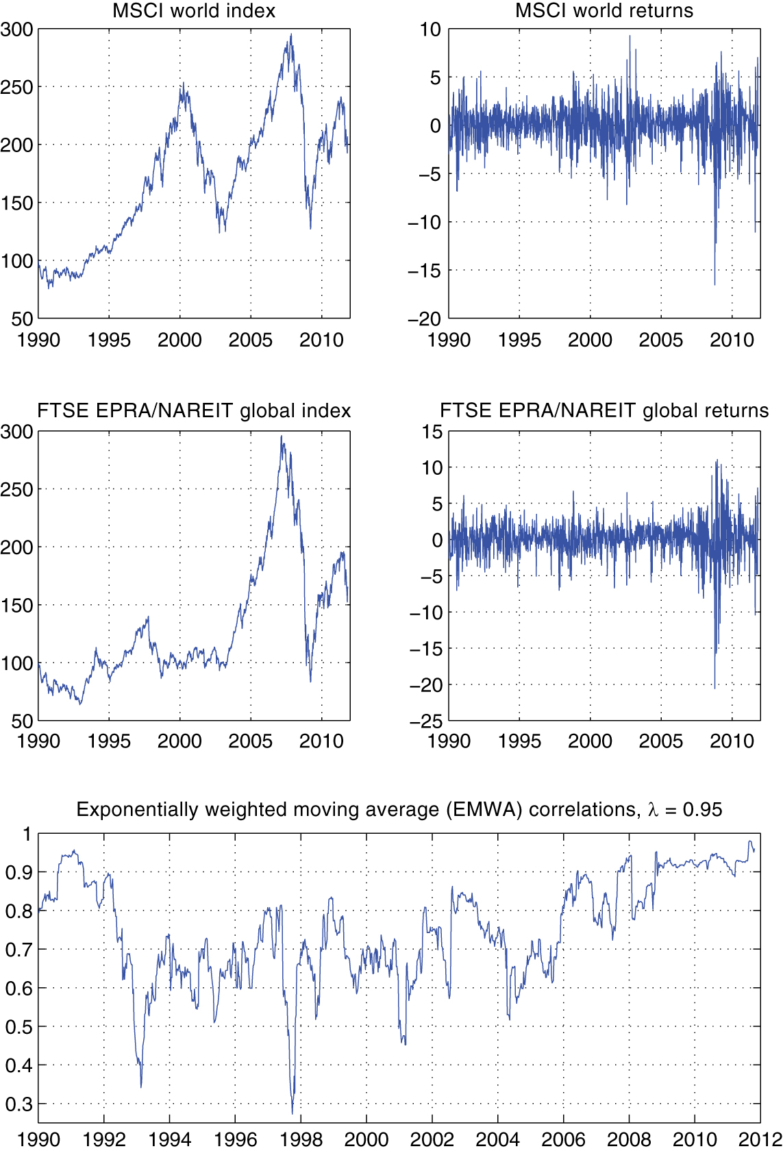
The top panel shows the weekly index levels (left plot) and percentage log returns (right plot) of the MSCI world stock market index from January 1990 to October 2011. The middle panel is similar, but for the FTSE EPRA/NAREIT global index reflecting the evolution of real estate equities. The bottom panel shows conditional correlations implied by an exponentially weighted moving average (EWMA) covariance matrix estimator Ht with smoothing constant λ = 0.95, i.e.
Properties of weekly global stock market and real estate equity returns.
| Mean | Covariance/Correlation matrix | Skewness | Kurtosis | JB | ARCH(10) | ||
|---|---|---|---|---|---|---|---|
| MSCI | 0.064 | 5.077 | 0.795 | −0.762 | 7.49 | 1062.7*** | 175.6*** |
| EPRA/NAREIT | 0.044 | 4.639 | 6.714 | −1.034 | 10.81 | 3091.6*** | 290.0*** |
The top right entry of the “covariance/correlation matrix” is the correlation coefficient, and the bottom left entry is the covariance. The return vector at time t is rt = (r1t, r2t)′, where r1t and r2t are the MSCI and FTSE EPRA/NAREIT returns, respectively, i.e. the first asset is the MSCI world stock index. JB is the Jarque-Bera test for normality, and ARCH(10) is the LM test for ARCH effects with 10 lags (cf. Engle, 1982). Asterisks *** indicate significance at the 1% level.
From Table 1, we note that the return series exhibit a considerable correlation of 0.795, which reflects the common finding that real estate equities display much more similarity to the general stock market than direct real estate investments (e.g. Morawski, Rehkugler & Füss, 2008; Heaney & Sriananthakumar, 2012). Moreover, the bottom panel of Figure 1 shows conditional correlations implied by an exponentially weighted moving average (EWMA) estimator (cf. Alexander, 2008, Ch. 3.8), which hints at time-varying conditional correlations with a particularly strong degree of comovement both at the beginning and the end of the sample, with the latter being also characterized by an outburst of unprecedented volatility.[3] Results for versions of Tse’s (2000) Lagrange Multiplier (LM) test for constant conditional correlations in a multivariate GARCH model are reported in Table 2 and also provide support for time-varying conditional correlations.
| Gaussian innovations | Student’s t innovations | |
|---|---|---|
| test statistic | 7.16*** | 9.84*** |
Reported are the results of Tse’s (2000) Lagrange Multiplier (LM) test for constant conditional correlations under the assumption of both Gaussian (left column) and Student’s t (right column) innovations. Under the null hypothesis, returns are generated by a CCC-AGARCH process as in (25), with k = 1 and (27) imposed in (26). Under the null, the LM test statistic given by (38) has a limiting χ2(1) distribution. Asterisks *** indicate significance at the 1% level.
4.1 Fitting MS CCC-GARCH(1,1) processes
The evidence for time-varying correlations coupled with periods of low and high volatility makes the MS CCC-GARCH model defined in Section 2 a candidate for modeling these series. We fit the model with k = 1, 2, and 3 regimes,[4] where we confine ourselves to the diagonal model, with Aj, Bj, and 𝚪j in (5) being diagonal matrices, j = 1, …, k. In addition, we restrict the asymmetry parameters to be regime-independent, i.e.
There are no clear-cut signs of conditional mean dynamics in the data, and thus we specify the model for return vector rt as
where 𝝁 is the constant conditional mean, and ϵt is generated by an MS(k) CCC-GARCH process as described in Section 2. We compare the fit of models with different k by means of the Bayesian information criterion (BIC) of Schwarz (1978), which, from results of Keribin (2000) and Francq, Roussignol, and Zakoïan (2001), can be expected to have favorable properties for this purpose. Results are reported in Table 3 for both Gaussian and Student’s t innovations {𝝃t} in (3). In both cases, models with two components are preferred, as is a conditional t distribution. Thus we focus on two-component models in the following discussion. Both normal and Student’s t innovations are considered in order to highlight the role of the conditional distribution.
Likelihood-based goodness-of-fit of MS(k) CCC-GARCH models.
| Gaussian innovations | Student’s t innovations | |||||
|---|---|---|---|---|---|---|
| k = 1 | k = 2 | k = 3 | k = 1 | k = 2 | k = 3 | |
| K | 11 | 20 | 31 | 12 | 21 | 32 |
| log L | −4371.5 | −4288.0 | −4261.0 | −4323.7 | −4260.0 | −4247.6 |
| BIC | 8820.4 | 8716.6 | 8740.1 | 8731.7 | 8667.7 | 8720.3 |
Reported are likelihood-based goodness-of-fit measures for diagonal MS(k) CCC-GARCH models fitted to the MSCI world and FTSE EPRA/NAREIT global returns. The number of regimes is denoted by k, and k = 1 corresponds to the single-regime CCC of Bollerslev (1990). In all models, the asymmetry parameters are restricted to be constant across regimes, i.e. in (5), 𝚪1 = ⋯ = 𝚪k. K is the number of parameters of a model, log L is the value of the maximized log-likelihood, and BIC is the Bayesian information criterion of Schwarz (1978), i.e. BIC = −2 × log L + K log T, where T is the sample size. Smaller values of BIC are preferred.
The diagonal MS(k) CCC-GARCH model without further restrictions is rather flexible in that it allows the variances as well as the correlations to be regime-dependent. The contribution of both of these features to the overall improvement over the single-regime specification documented in Table 3 is not clear a priori. It is thus of interest to test various restricted models against the unrestricted specification. Specifically, we consider Pelletier’s (2006) RSDC model where the switching applies to the conditional correlation matrix only, i.e. conditional volatilities are constant across regimes. The second constrained specification represents the opposite of Pelletier’s (2006) model, namely the case where volatility can switch but R1 = R2 in (3). The results reported in Table 4 show that, although both restrictions are rejected against the full model by means of likelihood ratio tests, allowance for regime-specific correlations appears to be more important than switching in the univariate GARCH dynamics, and particularly so for the (generally preferred) models with Student’s t innovations.
Likelihood ratio tests (LRT) of restricted MS(2) CCC-GARCH specifications against the full (diagonal) model
| Gaussian innovations | Student’s t innovations | |||||
|---|---|---|---|---|---|---|
| Full | Pelletier | R1 = R2 | Full | Pelletier | R1 = R2 | |
| (RSDC) | (RSDC) | |||||
| K | 20 | 14 | 19 | 21 | 15 | 20 |
| log L | −4288.0 | −4311.7 | −4313.0 | −4260.0 | −4272.6 | −4310.9 |
| LRT | − | 47.5*** | 50.1*** | − | 25.2*** | 101.9*** |
The table reports likelihood ratio tests (LRT) for restricted versions of the two-component diagonal MS(2) CCC-GARCH model. The unrestricted specification, denoted as “full”, is the model introduced in Section 2 with k = 2, and where the matrices Aj, Bj, j = 1, 2, and 𝚪1 = 𝚪2 in (5) are diagonal. “Pelletier” refers to Pelletier’s (2006) regime-switching dynamic correlation (RSDC) model where only the correlation matrix is subject to regime-switching, i.e. the additional restrictions 𝝎1 = 𝝎2, A1 = A2, and B1 = B2 are imposed in (5). The third model restricts the correlation to be the same in both regimes, i.e. R1 = R2 in (3). log L is the value of the maximized log-likelihood, and K is the number of parameters of a model. The associated likelihood ratio test statistics, denoted as LRT, have 6 and 1 degrees of freedom, respectively. Asterisks *** indicate significance at the 1% level.
Several characteristics of the estimated MS(2) CCC-GARCH models with Gaussian and Student’s t innovations are reported in Table 5, where the single regime CCC-GARCH models are included for comparison. In Table 5, the regimes are ordered such that π1,∞ > π2,∞. Both two-regime models have in common that Regime 1 is a low-volatility regime with moderate correlation (relative to the unconditional correlation), and Regime 2 is a high-volatility regime with rather high correlation, i.e. the diversification potential deteriorates in turbulent market periods. As reported in the bottom part of Table 5, the unconditional moments implied by the single-regime models are close to those of the two-regime specifications and are in between their regime-specific counterparts documented in the top and middle parts of the table for Regimes 1 and 2, respectively. All estimated models are covariance stationary, since
Characteristics of estimated MS CCC-GARCH(1,1) models.
| Estimated characteristic | Gaussian innovations | Student’s t innovations | ||
|---|---|---|---|---|
| k = 1 | k = 2 | k = 1 | k = 2 | |
| ρ12,1 | 0.766 (0.013) | 0.636 (0.025) | 0.769 (0.014) | 0.655 (0.024) |
| 4.265 | 3.691 | 3.847 | 3.161 | |
| 5.528 | 3.540 | 4.713 | 3.318 | |
| 0.754 | 0.617 | 0.756 | 0.636 | |
| p11 | 1 | 0.985 (0.007) | 1 | 0.996 (0.003) |
| π1,∞ | 1 | 0.610 (0.151) | 1 | 0.563 (0.109) |
| ∞ | 66.54a | ∞ | 233.8a | |
| ρ12,2 | – | 0.929 (0.009) | – | 0.921 (0.009) |
| – | 6.080 | – | 5.846 | |
| – | 7.867 | – | 7.785 | |
| – | 0.916 | – | 0.912 | |
| p22 | 0 | 0.976 (0.012) | 0 | 0.994 (0.005) |
| π2,∞ | 0 | 0.390 (0.151) | 0 | 0.437 (0.109) |
| – | 42.49a | – | 181.8a | |
| 4.265 | 4.622 | 3.847 | 4.336 | |
| 5.528 | 5.226 | 4.713 | 5.272 | |
| Corr(ϵ1t, ϵ2t) | 0.754 | 0.779 | 0.756 | 0.805 |
| δ = p11 + p22 − 1 | – | 0.961 (0.017) | – | 0.990 (0.006) |
| ν | – | – | 7.368 (1.025) | 8.584 (1.370) |
| γ11 | 0.680 (0.157) | 0.738 (0.168) | 0.575 (0.181) | 0.627 (0.180) |
| γ22 | 0.401 (0.105) | 0.635 (0.147) | 0.273 (0.116) | 0.472 (0.152) |
| 0.903 | 0.933 | 0.921 | 0.953 | |
Standard errors are given in parentheses. ρ12,j is the constant conditional correlation in Regime j; πj,∞ is the stationary probability and (1 − pjj)−1 is the expected duration of the jth regime, j = 1, 2; δ = p11 + p22 − 1 is a measure for the persistence of the regime process; γ11 and γ22 are the asymmetry parameters in the volatility equation (5) for the MSCI and the FTSE/NAREIT, respectively;
aAsymptotic standard errors for the expected duration of regime j, (1 − pjj)−1, j = 1, 2, could, at least in principle, also be calculated via the delta method. However, with
Comparing the regime-switching models with Gaussian and Student’s t innovations, we observe that both models are characterized by fairly persistent regimes, but the persistence is more pronounced with Student’s t innovations, where both ”staying probabilities” p11 and p22 are rather close to unity. To illustrate the differences in estimated persistence, expected regime durations implied by estimated parameters, given by (1 −
The upper panel of Figure 2 illustrates the models’ inferred switching activity by means of the smoothed regime probabilities of the high-volatility/correlation regime under both types of innovation distribution. Both models indicate a switch to the high-correlation regime at the end of the sample beginning with the financial turmoil in the wake of the burst of the housing bubble. Implications for forecasting are depicted in the lower panel of Figure 2. The left plot of the lower panel of Figure 2 shows conditional correlations as implied by a Gaussian regime-switching model for the two situations where we know for certain that at the forecast origin we are either in the first or second regime.[8] As a function of the forecast horizon, the conditional correlation of the Gaussian model rapidly converges to its unconditional value, whereas forecasts are much more persistently affected by the current state of the world in the Student’s t model, as shown in the bottom right graph of Figure 2.
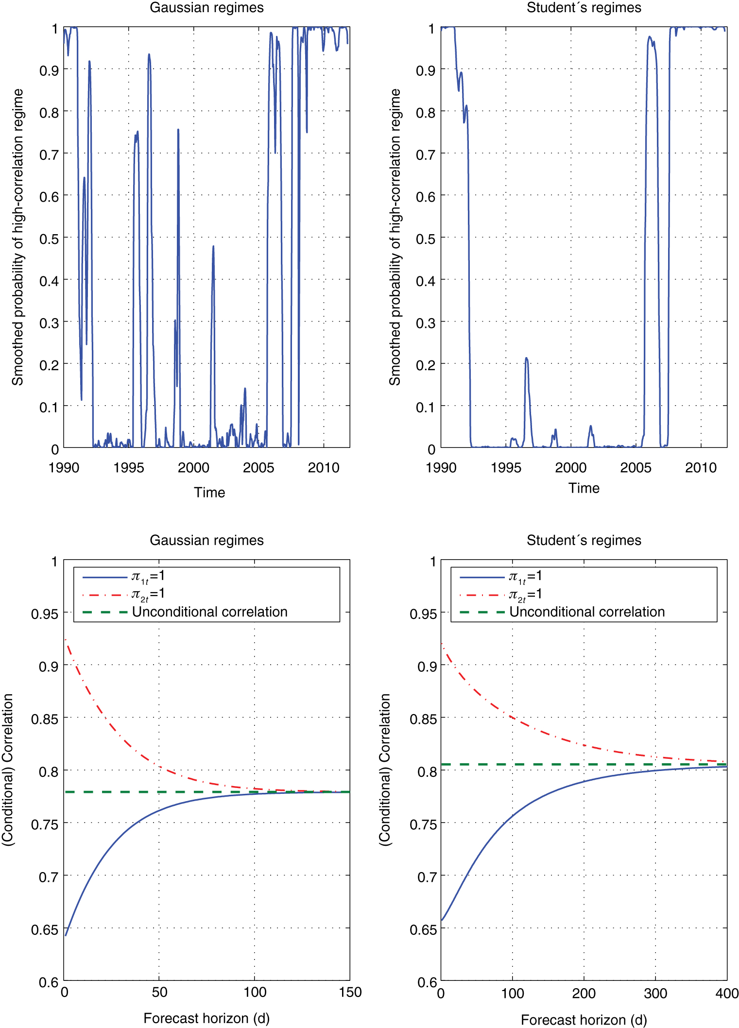
The upper panel shows the smoothed probabilities of Regime 2 (high-volatility/correlation) implied by the MS(2) CCC-GARCH process with Gaussian (left plot) and Student’s t innovations (right plot). The lower panel shows conditional correlations under the assumption that we either start in the low– or high-volatility/correlation regime, as represented by the solid and dash-dotted lines, respectively. Conditional standard deviations have been initialized with appropriate unconditional expectations (cf. Footnote 8). As in the upper panel, the left and right graphs are for Gaussian and Student’s t innovations, respectively.
4.2 Testing for within-regime correlation dynamics and comparison with other models
One of the most popular approaches to time-varying conditional correlations is the dynamic conditional correlation (DCC) model of Engle (2002). In the DCC, conditional correlations are driven by standardized shocks rather than by discrete regime shifts as in the Markov-switching processes studied herein. Both models can be combined to produce an even more flexible structure which allows the conditional correlations in each regime to be driven by DCC-type dynamics (e.g. Billio & Caporin, 2005; Otranto, 2010). However, the MS CCC-GARCH model has several advantages over its DCC-type generalization, since it is easier to estimate and admits the computation of multi-step-ahead conditional covariance matrices. In view of these advantages, it is desirable to have at one’s disposal a simple test of the regime-switching CCC against the alternative of within-regime correlation dynamics. To this end, we extend Tse’s (2000) Lagrange Multiplier (LM) test for constant conditional correlations to the multi-regime framework and allowing for fat-tailed (Student’s t) innovations.[9] The details of this test, which fits into the general framework described by Hamilton (1996), are developed in Appendix C. Results are reported in Table 6 for two conditional volatility specifications under the null hypothesis, that is, both the “full” model from Table 4 as well as Pelletier’s model, and both specifications are considered with Gaussian and Student’s t innovations. Under the alternative, within-regime correlation dynamics are either regime-dependent (case (a) in Table 6) or regime-independent (case (b)). Overall, the results in Table 6 show no clear-cut sign of within-regime correlation dynamics, i.e. the switching between low– and high-correlation periods appears to capture most of the time-variation in conditional correlations.
Lagrange Multiplier (LM) tests for constant within-regime correlations.
| Specification of alternative hypothesis | ||
|---|---|---|
| Case (a) | Case (b) | |
| Gaussian regime densities | ||
| Pelletier (RSDC) | 4.73* | 0.32 |
| MS CCC | 0.46 | 0.33 |
Student’s t regime densities | ||
| Pelletier (RSDC) | 1.46 | 0.12 |
| MS CCC | 4.48 | 0.00 |
Reported are Lagrange Multiplier (LM) tests for constant conditional within-regime correlations in two-regime MS CCC-GARCH models, as described in Appendix C. “Pelletier” is Pelletier’s (2006) regime-switching dynamic correlation (RSDC) model where only the correlation is subject to regime-switching. Note that the tests reported here are based on symmetric volatility processes, i.e. Γ1 = Γ1 = 0 in (5). Cases (a) and (b) are distinguished by means of the alternative hypothesis as described in Appendix C:
Case (a) refers to the situation where, under the alternative, the correlation dynamics may be different in both regimes, i.e. in (26), both δ12,j, j = 1, 2, may be nonzero and different.
In case (b), it is assumed under the alternative that correlation dynamics are regime-independent, i.e. δ12,1 = δ12,2 in (26).
Under the null hypothesis of constant conditional correlations in both regimes, the test statistic for case (a) is asymptotically distributed as χ2(2), whereas in case (b) the limiting distribution is χ2(1). Asterisk * denotes significance at the 10% level (the p–value is 0.094).
In view of these results, we compare conditional correlations implied by the MS CCC and the DCC model of Engle (2002).[10] These correlations are shown in Figure 3 for both Gaussian (top panel) and Student’s t innovations (bottom panel). Comparing the upper with the lower panel of Figure 3, MS CCC-implied correlations are smoother with Student’s t than with Gaussian innovations. The DCC-implied correlations depend much less on the innovation distribution and, as already observed by Pelletier (2006), are less smooth than their regime-switching CCC counterparts.[11] Roughly, however, both types of models contain similar information about low– and high-correlation periods in the data. In particular, they agree with regard to the jump in correlation at the onset of the recent financial crisis.
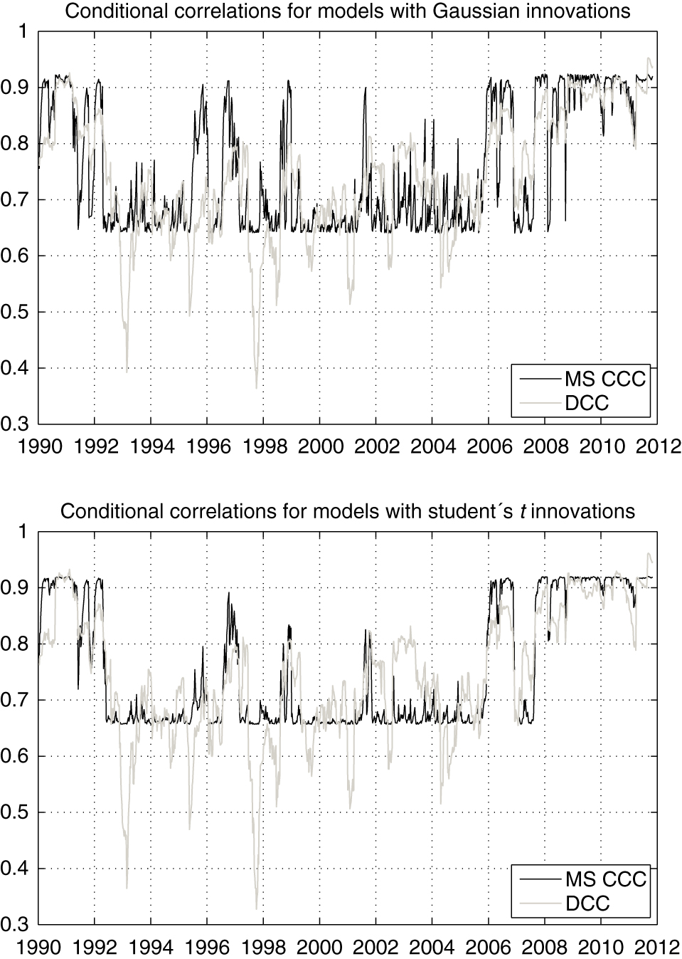
The upper panel shows conditional correlations as implied by the MS CCC-GARCH model and the DCC process with Gaussian innovations. The lower panel repeats this, but for models with Student’s t innovations. The one-step-ahead conditional correlations of the MS CCC-GARCH models are extracted from the conditional covariance matrix (23) for d = 1.
Multi-step ahead conditional correlations for both types of models are illustrated in Figure 4, which resembles the lower part of Figure 3 but additionally includes conditional correlations implied by the Student’s t DCC model, as calculated by simulation.[12] Initial values for the conditional correlation matrix and the conditional standard deviations in the DCC were selected such that they match those of the Student’s t MS CCC in the respective regimes. The long-run correlation of the DCC model is a bit lower than those implied by estimated MS CCC processes. However, with regard to the persistence of multi-step correlations, the DCC is more like the Student’s t rather than the Gaussian MS CCC-GARCH. This is in line with DCC parameter estimates, as reported in Table 7. Interpreting
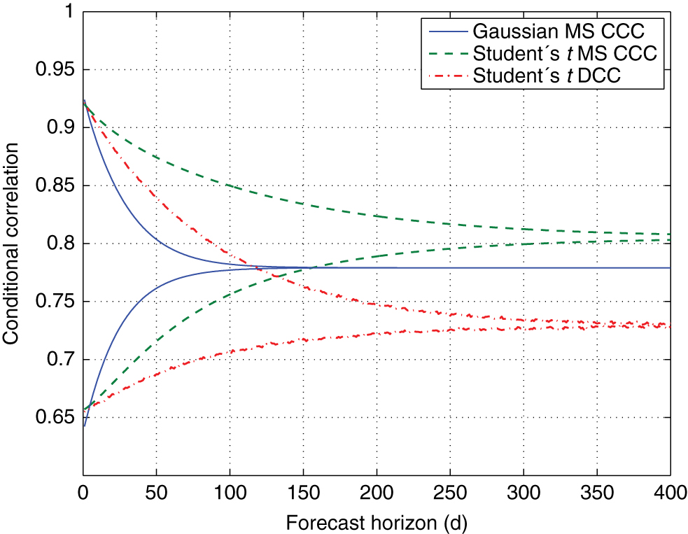
Shown are conditional correlations similar to the lower part of and as explained in the legend of Figure 3. The curves for the MS CCC-GARCH models reproduce those in the bottom part of Figure 3. Initial values for the conditional correlation matrix and the conditional standard deviations in the DCC model were determined such that they match those of the Student’s t MS CCC in the respective (low– and high correlation/variance) regimes.
Parameter estimates for correlation dynamics in DCC models.
| Innovations | |||
|---|---|---|---|
| Gaussian | 0.044 (0.014) | 0.942 (0.022) | 0.986 (0.009) |
| Student’s t | 0.047 (0.015) | 0.941 (0.021) | 0.988 (0.008) |
Shown are estimates of the parameters driving the correlation dynamics in Gaussian and Student’s t DCC models (Engle, 2002), with standard errors given in parentheses. The evolution of the conditional correlation matrix Rt is described by
where the zt are the standardized (“degarched”) residuals, and S is estimated via their sample correlation matrix.
4.3 Application to portfolio selection
We finally compare the models’ performance in an out-of-sample portfolio application. To do so, we first reestimate all models using roughly the first 10 years of data (the first 500 observations) and then update the estimates every 4 weeks, using an expanding window of observations. Estimated models are used to construct ex-ante global minimum variance portfolios (GMVP) over holding periods up to 24 weeks (ca. 6 months).[13] Using non-overlapping holding periods, we thus have, e.g. 637 and 318 out-of-sample realized GMVP returns for the 1– and 2–week holding periods, respectively. Closed-form conditional covariances as derived in Section B.3 are used for all CCC-type models, whereas the DCC-implied conditional covariance matrices are estimated from 10,000 simulated sample paths.
For a broader perspective, we also include three multivariate GARCH models outside of the CCC or DCC families. Namely, we consider the BEKK model of Engle and Kroner (1995) which Gaussian and Student’s t innovations, as well as the multivariate asymmetric mixed normal BEKK-GARCH (MixN BEKK) process of Haas, Mittnik, and Paolella (2009). As detailed in Appendix D, the latter specification combines a conditional mixture distribution with constant mixing weights with conditional regime-specific correlations which are time-varying according to a multivariate BEKK process. Thus the MixN BEKK model can be viewed as the photographic negative of the MS CCC in that the latter’s characteristics of time-varying mixing weights and constant regime-specific correlations have been reversed.
Results are reported in Table 8. For the most basic model, i.e. the single-regime Gaussian CCC, we report the standard deviation of the realized returns, whereas for all other models their respective standard deviation divided by that of the Gaussian CCC is shown. The results in Table 8 show that using a Student’s t rather than a Gaussian distribution improves the results somewhat for all models and forecast horizons. However, the improvements tend to be minor except for the MS CCC-GARCH, for which they are quite substantial, and even more so for longer forecast horizons. At first, it may appear surprising that the MS CCC with Student’s t innovations displays the best results for all forecast horizons, whereas the performance of its Gaussian cousin is rather disappointing. However, this becomes plausible in view of the discussion in Section 4.1. Namely, in the Gaussian model, with volatilities being allowed to switch, the high-volatility regime will tend to latch onto a few “outliers”, which hampers the ability of the model to identify the smooth and long-lived low– and high-correlation regimes. Pelletier’s RSDC model, with switching correlations only, suffers less severely from this problem, and thus its performance is more even across distributional assumptions. Still, however, the results for the MS CCC with t errors in Table 8 suggest that there may be additional benefits from allowing both correlations and volatilities being regime-dependent, provided the conditional distribution is flexible enough to cope with isolated untypical observations within a given regime. Both MS CCC as well as RSDC consistently outperform DCC at longer forecast horizons, which may indicate that the regime-switching models are better suited than the DCC to capture relatively long-lived persistent correlation regimes. On the other hand, however, both the single-regime as well as the MixN BEKK models also improve upon DCC forecasts at longer horizons, suggesting that regime-switching and suitably specified GARCH-type conditional correlations are to some extent substitutes to each other.
Realized standard deviations of out-of-sample global minimum variance portfolio (GMVP) returns.
| Horizon (D) | 1 | 2 | 3 | 4 | 8 | 12 | 16 | 20 | 24 |
|---|---|---|---|---|---|---|---|---|---|
| # returns | 637 | 318 | 212 | 159 | 79 | 53 | 39 | 31 | 26 |
| Conditional correlation models with Gaussian innovations | |||||||||
| CCC | 2.425 | 3.324 | 4.472 | 4.926 | 7.192 | 9.823 | 10.791 | 15.506 | 17.439 |
| DCC | 0.954 | 0.986 | 0.960 | 0.979 | 0.970 | 0.961 | 0.992 | 0.986 | 0.978 |
| RSDC | 0.971 | 0.973 | 0.965 | 0.962 | 0.952 | 0.941 | 0.966 | 0.942 | 0.926 |
| MS CCC | 0.982 | 0.989 | 0.986 | 0.995 | 1.010 | 0.984 | 1.046 | 1.040 | 1.001 |
| Conditional correlation models with Student’s t innovations | |||||||||
| CCC | 0.996 | 0.995 | 0.993 | 0.991 | 0.991 | 0.979 | 0.992 | 0.990 | 0.981 |
| DCC | 0.946 | 0.981 | 0.945 | 0.968 | 0.956 | 0.928 | 0.978 | 0.963 | 0.947 |
| RSDC | 0.961 | 0.968 | 0.951 | 0.953 | 0.935 | 0.901 | 0.952 | 0.924 | 0.895 |
| MS CCC | 0.936 | 0.965 | 0.924 | 0.938 | 0.902 | 0.862 | 0.894 | 0.843 | 0.821 |
| BEKK-type models | |||||||||
| Gaussian BEKK | 0.958 | 1.008 | 0.950 | 0.974 | 0.939 | 0.889 | 0.945 | 0.903 | 0.863 |
| Student’s t BEKK | 0.953 | 0.977 | 0.939 | 0.931 | 0.919 | 0.879 | 0.930 | 0.898 | 0.882 |
| MixN BEKK | 0.960 | 0.964 | 0.948 | 0.941 | 0.943 | 0.907 | 0.938 | 0.889 | 0.867 |
Reported are the results of constructing ex-ante global minimum variance portfolios (GMVP) implied by different GARCH models and for different forecast horizons, D (weeks). Calculations refer to multi-period cumulative returns, i.e. if rt+d is the single-period return vector at time (week) t + d, then the D–period ahead cumulative return vector at forecast origin t is
CCC and DCC are Bollerslev’s (1990) constant and Engle’s (2002) dynamic conditional correlation models, respectively. RSDC is Pelletier’s (2006) model, and MS CCC is the Markov-switching GARCH process defined in Section 2. In all CCC-type and DCC models, volatilities are driven by absolute value asymmetric GARCH processes, cf. Equation (5). BEKK and MixN BEKK are the standard and (two-component) mixed normal BEKK processes, respectively, with asymmetric volatility response as described in Appendix D.
For the CCC with normal innovations, the table reports the standard deviation of the ex-post (realized) portfolio returns of the ex-ante GMVP for each forecast horizon, D. For all other models, their respective standard deviation divided by that of the Gaussian CCC is shown.
5 Concluding remarks
We conclude with a remark referring to the frequently contemplated “curse of dimensionality” problem. An advantage of the (diagonal) CCC, DCC, and Pelletier’s (2006) RSDC models is that, via two-step estimation, application to high-dimensional time series is feasible.[14] This property is not shared by the model studied herein with both regime-specific correlations and variance dynamics. We do not deem this to be a disadvantage, since there are many applications where the advantage of a more flexible dynamic structure may very well outweigh the benefits of parsimony as long as the dimension of the problem is sufficiently low. Studies of the dynamics of broadly defined asset classes, as illustrated in Section 4, are a typical example, where a richer specification can lead to a better understanding and potentially improved forecasts of the joint process under study. As another recent example from the literature somewhat related to the application in Section 4, Case, Guidolin, and Yildrim (2014), using monthly data from 1972 to 2009, find that even a four-regime MS model is required to appropriately describe the evolution of the joint conditional distribution of REIT, stock, and bond returns, since in particular the bond market regimes fail to be synchronized with those of the other two markets. For higher-dimensional systems, Pelletier’s (2006) model, which is nested in the general specification of this paper, appears to provide a reasonable balance between flexibility on the one hand and parsimony and tractability on the other. This is suggested in particular since the results in Section 4 (cf. Table 4) revealed that allowing for regime-switching correlations is of greater value than doing the same for the dynamics of individual volatilities.
Acknowledgements
This paper is a considerably altered version of the manuscript Haas and Liu (2014). The authors are grateful for constructive comments and suggestions from an anonymous referee, which led to significant improvements of the paper. We also thank Jochen Krause, Stefan Mittnik, and participants of the 7th Workshop on Computational and Financial Econometrics in London (CFE 2013), and the annual meeting of the Verein für Socialpolitik 2015 in Münster (Westf.). The research of M. Haas was supported by the Deutsche Forschungsgemeinschaft (HA 5391/2-1). The research of J.-C. Liu was supported by NSF China (11071202, 11301433) and NSF Fujian Province of China (2008J0207).
Appendix
A Proofs of the theorems
Proof of Theorem 1. The ‘if’ part follows from Brandt (1986) or Bougerol and Picard (1992).
Conversely, assume that there exists a strictly stationary solution (ϵt) of the MS(k)-CCC-GARCH process defined by (1)–(6). Iterating (9), we have, for any m > 0, that
From all entries of Xt,
Therefore,
By 𝝎 > 0, this implies
Hence, by Lemma 3.4 in Bougerol and Picard (1992), we know that the top Lyapunov exponent associated with the matrices
Proof of Theorem 2. Write
and Xt,0 = 𝝎. For any vector X such that AX is well defined, we have (AX)⊗l = A⊗lX⊗l. It follows that
By Lemma 1 in Francq and Zakoïan (2005), we have
where
at an exponential rate as m → ∞, because
both in Ll and almost surely. It is obvious that
B Calculation of the moments
We use the notation introduced in Section 3. For later reference, we also define, for j ∈ ℰ,
where 1k is a k–dimensional column of ones.
B.1 The unconditional covariance matrix
For calculating the moments of the MS CCC-GARCH process, we use the following basic result.
Lemma 1
(Francq and Zakoïan (2005), Lemma 3) For ℓ ≥ 1, if the variable Yt−ℓ belongs to the information set generated by {ϵs: s ≤ t − ℓ}, then
where the
Using Lemma 1, we have
Equation (16) implies
where
Thus the first absolute moments are
For the covariance matrix, proceeding similarly,
where C21(j) = 𝝎 ⊗ C1(j) + C1(j) ⊗ 𝝎, j = 1, …, k. Equation (18) implies
where V2 is as V1 in (17) but with πj,∞ E(Xt|Δt−1 = j) replaced by
where definitions (12) and (14) were used. The regime-specific unconditional covariance matrices are also of interest and given by
B.2 Autocorrelations of the absolute process
To calculate the autocorrelation function of the absolute process,
The cross moment matrices are obtained via
where, for i, j = 1, …, k, and with
that is,
where
the diagonal blocks of
For τ = 1, we compute
Hence
where
The expectation in (21) is
where
and
Finally,
and the autocorrelation function can be computed.
B.3 Covariance matrix forecasts
Let 𝝅t = (pt(Δt = 1), …, pt(Δt = k))′ denote the filtered regime probabilities at time t, i.e. the probability distribution of the chain at time t conditional on the history of the process up to time t,[15] and suppose we are given an initial vector Xt+1 (which is known at time t).
Define
so that
Upon repeated substitution in (22), we can write
Let
where, as in (11),
where 𝝅t+d−ℓ = Pd−ℓ𝝅t. Define the matrix
Then the d–step-ahead covariance matrix forecast is given by
Vector
Equations (23) and (24) provide a convenient scheme for calculation of covariance matrix forecasts.
C Lagrange multiplier (LM) test for constant within-regime correlations
The MS-GARCH model with constant within-regime correlations is attractive since it is analytically tractable. E.g. straightforward-to-check conditions for stationarity have been obtained, as well as a simple recursion for calculating multi-step conditional covariance matrices, which is crucial for mean-variance portfolio optimization. Moreover, in some simple cases, such as Pelletier’s (2006) model with regime-independent GARCH dynamics, estimation in high dimensions is feasible via a two-step procedure with an embedded EM algorithm. Despite its convenience, it is still desirable to test whether the assumption of constant within-regime correlation matrices is tenable, since otherwise further improvement of out-of-sample portfolio selection might be feasible by extending the model to allow for within-regime correlation dynamics as in Billio and Caporin (2005) and Otranto (2010). Using results of Hamilton (1996), we extend the Lagrange Multiplier (LM) test devised by Tse (2000) for constant conditional correlations in multivariate GARCH models. In Tse (2000) the LM test is derived under normality of the innovations, but he reports simulations indicating it being quite robust against nonnormality. However, in view of the discussion in Section 4.1, this cannot be expected to hold for MS-GARCH processes, and thus we derive the test allowing for Student’s t errors. The test under normality is then straightforwardly obtained if the degrees of freedom ν → ∞.
For the volatility dynamics, we assume that the conditional standard deviation of asset i in regime j, σijt, is described by a standard (symmetric) AGARCH(1,1) process, i.e. [16]
The conditional correlation matrix in regime j is
where, as in Tse (2000), correlations evolve according to[17]
The null hypothesis of constant conditional within-regime correlations corresponds to
We distinguish between the following cases, which differ in the specification of the alternative hypothesis:
The conditional correlation dynamics are unrestricted across regimes. In this case, under (27), the LM test statistic is asymptotically distributed as χ2 with kM(M − 1)/2 degrees of freedom.
The conditional correlation dynamics are the same across regimes, i.e. δiℓ,1 = δiℓ,2 = ⋯ = δiℓ,k, i = 1, …, M − 1, ℓ = i + 1, …, M. In this case, under (27), the LM test statistic is asymptotically distributed as χ2 with M(M − 1)/2 degrees of freedom.
For the purpose of the current section, it is convenient to decompose the parameter vector of the model as
The log-likelihood of the model for a sample of size T is given by
where
where the squared Mahalanobis distance
with
The regime-specific log-density for observation t is
The partial derivatives of (31) are obtained as
where
where
where
where we initialize all regime-specific conditional standard deviations with the sample standard deviation, i.e. in (34),
The score of the tth observation is given by the derivative of the conditional log-density of
Hamilton (1996) has shown that the derivatives in (35) involving elements of ϑ can be evaluated as
where the second line in (36) is set to zero for t = 1. For τ = t and τ < t, the regime probabilities
Note that, in (36), many terms are zero for parameters that appear in only one regime; e.g. if all parameters except ν are regime-specific, then
For the score with respect to the parameters of P, see Hamilton (1996).[19]
Now let S be the T × N matrix (where N is the dimension of 𝜽) the tth row of which is given by (the transpose of) the score (35), t = 1, …, T, and let
where 1T is a T–dimensional column of ones, and c0 is the number of parameter constraints under H0, see the discussion following Equation (27). Note that the elements of
D The mixed normal BEKK-GARCH (MixN BEKK) model
In this appendix, we briefly describe the mixed normal BEKK-GARCH (MixN BEKK) model applied in Section 4.3, detail the calculation of multi-step-ahead conditional covariance matrices, and discuss a few of its characteristics in comparison with those reported in Table 5.
The asymmetric normal mixture GARCH model in Haas, Mittnik, and Paolella (2009) is an asymmetric extension of the multivariate normal mixture GARCH process of Bauwens, Hafner, and Rombouts (2007).[20] With two mixture components, as in Section 4.3, the conditional distribution of the M–dimensional vector of shocks,
where
where Cj is lower triangular with positive diagonal, j = 1, 2. In line with the other GARCH specifications considered in this paper, the MixN BEKK model used in Section 4.3 imposes the restrictions that
To compute covariance matrix forecasts, write (40) in vech form,
where
In more compact form, (41) can be written as
where
We have[21]
where
with the vector of mixing weights p = (p1, p2)′, and by repeated substitution,
where
and for the cumulative shock,
Bauwens, Hafner, and Rombouts (2007) and Haas, Mittnik, and Paolella (2009) consider the model only with Gaussian mixture components. However, it is clear that, as in (4), a unit-variance Student’s t distribution can be assumed for the mixture components in (39) as well. However, as already reported in Haas, Mittnik, and Paolella (2004a) for daily stock returns and confirmed for our data, use of fat-tailed component densities typically does not lead to significant improvements in this kind of model. This is in sharp contrast to the Markov-switching models investigated herein and thus may appear a bit surprising at first glance. It can be explained by the fact that, in contrast to the Markov-switching process (with time-varying conditional regime probabilities), the independent switching process of the MixN BEKK model as such does not add to the dynamics of the conditional moment structure. Rather, the conditional mixed normal distribution in (39) mainly contributes to conditional leptokurticity and thus essentially serves the same purpose as a conditional Student’s t distribution. As conditional mixed normality is often sufficient to capture the excess kurtosis in the data, the degrees of freedom parameter in t–mixture GARCH models tends to be somewhat ill-identified and unstable and erratic over time. We have observed the same phenomenon for our data and thus only use the Gaussian mixture GARCH in Section 4.3.
To illustrate, we briefly compare the parameter estimates over the entire sample as reported in Table 5 with those from the two-component MixN BEKK model, as shown in Table 9. Table 9 reports the estimated mixing weights p1 and p2 = 1 − p1 as well as the unconditional component-specific variances and correlations implied by the estimated parameters. Comparing the results in Table 9 with those for the MS CCC models in Table 8, the following differences can be observed. First, in the MixN BEKK model, the correlation is essentially regime-independent. This can be explained by the fact that, in the MixN BEKK model, conditional correlations are driven by the BEKK dynamics for the component covariance matrices, whereas the (independent) switching process mainly accounts for the conditional leptokurtosis. The kurtosis of a two-component normal mixture distribution is particularly large when there are sizeable differences between the component variances and the mixing weight of the high-variance regime is small (cf. Timmermann, 2000). The differences in volatility between the regimes are more pronounced in the MixN BEKK process,[22] and the mixing weight of its high-volatility component is p2 = 0.126, which is about one third of the unconditional high-volatility regime probability π2,∞ = 0.390 in the Gaussian MS CCC model.
Characteristics of the estimated MixN BEKK model.
| Corr(ϵ1t, ϵ2t|Δt = 1) | p1 | ||
| 3.133 | 3.713 | 0.730 | 0.874 (0.031) |
| p2 | |||
| 10.16 | 14.89 | 0.718 | 0.126 (0.031) |
Due to the independent switching,
References
Abramson, A., and I. Cohen. 2007. “On the Stationarity of Markov-Switching GARCH Processes.” Econometric Theory 23: 485–500.10.1017/S0266466607070211Search in Google Scholar
Alexander, C. 2008. Practical Financial Econometrics. Chichester: John Wiley & Sons.Search in Google Scholar
Alexander, C., and E. Lazar. 2006. “Normal Mixture GARCH(1,1). Applications to Exchange Rate Modelling.” Journal of Applied Econometrics 21: 307–336.10.1002/jae.849Search in Google Scholar
Alexander, C., and E. Lazar. 2009. “Modelling Regime-Specific Stock Price Volatility.” Oxford Bulletin of Economics and Statistics 71: 761–797.10.1111/j.1468-0084.2009.00563.xSearch in Google Scholar
Ang, A., and A. Timmermann. 2012. “Regime Changes and Financial Markets.” Annual Review of Financial Economics 4: 313–337.10.3386/w17182Search in Google Scholar
Ardia, D. 2009. “Bayesian Estimation of a Markov-Switching Threshold Asymmetric GARCH Model with Student-t Innovations.” Econometrics Journal 12: 105–126.10.1111/j.1368-423X.2008.00253.xSearch in Google Scholar
Augustyniak, M. 2014. “Maximum Likelihood Estimation of the Markov-Switching GARCH Model.” Computational Statistics and Data Analysis 76: 61–75.10.1016/j.csda.2013.01.026Search in Google Scholar
Bauwens, L., C. M. Hafner, and J. V. K. Rombouts. 2007. “Multivariate Mixed Normal Conditional Heteroskedasticity.” Computational Statistics and Data Analysis 51: 3551–3566.10.1016/j.csda.2006.10.012Search in Google Scholar
Billio, M., and M. Caporin. 2005. “Multivariate Markov Switching Dynamic Conditional Correlation GARCH Representations for Contagion Analysis.” Statistical Methods & Applications 14: 145–161.10.1007/s10260-005-0108-8Search in Google Scholar
Bollerslev, T. 1990. “Modelling the Coherence in Short-Run Nominal Exchange Rates: A Multivariate Generalized ARCH Model.” Review of Economics and Statistics 73: 498–505.10.2307/2109358Search in Google Scholar
Bougerol, P., and N. Picard. 1992. “Strict Stationarity of Generalized Autoregressive Processes.” Annals of Probability 20: 1714–1730.10.1214/aop/1176989526Search in Google Scholar
Brandt, A.. 1986. “The Stochastic Equation Yn+1 = An Yn + Bn with Stationary Coefficients.” Advances in Applied Probability 18: 211–220.10.1017/S0001867800015639Search in Google Scholar
Broda, S. A., M. Haas, J. Krause, M. S. Paolella, and S. C. Steude. 2013. “Stable Mixture GARCH Models.” Journal of Econometrics 172: 292–306.10.1016/j.jeconom.2012.08.012Search in Google Scholar
Bulla, J. 2011. “Hidden Markov Models with t Components. Increased Persistence and Other Aspects.” Quantitative Finance 11: 459–475.10.1080/14697681003685563Search in Google Scholar
Campbell, R., K. Koedijk, and P. Kofman. 2002. “Increased Correlation in Bear Markets: A Downside Risk Perspective.” Financial Analysts Journal 58: 87–94.10.2469/faj.v58.n1.2512Search in Google Scholar
Case, B., M. Guidolin, and Y. Yildrim. 2014. “Markov Switching Dynamics in Reit Returns: Univariate and Multivariate Evidence on Forecasting Performance.” Real Estate Economics 42: 279–342.10.1111/1540-6229.12025Search in Google Scholar
Conrad, C. and M. Karanasos. 2010. “Negative Volatility Spillovers in the Unrestricted ECCC-GARCH Model.” Econometric Theory 26: 838–862.10.1017/S0266466609990120Search in Google Scholar
Conrad, C., and M. Karanasos. 2015. “Modeling the Link between us Inflation and Output: The Importance of the Uncertainty Channel.” Scottish Journal of Political Economy 62: 431–453.10.2139/ssrn.1715088Search in Google Scholar
Dean, W. G., and R. W. Faff. 2008. “Evidence of Feedback Trading with Markov Switching Regimes.” Review of Quantitative Finance and Accounting 30: 133–151.10.1007/s11156-007-0047-6Search in Google Scholar
Ding, Z., C. W. J. Granger, and R. F. Engle (1993): “A Long Memory Property of Stock Market Returns and a New Model.” Journal of Empirical Finance 1: 83–106.10.1016/0927-5398(93)90006-DSearch in Google Scholar
Dueker, M. J. 1997. “Markov Switching in GARCH Processes and Mean-Reverting Stock-Market Volatility.” Journal of Business and Economic Statistics 15: 26–34.10.20955/wp.1994.015Search in Google Scholar
Engle, R. F. 1982. “Autoregressive Conditional Heteroscedasticity with Estimates of the Variance of united kingdom Inflation.” Econometrica 50: 987–1008.10.2307/1912773Search in Google Scholar
Engle, R. F. 2002. “Dynamic Conditional Correlation: A Simple Class of Multivariate Generalized Autoregressive Conditional Heteroskedasticity Models.” Journal of Business and Economic Statistics 20: 339–350.10.1198/073500102288618487Search in Google Scholar
Engle, R. F., and K. F. Kroner. 1995. “Multivariate Simultaneous Generalized ARCH.” Econometric Theory 11: 122–150.10.1017/S0266466600009063Search in Google Scholar
Francq, C., and J.-M. Zakoïan. 2005. “The l2–Structures of Standard and Switching-Regime GARCH Models.” Stochastic Processes and their Applications 115: 1557–1582.10.1016/j.spa.2005.04.005Search in Google Scholar
Francq, C., and J.-M. Zakoïan. 2012. “Qml Estimation of a Class of Multivariate Asymmetric GARCH Models.” Econometric Theory 28: 179–206.10.1017/S0266466611000156Search in Google Scholar
Francq, C., M. Roussignol, and J.-M. Zakoïan. 2001. “Conditional Heteroskedasticity Driven by Hidden Markov Chains.” Journal of Time Series Analysis 22: 197–220.10.1111/1467-9892.00219Search in Google Scholar
Giot, P., and S. Laurent. 2003. “Value-at-Risk for Long and Short Trading Positions.” Journal of Applied Econometrics 18: 641–664.10.1002/jae.710Search in Google Scholar
Glosten, L. R., R. Jagannathan, and D. E. Runkle. 1993. “On the Relation between the Expected Value and the Volatility of the Nominal Excess Return on Stocks.” Journal of Finance 48: 1779–1801.10.1111/j.1540-6261.1993.tb05128.xSearch in Google Scholar
Gray, S. F. 1996. “Modeling the Conditional Distribution of Interest Rates as a Regime-Switching Process.” Journal of Financial Economics 42: 27–62.10.1016/0304-405X(96)00875-6Search in Google Scholar
Gribisch, B. 2016. “Multivariate Wishart Stochastic Volatility and Changes in Regime.” AStA - Advances in Statistical Analysis 100: 443–473.10.1007/s10182-016-0269-9Search in Google Scholar
Guidolin, M. 2011. “Markov Switching Models in Empirical Finance.” In Missing Data Methods: Time-Series Methods and Applications (Advances in Econometrics, Volume 27), edited by D. M. Drukker, 1–86. Bingley: Emerald.10.1108/S0731-9053(2011)000027B004Search in Google Scholar
Haas, M. 2010. “Covariance Forecasts and Long-Run Correlations in a Markov-Switching Model for Dynamic Correlations.” Finance Research Letters 7: 86–97.10.1016/j.frl.2009.12.002Search in Google Scholar
Haas, M., and J.-C. Liu. 2014. “Theory for a Multivariate Markov-Switching GARCH Model with an Application to Stock Markets.” QBER Discussion Paper 7/2014, University of Kiel.Search in Google Scholar
Haas, M., S. Mittnik, and M. S. Paolella. 2004a. “Mixed Normal Conditional Heteroskedasticity.” Journal of Financial Econometrics 2: 211–250.10.1093/jjfinec/nbh009Search in Google Scholar
Haas, M., S. Mittnik, and M. S. Paolella. 2004b. “A New Approach to Markov-Switching GARCH Models.” Journal of Financial Econometrics 2: 493–530.10.1093/jjfinec/nbh020Search in Google Scholar
Haas, M., S. Mittnik, and M. S. Paolella. 2009. “Asymmetric Multivariate Normal Mixture GARCH.” Computational Statistics and Data Analysis 53: 2129–2154.10.1016/j.csda.2007.12.018Search in Google Scholar
Haas, M., and M. S. Paolella. 2012. “Mixture and Regime-Switching GARCH Models.” In Handbook of Volatility Models and their Applications, edited by L. Bauwens, C. M. Hafner, and S. Laurent. John Wiley & Sons.10.1002/9781118272039.ch3Search in Google Scholar
Hamilton, J. D. 1994. Time Series Analysis. Princeton, New Jersey: Princeton University Press.10.1515/9780691218632Search in Google Scholar
Hamilton, J. D. 1996. “Specification Testing in Markov-Switching Time-Series Models.” Journal of Econometrics 70: 127–157.10.1016/0304-4076(69)41686-9Search in Google Scholar
He, C., and T. Teräsvirta. 2004. “An Extended Constant Correlation GARCH Model and its Fourth-Moment Structure.” Econometric Theory 20: 904–926.10.1017/S0266466604205059Search in Google Scholar
Heaney, R., and S. Sriananthakumar. 2012. “Time-Varying Correlation between Stock Market Returns and Real Estate Returns.” Journal of Empirical Finance 19: 583–594.10.1016/j.jempfin.2012.03.006Search in Google Scholar
Jeantheau, T. 1998. “Strong Consistency of Estimators for Multivariate ARCH Models.” Econometric Theory 14: 70–86.10.1017/S0266466698141038Search in Google Scholar
Jondeau, E., and M. Rockinger. 2006. “The Copula-GARCH Model of Conditional Dependencies: An International Stock Market Application.” Journal of International Money and Finance 25: 827–853.10.1016/j.jimonfin.2006.04.007Search in Google Scholar
Kasch, M., and M. Caporin. 2013. “Volatility Threshold Dynamic Conditional Correlations: An International Analysis.” Journal of Financial Econometrics 11: 706–742.10.1093/jjfinec/nbs028Search in Google Scholar
Keribin, C. 2000. “Consistent Estimation of the Order of Mixture Models.” Sankhyā: The Indian Journal of Statistics, Series A 62: 49–66.Search in Google Scholar
Kim, C.-J., and C. R. Nelson. 1999. State-Space Models with Regime Switching. Cambridge, Massachusetts: MIT Press.Search in Google Scholar
Klaassen, F. 2002. “Improving GARCH Volatility Forecasts with Regime-Switching GARCH.” Empirical Economics 27: 363–394.10.1007/978-3-642-51182-0_10Search in Google Scholar
Ledoit, O., P. Santa-Clara, and M. Wolf. 2003. “Flexible Multivariate GARCH Modeling with an Application to International Stock Markets.” Review of Economics and Statistics 85: 735–747.10.1162/003465303322369858Search in Google Scholar
Lee, Y.-H. 2014. “An International Analysis of REITs and Stock Portfolio Management based on Dynamic Conditional Correlation Models.” Financial Markets and Portfolio Management 28: 165–180.10.1007/s11408-014-0227-zSearch in Google Scholar
Lejeune, B. 2009. “A Diagnostic m-test for Distributional Specification of Parametric Conditional Heteroscedasticity Models for Financial Data.” Journal of Empirical Finance 16: 507–523.10.1016/j.jempfin.2008.11.005Search in Google Scholar
Liu, J.-C. 2006. “Stationarity of a Markov-Switching GARCH Model.” Journal of Financial Econometrics 4: 573–593.10.1093/jjfinec/nbl004Search in Google Scholar
Liu, J.-C. 2007. “Stationarity for a Markov-Switching Box-Cox Transformed Threshold GARCH Process.” Statistics and Probability Letters 77: 1428–1438.10.1016/j.spl.2007.02.009Search in Google Scholar
Magnus, J. R. 1988. Linear Structures. London: Griffin.Search in Google Scholar
Manner, H., and O. Reznikova. 2012. “A Survey on Time-Varying Copulas: Specification, Simulations, and Application.” Econometric Reviews 31: 654–687.10.1080/07474938.2011.608042Search in Google Scholar
McAleer, M., S. Hoti, and F. Chan. 2009. “Structure and Asymptotic Theory for Multivariate Asymmetric Conditional Volatility.” Econometric Reviews 28: 422–440.10.1080/07474930802467217Search in Google Scholar
Mittnik, S. 2014. “Var-Implied Tail-Correlation Matrices.” Economics Letters 122: 69–73.10.1016/j.econlet.2013.10.025Search in Google Scholar
Morawski, J., H. Rehkugler, and R. Füss. 2008. “The Nature of Listed Real Estate Companies: Property or Equity Market?” Financial Markets and Portfolio Management 22: 101–126.10.1007/s11408-008-0075-9Search in Google Scholar
Nabeya, S. 1951. “Absolute Moments in 2-Dimensional Normal Distribution.” Annals of the Institute of Statistical Mathematics 3: 2–6.10.1007/BF02949771Search in Google Scholar
Nakatani, T., and T. Teräsvirta. 2008. “Positivity Constraints on the Conditional Variances in the Family of Conditional Correlation GARCH Models.” Finance Research Letters 5: 88–95.10.1016/j.frl.2008.02.001Search in Google Scholar
Nakatani, T., and T. Teräsvirta. 2009. “Testing for Volatility Interactions in the Constant Conditional Correlation GARCH Model.” Econometrics Journal 12: 147–163.10.1111/j.1368-423X.2008.00261.xSearch in Google Scholar
Otranto, E. 2010. “Asset Allocation using Flexible Dynamic Correlation Models with Regime Switching.” Quantitative Finance 10: 325–338.10.1080/14697680902856515Search in Google Scholar
Pelletier, D. 2006. “Regime Switching for Dynamic Correlations.” Journal of Econometrics 131: 445–473.10.1016/j.jeconom.2005.01.013Search in Google Scholar
Putintseva, M. 2012. “Mixture Normal Conditional Correlation Models.” Research Paper No. 12-41, Swiss Finance Institute.Search in Google Scholar
Ramchand, L., and R. Susmel. 1998. “Volatility and Cross Correlation Across Major Stock Markets.” Journal of Empirical Finance 5: 397–416.10.1016/S0927-5398(98)00003-6Search in Google Scholar
Reher, G., and B. Wilfling. 2016. “A Nesting Framework for Markov-Switching GARCH Modelling with an Application to the German Stock Market.” Quantitative Finance 16: 411–426.10.1080/14697688.2015.1015599Search in Google Scholar
Ryden, T., T. Teräsvirta, and S. Åsbrink. 1998. “Stylized Facts of Daily Return Series and the Hidden Markov Model.” Journal of Applied Econometrics 13: 217–244.10.1002/(SICI)1099-1255(199805/06)13:3<217::AID-JAE476>3.0.CO;2-VSearch in Google Scholar
Schwarz, G. 1978. “Estimating the Dimension of a Model.” Annals of Statistics 6: 461–464.10.1214/aos/1176344136Search in Google Scholar
Shi, Y., and L. Feng. 2016. “A Discussion on the Innovation Distribution of the Markov Regime-Switching GARCH Model.” Economic Modelling 53: 278–288.10.1016/j.econmod.2015.11.018Search in Google Scholar
Silvennoinen, A., and T. Teräsvirta. 2009a. “Modeling Multivariate Autoregressive Conditional Heteroskedasticity with the Double Smooth Transition Conditional Correlation GARCH Model.” Journal of Financial Econometrics 7: 373–411.10.1093/jjfinec/nbp013Search in Google Scholar
Silvennoinen, A., and T. Teräsvirta. 2009b. “Multivariate GARCH Models.” In Handbook of Financial Time Series, edited by T. Mikosch, J.-P. Kreiß, R. A. Davis, and T. G. Andersen, 201–229. Berlin: Springer.10.1007/978-3-540-71297-8_9Search in Google Scholar
Smith, D. R. 2008. “Evaluating Specification Tests for Markov-Switching Time-Series Models.” Journal of Time Series Analysis 29: 629–652.10.1111/j.1467-9892.2008.00575.xSearch in Google Scholar
Taylor, S. J. 1986. Modelling Financial Time Series. Chichester: John Wiley & Sons.Search in Google Scholar
Timmermann, A. 2000. “Moments of Markov Switching Models.” Journal of Econometrics 96: 75–111.10.1016/S0304-4076(99)00051-2Search in Google Scholar
Tse, Y. K. 2000. “A Test for Constant Correlations in a Multivariate GARCH Model.” Journal of Econometrics 98: 107–127.10.1016/S0304-4076(99)00080-9Search in Google Scholar
Supplemental Material
The online version of this article offers supplementary material (DOI: https://doi.org/10.1515/snde-2016-0019).
Code and Datasets
The author(s) published code and data associated with this article is on Code Ocean, a computational reproducibility platform. We recommend Code Ocean to SNDE contributors who wish share, discover, and run code in published research articles. (See: https://doi.org/10.24433/CO.2bf91781-8f40-4e16-89bb-35c7ce77f43e).
©2018 Walter de Gruyter GmbH, Berlin/Boston