
Abstract
The current game theory model method cannot accurately optimize the load control of smart grid, resulting in the problem of high load energy consumption when the smart grid is running. To address this problem, a load optimal control algorithm for smart grid based on demand response in different scenarios is proposed in this paper. The demand response of smart grid under different scenarios is described. Onthis basis, the load rate and actual load of smart grid are calculated by using the rated load of electrical appliances. The load classification of smart grid and the main factors affecting the load of smart grid are analyzed to complete the load distribution of smart grid. According to the evaluation function of smart grid, the number of load clusters is adjusted to calculate the load change rate. The trend of load curve of smart grid is analyzed to realize optimal load control of smart grid under different scenarios. The experimental results show that the proposed method has better control performance and higher accuracy through load control of smart grid.
1 Introduction
With the development of human society, the demand for energy, especially electric energy, is increasing. Smart grid plays an important role in the task of transmitting electric energy [1]. The continuous advancement of the process of electricity market and the continuous improvement of the power reliability and quality requirements of the users require that the smart grid must be able to provide safer, reliable, clean, and high quality power supply. In order to solve the bottleneck problem of smart grid development, scholars at home and abroad have made active exploration and carried out research on smart grid [2]. Through a digital information network system, energy resources are connected to various electrical and other energy utilities of energy end users. Through intelligent control, accurate energy supply, corresponding energy supply, mutual aid energy supply and complementary energy supply are realized, and energy utilization efficiency and energy supply security are raised to a new level, which makes user cost and investment benefit attain a reasonable state. Because the research and development of the smart grid is still in its infancy, and the national conditions and the distribution of resources are different, the direction and emphasis of the development of smart grid are not the same. In fact, there is no uniform and definitive definition [3]. From the perspective of technology development and application, experts and scholars from different countries and regions generally agree with the following viewpoint. The load optimization control of smart grid is to optimize and control the load generated by the smart grid when it is running. The advanced sensing and measurement technology, information and communication technology, analysis and decision-making technology, automatic control technology, and energy and power technology are combined. A new modern power grid is formed, which is highly integrated with smart grid infrastructure. Smart grid will be a new type of power grid combined with power network and information network. Load will inevitably occur when the power grid is running, so the research on load optimization control of smart grid under different scenarios will become an important research direction.
In the literature [4], a cluster based evolutionary algorithm for optimal load control of smart grid under different scenarios is proposed. Using cluster analysis, certain structural connection between individuals of evolving smart grid is constructed. The virtual cluster based organization is used to coordinate and control the calculation process of smart grid load optimization. The solution of the higher load of the smart grid when running is calculated, and the best solution is obtained. However, the algorithm has the problem of high energy consumption control, which cannot operate safely and steadily, shorten the service life of the unit, and cannot effectively control the load of the smart grid. In the literature [5], a load optimal control algorithm for smart grid under different scenarios is proposed based on chaotic particle swarm optimization. The smart grid’s valve point effect and load constraint conditions are analyzed. A penalty function mathematical model for load distribution optimization of smart grid is built. Chaotic particle swarm optimization algorithm is introduced to calculate the voltage and current of smart grid. The influence of voltage and current on the load of smart grid is analyzed, and the load optimization control of smart grid is realized. However, the algorithm has high energy consumption control and poor control performance. In the literature [6], a load optimal control algorithm for smart grid under different scenarios is proposed based on improved neural network algorithm. A mathematical model for the operation of smart grid is built. Using the principle of reducing dimension, the matrix and original matrix information of smart grid after dimension reduction are calculated, and the load generated by smart grid operation is obtained. Combined with the mathematical model and matrix information of smart grid, the load optimization control is completed. However, this method has the disadvantages of low load control performance, poor control efficiency and low precision of smart grid. In the literature [7], a load optimal control algorithm based on improved immune clonal selection algorithm for smart grid under different scenarios is proposed. A multi-objective optimization control model for smart grid load is built. The load is applied to the demand response process of time-of-use price, and the optimal control of smart grid load is realized. However, this method has a low precision.
In demand response, pricing strategy, as part of demand response, has its irreplaceable importance. Demand response in many cases is by means of price. The adjustment of electricity prices or incentives to achieve regulation and control has attracted considerable attention. In the demand response of smart grid, the interaction between power supply and power consumption is not obvious, which leads to the difficulty of the demand response mechanism in the smart grid. Smart grid integrates advanced information, control and communication technologies to provide strong technical support for the successful implementation of demand response mechanism. In this paper, a load optimal control algorithm for smart grid based on demand response in different scenarios is proposed. The framework of the research is given as follows.
The demand response of smart grid in different scenarios is described, and the price demand response and incentive demand response of smart grid are analyzed. The actual load of smart grid is calculated and the load of smart grid is classified. The main factors that affect the power load of the smart grid are analyzed, and the lighting load of the smart grid is calculated to complete the distribution of smart grid load in different scenes.
By adjusting the evaluation function to adjust the clustering number of smart grid data, the optimal clustering number can be obtained. The changing trend of the load curve of the smart grid is analyzed. The demand response of smart grid is introduced to realize optimal load control of smart grid under different scenarios.
By analyzing the operation data of smart grid, the efficiency of data in smart grid is compared. The comparison of the load generated by smart grid operation is carried out. The effectiveness of the proposed method is proved.
The conclusions of the research.
2 Methods
2.1 Demand response of smart grid in different scenarios
Demand response refers to the end-users’ initiative to change their normal electricity consumption behavior according to market information (price signal or incentive mechanism provided by operators), which promotes market stability and power reliability. The demand response of smart grid in different scenarios can be divided into two categories: price demand response and incentive demand response, as shown in Figure 1
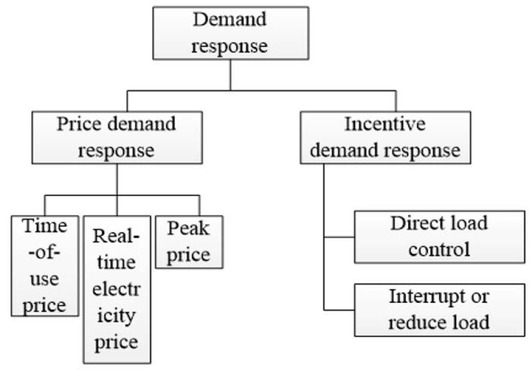
Demand response of smart grid in different scenarios
Price demand response refers to the retail market price at which the end-user directly faces the wholesale market or is linked to the wholesale market price and change the way of consumption or behavior of electricity consumption by responding to price signals. Finally, it is to reduce the cost of their own electricity consumption, improve the efficient use of smart grid resources, postpone the new amount of investment, and ensure the stability and security of the smart grid. In the response to the price demand, users automatically adjust their electricity consumption according to the time changing tariff, such as time sharing price, real time electricity price and peak price [8]. Users who use this tariff can reduce the electricity fee by adjusting the power consumption time (at lower electricity prices and lower electricity consumption at higher prices).
Time-of-use (TOU) price: Electricity price fluctuates within 24 hours of a day, but it is fixed within a specified period of time. TOU price reflects the average cost of generation and transmission in the corresponding period. TOU price can be changed according to the different seasons of the day (such as peak and non-peak period), according to different seasons, and it is decided by several months or even years in advance. TOU price is widely used by large commercial and industrial users and require meters to store accumulated electricity consumption over different periods of time [9].
Spot price: This is an idealized instantaneous dynamic pricing policy. In practice, electricity prices usually change at an hourly basis. Spot price reflects changes in power generation costs and wholesale prices of power plants. Spot price is usually provided to the user one day or one hour in advance, so that the user can plan the electricity consumption ahead of schedule. However, the use of spot price increases the cost of installing communication equipment and control equipment.
Peak price: In the power system, the severe peak load caused by the weather and the state of the system rarely occurs, and it will cause a great threat to the entire grid system once it occurs. Peak price is another dynamic pricing mechanism which is eliminated by combining spot price and TOU price. It is derived from the peak load rate on the TOU price, which can reflect the short term market power supply cost.
Incentive demand response is further divided into classical solution and market-based solution. The classic incentive demand response includes direct load control and interruptible or reduced load. In the classic incentive demand response, the participating users receive the participation fee, which can usually be used as the account amount or discount rate of the programs they participate in [10]. In a market-based scenario, participants are rewarded with money based on their performance, depending on the amount of load reduction under critical circumstances. Load is divided into direct load control and interruptible load.
Direct load control: It refers to the remote shutdown or cycle operation of the user’s electrical equipment in a short time, such as air conditioner or hot water. Direct load control scheme is mainly used to ensure the reliability of smart grid operation when the power price fluctuates greatly. Usually, direct load control is mainly for residential users or small business users.
Interruptible (or reduced) load: It is to integrate the option of reducing service into the retail price, and the power operator can offer a price discount to the user or reduce the electricity price directly to the user. Users must agree to reduce power consumption when there is an emergency in the power system. Unlike direct load control, interruptible loads are typically designed for the largest industrial and commercial customers [11]. Customers may face penalties if they violate the terms of the agreement and fail to cut their electricity load.
2.2 Load distribution in smart grid
In the smart grid with different scenarios, the electricity demand of residential users affects the formulation of the electric power production plan. The demand of residential users depends on three factors: the number of appliances, the power of appliances, and the use of appliances. The use of electrical appliances is determined by user behavior. The factors affecting the use of electrical appliances are the most complex and unpredictable [12]. In the study of the conversion model between the user’s electricity consumption behavior and the power demand, the power demand level varies between different users and different times due to the user’s electrical behavior and time.
Assume in different scenarios, the resident user is a family composed of s members. The set of activities of members can be represented as
Where xj(t) ∈ X is the activity of the jth person at the t time, X is the activity set. The activities of each member of a resident user in different scenarios have temporal attributes, which can be deterministic or random and uncertain. For this uncertainty, Markoff chain can be used to describe it. For the activity of the jth individual, the transition probability can be represented by the function pj : X × X → [0, 1]. pj(xj(t), xj(t + 1)) is the probability of the individual transiting from t time activity xj(t) to t + 1 time activity xj(t + 1), which satisfies
All kinds of activities required by residents need to use one or more electrical equipment [13]. Different activities use different ways of electrical appliances. σ denotes load rate of different electrical appliances for different activities [14]. Assume σ : X × E → [0, 1] is the electrical load mapping in smart grid, σ(x, e) is the load rate of the appliance e under the activity x, σ(x, e)pe is the actual load of the appliance e under the activity x, pe is the rated load of electrical appliance. Deterministic user power consumption behavior is {xj(t) : j = 1, 2, ..., s}, the load rate δ(t, e) of the appliance e at the t time and the actual load of smart grid user p(t) are given by
Where
2.2.1 Load classification of smart grid
Electric load of smart grid in different scenarios can be divided into kitchen electricity, bedroom electricity, bathroom electricity and living room electricity according to regional division. According to user behavior, electricity consumption can be divided into three main categories: going to work, dining, entertainment and leisure, and household electricity consumption. The electrical appliances involved include electric lamp, television, computer, air conditioner, rice cooker, induction cooker, refrigerator and washing machine [17]. With the continuous increase of the income level of residents, the consumption of recreational and residential electricity is increasing. During the peak period, the power transmission of smart grid across the country is facing great challenges. It has become an important problem in load control range of smart grid to enable resident users to use electricity spontaneously and consciously by avoiding peak load and staggering peak load. The living electricity of urban residents has changed from the lighting power to the refrigerator and air conditioning, which has a significant impact on the planning and design of the load classification and the safe and economical operation of the smart grid.
2.2.2 Main factors affecting the power consumption of smart grid
The power load of the smart grid includes the electric load of the bedroom, the load of the bathroom, the electric load of the kitchen and the electric load of the living room. It is the determinant of the electric load of the residents [18]. One of the most important indicators of user load is popularity rate. Its base value is shown on the power load of the user. The development speed of users’ electrical appliances is the electricity consumption of users in the future. The factors that affect the load of smart grid are mainly composed of the following aspects.
The impact of national economic development and income level
There are problems in our country, such as the balance of economic development department, the unreasonable distribution of residents’ income and so on. These problems are more serious between East and West and between urban and rural areas. In China’s relatively high level of economic development, this is consistent in measurement and model data. The gap in purchasing power and electricity demand for various household appliances and in the ability to accept electricity charges varies among regions or households with different economic incomes. The higher the economic income, the higher the living standard of residents, the higher the degree of electrification, and the higher the peak valley difference of smart grid.
The influence of climate conditions in the region
Under different scenarios, the different climate conditions cause different load characteristics of smart grid among different regions, such the difference of load characteristics in the south and the north. The peak load of summer in the south is larger than that in the north, and the heating load in winter is greater than that in the north. Therefore, the power consumption of air-conditioning in summer in the south is significantly higher than that in summer in the north. With the continuous improvement of the living standard of the residents, the large power electrical appliances which are convenient for the user to live and production are constantly entering the family, which will increase the power load of the smart grid continuously.
The influence of the user’s living standard and the idea of consumption
With the increase of user income level and the improvement of living conditions, users’ consumption concept has gradually changed. The popularity of household appliances in urban and rural areas, especially urban users, will increase rapidly. Electrical appliances with high power and high power consumption will directly lead to a large increase in household electricity consumption and increase the peak valley difference. Through the above analysis, the load of smart grid will gradually increase, so it is necessary to distribute, optimize and control the load generated by smart grid.
By analyzing the load classification of smart grid and the influencing factors of power load of smart grid, the lighting load is calculated as an example, which is given by
Where L(t) is the light intensity at the t time, Llim is the set light intensity. According to the above analysis and calculation, the load distribution of smart grid is completed, which is expressed as
2.3 Load optimization control of smart grid based on demand response
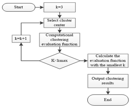
Determine the number of clustering k. By adjusting the evaluation function of smart grid to adjust the number of clusters in the smart grid, the optimal clustering number can be obtained. The definition of evaluation function is given by
Where
where N is the total number of smart grid data, n is the number of samples for each load curve in smart grid,
Data clustering steps in smart grid based on demand response:
First:select kmax.
Second:For k = 3 to kmax.
Third:starting from the last data of the smart grid data set, k smart grid data centers are selected with 2 step size.
Fourth:thedata in smart grid is classified to the nearest class.
Fifth:update the cluster center of smart grid.
Sixth:repeat the Fourth and Fourth. Analyze whether the value of smart grid cluster center changes, and go to the next step.
Seventh:calculate Weight(k).
Eighth:compare Weight(k) and Weight(k−1), save the minimum value k of the evaluation function and continue to iteration.
Ninth: output the best number of clusters of smart grid data and data for each class.
The flow chart of the smart grid data clustering is shown in Figure 2.
Smart grid data clustering
For the ith point of smart grid data, the variation range of load curve in smart grid load is calculated on the basis of calculating the load change rate of the normal load data point in the smart grid. The load data of each smart grid varies within a certain range. In smart grid with different scenarios, the range of load variation is different. Therefore, by increasing or weakening this criterion, we can reduce or magnify the analysis of suspicious data points in smart grid. Since the definition is not necessarily entirely accurate, there will be some errors in judging the suspicious data of smart grid. This error includes misjudgment or omission of smart grid data [1920, 21, 22, 23, 24, 25, 26]. The n daily load curves of the smart grid to be restored are clustered to obtain the k daily load characteristic curves. The normal load point near the data point of the smart grid
The k load characteristic curves are obtained by clustering the load data of smart grid.
Remove the positive and negative load points of the smart grid to be restored from the daily load point curve.
Calculate the distance scale from m points around the load point to be restored to the smart grid load characteristic curve response point.
The nearest load characteristic curve selected from the point scale is used as the reference curve of the corrected data.
According to the characteristics of the load curve of the smart grid, the translation method is used to repair the load curve. The corresponding part of the load characteristic curve X t is translated to the load curve Xc of the smart grid to be detected. It can better reflects the trend of load curve of smart grid, which is expressed as
Where X d is the corrected load curve, is the control coefficient, i = p, p + 1, ..., q. By modifying the load characteristic curve and analyzing the changing trend of the load curve of the smart grid, the input voltage threshold β is input during the operation of the smart grid, and the load optimization control of the smart grid under the different scenarios based on demand response is realized, which is expressed as
3 Results
The experiment uses CPU with memory of 2G, the running system is Windows XP, and the running software is MAT-LAB. In order to verify the effectiveness of the proposed method, the load optimization control algorithm of smart grid under different scenarios based on demand response is used for experiment. Taking the 4 × 300NW unit of a coal power plant as an example, the experimental data of coal consumption rate and power consumption of each unit are shown in Table 1
Experimental data of coal consumption rate of unit power supply
| No. 1 unit | No. 2 unit | No. 3 unit | No. 4 unit | |||||
|---|---|---|---|---|---|---|---|---|
| Load /NW | Coal consumption rate of power supply / [g·(kWh)-1] | Power supply coal consumption /th | Coal consumption rate of power supply / [g·(kWh)-1] | Power supply coal consumption /th | Coal consumption rate of power supply / [g·(kWh)-1] | Power supply coal consumption /th | Coal consumption rate of power supply / [g·(kWh)-1] | Power supply coal consumption /th |
| 200 | 312.50 | 65.66 | 310.12 | 66.33 | 315.31 | 65.25 | 313.24 | 64.38 |
| 210 | 322.88 | 67.23 | 312.23 | 65.11 | 316.58 | 66.11 | 315.19 | 65.16 |
| 220 | 315.66 | 72.15 | 315.02 | 69.36 | 313.22 | 68.16 | 316.23 | 70.22 |
| 235 | 318.36 | 75.25 | 314.69 | 68.24 | 314.84 | 65.28 | 318.15 | 62.33 |
| 255 | 325.12 | 76.88 | 316.32 | 65.34 | 315.22 | 67.32 | 319.22 | 68.54 |
| 265 | 316.33 | 78.26 | 318.75 | 76.45 | 319.52 | 75.15 | 317.15 | 77.49 |
| 270 | 318.22 | 80.05 | 312.01 | 78.92 | 314.11 | 79.16 | 314.32 | 79.39 |
| 275 | 311.89 | 90.66 | 319.36 | 88.52 | 317.56 | 89.92 | 312.05 | 89.62 |
| 280 | 315.65 | 95.12 | 317.22 | 89.37 | 317.26 | 90.36 | 311.09 | 90.38 |
| 300 | 314.06 | 98.55 | 315.41 | 92.12 | 315.14 | 95.88 | 314.44 | 95.13 |
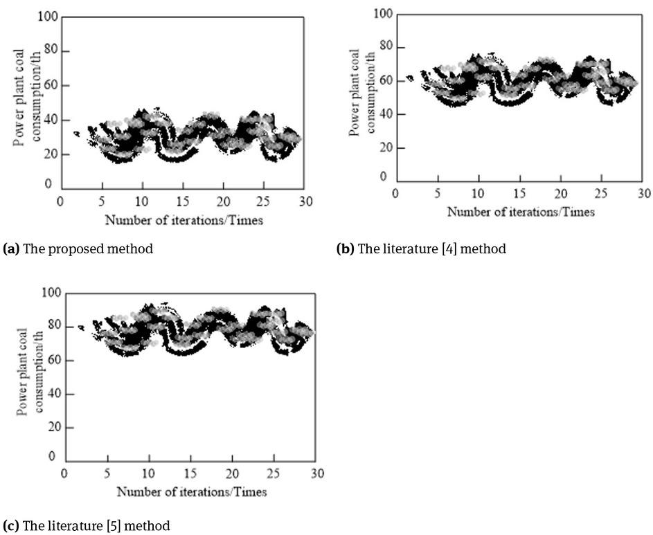
Under different load conditions, there is not much difference between the coal consumption rate per unit and the power consumption of coal consumption per unit. Combined with Table 1, the coal consumption of coal power plant is tested by load control of smart grid. Experimental comparison is shown in Figure 3.
Comparison of coal consumption control
From Figure 3, it can be seen that, for the proposed method, with the change of iteration times, the power consumption of coal and power plants can be controlled
to 20th~50th by using smart grid load. The literature [4] method can control coal consumption of coal and power plants to 40th~80th. The literature [5] method can control coal consumption of coal and power plants to 60th~100th. The proposed method can control the coal consumption of the coal power plant at the lowest level, indicating that the economic effect of the proposed method is better, and the safety and stability of the operation of the whole plant of the coal power plant is improved. Onthis basis, 5 load sampling points (a, b, c, d, and e) in the smart grid are used to test the control coefficient of the load of smart grid under different scenes. The more close to 1 of the control coefficient, the stronger the control performance. The unit of control coefficient is u. The comparison results are shown in Figure 4.

Performance comparison of load optimization control in smart grid
From Figure 4, it can be seen that, among the three methods, when the smart grid is in operation, it is easy to generate a large number of loads, so it is necessary to optimize the control of the loads generated by the smart grid. The load control coefficient obtained with the proposed method is between 0.6~1. The load control coefficient obtained with the literature [5] method is between 0.4~0.8. The load control coefficient obtained with the literature [6] method is between 0.2~0.6. The load control coefficient of the proposed method is close to 1, which indicates that the proposed method has better control performance and can better control the load produced during the operation of the smart grid. On the basis of the above two experiments, 10 groups of smart grid operation data are designed, which are 100, 200, 300, 400, 500, 600, 700, 800, 900, 1000 respectively. The efficiency of smart grid under different scenarios is tested. The results are shown in Table 2.
Comparison of smart grid operating efficiency under different scenarios
| Operating efficiency /% | |||
|---|---|---|---|
| Running data | The proposed method | The literature [4] method | The literature [6] method |
| 100 | 99 | 80 | 69 |
| 200 | 98 | 80 | 69 |
| 300 | 98 | 79 | 68 |
| 400 | 96 | 79 | 67 |
| 500 | 96 | 79 | 67 |
| 600 | 96 | 78 | 66 |
| 700 | 95 | 76 | 66 |
| 800 | 95 | 76 | 66 |
| 900 | 95 | 75 | 65 |
| 1000 | 95 | 72 | 60 |
From Table 2, it can be seen that, in the proposed method, when the running data of smart grid is 100, the corresponding operating efficiency is 99%. When the running data of smart grid is 200 and 300, the operating efficiency is 98%. When the data is running between 400~600, the corresponding operating efficiency is 96%. When the running data are 700, 800, 900 and 1000, the corresponding data operating efficiency is 95%. With the increase of data in smart grid, the operating efficiency is slowly reduced, and the overall operating efficiency is between 95%~99%. In the literature [4] method, the operating efficiency of the 10 sets of smart grid corresponds to 72%~80%. In the literature [6] method, the operating efficiency of the 10 sets of smart grid corresponds to 60%~69%. The comparison results show that the proposed method can effectively control the load of smart grid.
4 Discussions
Through the analysis of the optimal control results of the smart grid load in different scenes, the impact of the threshold of the smart grid voltage β on the precision of the smart grid load control is discussed. When the voltage threshold of smart grid is between 1~2, the precision of smart grid load control is the highest. The unit of voltage threshold is δ. The discussion results are shown in Figure 5
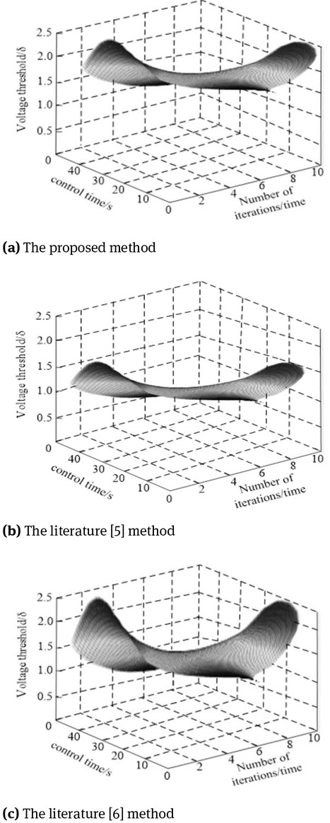
Precision control of smart grid load
From Figure 5, it can be seen that, the voltage threshold of the proposed method is controlled between 0.8~2.1. The voltage threshold of the literature [6] method is controlled below 1.5. In the literature [7] method, the voltage threshold of smart grid is controlled in a wide range, between 0~2.5. From the comparison results, it can be seen that the voltage threshold of the proposed method is close to the 1~2, which proves that the proposed method has high precision in the smart grid load control, and can accurately control the load in the smart grid.
5 Conclusions
In this paper, based on demand response method, load optimization control of smart grid under different scenarios is studied in depth. Taking the experimental data of coal consumption rate and coal consumption in coal-fired power plant as an example, the control of coal consumption is analyzed, and good results are obtained.
The study is divided into three stages to analyze the load optimization control of smart grid under different scenarios.
Using the load sampling point in the smart grid, the control coefficient of the smart grid load under different scenes is tested. The results show that the proposed method has better control performance.
The efficiency of smart grid data in different scenarios is analyzed to achieve efficient control of smart grid load.
The impact of the threshold of the smart grid voltage on the precision of the smart grid load control is discussed. The results show that the proposed method has high control precision.
References
[1] Cheng R.F., Liu Y., Gao J.C., Optimal Power Supply Control of Load Balance Reconfiguration in Distribution Network, Comput. Simul., 2016, 33(10), 314-319.Search in Google Scholar
[2] Liu K., Cheng Y.F., Li W.P., Power Utilization Control of the Intelligence Community Based on Quantum-Based PSO and Binary PSO, Bulletin Sci. Technol., 2016, 32(3), 140-144.Search in Google Scholar
[3] Yang H.C., Cheng, R.F., He Z.H., Multi-Agent Genetic Algorithm for Optimal Configuration of Distributed Power Supply, Computer Measurement & Control, 2017, 25(11), 201-204.Search in Google Scholar
[4] Chen H., Pan X.Y., Zhang J. A Cluster Evolutionary Algorithm for Power System Economic Load Dispatch Optimization, J. Comp. Res. Develop., 2016, 53(7), 1561-1575.Search in Google Scholar
[5] Jin H.J., Analysis of Chaotic Particle Swarm Optimization Algorithm of Optimal Load Distribution in Thermal Power Plant, Electr. Dev., 2017, 40(1), 212-216.Search in Google Scholar
[6] Wei Q., Yang M., Short Term Load Forecasting Based on Improved Neural Network Algorithm, J. Harbin Univ. of Sci. Technol., 2017, 22(4), 65-69.Search in Google Scholar
[7] Sun Y., Ye H., Li B., An Optimal Control Method for Air Conditioning Load by Considering Comfort and Electricity Expense of Consumers, Modern Electric Power, 2016, 33(5), 30-36.Search in Google Scholar
[8] He K.R., Teng H., Guo N., Optimal Operation of User Side Load Considering Peak-valley Difference, Sci. Technol. Eng., 2016, 16(27), 177-182.Search in Google Scholar
[9] Shen T.T., Lv G.Q., Duan H.J., Research on operation control strategy in two layers for micro-grid based on load peak and valley, Electr. Design Eng., 2017, 25(13), 182-186.Search in Google Scholar
[10] Zeng F.Y., Huang Z.R., Research on short-term grid load forecasting method, Automat. Instrument., 2016, (8), 84-86.Search in Google Scholar
[11] Cao S.H., Lu Q.H., Zhang H.X., SDN Based on Dynamic Traffic Scheduling Method of Server Cluster, J. China Acad. Electr. Inform. Technol., 2016, 11(6), 625-628.Search in Google Scholar
[12] Duan S., Shah-Mansouri V., Wang Z., D-ACB: Adaptive Congestion Control Algorithm for Bursty M2M Traffic in LTE Networks, IEEE Trans. Vehic. Technol., 2016, 65(12), 9847-9861.10.1109/TVT.2016.2527601Search in Google Scholar
[13] Fadlullah Z.M., Takaishi D., Nishiyama H., A dynamic trajectory control algorithm for improving the communication throughput and delay in UAV-aided networks, IEEE Network, 2016, 30(1), 100-105.10.1109/MNET.2016.7389838Search in Google Scholar
[14] Singh B., Shah P., Hussain, I. ISOGI-Q Based Control Algorithm for a Single Stage Grid Tied SPV System, IEEE Trans. Industry Appl., 2018, 54(2), 1136-1145.10.1109/TIA.2017.2784374Search in Google Scholar
[15] Shah P., Hussain I., Singh B., Multi-resonant FLL-based control algorithm for grid interfaced multi-functional solar energy conversion system, LET Sci. Meas. Technol., 2018, 12(1), 49-62.10.1049/iet-smt.2017.0096Search in Google Scholar
[16] Mortaji H., Ow S.H., Moghavvemi M., Load Shedding and Smart-Direct Load Control Using Internet of Things in Smart Grid Demand Response Management, IEEE Trans. Industry Appl., 2017, (99), 1-1.10.1109/IAS.2016.7731836Search in Google Scholar
[17] Nguyen C.L., Lee H.H., Effective power dispatch capability decision method for a wind-battery hybrid power system, LET Gen. Trans. Distrib., 2016, 10(3), 661-668.10.1049/iet-gtd.2015.0078Search in Google Scholar
[18] Konstantelos I., Giannelos S., Strbac G., Strategic Valuation of Smart Grid Technology Options in Distribution Networks, IEEE Trans. Power Syst., 2017, 32(2), 1293-1303.10.1109/PESGM.2017.8274536Search in Google Scholar
[19] Madueño G.C., Nielsen J.J., Dong M.K., Assessment of LTE Wireless Access for Monitoring of Energy Distribution in the Smart Grid, IEEE J. Select. Areas Comm., 2016, 34(3), 675-688.10.1109/JSAC.2016.2525639Search in Google Scholar
[20] Zhang Z., Fang H., Gao F., Multiple-Vector Model Predictive Power Control for Grid-TiedWind Turbine System With Enhanced Steady-State Control Performance, IEEE Trans. Industr. Electr., 2017, 64(8), 6287-6298.10.1109/TIE.2017.2682000Search in Google Scholar
[21] Ramane H.S., Jummannaver R.B., Note on Forgotten Topological Index of Chemical Structure in Drugs, Appl. Math. Nonlin. Sci., 2016, 1(2), 369-374.10.21042/AMNS.2016.2.00032Search in Google Scholar
[22] Guerrini G., Landi E., Peiffer K., Fortunato A., Dry Grinding of Gears for Sustainable Automotive Transmission Production, J. Clean. Prod., 2018, 176, 76-88.10.1016/j.jclepro.2017.12.127Search in Google Scholar
[23] Gao W., Wang Y., Wang W., Shi L., The First Multiplication Atom-Bond Connectivity Index of Molecular Structures in Drugs, Saudi Pharm. J., 2017, 25(4), 548-555.10.1016/j.jsps.2017.04.021Search in Google Scholar PubMed PubMed Central
[24] Liu Z., Teaching Reform of Business Statistics in College and University, Eurasia J. Math. Sci. Technol. Edu., 2017, 13(10), 6901-6907.10.12973/ejmste/78537Search in Google Scholar
[25] Zead I., Saad M., Sanad M.R., Behary M.M., Gadallah K., Shokry A., Photometric and Spectroscopic Studies of the Intermediate - Polar Cataclysmic System Dq Her, Appl.Math. Nonlin. Sci., 2017, 2(1), 181-194.10.21042/AMNS.2017.1.00015Search in Google Scholar
[26] Fuentes Rivas R.M., Santacruz De Leon G., Ramos Leal J.A., Moran Ramirez J., Martin Romero F., Characterization of Dissolved Organic Matter in an Agricultural Wastewater-Irrigated Soil, in Semi Arid Mexico, Rev. Int. Contamin. Ambient., 2017, 33(4), 575-590.10.20937/RICA.2017.33.04.03Search in Google Scholar
© 2018 Chengliang Wang et al., published by De Gruyter
This work is licensed under the Creative Commons Attribution-NonCommercial-NoDerivatives 4.0 License.