[go: up one dir, main page]

Next Issue
Volume 8, July
Previous Issue
Volume 8, May
 
 
applsci-logo

Journal Browser

Journal Browser

Appl. Sci., Volume 8, Issue 6 (June 2018) – 169 articles

Cover Story (view full-size image): 
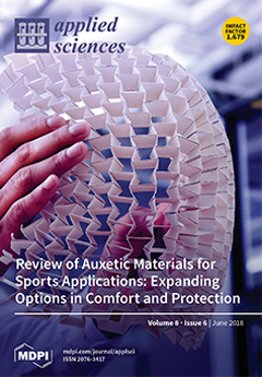
Auxetics expand laterally when stretched, contract when compressed and dome when curved – which should give sports garments unique fit and comfort. Auxetics also provide enhanced hardness and energy absorption, and may reduce rotational acceleration in protective head gear. They open the way for improved protective equipment to reduce injury risk, including concussion and traumatic brain injury, during sporting falls and collisions. The prevalence of sporting injuries and a trend towards form fitting, tailorable garments means manufacturers are looking to auxetics for solutions, and recent developments in Additive Manufacturing and foam and textile production have led to commercial auxetic sports products. View this paper.
  • Issues are regarded as officially published after their release is announced to the table of contents alert mailing list.
  • You may sign up for e-mail alerts to receive table of contents of newly released issues.
  • PDF is the official format for papers published in both, html and pdf forms. To view the papers in pdf format, click on the "PDF Full-text" link, and use the free Adobe Reader to open them.
Order results
Result details
Section
Select all
Export citation of selected articles as:
20 pages, 7315 KiB  
Article
The Effects of Camelina “Soheil” as a Novel Biodiesel Fuel on the Performance and Emission Characteristics of Diesel Engine
by Seyed Salar Hoseini, Gholamhassam Najafi, Barat Ghobadian, Talal Yusaf and Mohammad Taghi Ebadi
Appl. Sci. 2018, 8(6), 1010; https://doi.org/10.3390/app8061010 - 20 Jun 2018
Cited by 14 | Viewed by 5185
Abstract
In this research, a new cultivar of Camelina “Soheil” seed oil (CSO) was investigated as a novel feedstock for biodiesel production. Maximum oil content of CSO seed was about 29%. Physical and chemical characteristics of CSO were investigated. The biodiesel production process was [...] Read more.
In this research, a new cultivar of Camelina “Soheil” seed oil (CSO) was investigated as a novel feedstock for biodiesel production. Maximum oil content of CSO seed was about 29%. Physical and chemical characteristics of CSO were investigated. The biodiesel production process was optimized by using the response surface methodology (RSM) reaction parameters, including molar ratio (methanol to oil), reaction time, and concentration of catalyst are studied. The result showed that the conversion of biodiesel was 98.91% under the optimized conditions of 10.18:1 molar ratio and 1.15 wt % concentration of catalyst for a reaction time of 7.33 min. By investigating the properties of the fuel, it turned out that biodiesel from new cultivar of CSO oil complied with the limits prescribed in the ASTM D6751 standards, and that this seed oil could be introduced as a new feedstock for biodiesel production. Also, the performance and emission of a diesel engine were investigated with CSO biodiesel. All of the engine experiments were performed under the constant speed of 2100 rpm at loads of 0%, 25%, 50%, 75%, and 100%. Results indicated that by using the biodiesel-diesel blends, the brake power, and the CO2 and NOx emissions increased, while the SFC and CO and UHC emissions decreased. Full article
(This article belongs to the Special Issue Renewable Fuels)
Show Figures

Figure 1

Figure 1
<p>Ultrasonic-assisted biodiesel production process: (<b>a</b>) schematic, (<b>b</b>) apparatus.</p>
Full article ">Figure 2
<p>Engine test set-up and test instruments.</p>
Full article ">Figure 3
<p>Effect of molar ratio (methanol to oil)—reaction time on biodiesel yield (%) when catalyst concentration (wt %) is equal to 1.5.</p>
Full article ">Figure 4
<p>Catalyst concentration (wt %)—reaction time (min) on biodiesel conversion (%) when methanol to oil molar ratio equal to 8.11.</p>
Full article ">Figure 5
<p>Results of brake power for different fuel blends at a constant speed of 2100 rpm.</p>
Full article ">Figure 6
<p>Results of specific fuel consumption (SFC) for different fuel blends at the constant speed of 2100 rpm.</p>
Full article ">Figure 7
<p>Results of carbon monoxide (CO) for different fuel blends at the constant speed of 2100 rpm.</p>
Full article ">Figure 8
<p>Results of carbon dioxide (CO<sub>2</sub>) for different fuel blends at the constant speed of 2100 rpm.</p>
Full article ">Figure 9
<p>Results of unburned hydrocarbons (UHC) for different fuel blends at the constant speed of 2100 rpm.</p>
Full article ">Figure 10
<p>Results of nitrogen oxides (NOx) for different fuel blends at the constant speed of 2100 rpm.</p>
Full article ">Figure 11
<p>Impact of the Camelina “Soheil” biodiesel on various engine parameters.</p>
Full article ">
17 pages, 2943 KiB  
Article
Laboratory Evaluation on Performance of Compound-Modified Asphalt for Rock Asphalt/Styrene–Butadiene Rubber (SBR) and Rock Asphalt/Nano-CaCO3
by Songtao Lv, Shuangshuang Wang, Tong Guo, Chengdong Xia, Jianglong Li and Gui Hou
Appl. Sci. 2018, 8(6), 1009; https://doi.org/10.3390/app8061009 - 20 Jun 2018
Cited by 32 | Viewed by 4869
Abstract
As a natural modifier of asphalt, rock asphalt has been widely used to improve its thermal stability and aging resistance. However, the thermal cracking resistance of asphalt modified by rock asphalt is unsatisfactory. In order to improve the thermal cracking resistance in low [...] Read more.
As a natural modifier of asphalt, rock asphalt has been widely used to improve its thermal stability and aging resistance. However, the thermal cracking resistance of asphalt modified by rock asphalt is unsatisfactory. In order to improve the thermal cracking resistance in low temperature, two kinds of modifiers—styrene–butadiene rubber (SBR) and nano-CaCO3—were selected as the compound modifiers, and then implemented to improve the low-temperature performance of the binder. Then, compound asphalt modified by Buton rock asphalt (BRA) was chosen as the study subject. The thermal stability and aging resistance of asphalt modified by BRA, compound-modified asphalt by BRA/SBR, and compound-modified asphalt by BRA and nano-CaCO3 were determined to identify whether the compound modifiers in the asphalt would have a negative effect on the thermal stability and aging resistance of the asphalt. The dynamic shear rheometer (DSR) test was employed to evaluate the thermal stability. The thin film oven test (TFOT) and pressure aging vessel (PAV) were adopted to determine the aging resistance. The viscoelastic characteristics of asphalt with and without modifiers were revealed to evaluate the low-temperature crack resistance of asphalt modified by compound modifiers. The bending beam rheometer (BBR) creep test was conducted in three test temperatures in order to determine the creep stiffness modulus of the BRA compound-modified asphalt. The viscoelastic model considering the damage caused by loading was established; then, the creep compliance and parameters of the viscoelastic damage model were implemented to evaluate the low-temperature performance of the compound-modified asphalt. The results show that the compound modifiers have little negative effects on the thermal stability and aging resistance of asphalt. The thermal crack resistance of the compound-modified asphalt by BRA/SBR was the best, followed by the compound-modified asphalt by BRA and nano-CaCO3 within the three materials. The accuracy of forecasting the characteristics of compound-modified asphalt was improved by using the viscoelastic model and considering the damage effect. Full article
Show Figures

Graphical abstract

Graphical abstract
Full article ">Figure 1
<p>Materials: (<b>a</b>) Buton rock asphalt (BRA); (<b>b</b>) styrene–butadiene rubber (SBR); (<b>c</b>) Nano-CaCO<sub>3</sub>.</p>
Full article ">Figure 2
<p>The relationship between complex shear modulus <span class="html-italic">G*</span> and the temperature of nano-CaCO<sub>3</sub>/BRA and SBR/BRA compound-modified asphalt.</p>
Full article ">Figure 3
<p>The relationship between phase angle <span class="html-italic">δ</span> and temperature of nano-CaCO<sub>3</sub>/BRA and SBR/BRA compound-modified asphalt.</p>
Full article ">Figure 4
<p>The relationship between anti-rutting factors <span class="html-italic">G*</span>/sin<span class="html-italic">δ</span> and the temperature of nano-CaCO<sub>3</sub>/BRA and SBR/BRA compound-modified asphalt.</p>
Full article ">Figure 5
<p>The relationship between Nano-CaCO<sub>3</sub>/BRA and SBR/BRA compound-modified asphalt in before and after thin film oven test (TFOT) aging anti-rutting factors (<span class="html-italic">G*</span>/sin<span class="html-italic">δ</span>) and temperature.</p>
Full article ">Figure 6
<p>Creep stiffness <span class="html-italic">S</span> of nano-CaCO<sub>3</sub>/BRA and SBR/BRA compound-modified asphalt before and after pressure aging vessel (PAV) aging.</p>
Full article ">Figure 7
<p><span class="html-italic">m</span> value of nano-CaCO<sub>3</sub>/BRA and SBR/BRA compound-modified asphalt before and after pressure aging vessel (PAV) aging.</p>
Full article ">Figure 8
<p>Thermoelectric bending beam rheometer (BBR) and specimen: (<b>a</b>) metal die of BBR; (<b>b</b>) asphalt beam of BBR; (<b>c</b>) thermoelectric bending beam rheometer.</p>
Full article ">Figure 9
<p>Creep compliance curve of different compound-modified asphalts: (<b>a</b>) the curves of creep compliance of BRA compound-modified asphalt in −6 °C; (<b>b</b>) the curves of creep compliance of BRA compound-modified asphalt in −12 °C; (<b>c</b>) the curves of creep compliance of BRA compound-modified asphalt in −18°C.</p>
Full article ">Figure 10
<p>Burgers’ model.</p>
Full article ">Figure 11
<p>The comparison among viscoelastic damage model’s parameters of creep compliance: (<b>a</b>) the viscoelastic parameters (<span class="html-italic">E</span><sub>1</sub>) of the model changed with temperature; (<b>b</b>) the viscoelastic parameters (<span class="html-italic">E</span><sub>2</sub>) of the model changed with temperature; (<b>c</b>) the viscoelastic parameters (<span class="html-italic">η</span><sub>1</sub>) of the model changed with temperature; (<b>d</b>) the viscoelastic parameters (<span class="html-italic">η</span><sub>2</sub>) of the model changed with temperature.</p>
Full article ">
17 pages, 3806 KiB  
Article
Modelling Shear Induced Diffusion Based Particle Segregation: A Basis for Novel Separation Technology
by Ivon Drijer and Karin Schroën
Appl. Sci. 2018, 8(6), 1008; https://doi.org/10.3390/app8061008 - 20 Jun 2018
Cited by 8 | Viewed by 5028
Abstract
Shear induced diffusion (SID) based flow segregation is a technique that can be used for concentration and fractionation purposes, and it has the potential to become an economical and sustainable alternative for e.g., membrane separation. When compared to conventional microfiltration, problems related to [...] Read more.
Shear induced diffusion (SID) based flow segregation is a technique that can be used for concentration and fractionation purposes, and it has the potential to become an economical and sustainable alternative for e.g., membrane separation. When compared to conventional microfiltration, problems related to fouling and cleaning are expected to be minimal. To make the best use of the opportunities that this technique holds, detailed insights in flow and particle behavior are needed. Modelling this process allows for us to chart particle segregation in flow, as well as the effect of suspension removal through a pore and the restoration of the flow profile after the pore. As a starting point, we take the computation fluid dynamics (CFD) model that is presented in a previous study. A difference in channel height to particle diameter ratio influences the entrance length of the SID profile as well as its fully developed profile. When extracting liquid through one pore, particles are systematically transmitted at a lower concentration (59–78%) than is present in the bulk. The recovery lengths of the SID profile after the pore were short, and thus pores can be placed at realistic distances, which forms a good foundation for further design of this novel separation technology that will ultimately be applied for fractionation of particles taking relatively small differences in diffusive behavior as a starting point. Full article
Show Figures

Figure 1

Figure 1
<p>Flux versus the particle diameter for different migration mechanisms (Graph is reprinted from Separation and Purification Technology, 174, Karin Schroën; Anna van Dinther and Regine Stockmann, Particle migration in laminar shear fields: A new basis for large scale separation technology?, 372–388, 2017, with permission from Elsevier, original is from Davis [<a href="#B11-applsci-08-01008" class="html-bibr">11</a>]).</p>
Full article ">Figure 2
<p>Schematic representation of the segregation principle of shear induced diffusion for a bidisperse (<b>a</b>) and monodisperse (<b>b</b>) suspension.</p>
Full article ">Figure 3
<p>Schematic view of the process considered in this study; please note the change in concentration profile close to the pore that will be discussed in detail in the results section.</p>
Full article ">Figure 4
<p>Flow chart of the most important steps taken in our shear induced diffusion model.</p>
Full article ">Figure 5
<p>(<b>a</b>) Particle volume fraction versus the channel height and (<b>b</b>) the particle volume fraction in the center of the channel versus the channel length for different friction factors for both the drag and Shear induced diffusion (SID) force: <math display="inline"> <semantics> <mrow> <mi>f</mi> <mrow> <mo>(</mo> <mrow> <msub> <mi>α</mi> <mi>p</mi> </msub> </mrow> <mo>)</mo> </mrow> </mrow> </semantics> </math> for SID and <math display="inline"> <semantics> <mrow> <msubsup> <mi>f</mi> <mrow> <mi>i</mi> <mi>j</mi> </mrow> <mi>D</mi> </msubsup> </mrow> </semantics> </math> for drag (black solid line); <math display="inline"> <semantics> <mrow> <mi>f</mi> <mrow> <mo>(</mo> <mrow> <msub> <mi>α</mi> <mi>p</mi> </msub> </mrow> <mo>)</mo> </mrow> </mrow> </semantics> </math> for both SID and drag (grey solid line); <math display="inline"> <semantics> <mrow> <msubsup> <mi>f</mi> <mrow> <mi>i</mi> <mi>j</mi> </mrow> <mi>D</mi> </msubsup> </mrow> </semantics> </math> for both SID and drag (black dashed line); and, <math display="inline"> <semantics> <mrow> <msubsup> <mi>f</mi> <mrow> <mi>i</mi> <mi>j</mi> </mrow> <mi>D</mi> </msubsup> <mtext> </mtext> </mrow> </semantics> </math> for SID and <math display="inline"> <semantics> <mrow> <mi>f</mi> <mrow> <mo>(</mo> <mrow> <msub> <mi>α</mi> <mi>p</mi> </msub> </mrow> <mo>)</mo> </mrow> </mrow> </semantics> </math> for drag (grey dashed line)</p>
Full article ">Figure 6
<p>(<b>a</b>) Particle volume fraction versus the channel length at the channel centerline and (<b>b</b>) at 10% from the wall. Results are shown for a bulk particle volume fraction of 30% and for the cases as given in <a href="#applsci-08-01008-t004" class="html-table">Table 4</a>: case 1 (solid line); case 2 (dashed line); case 3 (dashed-dotted line); and, case 4 (dotted line). Note that case 1 and 4 overlap.</p>
Full article ">Figure 7
<p>(<b>a</b>) Particle volume fraction versus the channel length at the channel centerline and (<b>b</b>) at 10% from the wall. Results are shown for three different bulk particle volume fractions: 0.1 (light grey); 0.3 (dark grey); 0.5 (black) and for the cases as given in <a href="#applsci-08-01008-t004" class="html-table">Table 4</a>: case 1 (solid line); case 2 (dashed line); case 3 (dashed-dotted line); and, case 4 (dotted line). Note, case 1 and 4 overlap.</p>
Full article ">Figure 8
<p>Increase in particle volume fraction at the center versus the bulk particle volume fraction for fully developed profiles for case 4 given in <a href="#applsci-08-01008-t004" class="html-table">Table 4</a>.</p>
Full article ">Figure 9
<p>Transmission versus the volume fraction taken form the inlet. Results are shown for a channel height of 50 (circles) and 100 (squares) µm and for three different bulk particle volume fractions: 0.1 (dark grey); 0.3 (light grey); and, 0.5 (black).</p>
Full article ">Figure 10
<p>Particle volume fraction versus the relative channel height. The graph gives an indication of the shift in the SID profile of a suspension with a 50% bulk particle volume fraction: fully developed SID profile before the pore at 9.5 cm (black line, 1); disturbed SID profile just after the pore at ~10 cm (light grey line, 2) and the restored SID profile after the pore at 19.5 cm (dark grey line, 3).</p>
Full article ">Figure 11
<p>Relative development length at the center of the channel (95%) between the recover section and the entrance section versus the volume fraction extracted from the inlet for a bulk particle volume fraction of 10% (<b>a</b>) and 30% (<b>b</b>). Each graph shows two different lines for the different channel heights: 50 µm (black) and 100 µm (grey).</p>
Full article ">Figure 12
<p>Relative particle volume fraction versus the relative channel height at a fully developed profile before the porous region for two different bulk particle volume fractions: 10% (black) and 30% (grey) and two different channel heights: 50 µm (solid line) and 100 µm (dashed line). Vertical lines indicate the amount of volume extracted, from left to right: 2.5%, 5%, 7.5%, and 10%.</p>
Full article ">Figure A1
<p>Grid refinement study for case 1. The relative particle volume fraction versus the channel height, measured 2.5 cm from the channel entrance. The grid cell number of the channel height is changed: 7 grid cells (black solid line); 11 grid cells (grey solid line); 15 grid cells (black dashed line); 19 grid cells (grey dashed line) and 23 grid cells (black dashed-dotted line) (Graph is reprinted from Separation and Purification Technology, 192, I. Drijer; T. van de Laar; H.M. Vollebregt and C.G.P.H. Schroën, From highly specialised to generally available modelling of shear induced particle migration for flow segregation based separation technology, 99–109, 2018, with permission from Elsevier).</p>
Full article ">Figure A2
<p>Grid refinement study for case 2. The relative particle volume fraction versus the channel height, measured 2.5 cm from the channel entrance. The grid cell number of the channel height is changed: 37 grid cells (black solid line); 41 grid cells (grey solid line); 45 grid cells (black dashed line); 47 grid cells (grey dashed line) and 49 grid cells (black dashed-dotted line).</p>
Full article ">Figure A3
<p>Grid refinement study for case 3. The relative particle volume fraction versus the channel height, measured 2.5 cm from the channel entrance. The grid cell number of the channel height is changed: 15 grid cells (black solid line); 19 grid cells (grey solid line); 21 grid cells (black dashed line); 23 grid cells (grey dashed line) and 27 grid cells (black dashed-dotted line).</p>
Full article ">Figure A4
<p>Grid refinement study for case 4: the length and height of the pore. The relative particle volume fraction versus the channel height, measured at the center of the pore in the vertical (<b>a</b>) and horizontal (<b>b</b>) direction. The grid cell number for both the height (h) and the length (l) is changed: h = 5 and l = 9 (black solid line); h = 7 and l = 9 (grey solid line); h = 9 and l = 9 (black dashed line); h = 11 and l = 9 (grey dashed line); h = 9 and l = 5 (black dashed-dotted line), h = 9 and l = 7 (grey dashed-dotted line) and h = 9 and l = 7 (black dashed-double dotted line).</p>
Full article ">Figure A5
<p>Schematic overview of how the entrance length is determined at the center of the channel and at 95% of the fully developed value. SID profile (black solid line); relative particle volume fraction for a fully developed profile (horizontal black dotted line); relative particle volume fraction at 95% (grey horizontal dotted line); tangent at 95% of the fully developed profile (grey solid line).</p>
Full article ">
16 pages, 3009 KiB  
Article
Modified LMS Strategies Using Internal Model Control for Active Noise and Vibration Control Systems
by Byeongil Kim and Jong-Yun Yoon
Appl. Sci. 2018, 8(6), 1007; https://doi.org/10.3390/app8061007 - 20 Jun 2018
Cited by 8 | Viewed by 4744
Abstract
Traditional adaptive filtering algorithms are non-recursive systems that cannot use a time-variant reference input in real time and are not appropriate for control signals with uncertainties and unanticipated conditions. The main purpose of this research is to design novel adaptive digital filtering algorithms [...] Read more.
Traditional adaptive filtering algorithms are non-recursive systems that cannot use a time-variant reference input in real time and are not appropriate for control signals with uncertainties and unanticipated conditions. The main purpose of this research is to design novel adaptive digital filtering algorithms based on internal model control (IMC). The new methods consist of a process model for the target plant so as to estimate its dynamic behavior for active vibration and noise attenuation schemes in order to improve the stability, robustness, and tracking performance. On the basis of on the existing least mean squares, the methods are combined with an internal model controller, or the whole adaptive filtering system could become a feedback control system structure based on IMC. The performances were validated in numerical simulations with various conditions that could have happened in realistic applications, and the results were compared with the original algorithms. This study shows that the active noise and vibration systems that are applied to vehicles, mechanical systems, and other targets are enhanced through improving the performance of conventional adaptive filtering algorithms and by using internal model control effectively. Full article
(This article belongs to the Special Issue Active and Passive Noise Control)
Show Figures

Figure 1

Figure 1
<p>Digital filtering system with filtered-X least mean square (FX-LMS) algorithm.</p>
Full article ">Figure 2
<p>Internal model control (IMC) system.</p>
Full article ">Figure 3
<p>Schematic of a new digital filtering system with LMS, based on the internal model control (IM-LMS 1).</p>
Full article ">Figure 4
<p>Simulation results in time domain with a single sinusoid at 100 Hz. (<b>a</b>) Time domain tracking with LMS and internal model LMS 1 methods; (<b>b</b>) estimation error; (<b>c</b>) predicted spectra.</p>
Full article ">Figure 4 Cont.
<p>Simulation results in time domain with a single sinusoid at 100 Hz. (<b>a</b>) Time domain tracking with LMS and internal model LMS 1 methods; (<b>b</b>) estimation error; (<b>c</b>) predicted spectra.</p>
Full article ">Figure 5
<p>Simulation results in the time domain (single sinusoid at 100 Hz) with LMS and internal model LMS 1 methods. (<b>a</b>) With exact model (top) and with uncertainty (bottom); (<b>b</b>) comparison of estimation error; (<b>c</b>) predicted spectra.</p>
Full article ">Figure 5 Cont.
<p>Simulation results in the time domain (single sinusoid at 100 Hz) with LMS and internal model LMS 1 methods. (<b>a</b>) With exact model (top) and with uncertainty (bottom); (<b>b</b>) comparison of estimation error; (<b>c</b>) predicted spectra.</p>
Full article ">Figure 6
<p>Control of an amplitude-modulated (AM) signal. (<b>a</b>) Time-domain tracking with LMS and internal model LMS 1 methods; (<b>b</b>) estimation error; (<b>c</b>) predicted spectra.</p>
Full article ">Figure 7
<p>Schematic of a novel digital filter system with ‘recursive’ LMS algorithm, based on internal model control (IM-LMS 2).</p>
Full article ">Figure 8
<p>Control of an amplitude-modulated (AM) signal. (<b>a</b>) Time-domain tracking with LMS and internal model LMS 2 methods; (<b>b</b>) estimation error.</p>
Full article ">Figure 9
<p>Predicted spectra for an amplitude-modulated (AM) signal with LMS and internal model LMS 2 methods.</p>
Full article ">Figure 10
<p>Control of a frequency-modulated (FM) signal. (<b>a</b>) Time-domain tracking with LMS and internal model LMS 2 methods; (<b>b</b>) estimation error.</p>
Full article ">Figure 11
<p>Predicted spectra for a frequency-modulated (FM) signal with least mean squares and internal model least mean squares 2 methods.</p>
Full article ">
9 pages, 2466 KiB  
Article
Programmable Zoom Lens System with Two Spatial Light Modulators: Limits Imposed by the Spatial Resolution
by Jeffrey A. Davis, Trevor I. Hall, Ignacio Moreno, Jason P. Sorger and Don M. Cottrell
Appl. Sci. 2018, 8(6), 1006; https://doi.org/10.3390/app8061006 - 20 Jun 2018
Cited by 11 | Viewed by 4309
Abstract
In this work we present an experimental proof of concept of a programmable optical zoom lens system with no moving parts that can form images with both positive and negative magnifications. Our system uses two programmable liquid crystal spatial light modulators to form [...] Read more.
In this work we present an experimental proof of concept of a programmable optical zoom lens system with no moving parts that can form images with both positive and negative magnifications. Our system uses two programmable liquid crystal spatial light modulators to form the lenses composing the zoom system. The results included show that images can be formed with both positive and negative magnifications. Experimental results match the theory. We discuss the size limitations of this system caused by the limited spatial resolution and discuss how newer devices would shrink the size of the system. Full article
Show Figures

Figure 1

Figure 1
<p>Schematic of the zoom lens optical system.</p>
Full article ">Figure 2
<p>Phase patterns for diffractive lenses having focal lengths of (<b>a</b>) 3<span class="html-italic">f<sub>N</sub></span>, (<b>b</b>) <span class="html-italic">f<sub>N</sub></span> and (<b>c</b>) <span class="html-italic">f<sub>N</sub></span>/3.</p>
Full article ">Figure 3
<p>Input object captured by camera. Here the slide with the word “PROFESSOR” is placed directly to the detector. The size of the object slightly exceeds the size of the detector.</p>
Full article ">Figure 4
<p>Zoom system configuration with <span class="html-italic">f</span><sub>1</sub> = 70.2 cm and <span class="html-italic">f</span><sub>2</sub> = ∞ and experimental image with magnification of <span class="html-italic">m</span> = −2.4.</p>
Full article ">Figure 5
<p>Zoom system configuration with <span class="html-italic">f</span><sub>1</sub> = ∞ and <span class="html-italic">f</span><sub>2</sub> = +69.6 cm and experimental image with magnification of <span class="html-italic">m</span> = −0.4.</p>
Full article ">Figure 6
<p>Zoom system configuration with <span class="html-italic">f</span><sub>1</sub> = +100 cm and <span class="html-italic">f</span><sub>2</sub> = +100 cm and experimental image with magnification of <span class="html-italic">m</span> = −1.</p>
Full article ">Figure 7
<p>Zoom system configuration with <span class="html-italic">f</span><sub>1</sub> = +50 cm and <span class="html-italic">f</span><sub>2</sub> = +31.8 cm and experimental image with magnification of <span class="html-italic">m</span> = +2.</p>
Full article ">Figure 8
<p>Zoom system configuration with <span class="html-italic">f</span><sub>1</sub> = +31.8 cm and <span class="html-italic">f</span><sub>2</sub> = +50 cm and experimental image with magnification of <span class="html-italic">m</span> = +0.5.</p>
Full article ">Figure 9
<p>Zoom system configuration with <span class="html-italic">f</span><sub>1</sub> = +40 cm and <span class="html-italic">f</span><sub>2</sub> = +44 cm and experimental image with magnification of <span class="html-italic">m</span> = +1.</p>
Full article ">
15 pages, 2970 KiB  
Article
The Use of Co-Precipitation to Produce Nano-Mn–Zn Ferrite ([MnxZn1?x]Fe2O4) from Waste Batteries
by Yenchun Liu and Jarnchih Hsu
Appl. Sci. 2018, 8(6), 1005; https://doi.org/10.3390/app8061005 - 20 Jun 2018
Cited by 11 | Viewed by 4370
Abstract
This study uses pure materials or waste batteries to produce a nanoscale Mn–Zn ferrite. Acid is used to dissolve the battery into solution and then co-precipitation is used to produce nanoscale ferrite. When the calcination temperature in an air atmosphere exceeds 600 °C, [...] Read more.
This study uses pure materials or waste batteries to produce a nanoscale Mn–Zn ferrite. Acid is used to dissolve the battery into solution and then co-precipitation is used to produce nanoscale ferrite. When the calcination temperature in an air atmosphere exceeds 600 °C, α-Fe2O3 is generated and there is a decrease in the saturated magnetization. Using waste batteries to produce [Mn0.54Zn0.46]Fe2O4 at a pH of 10, the saturated magnetization is 62.85 M (emu/g), which is optimal. At a pH of 10, the particulate diameter is largest, at about 40 nm. The stronger the crystal phase of Mn–Zn ferrite, the greater is the saturated magnetization. The ferrite crystal phase is analyzed using X-ray diffraction (XRD), scanning electron microscopy (SEM) and a vibrating sample magnetometer (VSM). The stronger the crystal phase, the larger is the average particulate diameter. The magnetic properties, the particulate diameter and the magnetic flux density of ferrite powders that are prepared under different conditions are studied. [MnxZn1−x]Fe2O4 ferrite powders can be used as an iron core and as resonance imaging materials. Full article
(This article belongs to the Section Materials Science and Engineering)
Show Figures

Figure 1

Figure 1
<p>The synthesis of [Mn<sub>x</sub>Zn<sub>1−x</sub>]Fe<sub>2</sub>O<sub>4</sub> ferrite from waste battery.</p>
Full article ">Figure 2
<p>XRD patterns for (<b>a</b>) [Mn<sub>x</sub>Zn<sub>1−x</sub>]Fe<sub>2</sub>O<sub>4</sub> sintered at 600 °C and (<b>b</b>) the effect of the pH value of the waste dry battery.</p>
Full article ">Figure 3
<p>The hysteresis curves for different compositions and proportions; [M<sub>x</sub>Zn<sub>1−x</sub>]Fe<sub>2</sub>O<sub>4</sub> (M = Mn, Zn, Cu).</p>
Full article ">Figure 4
<p>The effect of the pH value on the magnetic properties of [Mn<sub>0.54</sub>Zn<sub>0.46</sub>]Fe<sub>2</sub>O<sub>4</sub> that is produced from waste dry batteries.</p>
Full article ">Figure 5
<p>The effect of the sintering temperature in an air atmosphere on (<b>a</b>) the crystal phase and (<b>b</b>) the magnetic properties.</p>
Full article ">Figure 6
<p>The surface morphology of [Mn<sub>0.54</sub>Zn<sub>0.46</sub>]Fe<sub>2</sub>O<sub>4</sub> that is produced from waste dry batteries with different pH values: (<b>a</b>) pH = 6, (<b>b</b>) pH = 7, (<b>c</b>) pH = 8, (<b>d</b>) pH = 9, (<b>e</b>) pH = 10, (<b>f</b>) pH = 11 and (<b>g</b>) pH = 12.</p>
Full article ">Figure 6 Cont.
<p>The surface morphology of [Mn<sub>0.54</sub>Zn<sub>0.46</sub>]Fe<sub>2</sub>O<sub>4</sub> that is produced from waste dry batteries with different pH values: (<b>a</b>) pH = 6, (<b>b</b>) pH = 7, (<b>c</b>) pH = 8, (<b>d</b>) pH = 9, (<b>e</b>) pH = 10, (<b>f</b>) pH = 11 and (<b>g</b>) pH = 12.</p>
Full article ">Figure 7
<p>The effect of sintering temperature in a N<sub>2</sub> environment on (<b>a</b>) the crystal phase and (<b>b</b>) the magnetic properties of Mn<sub>0.54</sub>Zn<sub>0.46</sub>Fe<sub>2</sub>O<sub>4.</sub></p>
Full article ">Figure 8
<p>The effect of forming sintering on the Q-value for different systems.</p>
Full article ">Figure 9
<p>The effect of forming sintering on the μ<sub>0</sub> and R values for different systems.</p>
Full article ">
22 pages, 15804 KiB  
Article
Evaluation of the Implicit Gradient-Enhanced Regularization of a Damage-Plasticity Rock Model
by Magdalena Schreter, Matthias Neuner and Günter Hofstetter
Appl. Sci. 2018, 8(6), 1004; https://doi.org/10.3390/app8061004 - 20 Jun 2018
Cited by 23 | Viewed by 4736
Abstract
In the present publication, the performance of an implicit gradient-enhanced damage-plasticity model is evaluated with special focus on the prediction of complex failure modes such as shear failure. Hence, it complements studies on predominant mode I failure frequently found in the literature. To [...] Read more.
In the present publication, the performance of an implicit gradient-enhanced damage-plasticity model is evaluated with special focus on the prediction of complex failure modes such as shear failure. Hence, it complements studies on predominant mode I failure frequently found in the literature. To this end, an implicit gradient-enhanced damage-plasticity rock model is presented and validated by means of 2D and 3D finite element simulations of both laboratory tests on intact rock specimens as well as a large-scale structural benchmark related to failure of rock mass. Thereby, a wide range of loading conditions comprising unconfined and/or confined, tensile and/or compressive stress states is considered. The capability of the gradient-enhanced rock model for representing the mechanical response objectively with respect to the finite element discretization and realistically compared to measurement data is assessed. It is shown that complex failure modes and the respective load–displacement curves are predicted in a mesh-insensitive manner. Full article
(This article belongs to the Special Issue Computational Methods for Fracture)
Show Figures

Figure 1

Figure 1
<p>Schematic illustration of two characteristic failure modes (according to [<a href="#B23-applsci-08-01004" class="html-bibr">23</a>]): tensile failure (opening mode, <b>left</b>) and shear failure (sliding mode, <b>right</b>).</p>
Full article ">Figure 2
<p>Geometry and boundary conditions of the numerical model of the specimen for the wedge splitting test.</p>
Full article ">Figure 3
<p>Splitting force vs. crack mouth opening displacement (CMOD) for the wedge splitting test: experimental results (data taken from [<a href="#B40-applsci-08-01004" class="html-bibr">40</a>]) and numerical results.</p>
Full article ">Figure 4
<p>Deformed specimen at CMOD = 0.3 mm with a displacement scale factor of 100 for the three structured finite element meshes: coarse—3580 elements (<b>left</b>), medium—6940 elements (<b>center</b>), and fine—15430 elements (<b>right</b>).</p>
Full article ">Figure 5
<p>Distribution of the damage variable <math display="inline"><semantics> <mi>ω</mi> </semantics></math> at CMOD = 0.3 mm for the three structured finite element meshes: coarse (<b>left</b>), medium (<b>center</b>), and fine (<b>right</b>).</p>
Full article ">Figure 6
<p>Deformed specimen with a displacement scale factor of 100 (<b>left</b>) and distribution of the damage variable <math display="inline"><semantics> <mi>ω</mi> </semantics></math> (<b>right</b>) for the unstructured mesh (9504 elements) at a CMOD of 0.3 mm.</p>
Full article ">Figure 7
<p>Geometry and boundary conditions of the specimen for the triaxial compression test.</p>
Full article ">Figure 8
<p>Load–displacement curves (axial force versus axial displacement) for triaxial compression tests: experimental and numerical results for different levels of confining pressures <math display="inline"><semantics> <mrow> <msup> <mi>p</mi> <mrow> <mo>(</mo> <mn>0</mn> <mo>)</mo> </mrow> </msup> </mrow> </semantics></math>.</p>
Full article ">Figure 9
<p>(<b>a</b>) Distribution of the vertical displacement <math display="inline"><semantics> <msub> <mi>u</mi> <mi>z</mi> </msub> </semantics></math> (scale factor 5) in the final stage of the triaxial compression test with <math display="inline"><semantics> <mrow> <msup> <mi>p</mi> <mrow> <mo>(</mo> <mn>0</mn> <mo>)</mo> </mrow> </msup> <mo>=</mo> <mn>37.5</mn> <mrow> <mi>MPa</mi> </mrow> </mrow> </semantics></math> for the three finite element meshes: coarse (<b>left</b>), medium (<b>center</b>), and fine (<b>right</b>). (<b>b</b>) Corresponding deformed rock specimen after a triaxial compression test with <math display="inline"><semantics> <mrow> <msup> <mi>p</mi> <mrow> <mo>(</mo> <mn>0</mn> <mo>)</mo> </mrow> </msup> <mo>=</mo> <mn>37.5</mn> <mrow> <mi>MPa</mi> </mrow> </mrow> </semantics></math>, reproduced with permission from M. Bluemel taken from the report [<a href="#B41-applsci-08-01004" class="html-bibr">41</a>].</p>
Full article ">Figure 10
<p>Distribution of the damage variable <math display="inline"><semantics> <mi>ω</mi> </semantics></math> in the final stage of the triaxial compression test with <math display="inline"><semantics> <mrow> <msup> <mi>p</mi> <mrow> <mo>(</mo> <mn>0</mn> <mo>)</mo> </mrow> </msup> <mo>=</mo> <mn>37.5</mn> <mrow> <mi>MPa</mi> </mrow> </mrow> </semantics></math> for the three finite element meshes: coarse (<b>left</b>), medium (<b>center</b>), and fine (<b>right</b>).</p>
Full article ">Figure 11
<p>Triaxial compression tests: distribution of the vertical displacement <math display="inline"><semantics> <msub> <mi>u</mi> <mi>z</mi> </msub> </semantics></math> in the symmetry plane for the four different levels of confining pressure.</p>
Full article ">Figure 12
<p>Computed load–displacement curves for triaxial extension tests for different levels of confining pressure <math display="inline"><semantics> <mrow> <msup> <mi>p</mi> <mrow> <mo>(</mo> <mn>0</mn> <mo>)</mo> </mrow> </msup> </mrow> </semantics></math>.</p>
Full article ">Figure 13
<p>Distribution of the vertical displacement <math display="inline"><semantics> <msub> <mi>u</mi> <mi>z</mi> </msub> </semantics></math> (deformation scale factor 10) at an applied top displacement of 0.1 mm in the triaxial extension test with <math display="inline"><semantics> <mrow> <msup> <mi>p</mi> <mrow> <mo>(</mo> <mn>0</mn> <mo>)</mo> </mrow> </msup> <mo>=</mo> <mn>37.5</mn> <mrow> <mi>MPa</mi> </mrow> </mrow> </semantics></math> for the three finite element meshes: coarse (<b>left</b>), medium (<b>center</b>), and fine (<b>right</b>).</p>
Full article ">Figure 14
<p>2D initial boundary value problem of deep tunnel excavation: full model (<b>left</b>) and the detail center view (<b>right</b>).</p>
Full article ">Figure 15
<p>Distribution of the magnitude of the displacement vector in the vicinity of the tunnel surface at the level of 12 % of the initial internal pressure with a displacement scale factor of 10 for the three finite element meshes with full numerical integration: coarse (<b>left</b>), medium (<b>center</b>), and fine (<b>right</b>).</p>
Full article ">Figure 16
<p>Load–displacement curves: normalized internal pressure versus the mean displacement magnitude at the tunnel surface for the three finite element meshes with full and reduced numerical integration: total view (<b>left</b>), detailed view (<b>right</b>).</p>
Full article ">Figure 17
<p>Distribution of the damage variable <math display="inline"><semantics> <mi>ω</mi> </semantics></math> in the rock mass in the vicinity of the tunnel surface at the level of 12 % of the internal pressure for the three finite element meshes employing full numerical integration: coarse (<b>left</b>), medium (<b>center</b>), and fine (<b>right</b>).</p>
Full article ">
13 pages, 2211 KiB  
Article
Stability of Cu-Precipitates in Al-Cu Alloys
by Torsten E. M. Staab, Paola Folegati, Iris Wolfertz and Martti J. Puska
Appl. Sci. 2018, 8(6), 1003; https://doi.org/10.3390/app8061003 - 20 Jun 2018
Cited by 8 | Viewed by 5547
Abstract
We present first principle calculations on formation and binding energies for Cu and Zn as solute atoms forming small clusters up to nine atoms in Al-Cu and Al-Zn alloys. We employ a density-functional approach implemented using projector-augmented waves and plane wave expansions. We [...] Read more.
We present first principle calculations on formation and binding energies for Cu and Zn as solute atoms forming small clusters up to nine atoms in Al-Cu and Al-Zn alloys. We employ a density-functional approach implemented using projector-augmented waves and plane wave expansions. We find that some structures, in which Cu atoms are closely packed on {100}-planes, turn out to be extraordinary stable. We compare the results with existing numerical or experimental data when possible. We find that Cu atoms precipitating in the form of two-dimensional platelets on {100}-planes in the fcc aluminum are more stable than three-dimensional structures consisting of the same number of Cu-atoms. The preference turns out to be opposite for Zn in Al. Both observations are in agreement with experimental observations. Full article
(This article belongs to the Special Issue Mechanical Behaviour of Aluminium Alloys)
Show Figures

Figure 1

Figure 1
<p>Configuration of Cu-atoms in 2D platelets on the <math display="inline"><semantics> <mrow> <mo>{</mo> <mn>100</mn> <mo>}</mo> </mrow> </semantics></math>-plane in fcc Al. The Cu and Al atoms are shown by red and grey spheres, respectively. The numbering indicates how the Cu-platelets were assumed to grow. The left and right patterns show the sequences 1 and 2 used in the calculations, respectively.</p>
Full article ">Figure 2
<p>Energy gain during Cu-cluster growth for a supercell of 108 atoms in sequences 1 and 2. (<b>left</b>) The energy gain due to the last attached Cu atom, (<b>right</b>) the total energy gain per Cu atom in the growing cluster. Sequences 1 and 2 are explained in <a href="#applsci-08-01003-f001" class="html-fig">Figure 1</a>.</p>
Full article ">Figure 3
<p>Energy gain during Cu-cluster growth. Results corresponding to supercells of 108, 128, and 192 atoms are compared. (<b>left</b>) Energy gain due to the last Cu atom attached, and (<b>right</b>) total energy gain per Cu-atom of a growing cluster. Sequence 1 is explained in <a href="#applsci-08-01003-f001" class="html-fig">Figure 1</a>.</p>
Full article ">Figure 4
<p>Energy gain during Cu-cluster growth. The results corresponding to the supercells of 108, 128, and 192 atoms are compared. (<b>left</b>) Energy gain of the last Cu atom attached, (<b>right</b>) total energy gain per Cu-atom of a growing cluster. Sequence 2 is explained in <a href="#applsci-08-01003-f001" class="html-fig">Figure 1</a>.</p>
Full article ">Figure 5
<p>Relaxation patterns of growing clusters. (<b>left</b>) Two copper atoms (red spheres) on 1NN position, (<b>right</b>) five Cu-atoms arranged as a platelet on the <math display="inline"><semantics> <mrow> <mo>{</mo> <mn>100</mn> <mo>}</mo> </mrow> </semantics></math>-plane. The Al atoms having two or more bonds to Cu-atoms are plotted in dark-grey color. The relaxation of the Al-layer above and below towards the Cu-atoms on the <math display="inline"><semantics> <mrow> <mo>{</mo> <mn>100</mn> <mo>}</mo> </mrow> </semantics></math>-plane clearly increases with the number of agglomerated Cu-aotms.</p>
Full article ">Figure 6
<p>Total energies calculated by using static (atoms fixed) and relaxed configurations of a supercell of 108 atoms.</p>
Full article ">Figure 7
<p>Binding energies of Zn atoms in 2D and 3D Zn clusters. (<b>left</b>) The binding energy for the last attached Zn atom. (<b>right</b>) The binding energy per Zn atom in the cluster.</p>
Full article ">
11 pages, 3396 KiB  
Article
Manufacturing of Non-Stick Molds from Pre-Painted Aluminum Sheets via Single Point Incremental Forming
by Oscar Rodriguez-Alabanda, Miguel A. Narvaez, Guillermo Guerrero-Vaca and Pablo E. Romero
Appl. Sci. 2018, 8(6), 1002; https://doi.org/10.3390/app8061002 - 20 Jun 2018
Cited by 6 | Viewed by 4593
Abstract
The process of single point incremental formation (SPIF) awakens interest in the industry of mold manufacturing for the food industry. By means of SPIF, it is possible to generate short series of molds or mold prototypes at low cost. However, these industries require [...] Read more.
The process of single point incremental formation (SPIF) awakens interest in the industry of mold manufacturing for the food industry. By means of SPIF, it is possible to generate short series of molds or mold prototypes at low cost. However, these industries require such molds to be functional (non-sticky) and to have an adequate geometry accuracy. This study presents a technique that enables direct manufacturing of molds from pre-coated sheets with non-stick resins. It has also studied the influence of two technological variables in the process (feed-rate and pitch) for different geometrical parameters of the mold. Low values of these variables result in a lower overall error in the profile obtained. However, in order to obtain greater detail in particular parameters (angles, depth), it is necessary to use higher values of feed-rate and pitch. Full article
(This article belongs to the Special Issue Mechanical Behaviour of Aluminium Alloys)
Show Figures

Figure 1

Figure 1
<p>Schematic representation of SPIF process.</p>
Full article ">Figure 2
<p>Dimensions of the mold used in the tests (unit: mm).</p>
Full article ">Figure 3
<p>Experiment set-up and manufactured pieces.</p>
Full article ">Figure 4
<p>Geometrical characterization of the part and error respect to theoretical profile.</p>
Full article ">Figure 5
<p>Experimental angle #1 obtained for different pitches and feed-rates.</p>
Full article ">Figure 6
<p>Experimental angle #2 obtained for different pitches and feed-rates.</p>
Full article ">Figure 7
<p>Minimum thickness obtained in the different tests.</p>
Full article ">Figure 8
<p>Height and depth of the molds, for different pitches and feed-rates.</p>
Full article ">Figure 9
<p>Normalized springback, for different pitches and feed-rates.</p>
Full article ">Figure 10
<p>Area between real and theoretical profiles (global error).</p>
Full article ">Figure 11
<p>Format limit diagram for molds (2000 mm/min).</p>
Full article ">
9 pages, 1064 KiB  
Article
Automatic Bowel Motility Evaluation Technique for Noncontact Sound Recordings
by Ryunosuke Sato, Takahiro Emoto, Yuki Gojima and Masatake Akutagawa
Appl. Sci. 2018, 8(6), 999; https://doi.org/10.3390/app8060999 - 19 Jun 2018
Cited by 12 | Viewed by 4589
Abstract
Information on bowel motility can be obtained via magnetic resonance imaging (MRI)s and X-ray imaging. However, these approaches require expensive medical instruments and are unsuitable for frequent monitoring. Bowel sounds (BS) can be conveniently obtained using electronic stethoscopes and have recently been employed [...] Read more.
Information on bowel motility can be obtained via magnetic resonance imaging (MRI)s and X-ray imaging. However, these approaches require expensive medical instruments and are unsuitable for frequent monitoring. Bowel sounds (BS) can be conveniently obtained using electronic stethoscopes and have recently been employed for the evaluation of bowel motility. More recently, our group proposed a novel method to evaluate bowel motility on the basis of BS acquired using a noncontact microphone. However, the method required manually detecting BS in the sound recordings, and manual segmentation is inconvenient and time consuming. To address this issue, herein, we propose a new method to automatically evaluate bowel motility for noncontact sound recordings. Using simulations for the sound recordings obtained from 20 human participants, we showed that the proposed method achieves an accuracy of approximately 90% in automatic bowel sound detection when acoustic feature power-normalized cepstral coefficients are used as inputs to artificial neural networks. Furthermore, we showed that bowel motility can be evaluated based on the three acoustic features in the time domain extracted by our method: BS per minute, signal-to-noise ratio, and sound-to-sound interval. The proposed method has the potential to contribute towards the development of noncontact evaluation methods for bowel motility. Full article
(This article belongs to the Special Issue Modelling, Simulation and Data Analysis in Acoustical Problems)
Show Figures

Figure 1

Figure 1
<p>Block diagram showing the proposed method for automatic BS extraction based on acoustic features. SE: sound episode; MFCC: Mel Frequency Cepstral Coefficients; PNCC: Power Normalized Cepstral Coefficients; ANN: artificial neural network; ROC: receiver operating characteristic; BS: bowel sound; <span class="html-italic">b</span>: ANN test output; T<sub>h</sub>: threshold obtained via ROC analysis.</p>
Full article ">Figure 2
<p>Block diagram showing the proposed method for automatic evaluation of bowel motility.</p>
Full article ">Figure 3
<p>Comparison of accuracies of ANN-based approaches based on MFCC and PNCC, respectively.</p>
Full article ">
18 pages, 2757 KiB  
Article
A Versatile Velocity Map Ion-Electron Covariance Imaging Spectrometer for High-Intensity XUV Experiments
by Linnea Rading, Jan Lahl, Sylvain Maclot, Filippo Campi, Hélène Coudert-Alteirac, Bart Oostenrijk, Jasper Peschel, Hampus Wikmark, Piotr Rudawski, Mathieu Gisselbrecht and Per Johnsson
Appl. Sci. 2018, 8(6), 998; https://doi.org/10.3390/app8060998 - 19 Jun 2018
Cited by 13 | Viewed by 6740
Abstract
We report on the design and performance of a velocity map imaging (VMI) spectrometer optimized for experiments using high-intensity extreme ultraviolet (XUV) sources such as laser-driven high-order harmonic generation (HHG) sources and free-electron lasers (FELs). Typically exhibiting low repetition rates and high single-shot [...] Read more.
We report on the design and performance of a velocity map imaging (VMI) spectrometer optimized for experiments using high-intensity extreme ultraviolet (XUV) sources such as laser-driven high-order harmonic generation (HHG) sources and free-electron lasers (FELs). Typically exhibiting low repetition rates and high single-shot count rates, such experiments do not easily lend themselves to coincident detection of photo-electrons and -ions. In order to obtain molecular frame or reaction channel-specific information, one has to rely on other correlation techniques, such as covariant detection schemes. Our device allows for combining different photo-electron and -ion detection modes for covariance analysis. We present the expected performance in the different detection modes and present the first results using an intense high-order harmonic generation (HHG) source. Full article
(This article belongs to the Special Issue Extreme Time Scale Photonics)
Show Figures

Figure 1

Figure 1
<p>Drawing of the double velocity map imaging spectrometer (VMIS) (<b>a</b>) and an expanded view of the electrode package (<b>b</b>); dimensions are in mm. The indicated voltages are applied to the electron side flight tube (<math display="inline"><semantics> <msubsup> <mi>V</mi> <mi mathvariant="normal">F</mi> <mi mathvariant="normal">e</mi> </msubsup> </semantics></math>), the electron side extractor (<math display="inline"><semantics> <msubsup> <mi>V</mi> <mi mathvariant="normal">E</mi> <mi mathvariant="normal">e</mi> </msubsup> </semantics></math>), the repeller (<math display="inline"><semantics> <msub> <mi>V</mi> <mi mathvariant="normal">R</mi> </msub> </semantics></math>), the ion side extractor (<math display="inline"><semantics> <msubsup> <mi>V</mi> <mi mathvariant="normal">E</mi> <mi mathvariant="normal">i</mi> </msubsup> </semantics></math>) and the ion side flight tube (<math display="inline"><semantics> <msubsup> <mi>V</mi> <mi mathvariant="normal">F</mi> <mi mathvariant="normal">i</mi> </msubsup> </semantics></math>). A photo of the spectrometer mounted in the experimental chamber is shown in (<b>c</b>). The sliding <math display="inline"><semantics> <mi>μ</mi> </semantics></math>-metal shield is marked by the letter <math display="inline"><semantics> <mi>μ</mi> </semantics></math>.</p>
Full article ">Figure 2
<p>Simulation results for the high resolution ion modes. (<b>a</b>) shows the resulting mass resolution at mass <math display="inline"><semantics> <mrow> <mi>m</mi> <mo>=</mo> <mn>100</mn> </mrow> </semantics></math> u as a function of extractor voltage, <math display="inline"><semantics> <msubsup> <mi>V</mi> <mi mathvariant="normal">E</mi> <mi mathvariant="normal">e</mi> </msubsup> </semantics></math>, for ions with zero initial kinetic energy (black) and ions with an initial velocity of <math display="inline"><semantics> <mrow> <msub> <mi>v</mi> <mn>0</mn> </msub> <mo>=</mo> <mn>1000</mn> </mrow> </semantics></math> m/s in the direction of the molecular beam (blue); (<b>b</b>) shows the resulting VMI energy resolution for three different extractor voltages (<math display="inline"><semantics> <msubsup> <mi>V</mi> <mi mathvariant="normal">E</mi> <mi mathvariant="normal">e</mi> </msubsup> </semantics></math>) using the 27-particle model (blue, green and orange lines) and the Monte Carlo model for the optimum setting (black line); (<b>c</b>,<b>d</b>) show the simulated detector image and the 3D momentum distribution after inversion, for the optimum voltages; (<b>e</b>) shows the kinetic energy spectrum calculated from the 3D momentum distribution.</p>
Full article ">Figure 3
<p>Simulation results for high resolution electron VMI mode. (<b>a</b>) shows the resulting energy resolution for three different extractor voltages (<math display="inline"><semantics> <msubsup> <mi>V</mi> <mi mathvariant="normal">E</mi> <mi mathvariant="normal">e</mi> </msubsup> </semantics></math>) using the 27-particle model (blue, green and orange lines) and the Monte Carlo model for the optimum setting (black line); (<b>b</b>,<b>c</b>) show the simulated detector image and the 3D momentum distribution after inversion, for the optimum voltages; (<b>d</b>) shows the photoelectron energy spectrum calculated from the 3D momentum distribution.</p>
Full article ">Figure 4
<p>Simulation results for ion detection when the electron side is optimized for electron VMI (Operation Modes 2(a) and 2(b)). (<b>a</b>) shows the resulting mass resolution as a function of extractor voltage, <math display="inline"><semantics> <msubsup> <mi>V</mi> <mi mathvariant="normal">E</mi> <mi mathvariant="normal">i</mi> </msubsup> </semantics></math>, for ions with an initial velocity of <math display="inline"><semantics> <mrow> <msub> <mi>v</mi> <mn>0</mn> </msub> <mo>=</mo> <mn>1000</mn> </mrow> </semantics></math> m/s in the direction of the molecular beam; (<b>b</b>) shows the resulting VMI energy resolution for three different extractor voltages using the 27-particle model (blue, green and orange lines) and the Monte Carlo model for the optimum setting (solid black line). The dashed black line shows the resolution in Operation Mode 1(b) obtained by the Monte Carlo method, reproduced from <a href="#applsci-08-00998-f002" class="html-fig">Figure 2</a>; (<b>c</b>,<b>d</b>) show the simulated detector image and the 3D momentum distribution after inversion, for the optimum voltages; (<b>e</b>) shows the kinetic energy spectrum calculated from the 3D momentum distribution.</p>
Full article ">Figure 4 Cont.
<p>Simulation results for ion detection when the electron side is optimized for electron VMI (Operation Modes 2(a) and 2(b)). (<b>a</b>) shows the resulting mass resolution as a function of extractor voltage, <math display="inline"><semantics> <msubsup> <mi>V</mi> <mi mathvariant="normal">E</mi> <mi mathvariant="normal">i</mi> </msubsup> </semantics></math>, for ions with an initial velocity of <math display="inline"><semantics> <mrow> <msub> <mi>v</mi> <mn>0</mn> </msub> <mo>=</mo> <mn>1000</mn> </mrow> </semantics></math> m/s in the direction of the molecular beam; (<b>b</b>) shows the resulting VMI energy resolution for three different extractor voltages using the 27-particle model (blue, green and orange lines) and the Monte Carlo model for the optimum setting (solid black line). The dashed black line shows the resolution in Operation Mode 1(b) obtained by the Monte Carlo method, reproduced from <a href="#applsci-08-00998-f002" class="html-fig">Figure 2</a>; (<b>c</b>,<b>d</b>) show the simulated detector image and the 3D momentum distribution after inversion, for the optimum voltages; (<b>e</b>) shows the kinetic energy spectrum calculated from the 3D momentum distribution.</p>
Full article ">Figure 5
<p>XUV spectrum recorded by the XUV spectrometer. The spectrum contains photons from harmonic order 13 (20.0 eV) up to harmonic order 29 (44.7 eV), indicated above the peaks.</p>
Full article ">Figure 6
<p>Experimental results in the high resolution electron mode 2(b) using high-order harmonics generated in argon to ionize N<math display="inline"><semantics> <msub> <mrow/> <mn>2</mn> </msub> </semantics></math>. (<b>a</b>,<b>d</b>,<b>g</b>) show ion TOF data (<b>a</b>), with the calibrated mass spectrum in (<b>d</b>) and the correlation between the total ion TOF signal and the XUV intensity measured by the XUV photodiode visualized by a color-coded scatter plot in (<b>g</b>); (<b>b</b>,<b>e</b>,<b>h</b>) show ion VMI data, with the average detector image (left part) and inverted image (right part) in (<b>b</b>). The inverted images represent the reconstructed initial 3D momentum distributions obtained by inversion of the 2D projections recorded on the detector [<a href="#B23-applsci-08-00998" class="html-bibr">23</a>]. The photoion kinetic energy spectrum is displayed in (<b>e</b>) with its attributed contributions shaded in different colors, calculated from the inverted image (<b>b</b>). The correlation between the total ion VMI signal and the XUV intensity is exhibited in (<b>h</b>); (<b>c</b>,<b>f</b>,<b>i</b>) show electron VMI data, with the average detector image (left part) and inverted image (right part) in (<b>c</b>). The photoelectron kinetic energy spectrum is displayed in panel (<b>f</b>) with the attributed electronic molecular channels and the color-coded corresponding harmonic orders. The correlation between the total electron VMI signal and the XUV intensity is shown in (<b>i</b>). The slight bend observed for low intensities in the correlation plots is likely caused by a non-linear behavior of the photodiode in this signal region.</p>
Full article ">Figure 7
<p>Results of ion-ion covariance analysis. (<b>a</b>,<b>b</b>) show covariance maps of the N<math display="inline"><semantics> <msubsup> <mrow/> <mn>2</mn> <mo>+</mo> </msubsup> </semantics></math> and the N<math display="inline"><semantics> <msup> <mrow/> <mo>+</mo> </msup> </semantics></math> ion TOF fragments correlated with the ion VMI detector image, respectively. Furthermore, these maps were treated like raw VMI images and inverted. The results are displayed in the right halves of (<b>c</b>,<b>d</b>). For comparison the inverted image of the accumulated ion detector image from <a href="#applsci-08-00998-f006" class="html-fig">Figure 6</a>b is reproduced in the left halves.</p>
Full article ">Figure 8
<p>Results of ion-electron covariance analysis. Covariance between the photoelectron transversal momentum spectrum and the ion-TOF channels of N<math display="inline"><semantics> <msup> <mrow/> <mo>+</mo> </msup> </semantics></math> (blue) and N<math display="inline"><semantics> <msubsup> <mrow/> <mn>2</mn> <mo>+</mo> </msubsup> </semantics></math> (red). Qualitatively, the N<math display="inline"><semantics> <msup> <mrow/> <mo>+</mo> </msup> </semantics></math> channel shows stronger correlation with low momentum photoelectrons, whereas the N<math display="inline"><semantics> <msubsup> <mrow/> <mn>2</mn> <mo>+</mo> </msubsup> </semantics></math> channel exhibits a stronger correlation with photoelectrons at higher transversal momenta.</p>
Full article ">
16 pages, 2822 KiB  
Article
Spatial Magnetic-Field Description Method Aimed at 2 × 25 kV Auto-Transformer Power Supply System in High-Speed Railway
by Yunchuan Deng, Ke Huang, Dongdong Su and Zhigang Liu
Appl. Sci. 2018, 8(6), 997; https://doi.org/10.3390/app8060997 - 19 Jun 2018
Cited by 4 | Viewed by 3451
Abstract
Complete and accurate spatial magnetic field description is the premise of effectively assessing the power supply capability of a high-speed railway (HSR). Its evaluation indicators are the current distributions and the integrated impedance of traction network. This paper proposes a spatial magnetic-field description [...] Read more.
Complete and accurate spatial magnetic field description is the premise of effectively assessing the power supply capability of a high-speed railway (HSR). Its evaluation indicators are the current distributions and the integrated impedance of traction network. This paper proposes a spatial magnetic-field description method for the auto-transformer (AT) power supply system. Due to the limitations of previous approaches, all the real loop circuits of the AT system are considered for structuring a loop circuit matrix. At first, different description processes are divided, respectively, into those for the right side and the left side of the load. Then, considering that two types of return conductors exist in an AT system, a certain current ratio deduced in existing studies is introduced. As the introduced current ratio of the left side of the load is approximate, an iterative scheme is adopted. By constantly adjusting current ratio to satisfy a constraint condition of circuit voltages, accurate traction network impedance is obtained. Last, in order to verify the effectiveness of the proposed description method, two real-life experiments in a Chinese HSR line are performed, which indicate that the proposed method can not only directly reflect complete and accurate current distribution, but also deduce the exact traction network integrated impedance. Full article
(This article belongs to the Section Energy Science and Technology)
Show Figures

Figure 1

Figure 1
<p>Diagram of the formed loop circuits when assuming the earth as the reference conductor and all the real loop circuits for a simple direct power supply system.</p>
Full article ">Figure 2
<p>Typical cross section of auto-transformer (AT) double-track system.</p>
Full article ">Figure 3
<p>Currents of AT double-track system in a high-speed railway (HSR).</p>
Full article ">Figure 4
<p>Segment loop circuit network separated by load.</p>
Full article ">Figure 5
<p>Flowchart of the iterative calculation aimed at satisfying the constraint condition in Equation (16).</p>
Full article ">Figure 6
<p>Circuit diagrams of the two short-circuit experiments.</p>
Full article ">Figure 7
<p>Scene diagrams of the short-circuit experiments.</p>
Full article ">Figure 8
<p>Comparison between measurement results and results of deduction for the current distribution.</p>
Full article ">Figure 9
<p>Comparison between measurement results and results of deduction for the integrated impedance.</p>
Full article ">
15 pages, 1675 KiB  
Article
CO2 Capture by Alkaline Solution for Carbonate Production: A Comparison between a Packed Column and a Membrane Contactor
by Israel Ruiz Salmón, Nicolas Cambier and Patricia Luis
Appl. Sci. 2018, 8(6), 996; https://doi.org/10.3390/app8060996 - 19 Jun 2018
Cited by 45 | Viewed by 10753
Abstract
A comparison between a traditional packed column and a novel membrane contactor used for CO2 absorption with carbonate production is addressed in this paper. Membrane technology is generally characterized by a lower energy consumption, it offers an independent control of gas and [...] Read more.
A comparison between a traditional packed column and a novel membrane contactor used for CO2 absorption with carbonate production is addressed in this paper. Membrane technology is generally characterized by a lower energy consumption, it offers an independent control of gas and liquid streams, a known interfacial area and avoids solvent dragging. Those advantages make it a potential substitute of conventional absorption towers. The effect of the concentration and the flow rates of both the flue gas (10–15% of CO2) and the alkaline sorbent (NaOH, NaOH/Na2CO3) on the variation of the species present in the system, the mass transfer coefficient, and the CO2 removal efficiency was evaluated. Under the studied operation conditions, the membrane contactor showed very competitive results with the conventional absorption column, even though the highest mass transfer coefficient was found in the latter technology. In addition, the membrane contactor offers an intensification factor higher than five due to its compactness and modular character. Full article
(This article belongs to the Special Issue Carbon Capture Utilization and Sequestration (CCUS))
Show Figures

Figure 1

Figure 1
<p>Experimental set ups for CO<sub>2</sub> capture.</p>
Full article ">Figure 2
<p>Evolution of inlet (<b>a</b>) and outlet (<b>b</b>) species concentration as a function of time in the packed column. CO<sub>2</sub> and NaOH initial concentrations are 10% and 0.2 mol L<sup>−1</sup>, respectively; gas and liquid flow rates are 33 and 1 L min<sup>−1</sup>; respectively.</p>
Full article ">Figure 3
<p>Evolution of inlet (<b>a</b>) and outlet (<b>b</b>) species concentration as a function of time in the membrane contactor. CO<sub>2</sub> and NaOH initial concentrations are 10% and 0.2 mol L<sup>−1</sup>, respectively; gas and liquid flow rates are 6.5 and 1 L min<sup>−1</sup>; respectively.</p>
Full article ">Figure 4
<p>Mass transfer coefficient in function of the NaOH flow rate for different flue gas flow rates in the two set ups. The CO<sub>2</sub> and NaOH initial concentrations are 10% and 0.2 mol L<sup>−1</sup>, respectively, for all the cases except the experimental point corresponding to 23.7 L min<sup>−1</sup> gas (membrane) and 3 L min<sup>−1</sup> of NaOH flowrate, where it was used as 15% of CO<sub>2</sub>.</p>
Full article ">Figure 5
<p>(<b>a</b>) Mass transfer coefficient in function of the NaOH initial concentration in the solvent for different CO<sub>2</sub> concentrations in the flue gas in the two set ups; (<b>b</b>) CO<sub>2</sub> removal efficiency. The solvent and the flue gas flow rates in the column and the membrane contactor are 5 and 33 L min<sup>−1</sup> and 1 and 23.5 L min<sup>−1</sup>, respectively.</p>
Full article ">Figure 6
<p>(<b>a</b>) Mass transfer coefficient in function of the %NaOH in the liquid solution in the two set ups; (<b>b</b>) Zoom of the bottom part of <a href="#applsci-08-00996-f006" class="html-fig">Figure 6</a>a.</p>
Full article ">Figure A1
<p>Pressure drop as a function of the air flow rate for different liquid flow rates.</p>
Full article ">Figure A2
<p>Pressure drop as a function of the gas flow rate for two configurations.</p>
Full article ">
14 pages, 3060 KiB  
Article
Economic Evaluation of Smart PV Inverters with a Three-Operation-Phase Watt-Var Control Scheme for Enhancing PV Penetration in Distribution Systems in Taiwan
by Shih-Chieh Hsieh, Yih-Der Lee and Yung-Ruei Chang
Appl. Sci. 2018, 8(6), 995; https://doi.org/10.3390/app8060995 - 19 Jun 2018
Cited by 4 | Viewed by 5493
Abstract
The paper presents an economic evaluation, including a cost-benefit analysis and a sensitivity analysis, of smart photovoltaic (PV) inverters with a novel Watt-Var control scheme for enhancing PV penetration in distribution systems in Taiwan. The novel Watt-Var control scheme with three operation phases [...] Read more.
The paper presents an economic evaluation, including a cost-benefit analysis and a sensitivity analysis, of smart photovoltaic (PV) inverters with a novel Watt-Var control scheme for enhancing PV penetration in distribution systems in Taiwan. The novel Watt-Var control scheme with three operation phases is utilized to avoid the voltage violation problem during peak solar irradiation period and increase the PV real power injection, and thus can get higher PV penetration in distribution systems. To evaluate the benefit and cost of the PV investment project, the annual revenue of PV power sales, the initial capital investment cost for a PV project with or without a smart inverter, and the operating and maintenance (O&M) cost are taken into account. The paper demonstrates the analyses of net present value (NPV) and benefit-cost ratio (BCR) for the PV project. In addition, the paper also presents a sensitivity analysis to deal with the project uncertainty with respect to some affecting parameters. The analyzing results show that, under the feed-in tariffs (FITs) policy, with proper selection of PV and smart inverter capacities, the investment can be profitable, and the smart PV inverter can greatly enhance the PV penetration in distribution systems in Taiwan. These results can provide some useful information for making policy to encourage investment in solar PV industry. Full article
(This article belongs to the Special Issue Selected Papers from the 2017 International Conference on Inventions)
Show Figures

Figure 1

Figure 1
<p>The Watt-Var control scheme of a smart PV inverter.</p>
Full article ">Figure 2
<p>Flow chart to determine the maximum real power injection and capacity of a PV system with a smart inverter.</p>
Full article ">Figure 3
<p>One-line diagram of an 11.4 kV distribution feeder in a Taipower system.</p>
Full article ">Figure 4
<p>Annual PV real power generation (in kWh).</p>
Full article ">Figure 5
<p>Annual PV generation, injection, and curtailment for different capacities (<span class="html-italic">pf</span> = 1.0).</p>
Full article ">Figure 6
<p>Maximal PV real power injection for control abilities <span class="html-italic">pf</span> = 1.0, 0.95, 0.9, and 0.85.</p>
Full article ">Figure 7
<p>Annual PV real power injection for control abilities <span class="html-italic">pf</span> = 1.0, 0.95, 0.9, and 0.85.</p>
Full article ">Figure 8
<p>Annual PV real power curtailment for control abilities <span class="html-italic">pf</span> = 1.0, 0.95, 0.9, and 0.85.</p>
Full article ">Figure 9
<p>NPVs for control abilities <span class="html-italic">pf</span> = 1.0, 0.95, 0.9, and 0.85; NPV: net present value.</p>
Full article ">Figure 10
<p>BCRs for control abilities <span class="html-italic">pf</span> = 1.0, 0.95, 0.9, and 0.85; BCR: benefit-cost ratio.</p>
Full article ">Figure 11
<p>NPV sensitivity graph for four key parameters.</p>
Full article ">Figure 12
<p>BCR sensitivity graph for four key parameters.</p>
Full article ">
11 pages, 3920 KiB  
Article
Acoustic Improvement of Stator–Rotor Interaction with Nonuniform Trailing Edge Blowing
by Wenjie Wang and Peter J. Thomas
Appl. Sci. 2018, 8(6), 994; https://doi.org/10.3390/app8060994 - 19 Jun 2018
Cited by 3 | Viewed by 4110
Abstract
The results of unsteady-flow simulations and experiments are discussed to investigate active noise-reduction effects on the stator–rotor interaction in a single-stage low-speed compressor with nonuniform trailing edge blowing. It is found that for the investigated type of stator–rotor interaction noise, nonuniform trailing edge [...] Read more.
The results of unsteady-flow simulations and experiments are discussed to investigate active noise-reduction effects on the stator–rotor interaction in a single-stage low-speed compressor with nonuniform trailing edge blowing. It is found that for the investigated type of stator–rotor interaction noise, nonuniform trailing edge blowing has beneficial noise-reducing effects. The overall aim is to demonstrate that nonuniform trailing edge blowing can compensate momentum loss and reduce the axial thrust on rotor blades. The results illustrate how nonuniform trailing edge blowing influences the sound pressure level of the blade-passing frequencies and results in active noise reduction effects. The study was conducted using a trailing edge blowing system, a four-hole dynamic flow-field measurement system, and phase lock technology. The results obtained show that nonuniform trailing edge blowing leads to substantial noise-reduction effects, lowering sound levels by more than 10 dB with about 5‰ of inlet mass flow. Full article
(This article belongs to the Special Issue Active and Passive Noise Control)
Show Figures

Figure 1

Figure 1
<p>Interaction of rotor with stator blade trailing edge.</p>
Full article ">Figure 2
<p>Single-stage low-speed axial compressor.</p>
Full article ">Figure 3
<p>Low-speed axial compressor and blade with holes.</p>
Full article ">Figure 4
<p>Acoustic frequency spectrum.</p>
Full article ">Figure 5
<p>Axial thrust with and without nonuniform trailing edge blowing (NTEB).</p>
Full article ">Figure 6
<p>Blade-passing frequencies of axial thrust.</p>
Full article ">Figure 7
<p>Dynamic pressure for different blowing–flow conditions.</p>
Full article ">Figure 8
<p>SPL of the first and second-order BPF.</p>
Full article ">Figure 9
<p>SPL of the first and second-order BPF.</p>
Full article ">
17 pages, 6090 KiB  
Article
Optimal Configuration and Path Planning for UAV Swarms Using a Novel Localization Approach
by Weijia Wang, Peng Bai, Hao Li and Xiaolong Liang
Appl. Sci. 2018, 8(6), 1001; https://doi.org/10.3390/app8061001 - 19 Jun 2018
Cited by 15 | Viewed by 5037
Abstract
In localization estimation systems, it is well known that the sensor-emitter geometry can seriously impact the accuracy of the location estimate. In this paper, time-difference-of-arrival (TDOA) localization is applied to locate the emitter using unmanned aerial vehicle (UAV) swarms equipped with TDOA-based sensors. [...] Read more.
In localization estimation systems, it is well known that the sensor-emitter geometry can seriously impact the accuracy of the location estimate. In this paper, time-difference-of-arrival (TDOA) localization is applied to locate the emitter using unmanned aerial vehicle (UAV) swarms equipped with TDOA-based sensors. Different from existing studies where the variance of measurement noises is assumed to be independent and changeless, we consider a more realistic model where the variance is sensor-emitter distance-dependent. First, the measurements model and variance model based on signal-to-noise ratio (SNR) are considered. Then the Cramer–Rao low bound (CRLB) is calculated and the optimal configuration is analyzed via the distance rule and angle rule. The sensor management problem of optimizing UAVs trajectories is studied by generating a sequence of waypoints based on CRLB. Simulation results show that path optimization enhances the localization accuracy and stability. Full article
(This article belongs to the Special Issue Swarm Robotics)
Show Figures

Graphical abstract

Graphical abstract
Full article ">Figure 1
<p>3D plot of the information function <math display="inline"><semantics> <mrow> <mi>T</mi> <mi>r</mi> <mrow> <mo>(</mo> <mstyle mathvariant="bold" mathsize="normal"> <mi>J</mi> </mstyle> <mo>)</mo> </mrow> </mrow> </semantics></math> for three sensors. (<b>a</b>) The value of <math display="inline"><semantics> <mrow> <mi>T</mi> <mi>r</mi> <mrow> <mo>(</mo> <mstyle mathvariant="bold" mathsize="normal"> <mi>J</mi> </mstyle> <mo>)</mo> </mrow> </mrow> </semantics></math>; (<b>b</b>) The contour plot of <math display="inline"><semantics> <mrow> <mi>T</mi> <mi>r</mi> <mrow> <mo>(</mo> <mstyle mathvariant="bold" mathsize="normal"> <mi>J</mi> </mstyle> <mo>)</mo> </mrow> </mrow> </semantics></math>.</p>
Full article ">Figure 2
<p>Optimal receiver geometries for (<b>a</b>) <math display="inline"><semantics> <mrow> <mi>M</mi> <mo>=</mo> <mn>3</mn> </mrow> </semantics></math> , (<b>b</b>) <math display="inline"><semantics> <mrow> <mi>M</mi> <mo>=</mo> <mn>3</mn> </mrow> </semantics></math>, (<b>c</b>) <math display="inline"><semantics> <mrow> <mi>M</mi> <mo>=</mo> <mn>5</mn> </mrow> </semantics></math>.</p>
Full article ">Figure 3
<p>UAV path planning for localization based on CRLB (TDOA: time-difference-of-arrival; SDP: semidefinite programming; EKF: extended Kalman filter).</p>
Full article ">Figure 4
<p>(<b>a</b>) Optimal paths without constraints. (<b>b</b>) Evolution of angle changes. (<b>c</b>) Straight-line paths. (<b>d</b>) Comparison of localization performance: optimal deployment and fixed deployment.</p>
Full article ">Figure 5
<p>(<b>a</b>) Optimal paths with constraints. (<b>b</b>) Evolution of angle changes. (<b>c</b>) Comparison of localization performance: optimal deployment and fixed deployment.</p>
Full article ">Figure 6
<p>Evolution of RMSE with different numbers of UAVs.</p>
Full article ">Figure 7
<p>(<b>a</b>) Optimal paths for dynamic emitter location and tracking. (<b>b</b>) Comparison of localization performance: optimal deployment and fixed deployment.</p>
Full article ">
24 pages, 2133 KiB  
Article
MPC and PSO Based Control Methodology for Path Tracking of 4WS4WD Vehicles
by Qifan Tan, Penglei Dai, Zhihao Zhang and Jay Katupitiya
Appl. Sci. 2018, 8(6), 1000; https://doi.org/10.3390/app8061000 - 19 Jun 2018
Cited by 52 | Viewed by 6887
Abstract
Four wheel steering and four wheel drive (4WS4WD) vehicles are over-actuated systems with superior performance. Considering the control problem caused by the system nonlinearity and over-actuated characteristics of the 4WS4WD vehicle, this paper presents two methods to enable a 4WS4WD vehicle to accurately [...] Read more.
Four wheel steering and four wheel drive (4WS4WD) vehicles are over-actuated systems with superior performance. Considering the control problem caused by the system nonlinearity and over-actuated characteristics of the 4WS4WD vehicle, this paper presents two methods to enable a 4WS4WD vehicle to accurately follow a predefined path as well as its reference trajectories including velocity and acceleration profiles. The methodologies are based on model predictive control (MPC) and particle swarm optimization (PSO), respectively. The MPC method generates the virtual inputs in the upper controller and then allocates the actual inputs in the lower controller using sequential quadratic programming (SQP), whereas the PSO method is proposed as a fully optimization based method for comparison. Both methods achieve optimization of the steering angles and wheel forces for each of four independent wheels simultaneously in real time. Simulation results achieved by two different controllers in following the reference path with varying disturbances are presented. Discussion about two methodologies is provided based on their theoretical analysis and simulation results. Full article
(This article belongs to the Special Issue Advanced Mobile Robotics)
Show Figures

Figure 1

Figure 1
<p>The 4WS4WD (four wheel steering and four wheel drive) vehicle.</p>
Full article ">Figure 2
<p>Vehicle body dynamic model.</p>
Full article ">Figure 3
<p>Driving unit dynamic model.</p>
Full article ">Figure 4
<p>Tire model. (<b>a</b>) Top view of the tire; (<b>b</b>) lateral view of the tire.</p>
Full article ">Figure 5
<p>Offset model.</p>
Full article ">Figure 6
<p>Flowchart of the vehicle control system.</p>
Full article ">Figure 7
<p>Reference path (RP) and terrain coefficients along the RP. (<b>a</b>) Reference path; (<b>b</b>) terrain coefficients.</p>
Full article ">Figure 8
<p>Terrain disturbance.</p>
Full article ">Figure 9
<p>Path following performance.</p>
Full article ">Figure 10
<p>Actual inputs.</p>
Full article ">Figure 11
<p>Acceleration and velocity performances. (<b>a</b>) longitudinal velocity; (<b>b</b>) longitudinal acceleration; (<b>c</b>) lateral velocity; (<b>d</b>) lateral acceleration; (<b>e</b>) angular velocity; (<b>f</b>) angular acceleration.</p>
Full article ">Figure 12
<p>Computing efficiency comparison. (<b>a</b>) computing time; (<b>b</b>) box plot of computing time.</p>
Full article ">
17 pages, 4442 KiB  
Article
Study of the Wave Energy Propagation Patterns in the Western Black Sea
by Eugen Rusu
Appl. Sci. 2018, 8(6), 993; https://doi.org/10.3390/app8060993 - 17 Jun 2018
Cited by 16 | Viewed by 4192
Abstract
The most relevant patterns of the wave energy propagation in the western side of the Black Sea were assessed in the present work. The emphasis was put on the western side because this is also the most energetic part of the Black Sea. [...] Read more.
The most relevant patterns of the wave energy propagation in the western side of the Black Sea were assessed in the present work. The emphasis was put on the western side because this is also the most energetic part of the Black Sea. The assessments performed relate some recent results provided by a numerical wave modeling system based on the spectrum concept. The SWAN model (acronym for Simulating Waves Nearshore) was considered. This was implemented over the entire sea basin and focused with increasing resolution in the geographical space towards the Romanian nearshore. Furthermore, some data assimilation techniques have also been implemented, such that the results provided are accurate and reliable. Special attention was paid to the high, but not extreme, winter wave energy conditions. The cases considered are focused on the coastal waves generated by distant storms, which means the local wind has not very high values in the targeted areas. This also takes into account the fact that the configuration of the environmental matrix in the Black Sea is currently subjected to significant changes mainly due to the climate change. From this perspective, the present work illustrates some of the most recent patterns of wave energy propagation in the western side of the Black Sea, considering eight different SWAN computational domains. According to most of the recent evaluations, the nearshore of the Black Sea is characterized by an average wave power lower than 6 kW/m. The results of the present work show that there is a real tendency of the wave energy enhancement. This tendency, especially concerns the western side of the basin, where in the high conditions considered, values of the wave power about 10 times greater than the average have been noticed. Full article
(This article belongs to the Special Issue Sustainable Energy Systems Planning, Integration and Management)
Show Figures

Figure 1

Figure 1
<p>The computational domains defined in spherical coordinates: (<b>a</b>) Sph1—Black Sea basin and Sph2 (right side)—western coastal driver; (<b>b</b>) Sph3—nearshore area at the mouths of the Danube River (right side); Sph4 and Sph5 (left side)—Southern RO1 and RO2. The positions of the three Cartesian domains are also indicated.</p>
Full article ">Figure 2
<p>The computational domains defined in Cartesian: (<b>a</b>) Cart1—the nearshore in front of Sulina arm of the Danube River; (<b>b</b>) Cart2—Sacalin Peninsula and the Saint George arm of the Danube River; (<b>c</b>) coastal environment close to Mangalia city, the south of the Romanian nearshore.</p>
Full article ">Figure 3
<p><span class="html-italic">Hs</span> scatter diagrams: <b>a</b>) SWAN without DA and <b>b</b>) SWAN with DA (<b>right</b>), results corresponding to the 15-year time interval 1999–2013.</p>
Full article ">Figure 4
<p>High wave conditions in the Black Sea (computational domain Sph1), model results corresponding to the time frame 8 January 2017. (<b>a</b>) Significant wave height scalar fields and wave vectors (represented by black arrows); (<b>b</b>) wave power scalar fields and energy transport vectors (represented by red arrows). The maximum values of the significant wave height and wave power are also indicated.</p>
Full article ">Figure 5
<p>High wave conditions in the western Black Sea (computational domain Sph2), model results corresponding to the time frame 4 February 2017. (<b>a</b>) Significant wave height scalar fields and wave vectors (represented by black arrows); (<b>b</b>) wave power scalar fields and energy transport vectors (represented by red arrows).</p>
Full article ">Figure 6
<p>High wave conditions at the mouths of the Danube River (computational domain Sph3), model results corresponding to the time frame 22 March 2017. (<b>a</b>) Significant wave height scalar fields and wave vectors (represented by black arrows); (<b>b</b>) wave power scalar fields and energy transport vectors (represented by red arrows).</p>
Full article ">Figure 7
<p>Average to high wave conditions in the southern side of the Romanian nearshore (computational domain Sph4—Southern RO1), model results corresponding to the time frame 7 October 2017. (<b>a</b>) Significant wave height scalar fields and wave vectors (represented by black arrows); (<b>b</b>) wave power scalar fields and energy transport vectors (represented by red arrows).</p>
Full article ">Figure 8
<p>High wave conditions in the southern side of the Romanian nearshore (computational domain Sph5—Southern RO2), model results corresponding to the time frame 25 October 2017. (<b>a</b>) Significant wave height scalar fields and wave vectors (represented by black arrows); (<b>b</b>) wave power scalar fields and energy transport vectors (represented by red arrows).</p>
Full article ">Figure 9
<p>Wave power scalar fields and energy transport vectors (represented by red arrows) in the high resolution Cartesian domains defined: (<b>a</b>) Cart1—Sulina bar, average to high wave energy situation corresponding to the time frame 8 November 2017; (<b>b</b>) Cart2—Sacalin Peninsula, high wave conditions, time frame 28 November 2017. (<b>c</b>) Cart3—Mangalia nearshore, high wave conditions, time frame 18 December 2017.</p>
Full article ">
20 pages, 4950 KiB  
Review
Microfluidic Technology for Cell Manipulation
by Jae-Sung Kwon and Je Hoon Oh
Appl. Sci. 2018, 8(6), 992; https://doi.org/10.3390/app8060992 - 17 Jun 2018
Cited by 23 | Viewed by 6678
Abstract
Microfluidic techniques for cell manipulation have been constantly developed and integrated into small chips for high-performance bioassays. However, the drawbacks of each of the techniques often hindered their further advancement and their wide use in biotechnology. To overcome this difficulty, an examination and [...] Read more.
Microfluidic techniques for cell manipulation have been constantly developed and integrated into small chips for high-performance bioassays. However, the drawbacks of each of the techniques often hindered their further advancement and their wide use in biotechnology. To overcome this difficulty, an examination and understanding of various aspects of the developed manipulation techniques are required. In this review, we provide the details of primary microfluidic techniques that have received much attention for bioassays. First, we introduce the manipulation techniques using a sole driving source, i.e., dielectrophoresis, electrophoresis, optical tweezers, magnetophoresis, and acoustophoresis. Next, we present rapid electrokinetic patterning, a hybrid opto-electric manipulation technique developed recently. It is introduced in detail along with the underlying physical principle, operating environment, and current challenges. This paper will offer readers the opportunity to improve existing manipulation techniques, suggest new manipulation techniques, and find new applications in biotechnology. Full article
(This article belongs to the Special Issue Microfluidics in Biology and Medicine)
Show Figures

Figure 1

Figure 1
<p>Dielectrophoretic (DEP) motion of a dielectric particle in a non-uniform electric field. (<b>a</b>) Positive dielectrophoresis, in which a dielectric particle moves toward a strong electric field region. (<b>b</b>) Negative dielectrophoresis, in which a dielectric particle migrates to a weak electric field region. Reproduced from [<a href="#B40-applsci-08-00992" class="html-bibr">40</a>], with the permission of AIP Publishing (2012).</p>
Full article ">Figure 2
<p>Electrophoretic motion of a charged particle in a direct current (DC) electric field. Reproduced from [<a href="#B40-applsci-08-00992" class="html-bibr">40</a>], with the permission of AIP Publishing (2012).</p>
Full article ">Figure 3
<p>Trapping of a single particle by optical tweezers. Reproduced from [<a href="#B97-applsci-08-00992" class="html-bibr">97</a>], with the permission of The Royal Society of Chemistry (2011).</p>
Full article ">Figure 4
<p>Magnetophoretic motion of a magnetic particle in a non-uniform magnetic field. (<b>a</b>) Positive magnetophoresis in which a magnetic particle migrates toward a higher magnetic field region. (<b>b</b>) Negative magnetophoresis in which a magnetic particle moves to a lower magnetic field region. Reproduced from [<a href="#B40-applsci-08-00992" class="html-bibr">40</a>], with the permission of AIP Publishing (2012).</p>
Full article ">Figure 5
<p>Acoustophoretic motion of suspended particles in an acoustic wave field. (<b>a</b>) Movement of particles by an acoustic standing wave with varying pressure profiles. (<b>b</b>) Density- and compressibility-based separation of particles by acoustophoresis. Reproduced from [<a href="#B108-applsci-08-00992" class="html-bibr">108</a>], with the permission of The Royal Society of Chemistry (2007).</p>
Full article ">Figure 6
<p>Manipulation of particles in a variety of forms by rapid electrokinetic patterning (REP). (<b>a</b>) REP-based aggregation; (<b>b</b>) REP-based patterning using multiple laser illuminations; (<b>c</b>) REP-based patterning by “L”-shaped illumination of a laser; (<b>d</b>) REP-based trapping in continuous flow of suspending medium; (<b>e</b>,<b>f</b>) REP-based translation. Reproduced from [<a href="#B63-applsci-08-00992" class="html-bibr">63</a>], with the permission of The Royal Society of Chemistry (2008).</p>
Full article ">Figure 7
<p>Microfluidic setup for REP realization consisting of two parallel-plate electrodes, a uniform alternating current (AC) electric field, and a focused laser beam. ITO: indium tin oxide. Reproduced from [<a href="#B58-applsci-08-00992" class="html-bibr">58</a>], with the permission of American Chemical Society (2010).</p>
Full article ">Figure 8
<p>Hybrid features of REP. (<b>a</b>) Particle aggregation by the simultaneous application of a uniform AC electric field and a laser illumination. (<b>b</b>) Irregular distribution of particles on an electrode surface observed when turning off the applied laser only. (<b>c</b>) Convection of particles caused by turning off the applied electric field only. Reprinted/adapted by permission from (the RightsLink Permissions Springer Customer Service Centre GmbH): (Springer Nature) (Rapid Electrokinetic Patterning) by (Jae-Sung Kwon, Raviraj Thakur, Steven T. Wereley) (COPYRIGHT) (2012).</p>
Full article ">Figure 9
<p>Visualization and particle image velocimetry (PIV) analysis of electrothermal microfluidic motion. Reprinted by permission from (the RightsLink Permissions Springer Customer Service Centre GmbH): (Springer Nature) (Microfluids and Nanofluids) [<a href="#B116-applsci-08-00992" class="html-bibr">116</a>], Copyright (2015).</p>
Full article ">Figure 10
<p>Physics of the REP technique. (<b>a</b>) Various forces involved in REP process. (<b>b</b>) Dependence of REP critical frequency on particle size. Reproduced from [<a href="#B58-applsci-08-00992" class="html-bibr">58</a>], with the permission of American Chemical Society (2010).</p>
Full article ">
15 pages, 3916 KiB  
Article
GNSS-Based Verticality Monitoring of Super-Tall Buildings
by Xingfu Zhang, Yongyi Zhang, Bofeng Li and Guangxin Qiu
Appl. Sci. 2018, 8(6), 991; https://doi.org/10.3390/app8060991 - 16 Jun 2018
Cited by 18 | Viewed by 6362
Abstract
In the construction of super-tall buildings, it is rather important to control the verticality. In general, a laser plummet is used to transmit coordinates of reference points from the ground layer-by-layer, which can effectively control the verticality of super-tall buildings. However, the errors [...] Read more.
In the construction of super-tall buildings, it is rather important to control the verticality. In general, a laser plummet is used to transmit coordinates of reference points from the ground layer-by-layer, which can effectively control the verticality of super-tall buildings. However, the errors in transmission will accumulate with increasing height and motion of the buildings in construction. This paper presents a global navigation satellite system (GNSS)-based method to check the results of laser plumbing. The method consists of four steps: (1) Computing the coordinate time series of monitoring points by adjusting the GNSS monitoring network observations at each epoch; (2) Analyzing the horizontal motion of super-tall buildings and its effect on vertical reference transmission; (3) Calculating the deflections of the vertical at the monitoring point using an Earth gravity field model and a geoid model. With deflections of the vertical, the static GNSS-measured coordinates are aligned to the same datum as used by the laser plummet; and (4) Finally, validating/checking the result of laser plumbing by comparing it with static GNSS results corrected by deflections of the vertical. A case study of a 438-m high building is tested in Guangzhou, China. The result demonstrates that the gross errors of baseline vectors can be eliminated effectively by GNSS network adjustment of the first step. The two-dimensional displacements can be measured at millimeter-level accuracy; the difference between the coordinates of the static GNSS measurement and laser plumbing is less than ±2.0 cm after correction with the deflections of the vertical, which meets the design requirement of ±3.0 cm according to the Technical Specification for Concrete Structures of Tall Buildings in China. Full article
(This article belongs to the Special Issue Structural Damage Detection and Health Monitoring)
Show Figures

Figure 1

Figure 1
<p>Schematic of plumbing with a laser plummet.</p>
Full article ">Figure 2
<p>The flowchart diagram for calculating the monitoring point’s coordinate time series.</p>
Full article ">Figure 3
<p>Difference between the Global Navigation Satellite System (GNSS) measurement and laser plumbing. (<b>a</b>) The relationship between plumb line and ellipsoid normal during monitoring; (<b>b</b>) Decomposition of the deflection of the vertical <span class="html-italic">u</span>.</p>
Full article ">Figure 4
<p>GNSS monitoring network in simulation.</p>
Full article ">Figure 5
<p>Differences in position in relation to the coordinate time series of the monitoring point: (<b>a</b>) <span class="html-italic">x</span> direction; (<b>b</b>) <span class="html-italic">y</span> direction; (<b>c</b>) <span class="html-italic">H</span> direction.</p>
Full article ">Figure 6
<p>GNSS monitoring network.</p>
Full article ">Figure 7
<p>Differences in position in relation to the coordinate time series of the monitoring point: (<b>a</b>) <span class="html-italic">x</span> direction; (<b>b</b>) <span class="html-italic">y</span> direction; (<b>c</b>) <span class="html-italic">H</span> direction.</p>
Full article ">Figure 8
<p>Differences in position in relation to the coordinate time series of the monitoring point: (<b>a</b>) <span class="html-italic">x</span> direction; (<b>b</b>) <span class="html-italic">y</span> direction; (<b>c</b>) <span class="html-italic">H</span> direction.</p>
Full article ">Figure 9
<p>Distribution of Points for calculating the deflections of the vertical components.</p>
Full article ">
18 pages, 4263 KiB  
Article
An Improved PSO Algorithm and Its Application in GNSS Ambiguity Resolution
by Xin Li, Jiming Guo and Jiyuan Hu
Appl. Sci. 2018, 8(6), 990; https://doi.org/10.3390/app8060990 - 16 Jun 2018
Cited by 8 | Viewed by 4282
Abstract
In this study, we proposed a novel method for global navigation satellite system (GNSS) ambiguity resolution (AR). The proposed method utilizes an improved particle swarm optimization (IPSO) algorithm to obtain the GNSS integer ambiguity with the double differenced (DD) float resolution and its [...] Read more.
In this study, we proposed a novel method for global navigation satellite system (GNSS) ambiguity resolution (AR). The proposed method utilizes an improved particle swarm optimization (IPSO) algorithm to obtain the GNSS integer ambiguity with the double differenced (DD) float resolution and its corresponding covariance matrix. First, we introduced population maturity to the standard PSO (SPSO) algorithm for the adaptive adjustment of inertia weight. Next, to improve the global convergence and robustness of the SPSO algorithm, we adopted population classification and constructed a Gauss mutation for the particle evolution process of the optimal population. Then, we applied the IPSO algorithm in the field of GNSS AR, called IPSO–AR. Finally, we evaluated the performance of the IPSO–AR algorithm under different DD ambiguity float resolutions with various dimensions and precisions. Numerical results showed that compared with the SPSO–AR algorithm, the IPSO–AR algorithm has a superior correct rate, but low efficiency. Under the appropriate parameter settings, the efficiency of the IPSO–AR algorithm is mainly dependent on the dimensions of DD ambiguity, whereas the correct rate of the IPSO–AR algorithm is mainly dependent on the precision of DD ambiguity. The proposed IPSO–AR algorithm has potential applications under the conditions of few visible satellites or constrained baseline length. Full article
Show Figures

Figure 1

Figure 1
<p>Flow diagram of IPSO–AR (improved particle swarm optimization–ambiguity resolution). VC: variance–covariance matrix.</p>
Full article ">Figure 2
<p>Trend of Population maturity and adaptive weight</p>
Full article ">Figure 3
<p>Trend of global optimal fitness.</p>
Full article ">Figure 4
<p>Example of IPSO–AR search procedure. DD: double differenced.</p>
Full article ">Figure 5
<p>Average number of iterations and search time with various DD ambiguity dimensions for IPSO/standard PSO algorithm (SPSO)–AR under Scheme #1. GPS: Global Positioning System; BDS: BeiDou Navigation Satellite System.</p>
Full article ">Figure 6
<p>Correct rates of IPSO/SPSO–AR under various DD ambiguity dimensions in Scheme #1.</p>
Full article ">Figure 7
<p>Average number of iterations and search time of IPSO/SPSO–AR under various DD ambiguity dimensions in Scheme #2.</p>
Full article ">Figure 8
<p>Correct rates of IPSO/SPSO–AR under various DD ambiguity dimensions in Scheme #2.</p>
Full article ">Figure 9
<p>Average number of iterations and search time of IPSO/SPSO–AR under various DD ambiguity dimensions in Scheme #3.</p>
Full article ">Figure 10
<p>Correct rates of IPSO/SPSO–AR under various DD ambiguity dimensions in Scheme #3.</p>
Full article ">Figure 11
<p>Visible DD satellite number and ADOP value.</p>
Full article ">Figure 12
<p>Search time of IPSO–AR.</p>
Full article ">Figure 13
<p>Baseline length errors after single-epoch real-time kinematic (RTK) process with IPSO–AR method.</p>
Full article ">
18 pages, 5642 KiB  
Article
Ultraviolet Transient Absorption Spectrometer with Sub-20-fs Time Resolution
by Rocío Borrego-Varillas, Lucia Ganzer, Giulio Cerullo and Cristian Manzoni
Appl. Sci. 2018, 8(6), 989; https://doi.org/10.3390/app8060989 - 16 Jun 2018
Cited by 54 | Viewed by 9740
Abstract
We describe a transient absorption (TA) spectroscopy system in the ultraviolet (UV) spectral range, for the study of the ultrafast optical response of biomolecules. After reviewing the techniques for the generation and characterization of ultrashort UV pulses, we describe the experimental setup of [...] Read more.
We describe a transient absorption (TA) spectroscopy system in the ultraviolet (UV) spectral range, for the study of the ultrafast optical response of biomolecules. After reviewing the techniques for the generation and characterization of ultrashort UV pulses, we describe the experimental setup of our ultrabroadband UV TA spectrometer. The setup combines sub-20-fs UV pump pulses tunable between 3.35 and 4.7 eV, with broadband white-light-continuum probe pulses in the 1.7–4.6 eV range. Thanks to the broad tunability of the pump pulses in the UV spectral range, the extremely high temporal resolution and the broad spectral coverage of the probe, this TA system is a powerful and versatile tool for the study of many biomolecules. As an example of its potential, we apply the TA spectrometer to track ultrafast internal conversion processes in pyrene after excitation in the UV, and to resolve an impulsively excited molecular vibration with 85-fs period. Full article
Show Figures

Figure 1

Figure 1
<p>Experimental setup for the generation of few-optical-cycle UV pulses, based on: (a) SHG of the NOPA pulse and (b) SFG between the NOPA pulse and a fraction of the FW laser source. DL: delay line; DM: dichroic mirror; C: combiner.</p>
Full article ">Figure 2
<p>Modified scheme of the 2DSI technique used for the characterization of the UV pulses.</p>
Full article ">Figure 3
<p>(<b>a</b>) Experimental setup of the broadband UV TA spectrometer. (<b>b</b>) WLC generation driven by the FW of the laser source; (<b>c</b>) WLC generation driven by the SH of the laser source. BS: beam splitter; OM: optical modulator; CG: compensating glass; VA: variable attenuator; F<sub>1</sub>, F<sub>2</sub>, F<sub>3</sub>: short-pass filters.</p>
Full article ">Figure 4
<p>Upper panel: Spectra of UV pulses centered at 270 nm, 290 nm and 345 nm and corresponding spectral phases obtained using the modified 2DSI technique described in <a href="#sec3dot2-applsci-08-00989" class="html-sec">Section 3.2</a>. Lower panel: corresponding retrieved pulse temporal profiles together with the TL profiles (dashed black lines).</p>
Full article ">Figure 5
<p>Solid lines: spectra of the WLC generated in CaF<sub>2</sub> with the SH pump (<b>a</b>), in CaF<sub>2</sub> with the FW pump (<b>b</b>) and in sapphire with the FW pump (<b>c</b>). Shaded areas: shot-to-shot wavelength dependent rms of the WLC fluctuations.</p>
Full article ">Figure 6
<p>Chemical structure (inset) and linear absorption spectrum of pyrene dissolved in methanol; schematic of energy level structure of pyrene, and the internal conversion processes after excitation in the UV.</p>
Full article ">Figure 7
<p>Pyrene TA maps acquired after 340-nm excitation, and probing in the UV (<b>a</b>) and visible (<b>b</b>) range.</p>
Full article ">Figure 8
<p>(<b>a</b>) TA spectra of pyrene following excitation at 340 nm at different probe delays; (<b>b</b>) TA dynamics at probe wavelengths in the UV and visible range. For ease of comparison, the traces at 475 and 334 nm have been multiplied by a factor 10 and 0.5 respectively.</p>
Full article ">Figure 9
<p>(<b>a</b>) TA map of pyrene as a function of probe wavelength and delay following excitation at 270 nm; (<b>b</b>) TA spectra at different pump-probe delays.</p>
Full article ">Figure 10
<p>TA dynamics of pyrene following excitation at 270 nm, at UV (<b>a</b>) and visible (<b>b</b>) probe wavelengths.</p>
Full article ">Figure 11
<p>(<b>a</b>) Dynamics at 385 nm (main panel) and residuals (inset) after subtraction of a multi-exponential fit; (<b>b</b>) Fourier transform of the residual from panel (<b>a</b>); (<b>c</b>) The Fourier intensity of the oscillatory component as a function of the probe wavelength.</p>
Full article ">
16 pages, 2373 KiB  
Article
An Off-Body Narrowband and Ultra-Wide Band Channel Model for Body Area Networks in a Ferryboat Environment
by Krzysztof K. Cwalina, Slawomir J. Ambroziak and Piotr Rajchowski
Appl. Sci. 2018, 8(6), 988; https://doi.org/10.3390/app8060988 - 16 Jun 2018
Cited by 12 | Viewed by 3744
Abstract
In the article an off-body narrowband and ultra-wide band channel model for body area networks in a ferryboat environment is described. Considering the limited number of publications there is a need to develop an off-body channel model, which will facilitate the design of [...] Read more.
In the article an off-body narrowband and ultra-wide band channel model for body area networks in a ferryboat environment is described. Considering the limited number of publications there is a need to develop an off-body channel model, which will facilitate the design of radio links, both from the multimedia services provider and the security point of view, for body area networks in this atypical environment. A mobile heterogeneous measurement stand, using radio distance measurements, which consists of three types of devices: miniaturized mobile nodes, stationary reference nodes, and a data acquisition server, was developed. A detailed analysis of both radio channels’ parameters was carried out. An analysis of system loss for off-body communication, including mean system loss, large-scale fading (corresponding to body shadowing), and small-scale fading (associated with the multipath phenomenon), both for 868 MHz narrowband and for 6489 MHz ultra-wide band channels, was performed. A statistical analysis of the obtained system loss model parameters was also carried out; good fit to the empirical data is observed. Full article
(This article belongs to the Special Issue Body Area Networks)
Show Figures

Figure 1

Figure 1
<p>A block diagram of the MN.</p>
Full article ">Figure 2
<p>A schematic diagram of the measurement equipment.</p>
Full article ">Figure 3
<p>A plan of the investigated scenario—part of the passenger ferryboat’s seventh deck.</p>
Full article ">Figure 4
<p>Exemplary results of the lognormal probability density functions fitted to empirical large-scale fading distributions (for DEP, HE<sub>R</sub>, NB).</p>
Full article ">Figure 5
<p>Exemplary results of the selected PDFs fitted to the empirical distribution of multipath fading (for DEP, AB<sub>L</sub>, NB, and LOS).</p>
Full article ">
14 pages, 3100 KiB  
Article
A Lattice-Based Group Authentication Scheme
by Jheng-Jia Huang, Yi-Fan Tseng, Qi-Liang Yang and Chun-I Fan
Appl. Sci. 2018, 8(6), 987; https://doi.org/10.3390/app8060987 - 15 Jun 2018
Cited by 4 | Viewed by 4364
Abstract
Authentication has been adopted in many areas, but most of these authentication schemes are built using traditional cryptographic primitives. It is widely believed that such primitives are not resistant to quantum algorithms. To deal with those quantum attacks, lattice-based cryptography was introduced by [...] Read more.
Authentication has been adopted in many areas, but most of these authentication schemes are built using traditional cryptographic primitives. It is widely believed that such primitives are not resistant to quantum algorithms. To deal with those quantum attacks, lattice-based cryptography was introduced by Ajtai in 1996. To the best of our knowledge, the existing lattice-based authentication schemes are based on a lattice-based public key encryption called NTRU: a ring-based public key cryptosystem, proposed by Hoffstein, Pipher, and Silverman in 1998. However, these schemes only support the case of a single user. In view of the aforementioned issue, we propose the first lattice-based group authentication scheme. The proposed scheme is secure against replay attacks and man-in-the-middle attacks. Moreover, compared with the existing lattice-based authentication schemes, ours provides the most efficient method to agree upon a session key among a group of users after mutual authentication. Full article
(This article belongs to the Special Issue Selected Papers from the 2017 International Conference on Inventions)
Show Figures

Figure A1

Figure A1
<p>The security model of group mutual authentication.</p>
Full article ">Figure A2
<p>The security model of a secure session key.</p>
Full article ">Figure A3
<p>The authenticity of the manager <math display="inline"><semantics> <mrow> <mrow> <mo>(</mo> <mrow> <msup> <mi>Q</mi> <mo>′</mo> </msup> <mo>&gt;</mo> <mn>1</mn> </mrow> <mo>)</mo> </mrow> </mrow> </semantics></math>.</p>
Full article ">Figure A4
<p>The authenticity of the manager <math display="inline"><semantics> <mrow> <mrow> <mo>(</mo> <mrow> <msup> <mi>Q</mi> <mo>′</mo> </msup> <mo>=</mo> <mn>1</mn> </mrow> <mo>)</mo> </mrow> </mrow> </semantics></math>.</p>
Full article ">Figure A5
<p>The authenticity of the user.</p>
Full article ">Figure A6
<p>The session key security <math display="inline"><semantics> <mrow> <mrow> <mo>(</mo> <mrow> <msup> <mi>Q</mi> <mo>′</mo> </msup> <mo>&gt;</mo> <mn>1</mn> </mrow> <mo>)</mo> </mrow> </mrow> </semantics></math>.</p>
Full article ">Figure A7
<p>The session key security <math display="inline"><semantics> <mrow> <mrow> <mo>(</mo> <mrow> <msup> <mi>Q</mi> <mo>′</mo> </msup> <mo>=</mo> <mn>1</mn> </mrow> <mo>)</mo> </mrow> </mrow> </semantics></math>.</p>
Full article ">
15 pages, 4562 KiB  
Article
Anamorphic and Local Characterization of a Holographic Data Storage System with a Liquid-Crystal on Silicon Microdisplay as Data Pager
by Fco. Javier Martínez-Guardiola, Andrés Márquez, Eva M. Calzado, Sergio Bleda, Sergi Gallego, Inmaculada Pascual and Augusto Beléndez
Appl. Sci. 2018, 8(6), 986; https://doi.org/10.3390/app8060986 - 15 Jun 2018
Cited by 3 | Viewed by 3819
Abstract
In this paper, we present a method to characterize a complete optical Holographic Data Storage System (HDSS), where we identify the elements that limit the capacity to register and restore the information introduced by means of a Liquid Cristal on Silicon (LCoS) microdisplay [...] Read more.
In this paper, we present a method to characterize a complete optical Holographic Data Storage System (HDSS), where we identify the elements that limit the capacity to register and restore the information introduced by means of a Liquid Cristal on Silicon (LCoS) microdisplay as the data pager. In the literature, it has been shown that LCoS exhibits an anamorphic and frequency dependent effect when periodic optical elements are addressed to LCoS microdisplays in diffractive optics applications. We tested whether this effect is still relevant in the application to HDSS, where non-periodic binary elements are applied, as it is the case in binary data pages codified by Binary Intensity Modulation (BIM). To test the limits in storage data density and in spatial bandwidth of the HDSS, we used anamorphic patterns with different resolutions. We analyzed the performance of the microdisplay in situ using figures of merit adapted to HDSS. A local characterization across the aperture of the system was also demonstrated with our proposed methodology, which results in an estimation of the illumination uniformity and the contrast generated by the LCoS. We show the extent of the increase in the Bit Error Rate (BER) when introducing a photopolymer as the recording material, thus all the important elements in a HDSS are considered in the characterization methodology demonstrated in this paper. Full article
Show Figures

Graphical abstract

Graphical abstract
Full article ">Figure 1
<p>Diagram of the experimental setup using convergent processor.</p>
Full article ">Figure 2
<p>Relayed image when the negative USAF pattern is used instead of PA-LCoS.</p>
Full article ">Figure 3
<p>Vertical and Horizontal patterns used; (<b>a</b>): Vertical stripes pattern; (<b>b</b>): Horizontal stripes pattern.</p>
Full article ">Figure 4
<p>Normalized intensity introduced by the PA-LCoS.</p>
Full article ">Figure 5
<p>Thresholded image with a grid that indicates the position of the bits and possible CCD pixel errors marked.</p>
Full article ">Figure 6
<p>Histogram of ON and OFF states.</p>
Full article ">Figure 7
<p>Original images captured for a 4 × 4 pixel resolution horizontal and vertical orientations, previous to thresholding; (<b>a</b>): Captured image for horizontal stripes pattern (<b>b</b>): Captured image for vertical stripes pattern.</p>
Full article ">Figure 8
<p>Number of errors counted as a function of threshold level for a complete image: (<b>a</b>) horizontal orientation; and (<b>b</b>) vertical orientation.</p>
Full article ">Figure 9
<p>Zones defined for uniformity analysis.</p>
Full article ">Figure 10
<p>Number of errors counted as a function of threshold level for vertical stripes orientation by zone: (<b>a</b>) Zone 1; (<b>b</b>) Zone 2; (<b>c</b>) Zone 3; and (<b>d</b>) Zone 4.</p>
Full article ">Figure 11
<p>Number of errors for each column (horizontal stripes) and row (vertical stripes) as a function of threshold level. Data page with 4 × 4 pixels per bit. (<b>a</b>) number of errors detected in a specific column; (<b>b</b>) number of errors detected in a specific row.</p>
Full article ">Figure 12
<p>Reconstructed images for 8 × 8 (upper row) and 4 × 4 (lower row) pixels stripes. Horizontal (left column) and Vertical (right column). (<b>a</b>) 8 × 8, horizontal; (<b>b</b>) 8 × 8, vertical; (<b>c</b>) 4 × 4, horizontal; (<b>d</b>) 4 × 4, vertical.</p>
Full article ">
14 pages, 6305 KiB  
Article
Self-Powered Fast Brazing of Ti-6Al-4V Using Ni/Al Reactive Multilayer Films
by Denzel Bridges, Christopher Rouleau, Zachary Gosser, Cary Smith, Zhili Zhang, Kunlun Hong, Jinquan Cheng, Yoseph Bar-Cohen and Anming Hu
Appl. Sci. 2018, 8(6), 985; https://doi.org/10.3390/app8060985 - 15 Jun 2018
Cited by 14 | Viewed by 4627
Abstract
Self-powered brazing of Ti-6Al-4V was performed using Ni/Al reactive multilayer films (RMFs) as self-propagated heat resources. BAlSi-4 was first coated on Ti-6Al-4V by plasma welding, then alternating layers of Ni and Al were successfully deposited on BAlSi-4 up to 32.9 ?m thick with [...] Read more.
Self-powered brazing of Ti-6Al-4V was performed using Ni/Al reactive multilayer films (RMFs) as self-propagated heat resources. BAlSi-4 was first coated on Ti-6Al-4V by plasma welding, then alternating layers of Ni and Al were successfully deposited on BAlSi-4 up to 32.9 ?m thick with e-beam deposition. The joint microstructure was investigated and the AlNi and Ni5Al3 phases were identified in the RMF. The cause for the two phases was determined to be differences in the diffusivity of Ni and Al, ultrafast brazing time, and faster cooling at the interface between brazing filler metal and the RMF. The maximum temperature of 683 °C was reached in the brazed joint, with a total RMF thickness of 135 ?m, which is more than sufficient to melt the BAlSi-4 brazing material. The maximum bonding strength obtained was 10.6 MPa, with a self-power brazing procedure conducted in a minute. It is possible to further improve the bonding strength by using more ductile RMFs and/or modifying the bonding interface configuration. Full article
(This article belongs to the Special Issue Selected Papers from the NMJ2018)
Show Figures

Figure 1

Figure 1
<p>(<b>a</b>) Schematic of the configuration used in brazing experiments. (<b>b</b>) Schematic of lab shear testing.</p>
Full article ">Figure 2
<p>(<b>a</b>) SEM image showing the total as-fabricated RMF thickness and (<b>b</b>) the bilayer thickness (white is Ni and grey is Al).</p>
Full article ">Figure 3
<p>XRD pattern of the Ni/Al RMF (<b>a</b>) as-fabricated and (<b>b</b>) post ignition.</p>
Full article ">Figure 4
<p>DSC measurement of Ni/Al RMFs.</p>
Full article ">Figure 5
<p>High speed camera measurement of the RMF reaction.</p>
Full article ">Figure 6
<p>EDS line scan of (<b>a</b>,<b>b</b>) the entire brazed joint, (<b>c</b>,<b>d</b>) theTi64-BAl interface, and (<b>e</b>,<b>f</b>) BAl-RMF interface with select point analysis.</p>
Full article ">Figure 7
<p>XRD pattern of the brazed joint.</p>
Full article ">Figure 8
<p>Snapshots of the LAMPS<sup>©</sup> simulation, showing the temperature evolution and distribution in the brazed joint at various time steps.</p>
Full article ">Figure 9
<p>Temperature as a function of time simulated by LAMPS<sup>©</sup> (red, blue, and magenta lines) and measured using the highspeed camera (black solid line).</p>
Full article ">Figure 10
<p>(<b>a</b>) Bonding strength as a function of applied pressure (RMF thickness kept constant at 66 μm). (<b>b</b>) Bonding strength as a function of total RMF thickness (Applied pressure = 20 MPa).</p>
Full article ">Figure 11
<p>Fracture surfaces of RMF-brazed joints, with an RMF thickness of (<b>a</b>) 66 μm, (<b>b</b>) 99 μm, (<b>c</b>) 132 μm, and (<b>d</b>) 165 μm.</p>
Full article ">Figure 12
<p>Hardness map of a 300 μm × 300 μm section of the brazed joint.</p>
Full article ">Figure 13
<p>Suggested “embedded RMF joining” schematic; arrows indicate where the adjacent BAlSi-4 surfaces would fuse together.</p>
Full article ">
22 pages, 22964 KiB  
Article
A Novel Approach for Outdoor Fall Detection Using Multidimensional Features from A Single Camera
by Myeongseob Ko, Suneung Kim, Mingi Kim and Kwangtaek Kim
Appl. Sci. 2018, 8(6), 984; https://doi.org/10.3390/app8060984 - 15 Jun 2018
Cited by 10 | Viewed by 4783
Abstract
In the past few years, it has become increasingly important to automatically detect falls and provide feedback in emergency situations. To meet these demands, fall detection studies have been undertaken using various methods ranging from wearable devices to vision-based methods. However, each method [...] Read more.
In the past few years, it has become increasingly important to automatically detect falls and provide feedback in emergency situations. To meet these demands, fall detection studies have been undertaken using various methods ranging from wearable devices to vision-based methods. However, each method has its own limitations and one common limitation that is prevalent in almost all fall detection studies is that they are restricted to indoor environments. Therefore, we focused on a more dynamic and complex outdoor environment. We used two-dimensional features and Rao-Blackwellized Particle Filtering for human detection and tracking, and extracted three-dimensional features from depth images estimated by the supervised learning method from single input images. As we used the methods in combination, we could distinguish a series of states in which a person falls more precisely and then successfully perform fall detection under dynamic and complex scenes. In this study, we solved the initialization problem, the main constraint of existing tracking studies, by applying the particle swarm optimization method to the human detection system. In addition, we avoided using the background reference image feature for image segmentation due to its vulnerability towards dynamic outdoor changes. The experimental results show a reliable and robust performance for the proposed method and suggest the possibility of effective application to the pre-existing surveillance systems. Full article
Show Figures

Figure 1

Figure 1
<p>Proposed fall detection algorithm.</p>
Full article ">Figure 2
<p>Absolute (the right-hand side) and relative depth features (the left-hand side) used for estimating scene global depth (see [<a href="#B32-applsci-08-00984" class="html-bibr">32</a>] for details).</p>
Full article ">Figure 3
<p>The extracted depth maps: (<b>a</b>) the person in the image is about 5 m away from the camera and (<b>b</b>) the person in the image is about 2 m away from the camera.</p>
Full article ">Figure 4
<p>Human body detection process using a generated depth image.</p>
Full article ">Figure 5
<p>The human tracking result based on RBPF algorithm.</p>
Full article ">Figure 6
<p>Adaptive features for accurate state classification.</p>
Full article ">Figure 7
<p>State classification during the fall process.</p>
Full article ">Figure 8
<p>Vertical velocity and the corresponding threshold used to detect the start of the potential fall state.</p>
Full article ">Figure 9
<p>The upper image represents the height difference between the top and bottom positions and the bottom image indicates the ratio of minor axis to major axis that can be used to detect the start of the fall state.</p>
Full article ">Figure 10
<p>Fall detection feature that is applied to detect no-motion phase.</p>
Full article ">Figure 11
<p>Fall detection feature applied to detect the recovery state.</p>
Full article ">Figure 12
<p>Fall detection features applied to detect the normal state.</p>
Full article ">Figure 13
<p>Top and Bottom depth values (upper line) and Ratio of Top to Bottom depth value (middle line) and 3D trajectories (bottom line): (<b>a</b>) normal walking; (<b>b</b>) sideway fall; (<b>c</b>) optical fall.</p>
Full article ">Figure 14
<p>(<b>a</b>) Overall indicators for fall case; (<b>b</b>) Normal and Fall Indicator for sitting motion; (<b>c</b>) Normal and Fall indicators for squatting motion. (<b>b</b>,<b>c</b>) indicate normal cases. When the normal indicator is ‘ON’ and the fall indicator is ‘OFF’, it is interpreted as the ‘Normal State’ in case of sitting and squatting motion.</p>
Full article ">Figure 15
<p>State transition model of the proposed fall detection algorithm.</p>
Full article ">Figure 16
<p>Representative scenes and fall cases used for the evaluation.</p>
Full article ">Figure 17
<p>Resulting images of human tracking for various confounding cases: green colored ellipses demonstrate successful tracking and the red numbers are the image frame number.</p>
Full article ">Figure 18
<p>Results of tracking and fall detection in the presence of multiple other people (two to four from the top) in a scene. A person in a green ellipse is a target for tracking and fall detection.</p>
Full article ">Figure 19
<p>Testing images synthetically generated by reducing the pixel intensity for illumination changes.</p>
Full article ">Figure 20
<p>Tracking results with the synthetic testing images for illumination changes.</p>
Full article ">Figure 21
<p>Human tracking results in real illumination variations from midday light (noon) to evening time (6 pm right after sunset) in Korea.</p>
Full article ">
16 pages, 5440 KiB  
Article
A Modified Polynomial Expansion Algorithm for Solving the Steady-State Allen-Cahn Equation for Heat Transfer in Thin Films
by Chih-Wen Chang, Chein-Hung Liu and Cheng-Chi Wang
Appl. Sci. 2018, 8(6), 983; https://doi.org/10.3390/app8060983 - 15 Jun 2018
Cited by 8 | Viewed by 4364
Abstract
Meshfree algorithms offer a convenient way of solving nonlinear steady-state problems in arbitrary plane areas surrounded by complicated boundary shapes. The simplest of these is the polynomial expansion approach. However, it is rarely utilized as a primary tool for this purpose because of [...] Read more.
Meshfree algorithms offer a convenient way of solving nonlinear steady-state problems in arbitrary plane areas surrounded by complicated boundary shapes. The simplest of these is the polynomial expansion approach. However, it is rarely utilized as a primary tool for this purpose because of its rather ill-conditioned behavior. A well behaved polynomial expansion algorithm is presented in this paper which can be more effectively used to solve the steady-state Allen-Cahn (AC) equation for heat transfer in thin films. In this method, modified polynomial expansion was used to cope with each iteration of the steady-state Allen-Cahn equation to produce nonlinear algebraic equations where multiple scales are automatically determined by the collocation points. These scales can largely decrease the condition number of the coefficient matrix in each nonlinear system, so that the iteration process converges very quickly. The numerical solutions were found to be accurate and stable against moderate noise to better than 7.5%. Computational results verified the method and showed the steady-state Allen-Cahn equation for heat transfer in thin films could easily be resolved for several arbitrary plane domains. Full article
(This article belongs to the Special Issue Selected Papers from the 2017 International Conference on Inventions)
Show Figures

Graphical abstract

Graphical abstract
Full article ">Figure 1
<p>Four geometric configurations of the Allen-Cahn (AC) equation in heat transfer of thin films are shown in (<b>a</b>) the peanut shape, in (<b>b</b>) the Cassini shape, in (<b>c</b>) the gear irregular shape, and in (<b>d</b>) the amoeba-like irregular shape.</p>
Full article ">Figure 1 Cont.
<p>Four geometric configurations of the Allen-Cahn (AC) equation in heat transfer of thin films are shown in (<b>a</b>) the peanut shape, in (<b>b</b>) the Cassini shape, in (<b>c</b>) the gear irregular shape, and in (<b>d</b>) the amoeba-like irregular shape.</p>
Full article ">Figure 2
<p>The exact solutions for the steady-state AC equation with peanut-shaped domain are shown in (<b>a</b>), and in (<b>b</b>) the proposed approach solution without random noise.</p>
Full article ">Figure 3
<p>The numerical errors of the proposed solution method for the steady-state AC equation with peanut-shaped domain.</p>
Full article ">Figure 4
<p>The exact solutions for the steady-state AC equation with Cassini-shaped domain are shown in (<b>a</b>), and in (<b>b</b>) the proposed approach solution without random noise.</p>
Full article ">Figure 5
<p>The numerical errors of the proposed method solution for the steady-state AC equation with Cassini-shaped domain.</p>
Full article ">Figure 6
<p>The exact solutions for the steady-state AC equation with gear irregular domain are shown in (<b>a</b>), and in (<b>b</b>) the proposed approach solution without random noise.</p>
Full article ">Figure 7
<p>The numerical errors of the proposed method solution for the steady-state AC equation with gear irregular domain.</p>
Full article ">Figure 8
<p>The exact solutions for the steady-state AC equation with amoeba-like irregular domain are shown in (<b>a</b>), and in (<b>b</b>) the proposed approach solution without random noise.</p>
Full article ">Figure 9
<p>The numerical errors of the proposed method solution for the steady-state AC equation with amoeba-like irregular domain.</p>
Full article ">Figure 10
<p>The numerical solutions for the steady-state AC equation with amoeba-like irregular domain are shown in (<b>a</b>), and in (<b>b</b>) the proposed approach solution with random noise.</p>
Full article ">Figure 11
<p>The numerical errors with random noise.</p>
Full article ">Figure 12
<p>The exact solutions for the steady-state AC equation with peanut-shaped domain are shown in (<b>a</b>), and in (<b>b</b>) the proposed approach solution without random noise.</p>
Full article ">Figure 13
<p>The numerical errors of proposed method solution for the steady-state AC equation with a peanut-shaped domain.</p>
Full article ">Figure 14
<p>The exact solutions for the steady-state AC equation with Cassini-shaped domain are shown in (<b>a</b>), and in (<b>b</b>) the proposed approach solution without random noise.</p>
Full article ">Figure 15
<p>The numerical errors of proposed approach solution for the steady-state AC equation with a Cassini-shaped domain.</p>
Full article ">Figure 16
<p>The exact solutions for the steady-state AC equation with irregular gear shaped domain are displayed in (<b>a</b>), and in (<b>b</b>) the proposed approach solution without random noise.</p>
Full article ">Figure 17
<p>The numerical errors of the proposed method solution for the steady-state AC equation with the gear shaped irregular domain.</p>
Full article ">Figure 18
<p>The exact solutions for the steady-state AC equation with amoeba-like irregular domain are shown in (<b>a</b>), and in (<b>b</b>) the proposed scheme solution without random noise.</p>
Full article ">Figure 19
<p>The numerical errors of the proposed method solution for the steady-state AC equation with the amoeba-like irregular domain.</p>
Full article ">Figure 20
<p>The numerical solutions for the steady-state AC equation with amoeba-like irregular domain are shown in (<b>a</b>), and in (<b>b</b>) the proposed approach solution with random noise.</p>
Full article ">Figure 21
<p>Numerical errors with random noise.</p>
Full article ">
8 pages, 1778 KiB  
Article
Active Color Control in a Metasurface by Polarization Rotation
by Minkyung Kim, Inki Kim, Jaehyuck Jang, Dasol Lee, Ki Tae Nam and Junsuk Rho
Appl. Sci. 2018, 8(6), 982; https://doi.org/10.3390/app8060982 - 15 Jun 2018
Cited by 49 | Viewed by 6739
Abstract
Generating colors by employing metallic nanostructures has attracted intensive scientific attention recently, because one can easily realize higher spatial resolution and highly robust colors compared to conventional pigment. However, since the scattering spectra and thereby the resultant colors are determined by the nanostructure [...] Read more.
Generating colors by employing metallic nanostructures has attracted intensive scientific attention recently, because one can easily realize higher spatial resolution and highly robust colors compared to conventional pigment. However, since the scattering spectra and thereby the resultant colors are determined by the nanostructure geometries, only one fixed color can be produced by one design and a whole new sample is required to generate a different color. In this paper, we demonstrate active metasurface, which shows a range of colors dependent on incident polarization by selectively exciting three different plasmonic nanorods. The metasurface, which does not include any tunable materials or external stimuli, will be beneficial in real-life applications especially in the display applications. Full article
(This article belongs to the Special Issue Photonic Metamaterials)
Show Figures

Graphical abstract

Graphical abstract
Full article ">Figure 1
<p>(<b>a</b>) Schematic of metasurface and (<b>b</b>) its unit cell. It has metal-insulator-metal structure where aluminum and silica are used as metal and insulator respectively on a silica substrate. Thickness of aluminum film, silica film and aluminum rods are 90 nm, 100 nm and 40 nm respectively. Three nanorods numbered by 1, 2 and 3 are periodically arranged and the unit cell has two of each of the nanorods. <span class="html-italic">i</span>-th slit is tilted by <math display="inline"><semantics> <msub> <mi>ϕ</mi> <mi>i</mi> </msub> </semantics></math> where <math display="inline"><semantics> <msub> <mi>a</mi> <mi>i</mi> </msub> </semantics></math> and <math display="inline"><semantics> <msub> <mi>b</mi> <mi>i</mi> </msub> </semantics></math> denote horizontal and vertical dimension. Geometric parameters indicated in the figure are: <math display="inline"><semantics> <msub> <mi>p</mi> <mi>x</mi> </msub> </semantics></math> = 500 nm, <math display="inline"><semantics> <msub> <mi>p</mi> <mi>y</mi> </msub> </semantics></math> = 500 nm, <math display="inline"><semantics> <msub> <mi>a</mi> <mn>1</mn> </msub> </semantics></math> = 180 nm, <math display="inline"><semantics> <msub> <mi>a</mi> <mn>2</mn> </msub> </semantics></math> = 120 nm, <math display="inline"><semantics> <msub> <mi>a</mi> <mn>3</mn> </msub> </semantics></math> = 100 nm, <math display="inline"><semantics> <msub> <mi>b</mi> <mn>1</mn> </msub> </semantics></math> = 40 nm, <math display="inline"><semantics> <msub> <mi>b</mi> <mn>2</mn> </msub> </semantics></math> = 70 nm, <math display="inline"><semantics> <msub> <mi>b</mi> <mn>3</mn> </msub> </semantics></math> = 60 nm, <math display="inline"><semantics> <msub> <mi>ϕ</mi> <mn>1</mn> </msub> </semantics></math> = 0<math display="inline"><semantics> <msup> <mrow/> <mo>∘</mo> </msup> </semantics></math>, <math display="inline"><semantics> <msub> <mi>ϕ</mi> <mn>2</mn> </msub> </semantics></math> = 80<math display="inline"><semantics> <msup> <mrow/> <mo>∘</mo> </msup> </semantics></math>, <math display="inline"><semantics> <msub> <mi>ϕ</mi> <mn>3</mn> </msub> </semantics></math> = 130<math display="inline"><semantics> <msup> <mrow/> <mo>∘</mo> </msup> </semantics></math>. (<b>c</b>) Top view of scanning electron microscopy image.</p>
Full article ">Figure 2
<p>(<b>a</b>) Polarization dependent reflection spectrum, (<b>b</b>) CIE 1931 chromaticity diagram and (<b>c</b>) color palette. Simulated and experimentally obtained colors are shown in the first and second rows respectively. Polarization angle of incidence is represented in degree.</p>
Full article ">Figure 3
<p>Calculated electric field distribution at the middle of the rods at (<b>a</b>) 620 nm, (<b>b</b>) 540 nm and (<b>c</b>) 450 nm. White arrows denote polarization angle of incidence.</p>
Full article ">Figure 4
<p>(<b>a</b>) Schematic of transmission type metasurface and (<b>b</b>) its unit cell. Aluminum film of thickness 40 nm on a silica substrate has three slits numbered by 1, 2 and 3, and the unit cell has two of each slit. <span class="html-italic">i</span>-th slit is tilted by <math display="inline"><semantics> <msub> <mi>ϕ</mi> <mi>i</mi> </msub> </semantics></math> where <math display="inline"><semantics> <msub> <mi>a</mi> <mi>i</mi> </msub> </semantics></math> and <math display="inline"><semantics> <msub> <mi>b</mi> <mi>i</mi> </msub> </semantics></math> denote horizontal and vertical dimension. Geometric parameters indicated in the figure are: <math display="inline"><semantics> <msub> <mi>p</mi> <mi>x</mi> </msub> </semantics></math> = 600 nm, <math display="inline"><semantics> <msub> <mi>p</mi> <mi>y</mi> </msub> </semantics></math> = 700 nm, <math display="inline"><semantics> <msub> <mi>a</mi> <mn>1</mn> </msub> </semantics></math> = 100 nm, <math display="inline"><semantics> <msub> <mi>a</mi> <mn>2</mn> </msub> </semantics></math> = 70 nm, <math display="inline"><semantics> <msub> <mi>a</mi> <mn>3</mn> </msub> </semantics></math> = 180 nm, <math display="inline"><semantics> <msub> <mi>b</mi> <mn>1</mn> </msub> </semantics></math> = 150 nm, <math display="inline"><semantics> <msub> <mi>b</mi> <mn>2</mn> </msub> </semantics></math> = 60 nm, <math display="inline"><semantics> <msub> <mi>b</mi> <mn>3</mn> </msub> </semantics></math> = 110 nm, <math display="inline"><semantics> <msub> <mi>ϕ</mi> <mn>1</mn> </msub> </semantics></math> = 0<math display="inline"><semantics> <msup> <mrow/> <mo>∘</mo> </msup> </semantics></math>, <math display="inline"><semantics> <msub> <mi>ϕ</mi> <mn>2</mn> </msub> </semantics></math> = 70<math display="inline"><semantics> <msup> <mrow/> <mo>∘</mo> </msup> </semantics></math>, <math display="inline"><semantics> <msub> <mi>ϕ</mi> <mn>3</mn> </msub> </semantics></math> = 130<math display="inline"><semantics> <msup> <mrow/> <mo>∘</mo> </msup> </semantics></math>. (<b>c</b>) Polarization dependent transmission spectrum. (<b>d</b>) CIE 1931 chromaticity diagram and (<b>e</b>) color palette of transmission type metasurface.</p>
Full article ">
14 pages, 742 KiB  
Article
Comparing Deep Learning and Classical Machine Learning Approaches for Predicting Inpatient Violence Incidents from Clinical Text
by Vincent Menger, Floor Scheepers and Marco Spruit
Appl. Sci. 2018, 8(6), 981; https://doi.org/10.3390/app8060981 - 15 Jun 2018
Cited by 50 | Viewed by 9294
Abstract
Machine learning techniques are increasingly being applied to clinical text that is already captured in the Electronic Health Record for the sake of delivering quality care. Applications for example include predicting patient outcomes, assessing risks, or performing diagnosis. In the past, good results [...] Read more.
Machine learning techniques are increasingly being applied to clinical text that is already captured in the Electronic Health Record for the sake of delivering quality care. Applications for example include predicting patient outcomes, assessing risks, or performing diagnosis. In the past, good results have been obtained using classical techniques, such as bag-of-words features, in combination with statistical models. Recently however Deep Learning techniques, such as Word Embeddings and Recurrent Neural Networks, have shown to possibly have even greater potential. In this work, we apply several Deep Learning and classical machine learning techniques to the task of predicting violence incidents during psychiatric admission using clinical text that is already registered at the start of admission. For this purpose, we use a novel and previously unexplored dataset from the Psychiatry Department of the University Medical Center Utrecht in The Netherlands. Results show that predicting violence incidents with state-of-the-art performance is possible, and that using Deep Learning techniques provides a relatively small but consistent improvement in performance. We finally discuss the potential implication of our findings for the psychiatric practice. Full article
(This article belongs to the Special Issue Data Analytics in Smart Healthcare)
Show Figures

Figure 1

Figure 1
<p>An overview of the proposed steps involved in comparing deep learning and classical machine learning techniques. On the right, a fictional example admission is shown. The details of the admissions in step 1 can be seen in <a href="#applsci-08-00981-t001" class="html-table">Table 1</a>. All text representations in step 3a are visible in <a href="#applsci-08-00981-t002" class="html-table">Table 2</a>, and the classification models of step 3b are shown in <a href="#applsci-08-00981-t003" class="html-table">Table 3</a>.</p>
Full article ">Figure 2
<p>Day on which the first violence incident occurred as percentage of the total number of first incidents, cutoff after day 50. For instance, it can be verified that if violence occurs during an admission, the first incident happened on the fifth day of admission roughly 6% percent of the time.</p>
Full article ">
Previous Issue
Next Issue
Back to TopTop