[go: up one dir, main page]

Next Issue
Volume 13, January-2
Previous Issue
Volume 12, December-2
 
 
applsci-logo

Journal Browser

Journal Browser

Appl. Sci., Volume 13, Issue 1 (January-1 2023) – 675 articles

Cover Story (view full-size image): 
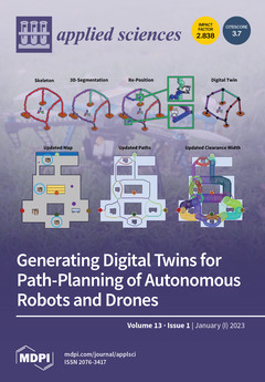
A digital twin describes the virtual presentation of a real process. Designing suitable digital twins for the path planning of autonomous robots or drones is often challenging due to a large number of different dynamic environments and multi-task and agent systems. In this work, homotopic shrinking is used to generate the digital twin, which can be used to extract all possible path proposals. Such a deterministic path algorithm can flexibly respond to changing environmental conditions and consider multiple tasks simultaneously for path generation. The method is tested on 2D and 3D maps with different tasks, obstacles, and multiple robots. Finally, it was shown that the environment for the digital twin can be reduced to reasonable paths by constrained shrinking, both for real 2D maps and for complex virtual 2D and 3D maps. View this paper
  • Issues are regarded as officially published after their release is announced to the table of contents alert mailing list.
  • You may sign up for e-mail alerts to receive table of contents of newly released issues.
  • PDF is the official format for papers published in both, html and pdf forms. To view the papers in pdf format, click on the "PDF Full-text" link, and use the free Adobe Reader to open them.
Order results
Result details
Section
Select all
Export citation of selected articles as:
23 pages, 1653 KiB  
Review
Control System Design and Methods for Collaborative Robots: Review
by Ayesha Hameed, Andrzej Ordys, Jakub Możaryn and Anna Sibilska-Mroziewicz
Appl. Sci. 2023, 13(1), 675; https://doi.org/10.3390/app13010675 - 3 Jan 2023
Cited by 17 | Viewed by 9466
Abstract
Collaborative robots cooperate with humans to assist them in undertaking simple-to-complex tasks in several fields, including industry, education, agriculture, healthcare services, security, and space exploration. These robots play a vital role in the revolution of Industry 4.0, which defines new standards of manufacturing [...] Read more.
Collaborative robots cooperate with humans to assist them in undertaking simple-to-complex tasks in several fields, including industry, education, agriculture, healthcare services, security, and space exploration. These robots play a vital role in the revolution of Industry 4.0, which defines new standards of manufacturing and the organization of products in the industry. Incorporating collaborative robots in the workspace improves efficiency, but it also introduces several safety risks. Effective safety measures then become indispensable to ensure safe and robust interaction. This paper presents the review of low-level control methodologies of a collaborative robot to assess the current status of human–robot collaboration over the last decade. First, we discuss the classification of human–robot collaboration, architectures of systems and the complex requirements on control strategies. The most commonly used control approaches were presented and discussed. Several methods of control, reported in industrial applications, are elaborated upon with a prime focus on HR-collaborative assembly operations. Since the physical HRC is a critical control problem for the co-manipulation task, this article identifies key control challenges such as the prediction of human intentions, safety, and human-caused disturbances in motion synchronization; the proposed solutions were analyzed afterwards. The discussion at the end of the paper summarizes the features of the control systems that should be incorporated within the systematic framework to allow the execution of a robotic task from global task planning to low-level control implementation for safe and robust interactions. Full article
(This article belongs to the Section Computing and Artificial Intelligence)
Show Figures

Figure 1

Figure 1
<p>Development of collaborative robotic system.</p>
Full article ">Figure 2
<p>Classification of human–robot interactions.</p>
Full article ">Figure 3
<p>Block diagram of collaborative control architecture.</p>
Full article ">Figure 4
<p>Interactive collaborative control framework.</p>
Full article ">Figure 5
<p>Force profiles of collision occurrence.</p>
Full article ">Figure 6
<p>Controller layout for SEA robots.</p>
Full article ">Figure 7
<p>Simplified diagram for an admittance-based collaborative task control.</p>
Full article ">Figure 8
<p>Invariance control architecture.</p>
Full article ">Figure 9
<p>Experimental setup at WUT.</p>
Full article ">
13 pages, 5140 KiB  
Article
Deep Image Clustering Based on Label Similarity and Maximizing Mutual Information across Views
by Feng Peng and Kai Li
Appl. Sci. 2023, 13(1), 674; https://doi.org/10.3390/app13010674 - 3 Jan 2023
Viewed by 3739
Abstract
Most existing deep image clustering methods use only class-level representations for clustering. However, the class-level representation alone is not sufficient to describe the differences between images belonging to the same cluster. This may lead to high intra-class representation differences, which will harm the [...] Read more.
Most existing deep image clustering methods use only class-level representations for clustering. However, the class-level representation alone is not sufficient to describe the differences between images belonging to the same cluster. This may lead to high intra-class representation differences, which will harm the clustering performance. To address this problem, this paper proposes a clustering model named Deep Image Clustering based on Label Similarity and Maximizing Mutual Information Across Views (DCSM). DCSM consists of a backbone network, class-level and instance-level mapping block. The class-level mapping block learns discriminative class-level features by selecting similar (dissimilar) pairs of samples. The proposed extended mutual information is to maximize the mutual information between features extracted from views that were obtained by using data augmentation on the same image and as a constraint on the instance-level mapping block. This forces the instance-level mapping block to capture high-level features that affect multiple views of the same image, thus reducing intra-class differences. Four representative datasets are selected for our experiments, and the results show that the proposed model is superior to the current advanced image clustering models. Full article
(This article belongs to the Special Issue Algorithms and Applications of Multi-View Information Clustering)
Show Figures

Figure 1

Figure 1
<p>Model Overview. The original image and its transformed image are regarded as a pair of inputs to learn class-level (C-block) and instance-level (IR-block) representations using a shared deep neural network. The similarity matrix is generated from the class-level feature similarity relationship of the transformed images, and the target matrix is generated using K-means in the original image class-level feature space to guide the similarity matrix. Cluster standard samples are selected according to the threshold to modify the network parameters. The discriminator network estimates the mutual information of local-global and local-local representations, respectively.</p>
Full article ">Figure 2
<p>Confusion matrixes of the cluster results. (<b>a</b>,<b>b</b>) represent the clustering results on MNIST and Imagenet10 datasets, respectively.</p>
Full article ">Figure 3
<p>Visualization of the class−level representations for different training stages of the proposed DCSM on the Imagenet10 datasets. (<b>a</b>) Initial stage of DCSM, (<b>b</b>) Middle stage of DCSM and (<b>c</b>) Final stage of DCSM.</p>
Full article ">Figure 4
<p>Clustering performance under different thresholds and <span class="html-italic">z</span>. (<b>a</b>) Impact of threshold. (<b>b</b>) The dimensional impact of <span class="html-italic">z</span>.</p>
Full article ">
14 pages, 1937 KiB  
Article
Research on Efficient Construction Paths for Intelligent Coal Mines in China from the Configuration Perspective
by Xiaofang Yuan, Yutong Wu, Linhui Sun and Xinping Wang
Appl. Sci. 2023, 13(1), 673; https://doi.org/10.3390/app13010673 - 3 Jan 2023
Cited by 23 | Viewed by 3733
Abstract
The intelligent transformation of coal mines is an inevitable choice to promote the green transformation of energy and to achieve safety and efficiency in the industry. Exploring the path of its efficient construction is the key to realizing the construction of intelligent coal [...] Read more.
The intelligent transformation of coal mines is an inevitable choice to promote the green transformation of energy and to achieve safety and efficiency in the industry. Exploring the path of its efficient construction is the key to realizing the construction of intelligent coal mines in China. To analyze the configuration paths for the efficient construction of intelligent coal mines, 17 typical coal-producing provinces in China were used as the research object of a fuzzy set qualitative comparative analysis (fsQCA), and five conditional variables, namely research funds, technical talent, government importance degree, national demonstration, and basic resource support, were selected from four levels (technology, organization, environment, and resources) based on relevant national data from 2019–2021, and multiple configurations as well as multiple driving paths for the construction of intelligent coal mines were discussed. We found that there are three configuration paths that will enable the construction of intelligent coal mines: a technology-driven path under the government’s supervision, a path jointly driven by three-prongs, and a policy-driven path under the resource priority. The critical importance of the government is the common factor among the three driving modes. These research results can provide useful construction ideas for the construction of intelligent coal mines in different regions and enable provincial governments to carry out strategic combination actions according to local conditions to contribute to the efficient construction of intelligent coal mines and the green transformation of energy across the country. Full article
Show Figures

Figure 1

Figure 1
<p>Analysis framework of factors influencing the construction of intelligent coal mines.</p>
Full article ">Figure 2
<p>Explanatory cases of three configurations.</p>
Full article ">
22 pages, 7200 KiB  
Article
AC Electric Powertrain without Power Electronics for Future Hybrid Electric Aircrafts: Architecture, Design and Stability Analysis
by Alexandre Richard, Xavier Roboam, Florent Rougier, Nicolas Roux and Hubert Piquet
Appl. Sci. 2023, 13(1), 672; https://doi.org/10.3390/app13010672 - 3 Jan 2023
Cited by 2 | Viewed by 1837
Abstract
This paper proposes an electric powertrain architecture for future hybrid electric aircrafts which structure is only composed of permanent magnet synchronous machines for both generators (PMSG) and motors (PMSM). The direct connection through an AC bus of a PMSG with one or several [...] Read more.
This paper proposes an electric powertrain architecture for future hybrid electric aircrafts which structure is only composed of permanent magnet synchronous machines for both generators (PMSG) and motors (PMSM). The direct connection through an AC bus of a PMSG with one or several PMSMs involves the suppression of power electronics usually embedded in electric or hybrid electric powertrains. The idea is clearly to simplify the architecture and to significantly reduce the weight of propulsive device, “weight being the prime enemy in aeronautics”. However, the connection between power generation and propulsion devices through power electronics converters offers degrees of freedom allowing to control and stabilize the whole system. Contrarily, the direct connection between synchronous machines (PMSG-PMSM) sets a rigid link with non-linear behavior between both devices, causing complex stability issues that are analyzed. For that purpose, after having discussed the advantages and drawbacks of this powertrain by comparison with classical architectures, including power electronics, a set of models (analytic and simulation) and analysis tools (root locus, transient time simulation) is proposed. They are used in a theoretical approach to emphasize the stability issue and to assess parameter sensitivity. A reduced power scale test bench with a single-motor AC powertrain is presented: together with circuit simulation models, it is used to compare and validate the theoretical analysis results. Full article
(This article belongs to the Special Issue Aerospace Vehicle Design under Uncertainties)
Show Figures

Figure 1

Figure 1
<p>Several topologies for the powertrain: (<b>a</b>) with power electronics coupling; (<b>b</b>) single-motor “power electronic-less” coupling; (<b>c</b>) multi-motor “power electronic-less” coupling.</p>
Full article ">Figure 2
<p>Two example of architectures (here with six propellers) with direct AC coupling between generators and motors.</p>
Full article ">Figure 3
<p>Park’s reference frames: (<b>a</b>) generator voltage and current vectors in the generator reference frame (<span class="html-italic">d<sub>g</sub></span>,<span class="html-italic">q<sub>g</sub></span>); (<b>b</b>) motor voltage and current vectors in the motor reference frame (<span class="html-italic">d<sub>m</sub></span>,<span class="html-italic">q<sub>m</sub></span>); (<b>c</b>) generator and motor voltage and current vectors with phase shift in the generator reference frame (<span class="html-italic">d<sub>g</sub></span>,<span class="html-italic">q<sub>g</sub></span>).</p>
Full article ">Figure 4
<p>IP speed control of the gas turbine—generator association.</p>
Full article ">Figure 5
<p>Comparison of time simulations between the analytic state model simulated on Matlab Simulink (red curves) and the circuit simulation on Saber (blue curves).</p>
Full article ">Figure 6
<p>Reduced power scale test bench for AC powertrain functional emulation.</p>
Full article ">Figure 7
<p>Small-signal model-based root locus with respect to the generator speed (blue crosses) with a bandwidth of 1 Hz for the generator speed control. Dashed lines illustrate iso-values of system damping (linear dashed lines), and iso-values of system angular frequency (horizontal dashed lines), the red line indicate the limit between stable and unstable zone: the ordinates axe.</p>
Full article ">Figure 8
<p>Time simulation with respect to variable stages of the generator speed with a bandwidth of 1 Hz for the generator speed control.</p>
Full article ">Figure 9
<p>Experimental test with respect to variable stages of the generator speed with a bandwidth of 1 Hz for the generator speed control.</p>
Full article ">Figure 10
<p>Small-signal model-based root locus with respect to the generator speed (blue crosses) with a bandwidth of 0.9 Hz for the gas turbine speed control.</p>
Full article ">Figure 11
<p>Time simulation with respect to variable stages of the generator speed with a bandwidth of 0.9 Hz for the gas turbine speed control.</p>
Full article ">Figure 12
<p>Experimental test with respect to variable stages of the generator speed with a bandwidth of 0.9 Hz for the gas turbine speed control.</p>
Full article ">Figure 13
<p>Small-signal model-based root locus with respect to the gas turbine control dynamic (blue crosses) with a bandwidth varying between 0.5 and 50 Hz (with a constant speed of 400 rpm).</p>
Full article ">Figure 14
<p>Small-signal model-based root locus analysis for coupled parametric modifications with a bandwidth of 1 Hz for the generator speed control and with coupled modifications of electric and mechanical parameters.</p>
Full article ">Figure 15
<p>Time simulation analysis for coupled parametric modifications with a bandwidth of 1 Hz for the generator speed control and with coupled modifications of electric and mechanical parameters.</p>
Full article ">Figure 16
<p>Small-signal model-based root locus analysis for the previous coupled parametric modifications with a bandwidth of 1 Hz for the generator speed control and with coupled modifications of electric and mechanical parameters.</p>
Full article ">Figure 17
<p>Time simulation result of the stability analysis for the previous coupled parametric modification with a bandwidth of 1 Hz for the generator speed control and with coupled modifications of electric and mechanical parameters.</p>
Full article ">
14 pages, 4521 KiB  
Article
Three-Dimensional Numerical Modeling of Artificially Freezing Ground in Metro Station Construction
by Bo Wang, Jun Hu, Xiaoqi Lin and Hui Zeng
Appl. Sci. 2023, 13(1), 671; https://doi.org/10.3390/app13010671 - 3 Jan 2023
Viewed by 2014
Abstract
In this study, the engineering background of No. 2 complex connecting passage of Binhu Road Station/Jinhu Square Station of Nanning Metro Line 3 is investigated, where the artificial ground freezing technique is adopted. A three-dimensional finite element model is established to investigate the [...] Read more.
In this study, the engineering background of No. 2 complex connecting passage of Binhu Road Station/Jinhu Square Station of Nanning Metro Line 3 is investigated, where the artificial ground freezing technique is adopted. A three-dimensional finite element model is established to investigate the temperature development of the frozen soil curtain, with a simulation of the dynamic evolution of the frosted soil curtain. The finite element model is validated by comparing the overall trend of the measured temperature value and the resulting temperature value, which are roughly the same. According to the design scheme, the weakest part of the whole frozen soil curtain is the top of the bell mouth where the downhole tunnel intersects the connecting passage. It is recommended to make a row of smaller freezing holes to enhance the freezing effect in this area. The thickness of the frozen soil curtain reached 1.75 m or more, indicating that the whole frozen soil curtain meets the design requirements and shows the right features for excavation construction. After freezing for 40 days, the average thickness of the frozen soil curtain is 2.4 m, indicating that the freezing effect meets the design requirements. The project can be successfully carried out, which suggests that the underneath passage construction is feasible. As a result, the results of the numerical model are applicable for comparable projects using artificially freezing ground in metro station construction. Full article
(This article belongs to the Special Issue State-of-the-Art Earth Sciences and Geography in China)
Show Figures

Figure 1

Figure 1
<p>Elevation profile of the connecting passage (diameter of tunnel: 6.3 m; center to center distance: 15.3 m).</p>
Full article ">Figure 2
<p>Layout of freezing holes on the machine room side.</p>
Full article ">Figure 3
<p>Contralateral freezing hole layout.</p>
Full article ">Figure 4
<p>Mesh size and geometric size of the numerical model. (<b>a</b>) mesh and geometric size of the model; (<b>b</b>) distribution of freeze pipes.</p>
Full article ">Figure 5
<p>Comparison between simulated results and site data. (<b>a</b>) Measuring point 1, (<b>b</b>) measuring point 2.</p>
Full article ">Figure 6
<p>Freezing curtain under 40-day freezing. (<b>a</b>) x = −3.0 m, (<b>b</b>) x = −6.0 m, (<b>c</b>) x = −9.0 m, (<b>d</b>) x = −12.0 m.</p>
Full article ">Figure 7
<p>Isotherms for −1 and −10 °C for various freezing times. (<b>a</b>) Actively frozen for 6 days, (<b>b</b>) actively frozen for 8 days, (<b>c</b>) actively frozen for 10 days, (<b>d</b>) actively frozen for 12 days, (<b>e</b>) actively frozen for 14 days.</p>
Full article ">Figure 7 Cont.
<p>Isotherms for −1 and −10 °C for various freezing times. (<b>a</b>) Actively frozen for 6 days, (<b>b</b>) actively frozen for 8 days, (<b>c</b>) actively frozen for 10 days, (<b>d</b>) actively frozen for 12 days, (<b>e</b>) actively frozen for 14 days.</p>
Full article ">Figure 8
<p>Temperature changes at points C1–C7 against freezing time. (<b>a</b>) C1 path, (<b>b</b>) C2 path, (<b>c</b>) C3 path, (<b>d</b>) C4 path, (<b>e</b>) C5 path, (<b>f</b>) C6 path, (<b>g</b>) C7 path.</p>
Full article ">Figure 8 Cont.
<p>Temperature changes at points C1–C7 against freezing time. (<b>a</b>) C1 path, (<b>b</b>) C2 path, (<b>c</b>) C3 path, (<b>d</b>) C4 path, (<b>e</b>) C5 path, (<b>f</b>) C6 path, (<b>g</b>) C7 path.</p>
Full article ">
21 pages, 6138 KiB  
Article
ReconTraj4Drones: A Framework for the Reconstruction and Semantic Modeling of UAVs’ Trajectories on MovingPandas
by Konstantinos Kotis and Andreas Soularidis
Appl. Sci. 2023, 13(1), 670; https://doi.org/10.3390/app13010670 - 3 Jan 2023
Cited by 1 | Viewed by 2764
Abstract
Unmanned aerial vehicles (UAVs), also known as drones, are important for several application domains, such as the military, agriculture, cultural heritage documentation, surveillance, and the delivery of goods/products/services. A drone’s trajectory can be enriched with external and heterogeneous data beyond latitude, longitude, and [...] Read more.
Unmanned aerial vehicles (UAVs), also known as drones, are important for several application domains, such as the military, agriculture, cultural heritage documentation, surveillance, and the delivery of goods/products/services. A drone’s trajectory can be enriched with external and heterogeneous data beyond latitude, longitude, and timestamp to create its semantic trajectory, providing meaningful and contextual information on its movement data, enabling decision makers to acquire meaningful and enriched contextual information about the current situation in the field of its operation and eventually supporting simulations and predictions of high-level critical events. In this paper, we present an ontology-based, tool-supported framework for the reconstruction, modeling, and enrichment of drones’ semantic trajectories. This framework extends MovingPandas, a widely used and open-source trajectory analytics and visualization tool. The presented research extends our preliminary work on drones’ semantic trajectories by contributing (a) an updated methodology for the reconstruction of drones’ trajectories from geo-tagged photos taken by drones during their flights in cases in which flight plans and/or real-time movement data have been lost or corrupted; (b) an enrichment of the reconstructed trajectories with external data; (c) the semantic annotation of the enriched trajectories based on a related ontology; and (d) the use of SPARQL queries to analyze and retrieve knowledge related to the flight of a drone and the field of operations (context). An evaluation of the presented framework, namely, ReconTraj4Drones, was conducted against several criteria, using real and open datasets. Full article
(This article belongs to the Special Issue Unmanned Aerial Vehicles (UAVs) and Their Applications)
Show Figures

Figure 1

Figure 1
<p>Drone’s flight area of interest in the presented scenario, taking photos (blue pins) during a cultural heritage documentation mission (green and red pins represent the start and the end of the flight).</p>
Full article ">Figure 2
<p>Workflow of the trajectory reconstruction, semantic annotation, and analytics.</p>
Full article ">Figure 3
<p>High-level architectural design of ReconTraj4Drones framework.</p>
Full article ">Figure 4
<p>The form of a DataFrame after the trajectory reconstruction process.</p>
Full article ">Figure 5
<p>Returned data from Meteostat for a given latitude, longitude, timestamp, and altitude.</p>
Full article ">Figure 6
<p>Trajectory interactive visualization. (<b>a</b>) Visualization of the total number of points that make up the trajectory; (<b>b</b>) visualization of a percentage of points set by the user.</p>
Full article ">Figure 7
<p>Basic concepts and relations of the Onto4drone ontology.</p>
Full article ">Figure 8
<p>A trajectory reconstructed from extracted data/metadata.</p>
Full article ">Figure 9
<p>Weather data obtained using open Web services.</p>
Full article ">Figure 10
<p>Point of interest data obtained using open Web services.</p>
Full article ">Figure 11
<p>Trajectory segments based on distance.</p>
Full article ">Figure 12
<p>Detected stops of evaluated trajectories.</p>
Full article ">Figure 13
<p>Visualization of a segmented trajectory.</p>
Full article ">Figure 14
<p>Interactive visualization of a trajectory. (<b>a</b>) Visualization of information contained in each point of the trajectory; (<b>b</b>) visualization of the data contained in a stop area of the trajectory.</p>
Full article ">Figure 15
<p>A point in the evaluated trajectory, along with weather data, in RDF.</p>
Full article ">Figure 16
<p>An example SPARQL query defined by user in Jupyter notebook environment.</p>
Full article ">
17 pages, 10044 KiB  
Article
Preliminary Study for Smoke Color Classification of Combustibles Using the Distribution of Light Scattering by Smoke Particles
by Hyo-Yeon Jang and Cheol-Hong Hwang
Appl. Sci. 2023, 13(1), 669; https://doi.org/10.3390/app13010669 - 3 Jan 2023
Cited by 7 | Viewed by 2542
Abstract
Photoelectric smoke detectors are used for early detection of building fires, and sensitivity adjustment is generally performed using white smoke generated by the burning of filter paper. Therefore, when black smoke of the same concentration is introduced, the detector is often not activated. [...] Read more.
Photoelectric smoke detectors are used for early detection of building fires, and sensitivity adjustment is generally performed using white smoke generated by the burning of filter paper. Therefore, when black smoke of the same concentration is introduced, the detector is often not activated. To address this problem, differences in the distribution of light scattered by smoke of various colors were analyzed. A light-scattering chamber with a light-receiving unit for various scattering angles was constructed to measure the scattered light generated inside the chamber of the smoke detector. The light scattering distribution was measured for smoke generated from three combustibles—filter paper (white smoke), kerosene (black smoke), and polyurethane (gray-black smoke)—and three analysis criteria were applied. By identifying a section where the measured values were concentrated for a specific analysis criterion and scattering angle, it was confirmed that some combustibles can be distinguished. Specifically, criterion III, a probabilistic section, was presented to determine which combustible smoke particles were close by applying the proposed section in a complex manner. A preliminary study was conducted to evaluate a methodology for the color classification of smoke particles flowing into a smoke detector chamber; this can be utilized as a foundation for determining optical properties. Full article
(This article belongs to the Special Issue Advanced Analysis and Technology in Fire Science and Engineering)
Show Figures

Figure 1

Figure 1
<p>(<b>a</b>) Photograph and (<b>b</b>) schematics of test duct and light scattering chamber (LSC).</p>
Full article ">Figure 2
<p>Schematics of optical characteristics: (<b>a</b>) schematic of light scattering, absorbed and diffracted for smoke particle; (<b>b</b>) schematic of forward and backward scattering inside of a multiple angles chamber.</p>
Full article ">Figure 3
<p>Comparison of experimental data about <math display="inline"><semantics> <mrow> <msub> <mi>I</mi> <mi>i</mi> </msub> <mo>−</mo> <msubsup> <mi>I</mi> <mi>i</mi> <mn>0</mn> </msubsup> <mo> </mo> </mrow> </semantics></math>at LSC on smoke particles.</p>
Full article ">Figure 4
<p>Comparison of experimental data on <math display="inline"><semantics> <mrow> <msub> <mi>I</mi> <mi>i</mi> </msub> <mo>/</mo> <msubsup> <mi>I</mi> <mi>i</mi> <mn>0</mn> </msubsup> <mo>,</mo> </mrow> </semantics></math> measured at LSC on smoke particles.</p>
Full article ">Figure 5
<p>The difference in the distribution of scattering intensity from smoke particles of combustibles.</p>
Full article ">Figure 6
<p>Detection of optical density through a smoke detector for each combustible.</p>
Full article ">Figure 7
<p>Comparison of results for the distribution of optical analysis criteria for the primary ratio according to the scattering angles (<span class="html-italic">I</span> = 150°).</p>
Full article ">Figure 8
<p>Distribution of ratios of light extinction and total light scattering according to combustibles.</p>
Full article ">Figure 9
<p>Example of insufficient results according to criterion I for the combustibles inside the chamber.</p>
Full article ">Figure 10
<p>Comparison of results according to criterion II for the combustibles inside the chamber.</p>
Full article ">Figure 11
<p>Comparison of results according to criterion III for the combustibles inside the chamber.</p>
Full article ">
18 pages, 4429 KiB  
Article
A Two-Stage Rolling Bearing Weak Fault Feature Extraction Method Combining Adaptive Morphological Filter with Frequency Band Selection Strategy
by Jun Li, Hongchao Wang, Simin Li, Liang Chen and Qiqian Dang
Appl. Sci. 2023, 13(1), 668; https://doi.org/10.3390/app13010668 - 3 Jan 2023
Cited by 1 | Viewed by 1778
Abstract
To extract the weak fault features hidden in strong background interference in the event of the early failure of rolling bearings, a two-stage based method is proposed. The broadband noise elimination ability of an adaptive morphological filter (AMF) and the superior capability of [...] Read more.
To extract the weak fault features hidden in strong background interference in the event of the early failure of rolling bearings, a two-stage based method is proposed. The broadband noise elimination ability of an adaptive morphological filter (AMF) and the superior capability of a frequency band selection (FBS) strategy for fault transient location identification are comprehensively utilized by the proposed method. Firstly, the AMF with a simple theory and high calculation efficiency is used as a preprocessing program to enhance the fault transient features. Then, the proposed FBS strategy based on the sparsity index (SI) is utilized to further handle the filtered signal processed by the AMF. Finally, the constructed optimum bandpass filter based on the analysis result of the FBS is used to further filter the handled signal processed by AMF and envelope spectral analysis is applied on the last filtered signal to realize the ideal fault feature extraction effect. Compared with the other traditional FBS methods based on kurtosis or the other index, the proposed FBS strategy based on SI has strong robustness to noise. One experimental signal and one engineering vibration signal are used, respectively, to verify the feasibility of the proposed method. Full article
(This article belongs to the Special Issue Active Vibration and Noise Control)
Show Figures

Figure 1

Figure 1
<p>Illustration of designing SEs of MF.</p>
Full article ">Figure 2
<p>The filter result of the rolling bearing simulated signal based the proposed AMF. (<b>a</b>) Periodic impulses. (<b>b</b>) Harmonic components. (<b>c</b>) Random impulses. (<b>d</b>) White noise. (<b>e</b>) Mixed signal. (<b>f</b>) Envelope spectral of the signal shown in (<b>e</b>). (<b>g</b>) The filtered signal of the mixed signal shown in (<b>e</b>) using the proposed AMF. (<b>h</b>) Envelope spectral of the signal as shown (<b>g</b>).</p>
Full article ">Figure 2 Cont.
<p>The filter result of the rolling bearing simulated signal based the proposed AMF. (<b>a</b>) Periodic impulses. (<b>b</b>) Harmonic components. (<b>c</b>) Random impulses. (<b>d</b>) White noise. (<b>e</b>) Mixed signal. (<b>f</b>) Envelope spectral of the signal shown in (<b>e</b>). (<b>g</b>) The filtered signal of the mixed signal shown in (<b>e</b>) using the proposed AMF. (<b>h</b>) Envelope spectral of the signal as shown (<b>g</b>).</p>
Full article ">Figure 3
<p>The production of three of the filter bands.</p>
Full article ">Figure 4
<p>Five signals with their four indexes. (<b>a</b>) Five signals. (<b>b</b>) Four indexes corresponding to the five signals as shown in (<b>a</b>).</p>
Full article ">Figure 5
<p>Flow chart of the proposed method.</p>
Full article ">Figure 6
<p>The test rig.</p>
Full article ">Figure 7
<p>Experiment verification of the proposed method. (<b>a</b>) The original vibration signal of the experimental bearing at its early weak fault stage. (<b>b</b>) Envelope spectral of the signal shown in (<b>a</b>). (<b>c</b>) The filtered signal of the signal shown in (<b>a</b>) using AMF. (<b>d</b>) Envelope spectral of the signal shown in (<b>c</b>). (<b>e</b>) Analysis result of the signal shown in (<b>c</b>) using the proposed FBS method. (<b>f</b>) Envelope of the filtered signal of the signal shown in (<b>c</b>) using the proposed FBS method. (<b>g</b>) FFT of the signal shown in (<b>f</b>).</p>
Full article ">Figure 7 Cont.
<p>Experiment verification of the proposed method. (<b>a</b>) The original vibration signal of the experimental bearing at its early weak fault stage. (<b>b</b>) Envelope spectral of the signal shown in (<b>a</b>). (<b>c</b>) The filtered signal of the signal shown in (<b>a</b>) using AMF. (<b>d</b>) Envelope spectral of the signal shown in (<b>c</b>). (<b>e</b>) Analysis result of the signal shown in (<b>c</b>) using the proposed FBS method. (<b>f</b>) Envelope of the filtered signal of the signal shown in (<b>c</b>) using the proposed FBS method. (<b>g</b>) FFT of the signal shown in (<b>f</b>).</p>
Full article ">Figure 8
<p>The monitored engineering object.</p>
Full article ">Figure 9
<p>The actual faulty component of the engineering bearing.</p>
Full article ">Figure 10
<p>Engineering verification of the proposed method. (<b>a</b>) The original vibration signal of engineering bearing. (<b>b</b>) Envelope spectral of the signal shown in (<b>a</b>). (<b>c</b>) The filtered signal of the signal shown in (<b>a</b>) using the proposed AMF. (<b>d</b>) Envelope spectral of the signal shown in (<b>c</b>). (<b>e</b>) Analysis result of the signal shown in (<b>c</b>) using the proposed FBS method. (<b>f</b>) Envelope of the filtered signal of the signal shown in (<b>c</b>) using the proposed FBS method. (<b>g</b>) FFT of the signal shown in (<b>f</b>).</p>
Full article ">Figure 10 Cont.
<p>Engineering verification of the proposed method. (<b>a</b>) The original vibration signal of engineering bearing. (<b>b</b>) Envelope spectral of the signal shown in (<b>a</b>). (<b>c</b>) The filtered signal of the signal shown in (<b>a</b>) using the proposed AMF. (<b>d</b>) Envelope spectral of the signal shown in (<b>c</b>). (<b>e</b>) Analysis result of the signal shown in (<b>c</b>) using the proposed FBS method. (<b>f</b>) Envelope of the filtered signal of the signal shown in (<b>c</b>) using the proposed FBS method. (<b>g</b>) FFT of the signal shown in (<b>f</b>).</p>
Full article ">Figure 11
<p>The experimental signal shown in <a href="#applsci-13-00668-f007" class="html-fig">Figure 7</a>a using fast Mkurtogram. (<b>a</b>) FDMK. (<b>b</b>) Waveform of the filtered signal. (<b>c</b>) The envelope spectral of (<b>b</b>).</p>
Full article ">Figure 12
<p>The engineering signal shown in <a href="#applsci-13-00668-f009" class="html-fig">Figure 9</a> using fast Mkurtogram. (<b>a</b>) FDMK. (<b>b</b>) Waveform of the filtered signal. (<b>c</b>) The envelope spectral of (<b>b</b>).</p>
Full article ">Figure 13
<p>The experimental signal shown in <a href="#applsci-13-00668-f007" class="html-fig">Figure 7</a>a using the proposed method in [<a href="#B48-applsci-13-00668" class="html-bibr">48</a>]. (<b>a</b>) Pareto front. (<b>b</b>) Distribution of the Pareto set. (<b>c</b>) Filtered signal. (<b>d</b>) The envelope spectral of (<b>c</b>).</p>
Full article ">
11 pages, 261 KiB  
Article
Reliability of the Polygraphic Home Sleep Test for OSA Determined by the Severity and Pattern Changes of Two Consecutive Examinations
by Renáta Rozgonyi, József Janszky, Norbert Kovács and Béla Faludi
Appl. Sci. 2023, 13(1), 667; https://doi.org/10.3390/app13010667 - 3 Jan 2023
Viewed by 1477
Abstract
Diagnosis and effective treatment of obstructive sleep apnea syndrome (OSA) in adults is an important health priority. Home respiratory polygraphy is a cost-effective alternative to polysomnography in OSA. The aim of this study was to investigate the variability of two consecutive home respiratory [...] Read more.
Diagnosis and effective treatment of obstructive sleep apnea syndrome (OSA) in adults is an important health priority. Home respiratory polygraphy is a cost-effective alternative to polysomnography in OSA. The aim of this study was to investigate the variability of two consecutive home respiratory polygraphic examinations by comparing the severity characteristics and pattern (supine dominant, continuous, etc.) variability. We examined 100 patients with clinically suspected OSA on two consecutive nights by home respiratory polygraphy. The correlation of time in bed (TIB), apnea-hypopnea index (AHI), oxygen desaturation index (ODI), and T90 of the two examinations were compared by the Pearson test. The severity ranks and nocturnal apnea patterns of the two periods were compared using Spearman and Wilcoxon tests. Pearson’s correlations represented a strong correlation of the AHI, ODI, and T90, but only moderate for TIB. The severity-specific correlation was the highest for AHI in the severe group. Out of 100 pairs of polygraphic examinations, 25 cases showed change in the severity ranking (decreased in 11, increased in 14); 15 cases showed a change in the polygraphic pattern (supine, non-supine, etc.), with severity change in 6 cases. Therapy change based on the second examination was initiated in 6 cases. Our results revealed a good intra-individual correlation between the severity grades of the two nights, with the highest value in the severe cases. In some cases, the nightly variation in the polygraphic pattern may explain the change in the severity. From a therapeutic point of view, the low number of severity changes between moderate and severe groups revealed good reliability. Full article
(This article belongs to the Special Issue Obstructive Sleep Apnoea Syndrome and Its Management)
8 pages, 2818 KiB  
Communication
Biomechanical Rationale for a Novel Implant Design Reducing Stress on Buccal Bone
by Annika Schulz, Virgilia Klär, Tanja Grobecker-Karl and Matthias Karl
Appl. Sci. 2023, 13(1), 666; https://doi.org/10.3390/app13010666 - 3 Jan 2023
Cited by 4 | Viewed by 1610
Abstract
Modern implant designs should allow for adequate primary stability but limit mechanical stress on buccal bone in order to prevent initial marginal bone loss. A dental implant characterized by a shift in core diameter and thread geometry was evaluated. Polyurethane foam was used [...] Read more.
Modern implant designs should allow for adequate primary stability but limit mechanical stress on buccal bone in order to prevent initial marginal bone loss. A dental implant characterized by a shift in core diameter and thread geometry was evaluated. Polyurethane foam was used as bone surrogate material and implant placement was performed measuring insertion torque and strain development on buccal bone using strain gauges as well as primary stability by using damping capacity assessments. An existing tapered bone-level implant was used as a control while the novel experimental implant described above (n = 10) was used in the test group. Statistical analysis was based on t-tests (α = 0.05). Both the maximum insertion torque (p = 0.0016) and maximum strain development in buccal bone (p = 0.1069) were greater in control implants as compared to the novel implant design. Moreover, in the control group, these were reached at a significantly later timepoint of the insertion process, i.e., when the implant was almost fully seated (maximum insertion torque p = 0.0001, maximum strain development p < 0.00001). The final insertion torque (p < 0.00001) and final strain development (p = 0.0137) were significantly lower in the novel implant design while the primary stability of both implant types did not differ significantly (p = 0.219). The novel implant design allowed for a greater undersizing of osteotomies while not mechanically overstressing buccal bone. Comparable primary stability was obtained from trabecular bone instead of compressing cortical bone as occurs in conventional, existing tapered implant designs. Full article
(This article belongs to the Section Applied Dentistry and Oral Sciences)
Show Figures

Figure 1

Figure 1
<p>Bone-level implant types used in this study comprising Straumann BLT 4.1 × 10 mm (<b>a</b>) and AlfaGate 4.3 × 10 mm (<b>b</b>).</p>
Full article ">Figure 2
<p>Insertion of a novel design AlfaGate implant (<b>a</b>) and a Straumann BLT implant (<b>b</b>) into osteotomies created in laminated polyurethane foam simulating alveolar bone. Strain gauges were positioned on the buccal aspect of the bone with the sensing elements oriented in the horizontal direction for recording deformation of the material.</p>
Full article ">Figure 3
<p>Torque development over time during implant insertion for both groups investigated showing an overall torque increase with insertion depth for Straumann BLT while lower maximum torque was required in AlfaGate implants coinciding with the bulky central part of the implant passing the cortical plate.</p>
Full article ">Figure 4
<p>Strain development over time during implant insertion for both groups investigated with continuously increasing strain levels for Straumann BLT. Lower maximum strain was seen in AlfaGate implants coinciding with the bulky central part of the implant passing the cortical plate.</p>
Full article ">
14 pages, 4052 KiB  
Article
Comparison of Measurement Possibilities by Non-Invasive Reflectometric Sensors and Invasive Probes
by Magdalena Paśnikowska-Łukaszuk, Magda Wlazło-Ćwiklińska, Jarosław Zubrzycki and Zbigniew Suchorab
Appl. Sci. 2023, 13(1), 665; https://doi.org/10.3390/app13010665 - 3 Jan 2023
Cited by 3 | Viewed by 1722
Abstract
The measurement of the moisture content of building materials is of key importance both in the process of building structures and in their subsequent operation. In engineering practice, indirect techniques of moisture measurement, mainly, resistance and capacitive, are the most popular. The main [...] Read more.
The measurement of the moisture content of building materials is of key importance both in the process of building structures and in their subsequent operation. In engineering practice, indirect techniques of moisture measurement, mainly, resistance and capacitive, are the most popular. The main objective of this research work was to compare the classic TDR measurement technique to the non-invasive, surface TDR sensors. Moisture measurements were carried out on samples made of cellular concrete with density class of 400 and 600. These samples were moist to various degrees, from 0 to 69% (400 c.c.) and from 0 to 55 (600 c.c.). For each sample, five measurements were carried out. Both the RMSE and the expanded uncertainty values were more favorable for the TDR FP/mts probe and were consistent with the literature data. Compared to them, the measurement result for the 400 c.c. samples with the S1 probe was 154.6%, and that with the S2 probe was 87.03% of the values obtained with the invasive probe. When measuring the 600 c.c. samples, we found values of 122.16% for S1 and of 120.1% for S2 of those obtained with the invasive probe. The use of surface TDR sensors provided an easy and quick measurement without damaging the surface and structure of the tested material, as there was no need to introduce the probe actuators inside the tested material. Full article
(This article belongs to the Topic Advances in Non-Destructive Testing Methods)
Show Figures

Figure 1

Figure 1
<p>FP/mts TDR sensor applied in this research (ETest, Lublin, Poland).</p>
Full article ">Figure 2
<p>S1 non-invasive TDR sensor [<a href="#B42-applsci-13-00665" class="html-bibr">42</a>]. (<b>a</b>) Isometric view, (<b>b</b>) view from the bottom.</p>
Full article ">Figure 3
<p>S2 non-invasive TDR sensor [<a href="#B42-applsci-13-00665" class="html-bibr">42</a>]. (<b>a</b>) Isometric view, (<b>b</b>) view from the bottom.</p>
Full article ">Figure 4
<p>Relationship between the apparent permittivity reads determined with the use of the FP/mts invasive probe and the non-invasive probe and the moisture content of class 400 c.c. and 600 c.c. samples.</p>
Full article ">Figure 5
<p>Uncertainty dependence on material moisture: invasive, S1 and S2 sensor, 400 and 600 c.c. samples.</p>
Full article ">
13 pages, 6379 KiB  
Article
Pavement Structure Characteristics and Behaviour Analysis with Digital Image Correlation
by Ivana Barišić, Tihomir Dokšanović and Matija Zvonarić
Appl. Sci. 2023, 13(1), 664; https://doi.org/10.3390/app13010664 - 3 Jan 2023
Cited by 5 | Viewed by 1688
Abstract
Digital image correlation (DIC) is a method of point displacement measurement by an optical system. If two cameras are used for capturing the same point displacement, three-dimensional data are obtained using the 3D-DIC method. The areas of application of this method in pavement [...] Read more.
Digital image correlation (DIC) is a method of point displacement measurement by an optical system. If two cameras are used for capturing the same point displacement, three-dimensional data are obtained using the 3D-DIC method. The areas of application of this method in pavement construction are diverse, but it is mainly used for displacement monitoring during standard tests of the failure of specimens due to load application. Furthermore, DIC technology was used only for testing particular material characteristics and assuming their influence on the overall pavement system. Within this research, DIC was applied in two areas: defining material mechanical characteristics and analyses of pavement structure behaviour under cyclic loading. The scope of this research was to gain more insights into DIC’s potential application within pavement behaviour analyses, specifically on cement-bound granular material (CBGM) characterisation. Results from this study confirm the suitability of 3D-DIC technology for pavement material characterisation. Furthermore, it is shown that certain trends of material behaviour defined on the simple material level of each independent pavement layer will significantly differ when it is placed in the system, and this kind of complex analysis is possible by using 3D-DIC technology. Full article
(This article belongs to the Special Issue New Trends in Sustainable Geotechnics—Volume II)
Show Figures

Figure 1

Figure 1
<p>Grain size distribution of used natural aggregates.</p>
Full article ">Figure 2
<p>Pavement structure test setup.</p>
Full article ">Figure 3
<p>The 3D-DIC testing setup.</p>
Full article ">Figure 4
<p>CBGM specimen surface.</p>
Full article ">Figure 5
<p>Force–vertical displacement curves for selected samples of the CBGM with (<b>a</b>) 3%, (<b>b</b>) 5%, and (<b>c</b>) 7% cement content.</p>
Full article ">Figure 6
<p>Force–displacement envelopes for the pavement system with different CBGM layers.</p>
Full article ">Figure 7
<p>Vertical displacement at the end of each loading cycle.</p>
Full article ">Figure 8
<p>Displacement fields at the end of the 4th loading cycle for samples with various levels of cement.</p>
Full article ">
14 pages, 19559 KiB  
Review
Evaluation of the Efficacy of Probiotics Domiciliary Protocols for the Management of Periodontal Disease, in Adjunction of Non-Surgical Periodontal Therapy (NSPT): A Systematic Literature Review
by Andrea Butera, Elisa Folini, Saverio Cosola, Gianluca Russo, Andrea Scribante, Simone Gallo, Giulia Stablum, Giovanni Battista Menchini Fabris, Ugo Covani and Annamaria Genovesi
Appl. Sci. 2023, 13(1), 663; https://doi.org/10.3390/app13010663 - 3 Jan 2023
Cited by 9 | Viewed by 2602
Abstract
Introduction: Periodontitis is a multifactorial chronic inflammatory disease induced by a dysbiosis between the host and oral microbiota, which can compromise the host’s immune defenses and lead to the destruction of periodontal tissues. Despite the efficacy of non-surgical periodontal therapy (NSPT) as the [...] Read more.
Introduction: Periodontitis is a multifactorial chronic inflammatory disease induced by a dysbiosis between the host and oral microbiota, which can compromise the host’s immune defenses and lead to the destruction of periodontal tissues. Despite the efficacy of non-surgical periodontal therapy (NSPT) as the gold standard of periodontal treatment, its application can produce lower results due to anatomical and microbiological limitations. This systematic literature review was performed to assess the long-term efficacy of the effects of probiotics as an adjunct to NSPT compared to the control groups with follow-up of clinical, microbiological and immunological outcomes. Materials and methods: A literature review was conducted, considering manuscripts published from November 2016 to February 2022. The research question was formulated following the population, intervention, comparison and outcome strategies. Randomized controlled trials (RCT), systematic review and meta-analysis investigating the periodontal efficacy of domiciliary probiotic therapy in an adjunct to the mechanical therapy were included. Results: Regarding clinical outcomes, there is a reduction in periodontal probing depth (PPD), clinical attachments level (CAL), bleeding on probing (BoP) and plaque index (PI) for the test groups compared to the control groups in a short-term period. No differences were generally observed in the following indices over a period of more than 3 months for most studies considered. Conclusions: Weak evidence suggests that the use of probiotics as an adjunct to non-surgical periodontal therapy treatment may be able to show improvements in periodontal clinical parameters for up to 3 months. However, a significant and large heterogeneity of studies, along with the absence of long-term microbiological and immunological data, preclude any definitive conclusions. Full article
Show Figures

Figure 1

Figure 1
<p>Preferred Reporting Items for Systematic review and Meta-Analysis (PRISMA) flow diagram.</p>
Full article ">Figure 2
<p>Clinical case before (upper photograph) and after (lower photograph) non-surgical periodontal therapy with the adjunctive use of probiotics.</p>
Full article ">
9 pages, 2148 KiB  
Article
DFA-UNet: Efficient Railroad Image Segmentation
by Yan Zhang, Kefeng Li, Guangyuan Zhang, Zhenfang Zhu and Peng Wang
Appl. Sci. 2023, 13(1), 662; https://doi.org/10.3390/app13010662 - 3 Jan 2023
Cited by 8 | Viewed by 3799
Abstract
In computer vision technology, image segmentation is a significant technological advancement for the current problems of high-speed railroad image scene changes, low segmentation accuracy, and serious information loss. We propose a segmentation algorithm, DFA-UNet, based on an improved U-Net network architecture. The model [...] Read more.
In computer vision technology, image segmentation is a significant technological advancement for the current problems of high-speed railroad image scene changes, low segmentation accuracy, and serious information loss. We propose a segmentation algorithm, DFA-UNet, based on an improved U-Net network architecture. The model uses the same encoder–decoder structure as U-Net. To be able to extract image features efficiently and further integrate the weights of each channel feature, we propose to embed the DFA attention module in the encoder part of the model for the adaptive adjustment of feature map weights. We evaluated the performance of the model on the RailSem19 dataset. The results showed that our model showed improvements of 2.48%, 0.22%, 3.31%, 0.97%, and 2.2% in mIoU, F1-score, Accuracy, Precision, and Recall, respectively, compared with U-Net. The model can effectively achieve the segmentation of railroad images. Full article
(This article belongs to the Special Issue Applications of Video, Digital Image Processing and Deep Learning)
Show Figures

Figure 1

Figure 1
<p>Comparing our DFA (<b>e</b>) with U-Net (<b>a</b>), Stem Block (<b>b</b>), LKA (<b>c</b>), and PFC (<b>d</b>) designs used to extract the low-level semantic information from the input images.</p>
Full article ">Figure 2
<p>The framework of the GAMP block.</p>
Full article ">Figure 3
<p>DFA-UNet network architecture designs.</p>
Full article ">Figure 4
<p>MIoU performance on different models.</p>
Full article ">Figure 5
<p>Training loss on different models.</p>
Full article ">Figure 6
<p>Qualitative comparison results between DFA-Net and other models on rail segmentation datasets.</p>
Full article ">
12 pages, 23752 KiB  
Brief Report
Long-Term Clinical and Radiographic Analysis of Platform Matching and Platform Switching Implants in the Esthetic Zone: A Retrospective Cohort Study
by Andrea Raco, Bianca Di Murro, Pier Carmine Passarelli, Antonio D’Addona, Andrea Pilloni, Lorenzo Marini and Piero Papi
Appl. Sci. 2023, 13(1), 661; https://doi.org/10.3390/app13010661 - 3 Jan 2023
Cited by 1 | Viewed by 3788
Abstract
Background: The aims of this study are to retrospectively compare the clinical, radiographic and esthetic outcomes of platform switching (PS) and platform matching (PM) dental implants in the anterior maxilla after ≥ 10 years of functional loading. Methods: Marginal bone loss (MBL) levels [...] Read more.
Background: The aims of this study are to retrospectively compare the clinical, radiographic and esthetic outcomes of platform switching (PS) and platform matching (PM) dental implants in the anterior maxilla after ≥ 10 years of functional loading. Methods: Marginal bone loss (MBL) levels were recorded; furthermore, peri-implant clinical parameters (PPD, BOP, PI) were collected and the Pink and White Esthetic scores (PES/WES) were used to evaluate the esthetic outcomes. Wilcoxon signed rank tests were performed to compare collected parameters among the two groups, with a p-value < 0.05. Results: A final sample of 58 patients was enrolled in this study (PM implants = 29; PS implants = 29). PS implants showed lower MBL levels (1.02 ± 0.81 mm vs. 1.67 ± 0.99 mm, p = 0.028) and PPD values (3.69 ± 1.1 vs. 5.16 ± 1.09 mm, p < 0.001) compared to PM implants. Mean PES values were higher in the PS group compared to the PM group (8.46 ± 0.69 vs. 7.89 ± 0.78, p < 0.005), while there were no differences for WES values (7.82 ± 1.09 vs. 7.71 ± 0.85, p > 0.05) and peri-implant diseases’ prevalence (p > 0.05). Conclusions: After 10 years, PS implants showed statistically significant lower MBL and PPD values and higher PES values compared to PM implants. Full article
(This article belongs to the Special Issue Novel Biomaterial and Implant in Dentistry)
Show Figures

Figure 1

Figure 1
<p>Representative X-rays of an implant of the platform matching group, (<b>A</b>). Prosthetic baseline, (<b>B</b>). Follow-up.</p>
Full article ">Figure 2
<p>Representative X-rays of an implant of the platform switching group, (<b>A</b>). Prosthetic baseline, (<b>B</b>). Follow-up.</p>
Full article ">Figure 3
<p>Clinical photograph of an implant of the platform matching group with detailed description of parameters evaluated for the Pink and White Esthetic scores.</p>
Full article ">Figure 4
<p>Clinical photograph of an implant of the platform switching group with detailed description of parameters evaluated for the Pink and White Esthetic scores.</p>
Full article ">
6 pages, 3020 KiB  
Communication
Broadband DOA Estimation by Exploiting DFT Extrapolation
by Euiho Shin, Young-seek Chung, Seonkyo Kim, Cheolsun Park and Jungsuek Oh
Appl. Sci. 2023, 13(1), 660; https://doi.org/10.3390/app13010660 - 3 Jan 2023
Viewed by 1560
Abstract
This study proposes broadband direction (DOA) estimation through discrete Fourier transform (DFT) extrapolation. We used DFT extrapolation in the lower band and extended the sampled data to reduce the beam width in the spectral domain and improved the accuracy of the estimated DOA. [...] Read more.
This study proposes broadband direction (DOA) estimation through discrete Fourier transform (DFT) extrapolation. We used DFT extrapolation in the lower band and extended the sampled data to reduce the beam width in the spectral domain and improved the accuracy of the estimated DOA. The sampled data with a length of 12 were extrapolated to 36 by the addition of 12-element virtual arrays to 12 real arrays on both sides. The average RMSEs of the estimated DOAs were measured throughout the wide frequency band. To verify the validity of the proposed algorithm, we demonstrated that the RMSE obtained from the broadband DOA estimation for multiple signals of interest (SOIs) was reduced in the extrapolated array. It was demonstrated that the proposed algorithm can broaden the frequency band at which a fixed number of array can estimate the DOA accurately. Full article
Show Figures

Figure 1

Figure 1
<p>RMSEs obtained from the DOA estimation and the number of peaks when the DOA was −31, 10, and 38° under (<b>a</b>) 10 dB SNR and (<b>b</b>) 20 dB SNR.</p>
Full article ">Figure 2
<p>RMSEs from the DOA estimation and the number of peaks when the DOA was −36, −8, 23, and 38° under (<b>a</b>) 10 dB SNR and (<b>b</b>) 20 dB SNR.</p>
Full article ">Figure 3
<p>RMSEs from the DOA estimation and the number of peaks when the DOA was −68, −40, −14, 27, and 53° under (<b>a</b>) 10 dB SNR and (<b>b</b>) 20 dB SNR.</p>
Full article ">
13 pages, 1910 KiB  
Article
3D Facial Plastic Surgery Simulation: Based on the Structured Light
by Zhi Rao, Shuo Sun, Mingye Li, Xiaoqiang Ji and Jipeng Huang
Appl. Sci. 2023, 13(1), 659; https://doi.org/10.3390/app13010659 - 3 Jan 2023
Cited by 2 | Viewed by 3475
Abstract
The 3D quantitative analysis of facial morphology is of importance in plastic surgery (PS), which could help surgeons design appropriate procedures before conducting the surgery. We propose a system to simulate and guide the shaping effect analysis, which could produce a similar but [...] Read more.
The 3D quantitative analysis of facial morphology is of importance in plastic surgery (PS), which could help surgeons design appropriate procedures before conducting the surgery. We propose a system to simulate and guide the shaping effect analysis, which could produce a similar but more harmonious face simulation. To this end, first, the depth camera based on structured light coding is employed for facial 3D data acquisition, from which the point cloud data of multiple facial perspectives could be obtained. Next, the cascade regression tree algorithm is used to extract the esthetic key points of the face model and to calculate the facial features composed of the key points, such as the nose, chin, and eyes. Quantitative facial esthetic indexes are offered to doctors to simulate PS. Afterward, we exploit a face mesh metamorphosis based on finite elements. We design several morphing operators, including augmentation, cutting, and lacerating. Finally, the regional deformation is detected, and the operation effect is quantitatively evaluated by registering the 3D scanning model before and after the operation. The test of our proposed system and the simulation of PS operations find that the measurement error of facial geometric features is 0.458 mm, and the area is 0.65 mm2. The ratings of the simulation outcomes provided by panels of PS prove that the system is effective. The manipulated 3D faces are deemed more beautiful compared to the original faces respecting the beauty canons such as facial symmetry and the golden ratio. The proposed algorithm could generate realistic visual effects of PS simulation. It could thus assist the preoperative planning of facial PS. Full article
(This article belongs to the Special Issue Advanced Optoelectronic Devices and Systems)
Show Figures

Figure 1

Figure 1
<p>The workflow of proposed facial plastic surgery simulation system.</p>
Full article ">Figure 2
<p>The measurement of the human face using the system. (<b>a</b>) geometric feature measurement. (<b>b</b>) 3D area measurement. (<b>c</b>) average error of geometric measurement. (<b>d</b>) average error of area measurement.</p>
Full article ">Figure 3
<p>3D evaluation results of key parts of face. (<b>a</b>) follow the results obtained "three courtyards", “five eyes”, eyebrows and eyes, and nose. (<b>b</b>) comparison of evaluation results.</p>
Full article ">Figure 4
<p>The simulated surgery. (<b>a</b>) chin. (<b>b</b>) mandible. (<b>c</b>) nose. (<b>d</b>) value of nose adjustment.</p>
Full article ">
18 pages, 5706 KiB  
Article
Fast Real-Time Data Process Analysis Based on NoSQL for IoT Pavement Quality Management Platform
by Sung-Sam Hong, Jaekang Lee, Suwan Chung and Byungkon Kim
Appl. Sci. 2023, 13(1), 658; https://doi.org/10.3390/app13010658 - 3 Jan 2023
Cited by 4 | Viewed by 1939
Abstract
The quality of road pavements is highly impacted by environmental variables, such as temperature, humidity, and weather; and construction-related variables, such as material quality and time. In this paper, an advanced data collection and analysis system based on big data/cloud was proposed for [...] Read more.
The quality of road pavements is highly impacted by environmental variables, such as temperature, humidity, and weather; and construction-related variables, such as material quality and time. In this paper, an advanced data collection and analysis system based on big data/cloud was proposed for the use of IoT location-based smart platforms for pavement quality big data at road pavement sites. For the big data platform, a relational database management system (RDBMS) for a general alphanumeric data-based infrastructure for IoT-based systems was designed based on distributed/parallel processing to enable rapid and big data collection and analysis. The structure was established based on a NoSQL-based database to enable real-time high-speed collection and analysis, and the big data platform was developed as a data collection and visualization infrastructure. When the big data system was studied using data analysis methods, the proposed system demonstrated improvements in data collection performance and analysis speed, indicating that analysis results could be derived in real time. Specifically, the data collection processing (create) speed of the NoSQL-based system (0.405 ms) was significantly higher than that of the compared existing system (21.146 ms). Real-time processing capacity was also verified based on quality big data generated on actual road pavements, and the proposed system was proven suitable for the real-time monitoring (the data collection processing) of road pavement quality big data. Full article
(This article belongs to the Special Issue Advances in the IoT and Smart Cities)
Show Figures

Figure 1

Figure 1
<p>Decision support system for smart pavement [<a href="#B1-applsci-13-00658" class="html-bibr">1</a>].</p>
Full article ">Figure 2
<p>Structure diagram of digital monitoring system for measuring asphalt pavement construction quality [<a href="#B5-applsci-13-00658" class="html-bibr">5</a>].</p>
Full article ">Figure 3
<p>SQL vs. NoSQL [<a href="#B19-applsci-13-00658" class="html-bibr">19</a>].</p>
Full article ">Figure 4
<p>Proposed system.</p>
Full article ">Figure 5
<p>REST API protocol.</p>
Full article ">Figure 6
<p>Interface API implementation.</p>
Full article ">Figure 7
<p>Dashboard of proposed system.</p>
Full article ">Figure 8
<p>Virtualization server scale-out.</p>
Full article ">Figure 9
<p>NoSQL Data Sample.</p>
Full article ">Figure 10
<p>RDBMS Data sample.</p>
Full article ">Figure 11
<p>Results of write performance experiment (<span class="html-italic">x</span>-axis: number of data points, <span class="html-italic">y</span>-axis: write speed in ms).</p>
Full article ">Figure 12
<p>Results of read performance experiment (<span class="html-italic">x</span>-axis: number of data points, <span class="html-italic">y</span>-axis: read speed in ms).</p>
Full article ">Figure 13
<p>Results of delete performance experiment (<span class="html-italic">x</span>-axis: number of data points, <span class="html-italic">y</span>-axis: read speed in ms).</p>
Full article ">Figure 14
<p>Traffic per day.</p>
Full article ">Figure 15
<p>Traffic per minute.</p>
Full article ">Figure 16
<p>Traffic with respect to pavement quality parameters.</p>
Full article ">
12 pages, 1140 KiB  
Article
Force of Intermaxillary Latex Elastics from Different Suppliers: A Comparative In Vitro Study
by Ivana Dubovská, Barbora Ličková, Iva Voborná, Wanda Urbanová and Magdalena Koťová
Appl. Sci. 2023, 13(1), 657; https://doi.org/10.3390/app13010657 - 3 Jan 2023
Viewed by 2061
Abstract
The main characteristic of orthodontic intermaxillary elastics is the generated force. Therefore, it is necessary to know the exact properties of elastics for clinical use and their force degradation over time. Methods: A total of 500 latex elastics of the type 3/16” Medium [...] Read more.
The main characteristic of orthodontic intermaxillary elastics is the generated force. Therefore, it is necessary to know the exact properties of elastics for clinical use and their force degradation over time. Methods: A total of 500 latex elastics of the type 3/16” Medium from the manufacturers Dentaurum, American Orthodontics, 3M, Ortho Organizers, and G&H Orthodontics were tested; 100 elastics from each. The force was measured with a force meter at time 0 and at 2, 8, 24, and 48 h. Elastics were stored being stretched three times on a 3D-printed board in an incubator at 37 °C and under controlled humidity. Shapiro–Wilk normality tests, ANOVA tests, and Bonferroni post hoc tests were used. Results: The mean initial force among the manufacturers ranged from 1.109 N to 1.550 N, with Dentaurum elastics being the closest to the declared force of 1.255 newton. The greatest force degradation occurred during the first two hours; the decrease in force within 24 h ranged from 20% to 33% among the manufacturers. The maximum decrease was observed for American Orthodontics elastics. The smallest decrease occurred between 2 and 8 h for 3M, and between 24 and 48 h for Ortho Organizers. Conclusion: Intermaxillary 3/16” Medium elastics measured in vitro differ in initial force and force degradation among individual manufacturers. The attending clinician must be aware of the basic parameters of the elastics when recommending them to patients, and measuring the initial force directly in the patient’s mouth with a force meter might be helpful. Full article
(This article belongs to the Special Issue Clinical Applications in Orthodontic)
Show Figures

Figure 1

Figure 1
<p>Elastic stretched to the exact distance on the force meter “ScienceCube” connected to the portable data logger “LabQuest3”.</p>
Full article ">Figure 2
<p>Three-dimensional model of a board with spurs for the standardization of the elastic stretch.</p>
Full article ">Figure 3
<p>Box graph showing median, 1st quartile, and 3rd quartile force values for all five manufacturers measured at all time periods; ° = outliers; * = extreme values; h = hours; N = newton. AO = American Orthodontics; OO = Ortho Organizers; G&amp;H = G&amp;H Orthodontics.</p>
Full article ">Figure 4
<p>Graph showing the force decrease in five manufacturers at 0, 2, 8, 24, and 48 h. N = newton; AO = American Orthodontics; OO = Ortho Organizers; G&amp;H = G&amp;H Orthodontics.</p>
Full article ">
18 pages, 1346 KiB  
Article
Isolation and Characterization of Biohydrogen-Producing Bacteria for Biohydrogen Fermentation Using Oil Palm Biomass-Based Carbon Source
by Abdullah Amru Indera Luthfi, Peer Mohamed Abdul, Jamaliah Md Jahim, Nurul Sakinah Engliman, Nur Syakina Jamali, Jian Ping Tan, Shareena Fairuz Abdul Manaf, Mohd Shaiful Sajab and Nurul Adela Bukhari
Appl. Sci. 2023, 13(1), 656; https://doi.org/10.3390/app13010656 - 3 Jan 2023
Cited by 6 | Viewed by 2879
Abstract
The effectiveness of biohydrogen conversion from biomass sources is governed by the selection of ideal biohydrogen-producing bacteria to achieve high and consistent production performance. The aim of this research was to isolate and identify a biohydrogen producer in local soil samples, as well [...] Read more.
The effectiveness of biohydrogen conversion from biomass sources is governed by the selection of ideal biohydrogen-producing bacteria to achieve high and consistent production performance. The aim of this research was to isolate and identify a biohydrogen producer in local soil samples, as well as to evaluate its fermentability in biohydrogen production from oil palm empty fruit bunches (OPEFB). To this end, preliminary identification was performed using morphological, phenotype, biological, and 16s rRNA analyses. The fermentability of the isolate was further evaluated in a serum bottle and then in a 1.5 L anaerobic column bioreactor (ACBR) to investigate the potential for biohydrogen production using two OPEFB-based carbon sources: hydrolysate of ammonia fiber expansion (AFEX)-pretreated OPEFB and molasses from dilute acetic acid (DAA)-pretreated OPEFB. The isolated strain, Enterobacter sp. KBH 6958, was found to be capable of producing biohydrogen from various carbon sources via the pyruvate:ferredoxin oxidoreductase (PFOR) pathway. The cumulative conversion of AFEX OPEFB hydrolysate was 45% higher than that observed in DAA OPEFB molasses fermentation in the production of biohydrogen. The biohydrogen yield after fermenting AFEX OPEFB hydrolysate with Enterobacter sp. KBH 6958 was 1.55 mol H2/mol sugar, with a maximum productivity of 98.1 mL H2/h (4.01 mmol H2/L/h), whereas butyrate (10.6 mM), acetate (11.8 mM), and ethanol (4.56 mM) were found to be the major soluble metabolites. This study successfully demonstrated the biotechnological conversion of OPEFB into biohydrogen using a locally isolated strain, which not only solves environmental issues associated with the industry but may also offer a solution to the world’s energy insecurity. Full article
Show Figures

Figure 1

Figure 1
<p>1.5 L anaerobic column bioreactor (ACBR) set up for biohydrogen fermentation.</p>
Full article ">Figure 2
<p>Phylogenetic dendrogram constructed using the neighbor-joining method based on 16s rRNA sequences indicating the position of isolate KBH 6958 among closely related members of the genus <span class="html-italic">Enterobacter</span>. The numbers at the nodes indicate the levels of bootstrap support percentages of 1000 replicates.</p>
Full article ">Figure 3
<p>FESEM image of isolate KBH 6958 at (<b>a</b>) magnification of 2000×; (<b>b</b>) magnification of 5000× showing nano-interlinkages among the bacteria; and (<b>c</b>) magnification of 10,000× showing individual bacterium.</p>
Full article ">Figure 4
<p>The cumulative biogas and biohydrogen produced from fermentation of AFEX OPEFB hydrolysate in 1.5 L ACBR fitted in the Gompertz equation.</p>
Full article ">Figure 5
<p>Gompertz curve fitting graph of biogas and biohydrogen evolved at initial pH 9 and substrate level 7.0 g/L of DAA Molasses in 1.5 L ACBR.</p>
Full article ">
15 pages, 5356 KiB  
Article
Seismic Data Denoising Based on Wavelet Transform and the Residual Neural Network
by Tianwei Lan, Zhaofa Zeng, Liguo Han and Jingwen Zeng
Appl. Sci. 2023, 13(1), 655; https://doi.org/10.3390/app13010655 - 3 Jan 2023
Cited by 6 | Viewed by 2707
Abstract
The neural network denoising technique has achieved impressive results by being able to automatically learn the effective signal from the data without any assumptions. However, it has been found experimentally that the performance of the method using neural networks gradually decreases with increasing [...] Read more.
The neural network denoising technique has achieved impressive results by being able to automatically learn the effective signal from the data without any assumptions. However, it has been found experimentally that the performance of the method using neural networks gradually decreases with increasing pollution levels when processing contaminated seismic data, and how to improve the performance will become the direction of further development of the method. As a traditional method widely used for tainted seismic data, the wavelet transform can effectively separate the signal from the noise. Thus, we propose a method combining wavelet transform and a residual neural network that achieves good results in suppressing random noise data. Full article
(This article belongs to the Special Issue Active Vibration and Noise Control)
Show Figures

Figure 1

Figure 1
<p>The network structure of DWT-Resnet.</p>
Full article ">Figure 2
<p>Trend of the best denoising results of DWT−Resnet18 with varying SNRs of noisy seismic data under different wavelet basis functions.</p>
Full article ">Figure 3
<p>Denoising results of seismic data with SNR of 4.074 dB for DWT−Resnet18 networks with different numbers of layers for a fixed wavelet type and wavelet decomposition levels.</p>
Full article ">Figure 4
<p>Trends of the best denoising results of DWT−Resnet26 with different SNRs seismic data under different wavelets.</p>
Full article ">Figure 5
<p>Comparison of denoising results using Resnet18, Resnet26, DWT−Resnet18, DWT−Resnet26 with different input SNRs.</p>
Full article ">Figure 6
<p>(<b>a</b>–<b>e</b>) illustrates the single−channel data compared with the clean single−channel data after denoising with four denoising methods at SNR ranked from high to low.</p>
Full article ">Figure 6 Cont.
<p>(<b>a</b>–<b>e</b>) illustrates the single−channel data compared with the clean single−channel data after denoising with four denoising methods at SNR ranked from high to low.</p>
Full article ">Figure 7
<p>Trend of the best denoising results of DWT−Resnet18 with varying SNRs of real noisy seismic data under different wavelet basis.</p>
Full article ">Figure 8
<p>Denoising results of real seismic data with SNR of −7.116 dB for DWT-Resnet networks with a different number of layers for a fixed number of wavelet bases and wavelet decomposition levels.</p>
Full article ">Figure 9
<p>Trends of the best denoising results of DWT−Resnet26 with different SNR real seismic data under different wavelet bases.</p>
Full article ">Figure 10
<p>Comparison of denoising results using Resnet18, Resnet26, DWT−Resnet18, DWT−Resnet26 with different input SNRs.</p>
Full article ">Figure 11
<p>(<b>a</b>–<b>e</b>) Illustrates the single−channel real data compared with the original single−channel real data after denoising with four denoising methods at SNRs ranked from high to low.</p>
Full article ">
22 pages, 4317 KiB  
Article
TKIFRPM: A Novel Approach for Topmost-K Identical Frequent Regular Patterns Mining from Incremental Datasets
by Saif Ur Rehman, Muhammad Altaf Khan, Habib Un Nabi, Shaukat Ali, Noha Alnazzawi and Shafiullah Khan
Appl. Sci. 2023, 13(1), 654; https://doi.org/10.3390/app13010654 - 3 Jan 2023
Viewed by 1570
Abstract
The regular frequent pattern mining (RFPM) approaches are aimed to discover the itemsets with significant frequency and regular occurrence behavior in a dataset. However, these approaches mainly suffer from the following two issues: (1) setting the frequency threshold parameter for the discovery of [...] Read more.
The regular frequent pattern mining (RFPM) approaches are aimed to discover the itemsets with significant frequency and regular occurrence behavior in a dataset. However, these approaches mainly suffer from the following two issues: (1) setting the frequency threshold parameter for the discovery of regular frequent patterns technique is not an easy task because of its dependency on the characteristics of a dataset, and (2) RFPM approaches are designed to mine patterns from the static datasets and are not able to mine dynamic datasets. This paper aims to solve these two issues by proposing a novel top-K identical frequent regular patterns mining (TKIFRPM) approach to function on online datasets. The TKIFRPM maintains a novel synopsis data structure with item support index tables (ISI-tables) to keep summarized information about online committed transactions and dataset updates. The mining operation can discover top-K regular frequent patterns from online data stored in the ISI-tables. The TKIFRPM explores the search space in recursive depth-first order and applies a novel progressive node’s sub-tree pruning strategy to rapidly eliminate a complete infrequent sub-tree from the search space. The TKIFRPM is compared with the MTKPP approach, and it found that it outperforms its counterpart in terms of runtime and memory usage to produce designated topmost-K frequent regular pattern mining on the datasets following incremental updates. Full article
(This article belongs to the Special Issue Scientific Data Processing and Analysis)
Show Figures

Figure 1

Figure 1
<p>The overall TKIFRPM approach and methodology.</p>
Full article ">Figure 2
<p>Structure of ISI-tables.</p>
Full article ">Figure 3
<p>(<b>a</b>) Performance trends of the first iteration on the mushroom dataset. (<b>b</b>) Performance trends of the second iteration on the mushroom dataset. (<b>c</b>) Performance trends of the third iteration on the mushroom dataset.</p>
Full article ">Figure 3 Cont.
<p>(<b>a</b>) Performance trends of the first iteration on the mushroom dataset. (<b>b</b>) Performance trends of the second iteration on the mushroom dataset. (<b>c</b>) Performance trends of the third iteration on the mushroom dataset.</p>
Full article ">Figure 4
<p>(<b>a</b>) Performance trends of the first iteration on the accident dataset. (<b>b</b>) Performance trends of the second iteration on the accident dataset. (<b>c</b>) Performance trends of the third iteration on the accident dataset.</p>
Full article ">Figure 4 Cont.
<p>(<b>a</b>) Performance trends of the first iteration on the accident dataset. (<b>b</b>) Performance trends of the second iteration on the accident dataset. (<b>c</b>) Performance trends of the third iteration on the accident dataset.</p>
Full article ">Figure 5
<p>(<b>a</b>) Performance trends of the first iteration on the chess dataset. (<b>b</b>) Performance trends of the second iteration on the chess dataset. (<b>c</b>) Performance trends of the third iteration on the chess dataset.</p>
Full article ">Figure 5 Cont.
<p>(<b>a</b>) Performance trends of the first iteration on the chess dataset. (<b>b</b>) Performance trends of the second iteration on the chess dataset. (<b>c</b>) Performance trends of the third iteration on the chess dataset.</p>
Full article ">Figure 6
<p>(<b>a</b>) Results of three iterations of TKIFRPM on the mushroom dataset. (<b>b</b>) Results of three iterations of MTKPP on the mushroom dataset.</p>
Full article ">Figure 6 Cont.
<p>(<b>a</b>) Results of three iterations of TKIFRPM on the mushroom dataset. (<b>b</b>) Results of three iterations of MTKPP on the mushroom dataset.</p>
Full article ">Figure 7
<p>(<b>a</b>) Results of three iterations of TKIFRPM on the accident dataset. (<b>b</b>) Results of three iterations of MTKPP on the accident dataset.</p>
Full article ">Figure 8
<p>(<b>a</b>) Results of three iterations of TKIFRPM on the chess dataset. (<b>b</b>) Results of three iterations of MTKPP on the chess dataset.</p>
Full article ">Figure 8 Cont.
<p>(<b>a</b>) Results of three iterations of TKIFRPM on the chess dataset. (<b>b</b>) Results of three iterations of MTKPP on the chess dataset.</p>
Full article ">Figure 9
<p>(<b>a</b>) Memory usage estimations of TKIFRPM and MTKPP on the mushroom dataset. (<b>b</b>) Memory usage estimations of TKIFRPM and MTKPP on the accident dataset. (<b>c</b>) Memory usage estimations of TKIFRPM and MTKPP on the chess dataset.</p>
Full article ">
14 pages, 472 KiB  
Article
Development and Chemico-Physical Characterization of Ovine Milk-Based Ingredients for Infant Formulae
by Giacomo Lai, Pierluigi Caboni, Cristina Piras, Massimo Pes, Maria Sitzia, Margherita Addis, Antonio Pirisi and Paola Scano
Appl. Sci. 2023, 13(1), 653; https://doi.org/10.3390/app13010653 - 3 Jan 2023
Cited by 4 | Viewed by 2217
Abstract
The great majority of infant formula (FM) for neonate’s nutrition are produced using ingredients from cow milk. Recently, some countries, such as China and New Zealand, are turning their attention to the use of ovine milk ingredients for FM production. In this study, [...] Read more.
The great majority of infant formula (FM) for neonate’s nutrition are produced using ingredients from cow milk. Recently, some countries, such as China and New Zealand, are turning their attention to the use of ovine milk ingredients for FM production. In this study, a pilot plant process has been set up to produce infant formula ingredients from Sarda sheep milk. To meet the nutritional needs of neonates (0–6 and 6–12 months of age) two different liquid milk-derived formulations (IF1 and IF2, respectively) obtained mixing whole milk, skimmed milk, and whey milk ultrafiltration concentrate (retentate) were produced. Compositional analysis of milk, retentate, and the final IFs showed that the two formulations contain elements of nutritional interest, such as well-balanced content of high biological value proteins (casein:whey proteins ratio of 30:70 and 60:40 for IF1 and IF2, respectively), vitamin A, E and B5, cholesterol, minerals, nucleotides, free amino acids and essential fatty acids (n–6:n–3 ~1), compatible with the growth and development needs of neonates. Therefore, the obtained IF1 and IF2 can be proposed as valuable ovine dairy ingredients for FM manufacturing. Further studies will be necessary to verify the adaptability of the developed process from laboratory to industrial scale application. Full article
(This article belongs to the Special Issue Advance in Processing and Quality Control of Dairy Products)
Show Figures

Figure 1

Figure 1
<p>Flow chart of the production process of liquid milk-derived formulations IF1 and IF2 to be used in the production of first stage (from 0 to 6 months of age) and follow-on (from 6 to 12 months of age) infant formulae, respectively. VCR = volumetric concentration ratio.</p>
Full article ">
15 pages, 3447 KiB  
Article
Calculation and Characterization of Air Void in Mortar of the Hot Mix Asphalt (HMA) Based on CT Scanning and Image Analysis Methods
by Li-Heng Shu, Fu-Jian Ni, Ji-Wang Jiang, Zi-Li Zhao and Zhao-Yuan Guo
Appl. Sci. 2023, 13(1), 652; https://doi.org/10.3390/app13010652 - 3 Jan 2023
Cited by 3 | Viewed by 2375
Abstract
The air void content is one of the most important volumetric properties of asphalt matrixes, such as asphalt mixtures or mortars, because it can greatly affect the performance of the matrix. At the mixture level, there are standardized methods for measuring the air [...] Read more.
The air void content is one of the most important volumetric properties of asphalt matrixes, such as asphalt mixtures or mortars, because it can greatly affect the performance of the matrix. At the mixture level, there are standardized methods for measuring the air void content, which is an important design parameter of a mixture. However, at the mortar scale, no unified method has been proposed to determine the air void content corresponding to the asphalt mixture. Therefore, this research aims to, first, characterize the air void distribution within the mortar of an asphalt mixture and then develop an updated theoretical method for calculating the air void content of asphalt mortar. The internal structures of air voids from three commonly used asphalt mixtures with different gradations were captured using an industrial CT scanning technique and then morphologically characterized using the image analysis method. Three-dimensional models of the air voids were reconstructed, and the air void content calculated from the CT images was also verified by density tests. The scanning results show that the air void content and air void size fit the cumulative Weibull curve. The results show that the nominal maximum particle size (NMPS) of mortar and the mixture air void content were the main parameters that affected the mortar’s air voids. The mortar air void content had linear relationships with both the mixture air void content and the mixture asphalt aggregate ratio. The mortar air void content was more sensitive to the NMPS of the asphalt mixture compared with the air void content or asphalt aggregate ratio of the mixture. This research provides a quantitative method to calculate the air void content of asphalt mortar within a mixture, which may help in the matrix design of mortar. Full article
(This article belongs to the Special Issue Advanced Technologies in Asphalt Materials)
Show Figures

Figure 1

Figure 1
<p>Asphalt aggregate ratio.</p>
Full article ">Figure 2
<p>Samples of three mixture types.</p>
Full article ">Figure 3
<p>Otsu segmentation of AC-20: (<b>a</b>) scanned; (<b>b</b>) coarse aggregate; (<b>c</b>) mortar; (<b>d</b>) air voids.</p>
Full article ">Figure 4
<p>Mortar with voids.</p>
Full article ">Figure 5
<p>Air void cumulative and regression values of the cumulative Weibull curve for the three mixtures.</p>
Full article ">Figure 6
<p>Mortar void percent for the mortar in the mixture.</p>
Full article ">Figure 7
<p>Illustration of the 3D model of the voids for AC-13.</p>
Full article ">Figure 8
<p>Mortar air void content calculation results.</p>
Full article ">Figure 9
<p>AC-13 mortar voids: (<b>a</b>) with different mixtures’ air void content; (<b>b</b>) with different asphalt aggregate ratios.</p>
Full article ">Figure 10
<p>AC-20 mortar voids: (<b>a</b>) with different mixtures’ air void content; (<b>b</b>) with different asphalt aggregate ratios.</p>
Full article ">Figure 11
<p>AC-25 mortar void: (<b>a</b>) with different mixtures’ air void content; (<b>b</b>) with different asphalt aggregate ratios.</p>
Full article ">
21 pages, 8028 KiB  
Article
Research on Fault Activation and Its Influencing Factors on the Barrier Effect of Rock Mass Movement Induced by Mining
by Yanhui Guo, Luo Luo and Chuangye Wang
Appl. Sci. 2023, 13(1), 651; https://doi.org/10.3390/app13010651 - 3 Jan 2023
Cited by 17 | Viewed by 2737
Abstract
For the study of the driving forces behind fault activation and its influencing factors on the barrier effect of rock mass movement under the influence of mining, the discrete element numerical simulation software 3DEC was used for the analysis of the impact on [...] Read more.
For the study of the driving forces behind fault activation and its influencing factors on the barrier effect of rock mass movement under the influence of mining, the discrete element numerical simulation software 3DEC was used for the analysis of the impact on the distance to mining area from fault, the buried depth of the upper boundary of the fault, the dip angle of fault, the size of the mining area and the thickness of the fault zone respectively. The results show that the mining areas are closer to the fault as distances decrease, the burial depth of the upper boundary of the fault increases, and the size of the mining area increases, the fault is easier to activate, and fault activation has a stronger barrier impact on displacement field and stress field propagation. When the fault is cut into the goaf, the difference of rock displacement in both directions of the fault increases when the dip of the fault increases, and the fault is more susceptible to instability and activation. The barrier strength grows with the increase of the thickness of the fault fracture zone. The results of this study have important implications for the guard against and control of deep mining-related fault activation disasters. Full article
(This article belongs to the Special Issue Fracture and Failure of Jointed Rock Mass)
Show Figures

Figure 1

Figure 1
<p>Nephogram of stress and displacement distribution of surrounding rock when the mining area is 60 m away from the fault hanging wall, they should be listed as: (<b>a</b>) Maximum principal stress nephogram; (<b>b</b>) Vertical displacement nephogram.</p>
Full article ">Figure 2
<p>Nephogram of stress and displacement distribution of surrounding rock when the mining area is 60 m away from the fault footwall, they should be listed as: (<b>a</b>) Maximum principal stress nephogram; (<b>b</b>) Vertical displacement nephogram.</p>
Full article ">Figure 3
<p>Nephogram of stress and displacement distribution of surrounding rock when the mining area is 0 m away from the fault (the fault cuts into the goaf), they should be listed as: (<b>a</b>) Maximum principal stress nephogram; (<b>b</b>) Vertical displacement nephogram.</p>
Full article ">Figure 4
<p>Line chart of vertical displacement distribution of surrounding rock on monitoring line at different distances from the mining area to the fault, they should be listed as: (<b>a</b>) The mining area is located in the fault hanging wall; (<b>b</b>) The mining area is located in the fault footwall.</p>
Full article ">Figure 5
<p>Line chart of horizontal displacement distribution of surrounding rock on monitoring line at different distances from the mining area to the fault, they should be listed as: (<b>a</b>) The mining area is located in the fault hanging wall; (<b>b</b>) The mining area is located in the fault footwall.</p>
Full article ">Figure 6
<p>When the mining area is situated within the fault hanging wall, the shear stress distribution on the fault plane is at various locations.</p>
Full article ">Figure 7
<p>When the mining area is situated within the fault hanging wall, the normal stress distribution on the fault plane is at various locations.</p>
Full article ">Figure 8
<p>When the mining area is situated within the fault footwall, the shear stress distribution on the fault plane is at various locations.</p>
Full article ">Figure 9
<p>When the mining area is situated within the fault footwall, the normal stress distribution on the fault plane at various locations.</p>
Full article ">Figure 10
<p>Displacement distribution of surrounding rock of the monitoring line under the condition of different upper boundary buried depths of the fault, they should be listed as: (<b>a</b>) Vertical displacement distribution; (<b>b</b>) Horizontal displacement distribution.</p>
Full article ">Figure 11
<p>The shear stress distribution of the fault plane under various buried depths of the upper boundary of the fault.</p>
Full article ">Figure 12
<p>The distribution of stress difference between the hanging wall and footwall of surrounding rock on the monitoring line under different upper boundary burial depths of fault, they should be listed as: (<b>a</b>) Maximum principal stress difference; (<b>b</b>) Minimum principal stress difference.</p>
Full article ">Figure 13
<p>Stress field distribution of surrounding rock on the fault plane when the fault dip angle of 30°, they should be listed as: (<b>a</b>) Maximum principal stress distribution; (<b>b</b>) Minimum principal stress distribution.</p>
Full article ">Figure 14
<p>Stress field distribution of surrounding rock on the fault plane when the fault dip angle of 80°, they should be listed as: (<b>a</b>) Maximum principal stress distribution; (<b>b</b>) Minimum principal stress distribution.</p>
Full article ">Figure 15
<p>The displacement distribution of surrounding rock along monitoring lines of different fault dip angles, they should be listed as: (<b>a</b>) Vertical displacement distribution; (<b>b</b>) Horizontal displacement distribution.</p>
Full article ">Figure 16
<p>The shear stress distribution at the fault plane under various buried depths of the upper boundary of fault.</p>
Full article ">Figure 17
<p>The shear stress to normal stress ratio distribution on the fault plane at various fault dip angles.</p>
Full article ">Figure 18
<p>The stress field distribution in the surrounding rock at the excavation size of 50 m × 200 m, they should be listed as: (<b>a</b>) Maximum principal stress distribution; (<b>b</b>) Minimum principal stress distribution.</p>
Full article ">Figure 19
<p>The stress field distribution in the surrounding rock at the excavation size of 200 m × 50 m, they should be listed as: (<b>a</b>) Maximum principal stress distribution; (<b>b</b>) Minimum principal stress distribution.</p>
Full article ">Figure 20
<p>Absolute displacement distribution of surrounding rock under different mining sizes (unit: m), they should be listed as: (<b>a</b>) Mining size is 50 m × 100 m; (<b>b</b>) Mining size is 50 m × 200 m; (<b>c</b>) Mining size is 50 m × 300 m; (<b>d</b>) Mining size is 100 m × 50 m; (<b>e</b>) Mining size is 200 m × 50 m; (<b>f</b>) Mining size is 300 m × 50 m.</p>
Full article ">Figure 20 Cont.
<p>Absolute displacement distribution of surrounding rock under different mining sizes (unit: m), they should be listed as: (<b>a</b>) Mining size is 50 m × 100 m; (<b>b</b>) Mining size is 50 m × 200 m; (<b>c</b>) Mining size is 50 m × 300 m; (<b>d</b>) Mining size is 100 m × 50 m; (<b>e</b>) Mining size is 200 m × 50 m; (<b>f</b>) Mining size is 300 m × 50 m.</p>
Full article ">Figure 21
<p>Shear stress distribution at the fault plane with different mining sizes.</p>
Full article ">Figure 22
<p>The principal stress distribution of surrounding rock when the thickness of the fault zone is 30 m, they should be listed as: (<b>a</b>) Maximum principal stress distribution; (<b>b</b>) Minimum principal stress distribution.</p>
Full article ">Figure 23
<p>Displacement distribution of monitoring lines under different fault zone thicknesses, they should be listed as: (<b>a</b>) Vertical displacement; (<b>b</b>) Horizontal displacement.</p>
Full article ">
18 pages, 10868 KiB  
Article
Resolution Enhancement Method of L(0,2) Ultrasonic Guided Wave Signal Based on Variational Mode Decomposition, Wavelet Transform and Improved Split Spectrum Processing
by Binghui Tang, Yuemin Wang, Ang Chen, Ruqing Gong and Yunwei Zhao
Appl. Sci. 2023, 13(1), 650; https://doi.org/10.3390/app13010650 - 3 Jan 2023
Cited by 1 | Viewed by 1571
Abstract
Pipeline systems are prone to defects due to the harsh service conditions, which may induce catastrophic failure if found not in time. Ultrasonic guided wave (UGW) testing provides a convenient option for pipeline detection, showing high-efficiency, non-contact, long-distance and large-scale capabilities. To address [...] Read more.
Pipeline systems are prone to defects due to the harsh service conditions, which may induce catastrophic failure if found not in time. Ultrasonic guided wave (UGW) testing provides a convenient option for pipeline detection, showing high-efficiency, non-contact, long-distance and large-scale capabilities. To address the problem that UGW signals suffer from poor signal resolution that is mainly related to the coherent noise caused by the dispersion, multi-mode and mode conversion, an advanced signal processing method called VWISSP, based on variational mode decomposition (VMD), wavelet transform (WT), and improved split spectrum processing (ISSP) was proposed, of which SSP was improved by replacing the Gaussian filter bank with cosine filters of constant frequency-to-bandwidth and frequency-to-filter spacing ratios. Compared with ISSP, VWISSP shows better higher accuracy and resolution processing effects to noisy multi-defect UGW signals, which is manifested through the improvement of both the signal-to-noise ratio gain and the defect-to-noise gain. Only feature signals (defects and pipe end) are retained, whereas noise signals are eliminated completely. Full article
(This article belongs to the Section Acoustics and Vibrations)
Show Figures

Figure 1

Figure 1
<p>Dispersion curves of axisymmetric UGWs: (<b>a</b>) phase velocity, (<b>b</b>) group velocity and (<b>c</b>) normalized displacement distribution.</p>
Full article ">Figure 2
<p>(<b>a</b>) Excitation signals in time and frequency domains, and dispersion curves of non-axisymmetric UGWs: (<b>b</b>) phase velocity and (<b>c</b>) group velocity.</p>
Full article ">Figure 3
<p>Schematic diagram of SSP.</p>
Full article ">Figure 4
<p>(<b>a</b>) Comparison of GS and RC filters, frequency distributions of (<b>b</b>) RC, (<b>c</b>) FBR-RC, and (<b>d</b>) FSR-FBR-RC filter bands.</p>
Full article ">Figure 5
<p>Signals of (<b>a</b>) L(0,1) + F(<span class="html-italic">n</span>,1), (<b>b</b>) L(0,2) + F(<span class="html-italic">n</span>,3) UGWs in the time domain, and signals of (<b>c</b>) synthesized UGW signal in time and frequency domains.</p>
Full article ">Figure 6
<p>Synthesized UGW signals in the (<b>a</b>) time, (<b>b</b>) time-frequency, and (<b>c</b>) frequency domains, sparse signals processed by (<b>d</b>) SSP-PT and (<b>e</b>) SSP-PTM.</p>
Full article ">Figure 7
<p>(<b>a</b>) Noisy UGW signals, sparse signals processed by (<b>b</b>) ISSP-PT and (<b>c</b>) ISSP-PTM.</p>
Full article ">Figure 8
<p>(<b>a</b>) Pure and noisy UGW signals, sparse signals processed by (<b>b</b>) ISSP-PT and (<b>c</b>) ISSP-PTM.</p>
Full article ">Figure 9
<p>Schematic diagram of VWISSP.</p>
Full article ">Figure 10
<p>NUS 1–5 in the (<b>a</b>) time, (<b>b</b>) time-frequency, and (<b>c</b>) frequency domains; IMFs processed by EMD in the (<b>d</b>) time and (<b>e</b>) frequency domains; IMFs processed by VMD in the (<b>f</b>) time and (<b>g</b>) frequency domains.</p>
Full article ">Figure 11
<p>(<b>a</b>) Correlation coefficients of IMFs, processing results of (<b>b</b>) E/VMD + WT, (<b>c</b>) E/VMD + ISSP, and (<b>d</b>) E/VMD + WT + ISSP.</p>
Full article ">Figure 12
<p>Sparse signals of (<b>a</b>) single-defect NUS signals and (<b>b</b>) multi-defect N/PUS signals processed by EWISSP and VWISSP.</p>
Full article ">Figure 13
<p>Schematic diagram of magnetostrictive UGW testing.</p>
Full article ">Figure 14
<p>Experimental UGW signals: (<b>a</b>) EUS 1, (<b>b</b>) EUS 2, (<b>c</b>) EUS 3, and (<b>d</b>) EUS 4.</p>
Full article ">Figure 15
<p>IMFs of EMD in the (<b>a</b>) time and (<b>b</b>) frequency domains; IMFs of VMD in the (<b>c</b>) time and (<b>d</b>) frequency domains.</p>
Full article ">Figure 16
<p>E/VMD + WT + ISSP processing results of EUS 4.</p>
Full article ">Figure 17
<p>ISSP, EWISSP and VWISSP processing results of EUS 1 to 4: (<b>a</b>) sparse signals, (<b>b</b>) SNRGs, DCRGs and accuraies.</p>
Full article ">Figure 18
<p>Experimental UGW signals: (<b>a</b>) EUS 5, (<b>b</b>) EUS 6, (<b>c</b>) EUS 7, and (<b>d</b>) EUS 8.</p>
Full article ">Figure 19
<p>IMFs of VMD in the (<b>a</b>) time and (<b>b</b>) frequency domains; (<b>c</b>) VMD + WT and (<b>d</b>) VMD + WT + ISSP processing results of EUS 8.</p>
Full article ">Figure 20
<p>ISSP, EWISSP, and VWISSP processing results of EUS 5 to 8: (<b>a</b>) sparse signals, (<b>b</b>) SNRGs, DCRGs and accuraies.</p>
Full article ">
27 pages, 5421 KiB  
Article
KCFS-YOLOv5: A High-Precision Detection Method for Object Detection in Aerial Remote Sensing Images
by Ziwei Tian, Jie Huang, Yang Yang and Weiying Nie
Appl. Sci. 2023, 13(1), 649; https://doi.org/10.3390/app13010649 - 3 Jan 2023
Cited by 18 | Viewed by 5007
Abstract
Aerial remote sensing image object detection, based on deep learning, is of great significance in geological resource exploration, urban traffic management, and military strategic information. To improve intractable problems in aerial remote sensing image, we propose a high-precision object detection method based on [...] Read more.
Aerial remote sensing image object detection, based on deep learning, is of great significance in geological resource exploration, urban traffic management, and military strategic information. To improve intractable problems in aerial remote sensing image, we propose a high-precision object detection method based on YOLOv5 for aerial remote sensing image. The object detection method is called KCFS-YOLOv5. To obtain the appropriate anchor box, we used the K-means++ algorithm to optimize the initial clustering points. To further enhance the feature extraction and fusion ability of the backbone network, we embedded the Coordinate Attention (CA) in the backbone network of YOLOv5 and introduced the Bidirectional Feature Pyramid Network (BiFPN) in the neck network of conventional YOLOv5. To improve the detection precision of tiny objects, we added a new tiny object detection head based on the conventional YOLOv5. To reduce the deviation between the predicted box and the ground truth box, we used the SIoU Loss function. Finally, we fused and adjusted the above improvement points and obtained high-precision detection method: KCFS-YOLOv5. This detection method was evaluated on three datasets (NWPU VHR-10, RSOD, and UCAS-AOD-CAR). The comparative experiment results demonstrate that our KCFS-YOLOv5 has the highest accuracy for the object detection in aerial remote sensing image. Full article
(This article belongs to the Special Issue Deep Learning in Object Detection and Tracking)
Show Figures

Figure 1

Figure 1
<p>The conventional YOLOv5 algorithm framework.</p>
Full article ">Figure 2
<p>The process of generating the second cluster center.</p>
Full article ">Figure 3
<p>The process of generating subsequent cluster centers.</p>
Full article ">Figure 4
<p>The conventional Coordinated Attention module.</p>
Full article ">Figure 5
<p>The feature map comparison of YOLOv5 and YOLOv5 with Coordinate Attention module. Where, (<b>a</b>) is the original remote sensing image; (<b>b</b>) is the feature map without the Coordinate Attention module; (<b>c</b>) is the feature map with the Coordinate Attention module.</p>
Full article ">Figure 6
<p>The conventional framework of the BiFPN.</p>
Full article ">Figure 7
<p>The new feature fusion module.</p>
Full article ">Figure 8
<p>The framework of the improved object detection module.</p>
Full article ">Figure 9
<p>This is the comparison results using the improved object detection module and the original YOLOv5. (<b>a</b>) is the result of the conventional YOLOv5, (<b>b</b>) is the result of the improved object detection module.</p>
Full article ">Figure 10
<p>Calculation of the angle loss value.</p>
Full article ">Figure 11
<p>The process of redefining the distance deviation.</p>
Full article ">Figure 12
<p>The detection process of KCFS-YOLOv5.</p>
Full article ">Figure 13
<p>There are some detection results of the KCFS-YOLOv5 on the NWPU VHR-10 dataset. (<b>a</b>) is the airplane, (<b>b</b>) is the vehicle, (<b>c</b>) is the ship, (<b>d</b>) is the tennis court, (<b>e</b>) is the baseball diamond, (<b>f</b>) is the bridge, (<b>g</b>) is the storage tank, (<b>h</b>) is the ground track field, and (<b>i</b>) is the basketball court.</p>
Full article ">Figure 14
<p>This is the detection result of the KCFS-YOLOv5 on the RSOD dataset. Where, (<b>a</b>) is the aircraft, (<b>b</b>) is the oiltank, (<b>c</b>) is the overpass, (<b>d</b>) is the playground.</p>
Full article ">Figure 15
<p>This is the detection result of the KCFS-YOLOv5 on the UCAS-AOD-CAR dataset. (<b>a</b>–<b>d</b>) are the vehicle.</p>
Full article ">
17 pages, 4996 KiB  
Article
Settlement Analysis of Fractional-Order Generalised Kelvin Viscoelastic Foundation under Distributed Loads
by Bingcheng Huang, Aizhong Lu and Ning Zhang
Appl. Sci. 2023, 13(1), 648; https://doi.org/10.3390/app13010648 - 3 Jan 2023
Cited by 3 | Viewed by 1466
Abstract
A solution is proposed for ground surface settlement induced in fractional-generalised Kelvin semi-infinite space by distributed loads, based on the fractional differential theory. The effects of four main parameters—the differential order, the two shear moduli and the coefficient of viscosity—on the settlements are [...] Read more.
A solution is proposed for ground surface settlement induced in fractional-generalised Kelvin semi-infinite space by distributed loads, based on the fractional differential theory. The effects of four main parameters—the differential order, the two shear moduli and the coefficient of viscosity—on the settlements are analysed using a numerical example, and a parametric-sensitivity analysis is conducted. The results show that the fractional-order generalised Kelvin model is more flexible than the conventional integer-order generalised Kelvin model since it can account for the rate of the deceleration creep phase; therefore, a wider range of mechanical properties of viscoelastic materials can be described with fewer parameters, and the differential order has a higher sensitivity than the other three parameters. Finally, the model is used to identify and fit the parameters to the data of the field-bearing plate rheological tests. The fit results of the fractional-order generalised Kelvin model, unlike those of the integer-order generalised Kelvin model, are closer to the measured results and can more accurately describe the rock’s rheological behaviour at the test location. Full article
(This article belongs to the Section Civil Engineering)
Show Figures

Figure 1

Figure 1
<p>Schematic of the rheological models: (<b>A</b>) Abel damping element, (<b>B</b>) Fractional-order generalised Kelvin model, (<b>C</b>) Integer-order generalised Kelvin model.</p>
Full article ">Figure 2
<p>Load distribution range.</p>
Full article ">Figure 3
<p>Creep curves under different α: (<b>A</b>) <math display="inline"><semantics> <mrow> <mn>0</mn> <mo>≤</mo> <mi mathvariant="normal">t</mi> <mo>≤</mo> <mn>2000</mn> <mrow> <mo> </mo> <mi mathvariant="normal">d</mi> </mrow> </mrow> </semantics></math>, (<b>B</b>) <math display="inline"><semantics> <mrow> <mn>0</mn> <mo>≤</mo> <mi mathvariant="normal">t</mi> <mo>≤</mo> <mn>80</mn> <mrow> <mo> </mo> <mi mathvariant="normal">d</mi> </mrow> </mrow> </semantics></math>.</p>
Full article ">Figure 4
<p>Creep curves under different G<sub>1</sub>.</p>
Full article ">Figure 5
<p>Creep curves under different G<sub>2</sub>.</p>
Full article ">Figure 6
<p>Creep curves under different η.</p>
Full article ">Figure 7
<p>Sensitivity analysis: (<b>A</b>) SC of differential order, <math display="inline"><semantics> <mi mathvariant="sans-serif">α</mi> </semantics></math>, (<b>B</b>) SC of shear modulus, <math display="inline"><semantics> <mrow> <msub> <mi>G</mi> <mn>1</mn> </msub> </mrow> </semantics></math>, (<b>C</b>) SC of shear modulus, <math display="inline"><semantics> <mrow> <msub> <mi>G</mi> <mn>2</mn> </msub> </mrow> </semantics></math> and (<b>D</b>) SC of viscosity coefficient, <math display="inline"><semantics> <mi mathvariant="sans-serif">η</mi> </semantics></math>.</p>
Full article ">Figure 8
<p>Creep curves of rock mass at different loading stages of circular flexible pressure-bearing plates.</p>
Full article ">Figure 9
<p>The process of parameter inversion.</p>
Full article ">Figure 10
<p>Comparisons between the theoretical displacements based on the two rheological models and the measured results: (<b>A</b>) <span class="html-italic">p</span><math display="inline"><semantics> <mrow> <mo>=</mo> <mn>2</mn> <mrow> <mo> </mo> <mi>MPa</mi> </mrow> </mrow> </semantics></math>, (<b>B</b>) <math display="inline"><semantics> <mrow> <mo> </mo> <mi>p</mi> <mo>=</mo> <mn>3</mn> <mrow> <mo> </mo> <mi>MPa</mi> </mrow> </mrow> </semantics></math> and (<b>C</b>) <math display="inline"><semantics> <mrow> <mi>p</mi> <mo>=</mo> <mn>4</mn> <mrow> <mo> </mo> <mi>MPa</mi> </mrow> </mrow> </semantics></math>.</p>
Full article ">Figure 11
<p>Comparisons between the theoretical displacements based on the two rheological models and the measured results.</p>
Full article ">
21 pages, 3073 KiB  
Article
Improving the Safety and Security of Software Systems by Mediating SAP Verification
by Maram Fahaad Almufareh and Mamoona Humayun
Appl. Sci. 2023, 13(1), 647; https://doi.org/10.3390/app13010647 - 3 Jan 2023
Cited by 4 | Viewed by 2023
Abstract
Security and performance (SAP) are two critical NFRs that affect the successful completion of software projects. Organizations need to follow the practices that are vital to SAP verification. These practices must be incorporated into the software development process to identify SAP-related defects and [...] Read more.
Security and performance (SAP) are two critical NFRs that affect the successful completion of software projects. Organizations need to follow the practices that are vital to SAP verification. These practices must be incorporated into the software development process to identify SAP-related defects and avoid failures after deployment. This can only be achieved if organizations are fully aware of SAP verification activities and appropriately include them in the software development process. However, there is a lack of awareness of the factors that influence SAP verification, which makes it difficult for businesses to improve their verification efforts and ensure that the released software meets these requirements. To fill this gap, this research study aimed to identify the mediating factors (MFs) influencing SAP verification and the actions to promote them. Ten MFs and their corresponding actions were identified after thoroughly reviewing the existing literature. The mapping of MFs and their corresponding actions were initially evaluated with the help of a pilot study. Mathematical modeling was utilized to model these MFs and examine each MF’s unique effect on software SAP verification. In addition, two case studies with a small- and a medium-sized organization were used to better understand the function these MFs play in the process of SAP verification. The research findings suggested that MFs assist software development organizations in their efforts to integrate SAP verification procedures into their standard software systems. Further investigation is required to support the understanding of these MFs when building modern software systems. Full article
(This article belongs to the Special Issue Reliability and Safety of Software Systems)
Show Figures

Figure 1

Figure 1
<p>An insight into security verification.</p>
Full article ">Figure 2
<p>Threat-modeling process.</p>
Full article ">Figure 3
<p>An insight into performance verification.</p>
Full article ">Figure 4
<p>Assessment results by Organization A for the identified MFs.</p>
Full article ">Figure 5
<p>Assessment results by Organization B for the identified MFs.</p>
Full article ">
26 pages, 7013 KiB  
Article
Topology Optimization for Minimum Compliance with Material Volume and Buckling Constraints under Design-Dependent Loads
by Yuanteng Jiang, Ke Zhan, Jie Xia and Min Zhao
Appl. Sci. 2023, 13(1), 646; https://doi.org/10.3390/app13010646 - 3 Jan 2023
Cited by 5 | Viewed by 4050
Abstract
Stability is a critical factor in structural design. Although buckling-constrained topology optimization has been investigated in previous work, the problem has not been considered under design-dependent loads. In this study, a model of buckling constraints in topology optimization problems under design-dependent loads was [...] Read more.
Stability is a critical factor in structural design. Although buckling-constrained topology optimization has been investigated in previous work, the problem has not been considered under design-dependent loads. In this study, a model of buckling constraints in topology optimization problems under design-dependent loads was proposed to solve the above problem. First, the Kreisselmeier–Steinhauser aggregation function was employed to reduce multiple constraints to a single constraint. Then, the problem was sequentially approximated using the optimality criteria method tailored to update the variables. After that, a gradient-based optimization algorithm was established based on finite element and sensitivity analyses for the topology optimization problem with design-dependent loads. Finally, four numerical examples with design-dependent loads were comparatively analyzed, with and without bucking-constrained solutions. The calculation results proved the effectiveness and reliability of the optimization algorithm. Therefore, in this study, it was suggested that the developed optimization algorithm gained improved applicability. Full article
(This article belongs to the Special Issue Structural Optimization Methods and Applications)
Show Figures

Figure 1

Figure 1
<p>Pressure boundaries. (<b>a</b>) Initial pressure boundary obtained with DRLSE. (<b>b</b>) Modified pressure boundary.</p>
Full article ">Figure 2
<p>Design domain.</p>
Full article ">Figure 3
<p>Compliance minimized results.</p>
Full article ">Figure 4
<p>Convergence curves for compliance and volume fraction.</p>
Full article ">Figure 5
<p>Algorithm flow chart of topology optimization method considering stability constraints.</p>
Full article ">Figure 6
<p>Topology changes during the iteration procedure for the three algorithms with <span class="html-italic"><span class="underline">λ</span></span> = 1.00.</p>
Full article ">Figure 7
<p>Optimization results for different buckling constraints.</p>
Full article ">Figure 8
<p>First buckling mode of the two optimization results.</p>
Full article ">Figure 9
<p>Comparison of the two optimization results. (<b>a</b>) The results in this paper; (<b>b</b>) The results of Mendes et al. [<a href="#B15-applsci-13-00646" class="html-bibr">15</a>] (Reprinted with permission from Ref. [<a href="#B15-applsci-13-00646" class="html-bibr">15</a>]. 2021, Elsevier Ltd.).</p>
Full article ">Figure 10
<p>Convergence history of the objective function when the buckling constraint is 1.0.</p>
Full article ">Figure 11
<p>Convergence history of the volume fraction and first-order buckling factor of the structure when the buckling constraint is 1.0.</p>
Full article ">Figure 12
<p>Design domain.</p>
Full article ">Figure 13
<p>Compliance minimized result.</p>
Full article ">Figure 14
<p>Convergence curves of compliance and volume fraction.</p>
Full article ">Figure 15
<p>Optimization results with different buckling constraints.</p>
Full article ">Figure 16
<p>Comparison of the two optimization results. (<b>a</b>) The result in this paper; (<b>b</b>) The result of Mendes et al. [<a href="#B15-applsci-13-00646" class="html-bibr">15</a>].</p>
Full article ">Figure 17
<p>The first buckling mode for the two optimization results.</p>
Full article ">Figure 18
<p>(<b>a</b>) Design domain, (<b>b</b>) 1/4 boundary conditions.</p>
Full article ">Figure 19
<p>Compliance minimized result.</p>
Full article ">Figure 20
<p>Optimization results for different constraints with 80 × 80 mesh grids.</p>
Full article ">Figure 21
<p>Optimization results for different constraints with 300 × 300 mesh grids.</p>
Full article ">Figure 22
<p>Optimization results for different mesh grid divisions.</p>
Full article ">Figure 22 Cont.
<p>Optimization results for different mesh grid divisions.</p>
Full article ">Figure 23
<p>(<b>a</b>) Design domain, (<b>b</b>) 1/4 boundary conditions of the axisymmetric model.</p>
Full article ">Figure 24
<p>Compliance minimized result.</p>
Full article ">Figure 25
<p>Optimization results with different constraints.</p>
Full article ">Figure 25 Cont.
<p>Optimization results with different constraints.</p>
Full article ">Figure 26
<p>Optimization results with different constraints.</p>
Full article ">Figure 26 Cont.
<p>Optimization results with different constraints.</p>
Full article ">
Previous Issue
Back to TopTop