[go: up one dir, main page]

Next Issue
Volume 12, August-1
Previous Issue
Volume 12, July-1
 
 
applsci-logo

Journal Browser

Journal Browser

Appl. Sci., Volume 12, Issue 14 (July-2 2022) – 527 articles

Cover Story (view full-size image): 
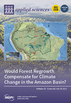
Following potential reforestation in the Amazon Basin, changes in the biophysical characteristics of the land surface may affect the fluxes of heat and moisture behavior. This study examines the impacts of potential tropical reforestation on surface energy and moisture budgets. It examines the impact of potential forest rehabilitation on atmospheric behavior using WRF.V3.9. By reforestation, the mean monthly LH also increased as much as 50 W m−2 in August in certain areas, while available moisture to the atmosphere increased by 27%, indicating possible causal mechanisms between increased LH and precipitation and emphasizing the mechanisms that were identified between the onset of the wet season and forest cover. Therefore, it is likely that forest regrowth across the basin leads to, if not reverses regional climate change, at least slowing down the rate of changes in the climate. View this paper
  • Issues are regarded as officially published after their release is announced to the table of contents alert mailing list.
  • You may sign up for e-mail alerts to receive table of contents of newly released issues.
  • PDF is the official format for papers published in both, html and pdf forms. To view the papers in pdf format, click on the "PDF Full-text" link, and use the free Adobe Reader to open them.
Order results
Result details
Section
Select all
Export citation of selected articles as:
55 pages, 5178 KiB  
Review
There Is Not Only Cupressus sempervirens L.: A Review on the Phytochemistry and Bioactivities of the Other Cupressus L. Species
by Claudio Frezza, Daniela De Vita, Fabio Sciubba, Chiara Toniolo, Lamberto Tomassini, Marcello Nicoletti, Marco Franceschin, Marcella Guiso, Armandodoriano Bianco, Mauro Serafini and Sebastiano Foddai
Appl. Sci. 2022, 12(14), 7353; https://doi.org/10.3390/app12147353 - 21 Jul 2022
Cited by 10 | Viewed by 3573
Abstract
This review article reports for the first time phytochemistry, ethnobotanical uses and pharmacological activities of all Cupressus L. species other than Cupressus sempervirens L. Indeed, the literature survey showed how many other Cupressus species are rich of important phytochemical compounds, widely used in [...] Read more.
This review article reports for the first time phytochemistry, ethnobotanical uses and pharmacological activities of all Cupressus L. species other than Cupressus sempervirens L. Indeed, the literature survey showed how many other Cupressus species are rich of important phytochemical compounds, widely used in the ethnobotanical field for several purposes and endowed with interesting biological activities, even if they are somehow neglected by the scientific community. This review aims to continue the study of these other Cupressus species and promote more research on them. Full article
(This article belongs to the Special Issue Plants: From Farm to Food and Biomedical Applications)
Show Figures

Figure 1

Figure 1
<p>Particulars of the morphological features of <span class="html-italic">Cupressus</span> species.</p>
Full article ">
11 pages, 1742 KiB  
Article
Influences of Breathing Exercises and Breathing Exercise Combined with Aerobic Exercise on Changes in Basic Spirometry Parameters in Patients with Bronchial Asthma
by Ľuboš Grznár, Dávid Sucháň, Jana Labudová, Lukáš Odráška and Ivan Matúš
Appl. Sci. 2022, 12(14), 7352; https://doi.org/10.3390/app12147352 - 21 Jul 2022
Cited by 1 | Viewed by 3219
Abstract
Scientific evidence shows that breathing or aerobic programs can improve the quality of life of asthma patients. The aim of this work was to find out the influences of breathing exercises and breathing exercises combined with aerobic exercise on changes in spirometry parameters [...] Read more.
Scientific evidence shows that breathing or aerobic programs can improve the quality of life of asthma patients. The aim of this work was to find out the influences of breathing exercises and breathing exercises combined with aerobic exercise on changes in spirometry parameters in patients with bronchial asthma. Participants: The group consisted of 33 women with bronchial asthma—mild to moderate persistent levels of FEV1 reduction (80–50%)—with a mean age of 34.73 ± 1.53 years. They were randomly assigned to experimental group 1 (EX1), experimental group 2 (EX2) or the control group (CG). Materials and methods: Changes in spirometry parameters were evaluated over a 16-week period in the three groups: CG (placebo), EX1 (breathing exercises) and EX 2 (combination of breathing exercises with an aerobic program). To evaluate the pre-training and post-training diagnostics, we used MIR Spirobank II. The influences of the experimental and control factors were assessed using the following dependent variables: forced vital capacity (FVC), forced expiratory volume in one second (FEV1), Tiffeneau–Pinelli index (FEV1/FVC ratio), peak expiratory flow (PEF) and forced mid-expiratory flow (FEF25–75%). We used the Wilcoxon t-test and the Kruskal–Wallis test to evaluate the differences in the measured parameters. To examine the effect of our protocols, we used effect size (ES). Results: In CG we observed improvements in: FVC—(5%; p < 0.05; ES = 0.437). FEV1—(7.33%; p < 0.01; ES = 0.585). FEV1/FVC ratio (5.27%; p < 0.01; ES = 0.570). PEF (11.22%; p < 0.01; ES = 0.448). FEF25–75% (7.02%; p < 0.01; ES = 0.628). In EX1 we observed improvements in: FVC (5.23%; p < 0.01; ES = 0.631), FEV1 (20.67%; p < 0.01; ES = 0.627), FEV1/FVC ratio (16.06%; p < 0.01; ES = 0.628), PEF (13.35%; p < 0.01; ES = 0.627) and FEF25–75% (13.75%; p < 0.01; ES = 0.607). In EX2 we observed improvements in: FVC (9.12%; p < 0.01; ES = 0.627), FEV1 (27.37%; p < 0.01; ES = 0.626), FEV1/FVC ratio (15.32%; p < 0.01; ES = 0.610), PEF (30.66%; p < 0.01; ES = 0.626) and FEF25–75% (58.99%; p < 0.01; ES = 0.626). Significant differences compared to the control group were observed in EX1 for FEV1 (p < 0.05) and FEV1/FVC ratio (p < 0.01); and in EX2 for FEV1 (p < 0.05), FEV1/FVC ratio (p < 0.01), PEF (p < 0.05) and FEF (p < 0.05). A significant difference between EX1 and EX2 was observed in PEF (p < 0.05). Conclusions: It appears to be that combination of breathing exercises with aerobic activities is a more beneficial option for patients with bronchial asthma. Full article
Show Figures

Figure 1

Figure 1
<p>Force vital capacity.</p>
Full article ">Figure 2
<p>Volume expired in the first second of the test.</p>
Full article ">Figure 3
<p>Tiffeneau–Pinelli index.</p>
Full article ">Figure 4
<p>Peak expiratory flow.</p>
Full article ">Figure 5
<p>Average flow between 25% and 75% of the FVC.</p>
Full article ">
17 pages, 4504 KiB  
Article
Research on Interface Slip Characteristics of Heritage Composite Timber Columns under Inclined Deformation
by Peng Chang, Qiuge Feng, Nannan Wu and Na Yang
Appl. Sci. 2022, 12(14), 7351; https://doi.org/10.3390/app12147351 - 21 Jul 2022
Viewed by 1492
Abstract
In order to study the mechanical performance and friction slip mechanism of the interface of a composite timber column under inclined deformation, the unilateral contact mechanical model of an ancient composite timber column under inclined deformation is proposed in this paper. According to [...] Read more.
In order to study the mechanical performance and friction slip mechanism of the interface of a composite timber column under inclined deformation, the unilateral contact mechanical model of an ancient composite timber column under inclined deformation is proposed in this paper. According to the limit of the inclination angle of slip point and the limit of the inclination angle of slip surface, the failure modes of the combination’s interface can be divided into three stages: the fully sticky stage, the partially sticky stage and the sliding stage. The theoretical results of the sliding displacement and shear stiffness of the combination’s interface under the effect of iron hoops were obtained by using the elastic mechanics method. Based on the shear sliding test of a composite timber column’s interface under the effect of iron hoops, the influences of different parameters on the shear sliding performance of the combination’s interface were investigated. The test results show that the number and the spacing of the iron hoops and the inclination angle of the interface are important factors affecting the shear strength of the combination’s interface. The shear strength of the interface increased with the increase in the number of iron hoops and the inclination angle of the interface. Since hoop spacing that is too large or too small cannot effectively improve the shear capacity of the interface, there is an optimal value for the hoop spacing. Full article
(This article belongs to the Special Issue Design and Assessment of Timber Structures)
Show Figures

Figure 1

Figure 1
<p>Schematic diagrams of the composite column. (<b>a</b>) The composite column in Yingzaofashi; (<b>b</b>) garlic petal column of Baoguo Temple in Ningbo; (<b>c</b>) Tibetan polyprism.</p>
Full article ">Figure 2
<p>Inclined composite timber column. (<b>a</b>) Schematic diagram of tilting; (<b>b</b>) diagram of force analysis, where <span class="html-italic">P</span> (<span class="html-italic">y</span>, <span class="html-italic">x</span>) is any point in the composite timber column.</p>
Full article ">Figure 3
<p>Stress distribution on any inclined section.</p>
Full article ">Figure 4
<p>The normal force on the interface.</p>
Full article ">Figure 5
<p>The force exerted on any micro-element.</p>
Full article ">Figure 6
<p>Specimen structure, unit: mm. (<b>a</b>) Non inclined specimen; (<b>b</b>) inclined specimen. Where Δ represents the chamfering height of the side block; <span class="html-italic">l</span> represents the initial distance between the top of the middle block and the top of the side block, which was taken as 20 mm in this test; <span class="html-italic">h</span> represents the distance between iron hoops.</p>
Full article ">Figure 7
<p>Material used for specimen. (<b>a</b>) Wood used for the composite timber column; (<b>b</b>) Q235 steel used for the iron hoop.</p>
Full article ">Figure 8
<p>Schematic diagram of the test. (<b>a</b>) Test loading setup; (<b>b</b>) the arrangement of strain gauges on the iron hoop, unit: mm.</p>
Full article ">Figure 9
<p>Shear stress–displacement curves of test groups with different numbers of iron hoops. (<b>a</b>) G1-1; (<b>b</b>) G1-2; (<b>c</b>) G1-3; (<b>d</b>) G1-4.</p>
Full article ">Figure 10
<p>Test errors. (<b>a</b>) Initial gaps between the interface surfaces; (<b>b</b>) initial shrinkage cracks and knots in the wood; (<b>c</b>) inclined iron hoop at end of loading.</p>
Full article ">Figure 11
<p>Shear stress–displacement curves of different test groups. (<b>a</b>) The number of iron hoops; (<b>b</b>) the spacing of iron hoops; (<b>c</b>) the inclination angle of the interface.</p>
Full article ">Figure 12
<p>Fitting curves of shear strength. (<b>a</b>) The number of iron hoops; (<b>b</b>) the inclination angle of the interface.</p>
Full article ">
16 pages, 5895 KiB  
Article
Parallel Accelerated Fifth-Order WENO Scheme-Based Pipeline Transient Flow Solution Model
by Tiexiang Mo and Guodong Li
Appl. Sci. 2022, 12(14), 7350; https://doi.org/10.3390/app12147350 - 21 Jul 2022
Cited by 1 | Viewed by 1515
Abstract
The water hammer phenomenon is the main problem in long-distance pipeline networks. The MOC (Method of characteristics) and finite difference methods lead to severe constraints on the mesh and Courant number, while the finite volume method of the second-order Godunov scheme has limited [...] Read more.
The water hammer phenomenon is the main problem in long-distance pipeline networks. The MOC (Method of characteristics) and finite difference methods lead to severe constraints on the mesh and Courant number, while the finite volume method of the second-order Godunov scheme has limited intermittent capture capability. These methods will produce severe numerical dissipation, affecting the computational efficiency at low Courant numbers. Based on the lax-Friedrichs flux splitting method, combined with the upstream and downstream virtual grid boundary conditions, this paper uses the high-precision fifth-order WENO scheme to reconstruct the interface flux and establishes a finite volume numerical model for solving the transient flow in the pipeline. The model adopts the GPU parallel acceleration technology to improve the program’s computational efficiency. The results show that the model maintains the excellent performance of intermittent excitation capture without spurious oscillations even at a low Courant number. Simultaneously, the model has a high degree of flexibility in meshing due to the high insensitivity to the Courant number. The number of grids in the model can be significantly reduced and higher computational efficiency can be obtained compared with MOC and the second-order Godunov scheme. Furthermore, this paper analyzes the acceleration effect in different grids. Accordingly, the acceleration effect of the GPU technique increases significantly with the increase in the number of computational grids. This model can support efficient and accurate fast simulation and prediction of non-constant transient processes in long-distance water pipeline systems. Full article
(This article belongs to the Special Issue Applied Hydrodynamics)
Show Figures

Figure 1

Figure 1
<p>Schematic diagram of pipeline meshing.</p>
Full article ">Figure 2
<p>Computational stencils of WENO.</p>
Full article ">Figure 3
<p>Bifurcated pipe interface mesh division diagram.</p>
Full article ">Figure 4
<p>GPU acceleration flowchart.</p>
Full article ">Figure 5
<p>Comparison of results of different schemes for Cr = 0.1. (<b>a</b>) Comparison of pressure wave curve at value. (<b>b</b>) Comparison of pressure wave curves at 540 m.</p>
Full article ">Figure 6
<p>Comparison of results of different schemes for Cr = 0.01. (<b>a</b>) Comparison of pressure wave curve at value. (<b>b</b>) Comparison of pressure wave curves at 10 km.</p>
Full article ">Figure 7
<p>Schematic diagram of the long-distance water pipeline.</p>
Full article ">Figure 8
<p>Results of different simulation methods. (<b>a</b>) Comparison of accuracy of different methods. (<b>b</b>) Precision comparison of GPU acceleration methods.</p>
Full article ">Figure 9
<p>The flow and water hammer wave variations at different locations when the end valves C and D are closed. (<b>a</b>) The water hammer changes with time at different positions. (<b>b</b>) Flow at different locations varies with time.</p>
Full article ">Figure 10
<p>The flow and pressure head variations at different locations when the valve is closed only at C. (<b>a</b>) The water hammer changes with time at different positions. (<b>b</b>) Flow at different locations varies with time.</p>
Full article ">Figure 11
<p>Comparison of calculation speed of different simulation methods.</p>
Full article ">Figure 12
<p>Accelerated rendering with different threads and grid numbers in GPU.</p>
Full article ">
14 pages, 10285 KiB  
Review
Fast Variable-Temperature Cryogenic Blackbody Sources for Calibration of THz Superconducting Receivers
by Mikhail Tarasov, Aleksandra Gunbina, Artem Chekushkin, Mikhail Strelkov and Valerian Edelman
Appl. Sci. 2022, 12(14), 7349; https://doi.org/10.3390/app12147349 - 21 Jul 2022
Cited by 2 | Viewed by 1847
Abstract
An electrically heated blackbody radiation source comprising thin metal film on a dielectric substrate and an integrating cavity was designed, fabricated, and experimentally studied at frequencies from 75 to 500 GHz. Analytical and numerical modeling were performed to optimize the emissivity, spectral uniformity, [...] Read more.
An electrically heated blackbody radiation source comprising thin metal film on a dielectric substrate and an integrating cavity was designed, fabricated, and experimentally studied at frequencies from 75 to 500 GHz. Analytical and numerical modeling were performed to optimize the emissivity, spectral uniformity, and modulation frequency of the radiation source with the spherical integrating cavity and thin film absorber. The blackbody emissivity (absorptivity) increased from 0.3 to 0.5 for the bare thin film on dielectric substrate, and up to 0.95 when it was placed inside the integrating cavity. The fabricated source mounted at the 0.5 K stage was used to measure the response time of a few microseconds and for sensitivity measurement down to 10−18 W/Hz1/2 of the superconductor–insulator–normal metal–insulator–superconductor (SINIS) detector at 100 mK. Full article
(This article belongs to the Special Issue Applied Superconducting Electronics)
Show Figures

Figure 1

Figure 1
<p>Methods of modeling absorption coefficient: (<b>a</b>) schematic image of modeled project (cross-section); (<b>b</b>) results of modeling for film with resistance of 550 Ω/□ on 340 μm sapphire substrate and comparison with calculation of same film from [<a href="#B6-applsci-12-07349" class="html-bibr">6</a>] (Reprinted with permission. Copyright 2021 Lemzyakov, S.A.).</p>
Full article ">Figure 2
<p>Modeled absorption coefficient for films with different resistance values (Ω/□): (<b>a</b>) irradiation from film side; (<b>b</b>) irradiation from substrate side.</p>
Full article ">Figure 3
<p>Modeled absorption coefficient of film with resistance of 188 Ω/□ on different substrates: (<b>a</b>) sapphire, silicon and quartz 340 μm substrates, irradiation of film side (<b>left</b>) and substrate side (<b>right</b>); (<b>b</b>) quartz 340 μm substrate with antireflection coating made of 65 μm-thick Teflon, irradiation from film side (<b>left</b>) and substrate side (<b>right</b>); (<b>c</b>) comparison of results of modeling absorption coefficient of thin film on quartz substrate without and with antireflection coating and with additional backshort behind antireflection coating.</p>
Full article ">Figure 4
<p>Dependence of skin depth on frequency for film with resistance of 180 Ω/□.</p>
Full article ">Figure 5
<p>Calculated absorption coefficient of films with different thickness. Irradiation from (<b>a</b>) film side and (<b>b</b>) substrate side.</p>
Full article ">Figure 6
<p>(<b>a</b>) Room-temperature demonstration model of rotating cryogenic absorber and reflector and (<b>b</b>) measured voltage response of SINIS detector to switching of aperture from reflector to thin film 10 dB absorber made on Kapton.</p>
Full article ">Figure 7
<p>Construction of integrating cavity (reprinted with permission from ref. [<a href="#B10-applsci-12-07349" class="html-bibr">10</a>], <a href="#applsci-12-07349-f004" class="html-fig">Figure 4</a>, Copyright 1978 The Optical Society): (1) Winston concentrator determining throughput AΩ; (2) second concentrator; (3) bandpass filter; (4) third cone; (5) directly irradiating bolometer in third cavity.</p>
Full article ">Figure 8
<p>(<b>a</b>) Schematic view of matching horn device (1) with integrating cavity (2) of Planck space observatory surveyor satellite and (3) incoming radiation, and (<b>b</b>) our construction of back-to-back horn (4) and flat backshort (7) with array of annular planar antennas (6) with SINIS detectors on silicon substrate (5) (Reprinted with permission from Ref. [<a href="#B11-applsci-12-07349" class="html-bibr">11</a>]. Copyright 2020 Pleiades Publishing, Ltd.).</p>
Full article ">Figure 9
<p>(<b>a</b>) Integrating cavity with NiCr film on sapphire substrate at 2.8 K stage in cryostat with the sample (left) at 280 mK stage; (<b>b</b>) photo of spherical integrating cavity for measurements with P2-69 SWR meter.</p>
Full article ">Figure 10
<p>Images of rough silicon substrate with deposited NiCr 280 nm film.</p>
Full article ">Figure 11
<p>Calculated dependence of film characteristics on surface roughness: (<b>a</b>) dependence of effective conductivity on frequency for film with roughness of 2.5 μm; (<b>b</b>) absorbance coefficient of thin film at different frequencies depending on value of effective conductivity.</p>
Full article ">Figure 11 Cont.
<p>Calculated dependence of film characteristics on surface roughness: (<b>a</b>) dependence of effective conductivity on frequency for film with roughness of 2.5 μm; (<b>b</b>) absorbance coefficient of thin film at different frequencies depending on value of effective conductivity.</p>
Full article ">Figure 12
<p>Calculation of changing temperature (T, red curves) and radiation power (P<sub>rad</sub>, black curves) at applied pulse of 10 μs (1) and 2 μs (2) and 20 and 40 V starting at t = 0. Pulse power applied to nichrome film is 0.19 and 0.75 W/cm<sup>2</sup>. Graph from [<a href="#B12-applsci-12-07349" class="html-bibr">12</a>] with permission, Copyright 2018 Pleiades Publishing, Ltd.</p>
Full article ">Figure 13
<p>Output signal (solid line) dependence on time for voltage applied to optocoupler (dot) through 14 kΩ resistor. Dashed line indicates exponent with τ = 1.8 μs, see also [<a href="#B12-applsci-12-07349" class="html-bibr">12</a>] (Reprinted with permission, Copyright 2018 Pleiades Publishing, Ltd.).</p>
Full article ">Figure 14
<p>Solid line indicates detector response to source radiation when 7 V pulse was applied for 5 ms. Dashed line indicates calculated radiation power, Reprinted with permission from Ref. [<a href="#B12-applsci-12-07349" class="html-bibr">12</a>], Copyright 2018 Pleiades Publishing, Ltd.</p>
Full article ">Figure 15
<p>Detector response to pulses applied to BB source: (<b>a</b>) U<sub>rad</sub> = 26 V, 10 μs; (<b>b</b>) U<sub>rad</sub> = 40 V 2 μs. Curve 1: measured detector response. Curve 2: calculated response taking into account dependencies of P<sub>rad</sub>(t) and registration time τ = 1.8 μs with τ<sub>det</sub> = 0. Curve 3: calculation taking into account detector response time τ<sub>det</sub> = 1.8 μs (<b>a</b>) and τ<sub>det</sub> = 0.8 μs (<b>b</b>), see also [<a href="#B12-applsci-12-07349" class="html-bibr">12</a>] (Reprinted with permission, Copyright 2018 Pleiades Publishing, Ltd.).</p>
Full article ">Figure 16
<p>Detector response for pulse amplitude U<sub>rad</sub> = 90 V, duration 0.4 μs, applied to BB radiator.</p>
Full article ">
18 pages, 6376 KiB  
Article
Crushing Analysis and Optimization of Adjacent Variable Thickness Hexagonal Tubes
by Kai Xu, Ping Xu, Jie Xing, Shuguang Yao and Qi Huang
Appl. Sci. 2022, 12(14), 7348; https://doi.org/10.3390/app12147348 - 21 Jul 2022
Viewed by 1517
Abstract
In this study, we proposed a new adjacent variable thickness hexagonal tube (AVTHT) and performed crushing analysis and crashworthiness optimization under multiple loadings. First, the finite element models were constructed and validated by experiments with four configurations of AVTHTs. Then, the numerical simulations [...] Read more.
In this study, we proposed a new adjacent variable thickness hexagonal tube (AVTHT) and performed crushing analysis and crashworthiness optimization under multiple loadings. First, the finite element models were constructed and validated by experiments with four configurations of AVTHTs. Then, the numerical simulations under axial loading and multiple oblique loadings indicated that AVTHTs under various loading angles (0°, 10°, 20°, and 30°) and three patterns (α, β, and θ) exhibited different deformation modes, force-displacement characteristics, and crashworthiness indices. This suggested that we could change and determine the plate thickness configuration to make the AVTHTs exhibit the expected crushing performance under multiple loadings. Therefore, multi-objective optimization for minimizing maximum crushing force with multiple loadings (Fmaxw) and maximizing specific energy absorption with multiple loadings (SEAw) by changing the thickness configuration under multiple loadings was conducted. The results determined the thickness design domains and indicated that certain thickness ranges should be avoided, such as the ranges of 1.55t11.6 and 1.85t11.95, which was helpful for getting AVTHTs to achieve excellent crushing performance in railway vehicles. In the pareto results, increasing t1 would not always increase the Fmaxw and SEAw. For example, when 1.75t11.8, increasing t1 would lead to decline of Fmaxw and SEAw. Full article
(This article belongs to the Section Mechanical Engineering)
Show Figures

Figure 1

Figure 1
<p>Location and geometrical details of the AVTHTs: (<b>a</b>) the installation location; (<b>b</b>) specimens; (<b>c</b>) the plate thickness configuration; (<b>d</b>) cross section; (<b>e</b>) thickness configuration of cross section.</p>
Full article ">Figure 2
<p>The compression for AVTHTs with various loading patterns: (<b>a</b>) axial loading; (<b>b</b>) along a side with thinner plate; (<b>c</b>) along a side with thicker plate; (<b>d</b>) along a corner.</p>
Full article ">Figure 3
<p>Stress-plastic strain curves.</p>
Full article ">Figure 4
<p>An experiment with a specimen tube.</p>
Full article ">Figure 5
<p>The optimization process.</p>
Full article ">Figure 6
<p>The results of the deformation process for simulations and experiments: (<b>a</b>) S2020; (<b>b</b>) S1822; (<b>c</b>) S1624; (<b>d</b>) S1426.</p>
Full article ">Figure 7
<p>Energy absorbing curves for simulations and experiments: (<b>a</b>) S2020; (<b>b</b>) S1822; (<b>c</b>) S1624; (<b>d</b>) S1426.</p>
Full article ">Figure 8
<p>The simulation results of deformation modes for seven tubes: (<b>a</b>) S2020; (<b>b</b>) S1921; (<b>c</b>) S1822; (<b>d</b>) S1723; (<b>e</b>) S1624; (<b>f</b>) S1525; (<b>g</b>) S1424; (<b>h</b>) Folds.</p>
Full article ">Figure 9
<p>Comparison of the force-displacement curves of the AVTHTs under axial loading.</p>
Full article ">Figure 10
<p>Deformation modes of the AVTHTs under different under oblique loading.</p>
Full article ">Figure 11
<p>Comparison of the force-displacement curves of the AVTHTs under different under oblique loading: (<b>a</b>) <math display="inline"><semantics> <mrow> <mi>α</mi> <mo>=</mo> <mn>10</mn> <mo>°</mo> </mrow> </semantics></math>; (<b>b</b>) <math display="inline"><semantics> <mrow> <mi>β</mi> <mo>=</mo> <mn>10</mn> <mo>°</mo> </mrow> </semantics></math>; (<b>c</b>) <math display="inline"><semantics> <mrow> <mi>θ</mi> <mo>=</mo> <mn>10</mn> <mo>°</mo> </mrow> </semantics></math>; (<b>d</b>) <math display="inline"><semantics> <mrow> <mi>α</mi> <mo>=</mo> <mn>20</mn> <mo>°</mo> </mrow> </semantics></math>; (<b>e</b>) <math display="inline"><semantics> <mrow> <mi>β</mi> <mo>=</mo> <mn>20</mn> <mo>°</mo> </mrow> </semantics></math>; (<b>f</b>) <math display="inline"><semantics> <mrow> <mi>θ</mi> <mo>=</mo> <mn>20</mn> <mo>°</mo> </mrow> </semantics></math>; (<b>g</b>) <math display="inline"><semantics> <mrow> <mi>α</mi> <mo>=</mo> <mn>30</mn> <mo>°</mo> </mrow> </semantics></math>; (<b>h</b>) <math display="inline"><semantics> <mrow> <mi>β</mi> <mo>=</mo> <mn>30</mn> <mo>°</mo> </mrow> </semantics></math>; (<b>i</b>) <math display="inline"><semantics> <mrow> <mi>θ</mi> <mo>=</mo> <mn>30</mn> <mo>°</mo> </mrow> </semantics></math>.</p>
Full article ">Figure 12
<p>Comparison of the Crashworthiness Indices of the AVTHTs under different under oblique loading: (<b>a</b>) F<sub>max</sub>; (<b>b</b>) SEA; (<b>c</b>) CFE.</p>
Full article ">Figure 12 Cont.
<p>Comparison of the Crashworthiness Indices of the AVTHTs under different under oblique loading: (<b>a</b>) F<sub>max</sub>; (<b>b</b>) SEA; (<b>c</b>) CFE.</p>
Full article ">Figure 13
<p>Pareto fronts of optimization results: (<b>a</b>) F<sub>maxw</sub> vs. −SEA<sub>w</sub>; (<b>b</b>) F<sub>maxw</sub> vs. <span class="html-italic">t1</span>; (<b>c</b>) SEA<sub>w</sub> vs. <span class="html-italic">t1</span>.</p>
Full article ">
14 pages, 3083 KiB  
Article
Evaluation of Biobed Bio-Mixture from Olive Oil Mill Wastewater Treatment as a Soil Organic Amendment in a Circular Economy Context
by Vasiliki Kinigopoulou, Evangelos Hatzigiannakis, Athanasios Guitonas, Efstathios K. Oikonomou, Stefanos Stefanou and Dionisios Gasparatos
Appl. Sci. 2022, 12(14), 7347; https://doi.org/10.3390/app12147347 - 21 Jul 2022
Cited by 3 | Viewed by 1852
Abstract
This study, based on circular economy principles and sustainable development practices, aims to present the results of soil samples analysis after their mixture with a biobed bio-mixture of straw, soil and compost, used for two consecutive years as organic bio-filter of olive oil [...] Read more.
This study, based on circular economy principles and sustainable development practices, aims to present the results of soil samples analysis after their mixture with a biobed bio-mixture of straw, soil and compost, used for two consecutive years as organic bio-filter of olive oil mill wastewater. So far, exhausted bio-mixtures used in biobeds to minimize pesticide point-source contamination turned out to contain residues of pesticides, and they are considered hazardous wastes; thus, they require special treatment before their disposal. Contrariwise, saturated bio-mixtures from bio-bed systems utilized for olive mill wastewater (OMWW) treatment not only do not require any special treatment before their final disposal but also can be exploited as a soil amendment. To this end, the effects of the used bio-mixture application in three different proportions as a soil amendment on the physical and chemical properties of medium-texture soil were investigated. The application of water simulating a typical irrigation period during a growing season took place. Upon completion of the water application, soil samples were collected from two different depths of the columns and analyzed, and leachates collected from the columns were also analyzed. Soil texture, organic matter, calcium carbonate, electrical conductivity (EC), pH, total nitrogen, nitrates, nitrites, ammonium, available phosphorus, exchangeable potassium, sodium, calcium and magnesium, exchangeable sodium percentage (ESP), cation exchange capacity (CEC), available iron, manganese, copper, zinc and boron were monitored in the soil samples as indexes of potential soil amendment, and EC, pH, nitrates, potassium, sodium, calcium, magnesium, sodium adsorption ratio (SAR), total hardness, iron, manganese, copper, zinc and boron were monitored in the leachates as indexes of potential groundwater contamination.The study demonstrated the effective use of saturated bio-mixture as an organic soil amendment, while the impact of selected amendments on groundwater was the minimum. Full article
(This article belongs to the Special Issue Soil Fertility and Plant Nutrition for Sustainable Agriculture)
Show Figures

Figure 1

Figure 1
<p>Changes of: (<b>a</b>) pH values and (<b>b</b>) EC values in the leachates of the 10 irrigation applications of the four treatments. Each value is the mean of three replicates.</p>
Full article ">Figure 2
<p>Changes of: (<b>a</b>) NO<sub>3</sub><sup>−</sup> (mg/L) concentrations and (<b>b</b>) B (mg/L) concentrations in the leachates of the 10 irrigation applications of the four treatments. Each value is the mean of three replicates.</p>
Full article ">Figure 3
<p>Changes of: (<b>a</b>) K (mg/L) concentrations, (<b>b</b>) Na (mg/L) concentrations, (<b>c</b>) Ca (mg/L) concentrations and (<b>d</b>) Mg (mg/L) concentrations in the leachates of the 10 irrigation applications of the four treatments. Each value is the mean of three replicates.</p>
Full article ">Figure 4
<p>Changes of: (<b>a</b>) SAR values and (<b>b</b>) Total Hardness (mg CaCO<sub>3</sub> L<sup>−1</sup>) values in the leachates of the 10 irrigation applications of the four treatments. Each value is the mean of three replicates.</p>
Full article ">Figure 5
<p>Changes of: (<b>a</b>) Cu (mg L<sup>−1</sup>) concentrations, (<b>b</b>) Fe (mg L<sup>−1</sup>) concentrations, (<b>c</b>) Mn (mg L<sup>−1</sup>) concentrations and (<b>d</b>) Zn (mg L<sup>−1</sup>) concentrations in the leachates of the 10 irrigation applications of the four treatments. Each value is the mean of three replicates.</p>
Full article ">Figure 6
<p>Average N<sub>total</sub> (g kg<sup>−1</sup>), NO<sub>3</sub>-N (mg kg<sup>−1</sup>) and NH<sub>4</sub>-N (mg kg<sup>−1</sup>) concentrations and their standard deviations (SD) of samples of the four treatments at 0–20 cm and 20–40 cm depth. Each value is the mean of three replicates. Different letters above each column within the same parameter evaluated, indicate significant differences among treatments.</p>
Full article ">Figure 7
<p>Average P, K, Na and Mg (mg kg<sup>−1</sup>) concentrations and their standard deviations (SD) of samples of the four treatments at 0–20 and 20–40 cm depth. Each value is the mean of three replicates. Different letters above each column within the same parameter evaluated, indicate significant differences among treatments.</p>
Full article ">Figure 8
<p>Average B (mg kg<sup>−1</sup>), Fe (mg kg<sup>−1</sup>), Mn (mg kg<sup>−1</sup>), Zn (mg kg<sup>−1</sup>) and Cu (mg kg<sup>−1</sup>) concentrations and their standard deviations (SD) of samples of the four treatments (a) at 0–20 cm depth and (b) at 20–40 cm depth. Each value is the mean of three replicates. Different letters above each column within the same parameter evaluated, indicate significant differences.</p>
Full article ">
18 pages, 2926 KiB  
Article
A Novel Method for Fault Diagnosis of Bearings with Small and Imbalanced Data Based on Generative Adversarial Networks
by Qingbin Tong, Feiyu Lu, Ziwei Feng, Qingzhu Wan, Guoping An, Junci Cao and Tao Guo
Appl. Sci. 2022, 12(14), 7346; https://doi.org/10.3390/app12147346 - 21 Jul 2022
Cited by 14 | Viewed by 2295
Abstract
The data-driven intelligent fault diagnosis method of rolling bearings has strict requirements regarding the number and balance of fault samples. However, in practical engineering application scenarios, mechanical equipment is usually in a normal state, and small and imbalanced (S & I) fault samples [...] Read more.
The data-driven intelligent fault diagnosis method of rolling bearings has strict requirements regarding the number and balance of fault samples. However, in practical engineering application scenarios, mechanical equipment is usually in a normal state, and small and imbalanced (S & I) fault samples are common, which seriously reduces the accuracy and stability of the fault diagnosis model. To solve this problem, an auxiliary classifier generative adversarial network with spectral normalization (ACGAN-SN) is proposed in this paper. First, a generation module based on a deconvolution layer is built to generate false data from Gaussian noise. Second, to enhance the training stability of the model, the data label information is used to make label constraints on the generated fake data under the basic GAN framework. Spectral normalization constraints are imposed on the output of each layer of the neural network of the discriminator to realize the Lipschitz continuity condition so as to avoid vanishing or exploding gradients. Finally, based on the generated data and the original S & I dataset, seven kinds of bearing fault datasets are made, and the prediction results of the Bi-directional Long Short-Term Memory (BiLSTM) model is verified. The results show that the data generated by ACGAN-SN can significantly promote the performance of the fault diagnosis model under the S & I fault samples. Full article
Show Figures

Figure 1

Figure 1
<p>Typical architecture of (<b>a</b>) GAN and (<b>b</b>) the auxiliary classifier GAN.</p>
Full article ">Figure 2
<p>The framework of our proposed ACGAN-SN model for fault diagnosis with S &amp; I data.</p>
Full article ">Figure 3
<p>The structure of a LSTM cell.</p>
Full article ">Figure 4
<p>The flow chart of training and testing for the proposed framework.</p>
Full article ">Figure 5
<p>Time domain waveforms of the 10 kinds of samples in the bearing dataset.</p>
Full article ">Figure 6
<p>The discrimination loss and generation loss curve of the ACGAN-SN model.</p>
Full article ">Figure 7
<p>The discrimination loss and generation accuracy curve of the ACGAN-SN model.</p>
Full article ">Figure 8
<p>The change curve of the Wasserstein distance.</p>
Full article ">Figure 9
<p>Comparison of the frequency spectrum of the real and synthetic samples data of the bearing dataset.</p>
Full article ">Figure 10
<p>Diagnosis results with different classification models after using ACGAN-SN.</p>
Full article ">Figure 11
<p>Diagnosis results with different data augmentation approaches: (<b>a</b>) MLP-based model and (<b>b</b>) BiLSTM-based model.</p>
Full article ">Figure 12
<p>The t-SNE results of (<b>a</b>) ACGAN-SN, (<b>b</b>) ACWGAN, (<b>c</b>) ACGAN, (<b>d</b>) RandomOS, and (<b>e</b>) SMOTE.</p>
Full article ">
2 pages, 174 KiB  
Editorial
Special Issue on Materials and Technologies in Oral Research
by Morena Petrini and Stefano Gennai
Appl. Sci. 2022, 12(14), 7345; https://doi.org/10.3390/app12147345 - 21 Jul 2022
Viewed by 1099
Abstract
The introduction of novel materials and technologies in oral research has permitted the rapid evolution of dentistry, as confirmed by the increasing number of publications on this topic [...] Full article
(This article belongs to the Special Issue Materials and Technologies in Oral Research)
17 pages, 5795 KiB  
Article
Mechanical Behaviors of Existing Large-Diameter Tunnel Induced by Horseshoe-Shaped Undercrossing Twin Tunnels in Gravel
by Jianye Li, Qian Fang, Xiang Liu, Jianming Du, Gan Wang and Jun Wang
Appl. Sci. 2022, 12(14), 7344; https://doi.org/10.3390/app12147344 - 21 Jul 2022
Cited by 4 | Viewed by 1843
Abstract
This article investigates and presents a case study on the Beijing Subway Line 12 excavation beneath the existing Qinghuayuan Tunnel. The composite pre-reinforcement technique was used in conjunction with the shallow tunneling method to control the distortion of the existing large-diameter tunnel. When [...] Read more.
This article investigates and presents a case study on the Beijing Subway Line 12 excavation beneath the existing Qinghuayuan Tunnel. The composite pre-reinforcement technique was used in conjunction with the shallow tunneling method to control the distortion of the existing large-diameter tunnel. When building twin tunnels underneath, this strategy considerably decreased the impact on the existing large-diameter tunnel. To systematically study the mechanical response of the existing large-diameter tunnel, a variety of sensors was embedded in the prefabricated segments just above the new twin tunnels. During the undercrossing twin tunnels procedure, the earth pressure, tunnel crown settlement, opening width of the segment joint, and the circumferential strain of the large-diameter existing tunnel were all measured. The settlement development of the existing large-diameter tunnel was categorized under six stages: (1) sedimentation, (2) heave, (3) second sedimentation, (4) second heave, (5) third sedimentation, and (6) steady state. The joint opening of the existing large-diameter tunnel changed sharply during the new undercrossing twin tunnels. The earth pressure and concrete stress of the linings rapidly increased during the new undercrossing twin tunnels. The majority of the reinforcement and concrete stresses were compressive and far lower than the yield strength, indicating that the tunnel was in a safe working condition. Full article
(This article belongs to the Special Issue Deep Rock Mass Engineering: Excavation, Monitoring, and Control)
Show Figures

Figure 1

Figure 1
<p>Views of Jing-Zhang High-speed Railway, Qinghuayuan Tunnel, and Subway Line 12.</p>
Full article ">Figure 2
<p>Diagram of existing and new tunnels (unit: m).</p>
Full article ">Figure 3
<p>Cross-section of the new tunnel (unit: mm).</p>
Full article ">Figure 4
<p>Typical intersection zone soil profile (unit: m).</p>
Full article ">Figure 5
<p>Diagram of composite pre-support with overrun pipe shed and deep hole grouting.</p>
Full article ">Figure 6
<p>(<b>a</b>) Plane layout of the monitoring section along the existing large-diameter tunnel and (<b>b</b>) layout of the monitoring points.</p>
Full article ">Figure 6 Cont.
<p>(<b>a</b>) Plane layout of the monitoring section along the existing large-diameter tunnel and (<b>b</b>) layout of the monitoring points.</p>
Full article ">Figure 7
<p>Schematic layout of component measurement points.</p>
Full article ">Figure 8
<p>The on-site installation and layout. (<b>a</b>) Diagram of reinforcement gauge installation. (<b>b</b>) Installation diagram of the earth pressure box. (<b>c</b>) Fiber optic cable box. (<b>d</b>) Appearance of part.</p>
Full article ">Figure 9
<p>Subsidence evolution of the existing large-diameter tunnel during the undercrossing twin tunnels.</p>
Full article ">Figure 10
<p>Subsidence profiles of the existing large-diameter shield tunnel.</p>
Full article ">Figure 11
<p>Induced hoop stress of the existing tunnel in the transverse section. (<b>a</b>) Far-field excavation; (<b>b</b>) Forepoling reinforcement; (<b>c</b>) Right line underpass construction; (<b>d</b>) Deep hole grouting in the left line and post-wall grouting in the right line; (<b>e</b>) Left line under crossing construction; (<b>f</b>) Grouting and stabilization behind the left line wall.</p>
Full article ">Figure 11 Cont.
<p>Induced hoop stress of the existing tunnel in the transverse section. (<b>a</b>) Far-field excavation; (<b>b</b>) Forepoling reinforcement; (<b>c</b>) Right line underpass construction; (<b>d</b>) Deep hole grouting in the left line and post-wall grouting in the right line; (<b>e</b>) Left line under crossing construction; (<b>f</b>) Grouting and stabilization behind the left line wall.</p>
Full article ">Figure 12
<p>The opening width of the segment joint versus time at CS12.</p>
Full article ">Figure 13
<p>The opening width of the segment joint versus time at CS6.</p>
Full article ">Figure 14
<p>Measured and fitted settlement profiles.</p>
Full article ">Figure 15
<p>Earth pressure evolution and mechanical responses of the existing large-diameter tunnel: (<b>a</b>) earth pressure and (<b>b</b>) reinforcement stress.</p>
Full article ">
10 pages, 278 KiB  
Article
Physical Development Differences between Professional Soccer Players from Different Competitive Levels
by Cíntia França, Andreas Ihle, Adilson Marques, Hugo Sarmento, Francisco Martins, Ricardo Henriques and Élvio Rúbio Gouveia
Appl. Sci. 2022, 12(14), 7343; https://doi.org/10.3390/app12147343 - 21 Jul 2022
Cited by 6 | Viewed by 2560
Abstract
In soccer, physical development is crucial for developing optimal performance. This study aimed to assess and compare the physical development of elite and non-elite professional soccer players. Seventy-eight male professional football players divided into four competitive levels participated in this study: the elite [...] Read more.
In soccer, physical development is crucial for developing optimal performance. This study aimed to assess and compare the physical development of elite and non-elite professional soccer players. Seventy-eight male professional football players divided into four competitive levels participated in this study: the elite group (EG), the non-elite group A (NEG-A), the non-elite group B (NEG-B), and the under 23 group (U23). Body composition, static strength, lower-body explosive strength, flexibility, and balance were assessed. No significant statistical differences between elite and non-elite players were seen in body composition parameters. However, the EG performed better in static strength, lower-body explosive strength, flexibility, and balance, even after adjusting for the effects of chronological age. The analysis showed that the competitive level (group) explained 25% to 29% of the variance observed in the lower-body explosive strength tasks. Sports staff and coaches in different age categories or competitive levels should include specific lower-body explosive strength content during soccer training to promote players’ long-term development towards the elite level. Full article
(This article belongs to the Special Issue New Trends in Fitness and Sports Performance Analysis)
11 pages, 28404 KiB  
Article
Development of a Novel Gear-like Disk Resonator Applied in Gyroscope
by Liutao Gu, Weiping Zhang, Jun Feng and Zhihan Zhang
Appl. Sci. 2022, 12(14), 7342; https://doi.org/10.3390/app12147342 - 21 Jul 2022
Cited by 2 | Viewed by 1401
Abstract
This paper proposes a novel gear-like disk resonator (GDR). The design, fabrication, and characterization of GDR are presented. In comparison with a ring-like disk resonator (RDR), a GDR replaces the circular rings with meander-shaped rings consisting of linear beams. The finite element method [...] Read more.
This paper proposes a novel gear-like disk resonator (GDR). The design, fabrication, and characterization of GDR are presented. In comparison with a ring-like disk resonator (RDR), a GDR replaces the circular rings with meander-shaped rings consisting of linear beams. The finite element method (FEM) is implemented, and the simulation results show that the GDR has a much lower frequency and effective stiffness, higher quality factor (Q), and better immunity to crystal orientation error. Affected by high Q and small frequency splits, the mechanical sensitivity (Smech) is shown to increase greatly. GDR and RDR with the same structure parameters are built side-by-side on the same wafer, and prototypes are fabricated through the SOI fabrication technique. The frequency response test and ring-down test are implemented using a readout circuit under a vacuum condition (5 Pa) at room temperature. The frequency split (9.1 Hz) of the GDR is about 2.8 times smaller than that (25.8 Hz) of the RDR without electrostatic tuning. Compared with the RDR, the Q (19.2 k) and decay time constant (0.59 s) of the GDR are improved by 145% and 236%, respectively. The experimental results show great promise for the GDR being used as a gear-like disk resonator gyroscope (GDRG). Full article
Show Figures

Figure 1

Figure 1
<p>Design strategy: (<b>a</b>) the structure of GDR; (<b>b</b>) the working mode of GDR.</p>
Full article ">Figure 2
<p>The equivalent constraint in COMSOL Multiphysics.</p>
Full article ">Figure 3
<p>Performances comparison between GDR and RDR.</p>
Full article ">Figure 4
<p>Effects of <span class="html-italic">α</span> on frequency split.</p>
Full article ">Figure 5
<p>Fabrication process flow of GDR and RDR.</p>
Full article ">Figure 6
<p>SEM images of fabricated GDR and RDR: (<b>a</b>) overview of GDR; (<b>b</b>) overview of RDR; (<b>c</b>) detailed view of GDR; (<b>d</b>) detailed view of RDR.</p>
Full article ">Figure 7
<p>Experimental setup for frequency response test and ring-down test.</p>
Full article ">Figure 8
<p>Experiment results of frequency response and ring-down test: (<b>a</b>) GDR. (<b>b</b>) RDR.</p>
Full article ">
17 pages, 5181 KiB  
Article
Screening Additives for Amending Compacted Clay Covers to Enhance Diffusion Barrier Properties and Moisture Retention Performance
by Min Wang, Jiaming Wen, Heng Zhuang, Weiyi Xia, Ningjun Jiang and Yanjun Du
Appl. Sci. 2022, 12(14), 7341; https://doi.org/10.3390/app12147341 - 21 Jul 2022
Cited by 4 | Viewed by 1592
Abstract
The cover systems in contaminated sites have some problems, including desiccation cracks, which would lead to degradation of the barrier performance. This study presented a systemic laboratory experimental investigation on the liquid–plastic limit, moisture retention, hydraulic conductivity (k), and gas diffusion [...] Read more.
The cover systems in contaminated sites have some problems, including desiccation cracks, which would lead to degradation of the barrier performance. This study presented a systemic laboratory experimental investigation on the liquid–plastic limit, moisture retention, hydraulic conductivity (k), and gas diffusion barrier properties of amended compacted clay by attapulgite and diatomite for controlling desiccation cracks and migration of water and volatile organic compounds (VOCs). The results showed that the attapulgite could enhance the moisture retention and liquid limit of amended compacted clay. Diatomite could reduce the gas diffusion coefficient (Dθ) significantly. The compacted clay amended by the dual-additives component of attapulgite and diatomite could enhance the liquid limit, moisture retention percent, gas barrier property, and hydraulic performance compared with the unamended clay. Based on the experimental data obtained, the dosage of additives was targeted to be 5%. The moisture retention percent of dual-additives (attapulgite 4% and diatomite 1%) amended clay increased by 82%, the k decreased by 25%, and the Dθ decreased by 42% compared with unamended clay. Scanning electron microscopy (SEM), BET-specific surface area test method (BET), Mercury Intrusion Porosimetry (MIP), and thermogravimetric analysis (TGA) indicated the enhancement mechanism of additives-amended compacted clay. Full article
(This article belongs to the Special Issue Advances in Soil Pollution and Geotechnical Environment)
Show Figures

Figure 1

Figure 1
<p>Problems of compacted clay cover desiccation and possible migration of VOCs [<a href="#B6-applsci-12-07341" class="html-bibr">6</a>,<a href="#B7-applsci-12-07341" class="html-bibr">7</a>,<a href="#B8-applsci-12-07341" class="html-bibr">8</a>,<a href="#B9-applsci-12-07341" class="html-bibr">9</a>,<a href="#B10-applsci-12-07341" class="html-bibr">10</a>,<a href="#B11-applsci-12-07341" class="html-bibr">11</a>,<a href="#B12-applsci-12-07341" class="html-bibr">12</a>,<a href="#B13-applsci-12-07341" class="html-bibr">13</a>,<a href="#B14-applsci-12-07341" class="html-bibr">14</a>].</p>
Full article ">Figure 2
<p>Compaction curve of the clay and dual-additives-amended clay.</p>
Full article ">Figure 3
<p>The chamber of soil gas diffusion test.</p>
Full article ">Figure 4
<p>The plasticity chart of the clay amended by additives with different dosages and ratios.</p>
Full article ">Figure 5
<p>The moisture retention percent with different dosages of attapulgite and diatomite.</p>
Full article ">Figure 6
<p>The moisture retention percent with different ratios of attapulgite to diatomite.</p>
Full article ">Figure 7
<p>The gas diffusion coefficient with different dosages of attapulgite and diatomite.</p>
Full article ">Figure 8
<p>The effect of ratios of additives on the gas diffusion coefficient.</p>
Full article ">Figure 9
<p>The flexible wall penetration test results of amended compacted clay.</p>
Full article ">Figure 10
<p>SEM images of compacted clay specimens.</p>
Full article ">Figure 11
<p>MIP results of amended compacted clay specimens: (<b>a</b>) cumulative intruded pore volume vs. pore size diameter; and (<b>b</b>) incremental intruded pore volume.</p>
Full article ">Figure 12
<p>BET tests results of clay specimens amended by attapulgite, diatomite, dual-additives, and unamended.</p>
Full article ">Figure 13
<p>TG tests results of specimens: (<b>a</b>) Unamended; (<b>b</b>) Attapulgite-amended; (<b>c</b>) Diatomite-amended; and (<b>d</b>) Dual-additives-amended.</p>
Full article ">
21 pages, 9049 KiB  
Review
Seismic Analysis of Slender Monumental Structures: Current Strategies and Challenges
by Maria Giovanna Masciotta and Paulo B. Lourenço
Appl. Sci. 2022, 12(14), 7340; https://doi.org/10.3390/app12147340 - 21 Jul 2022
Cited by 13 | Viewed by 2367
Abstract
The preservation and seismic risk mitigation of built cultural heritage is considered today as a major priority in the international political agenda. Among the great variety of heritage structures spread worldwide, masonry towers belong to one of the most vulnerable categories against earthquake [...] Read more.
The preservation and seismic risk mitigation of built cultural heritage is considered today as a major priority in the international political agenda. Among the great variety of heritage structures spread worldwide, masonry towers belong to one of the most vulnerable categories against earthquake actions due to their morphological and material singularity. The proper understanding of the structural behavior of these artefacts at the micro, meso and macro scales, combined with a thorough knowledge of the best analysis practices deriving from the shared experience of the scientific community working in this field, is a fundamental prerequisite to appropriately address their seismic assessment. In this context, the present work offers an extensive discussion on the major challenges that slender monumental towers pose in terms of characterization of their actual behavior under seismic actions. A critical appraisal of the principal analysis methods applicable to the study of these structures is also presented along with a brief review of the existing modelling strategies for their numerical representation. Relevant examples are discussed in support of each argument. In spite of being a relatively young discipline, earthquake engineering has made remarkable progress in the last years and appropriate modi operandi have been consolidating to tackle the seismic assessment of unconventional systems, such as slender heritage structures. The work is conceived in a format of interest for both practitioners and researchers approaching the seismic assessment of this type of structures, and for those in need of an overall practical review of the topic. Full article
(This article belongs to the Special Issue Advanced Seismic Evaluation of Relevant Architectures)
Show Figures

Figure 1

Figure 1
<p>Examples of ancient masonry section with complex arrangements of units.</p>
Full article ">Figure 2
<p>Masonry failure mechanisms (adapted from [<a href="#B27-applsci-12-07340" class="html-bibr">27</a>]): (<b>a</b>) joint tensile cracking; (<b>b</b>) joint slipping; (<b>c</b>) unit direct tensile cracking; (<b>d</b>) unit diagonal tensile cracking; (<b>e</b>) masonry crushing.</p>
Full article ">Figure 3
<p>Experimental results on stone masonry shear walls [<a href="#B21-applsci-12-07340" class="html-bibr">21</a>]: (<b>a</b>) specimen geometries; (<b>b</b>) force−displacement diagrams; (<b>c</b>) failure mechanisms.</p>
Full article ">Figure 4
<p>Seismic response of the Church of Jerónimos Monastery, Portugal (adapted from [<a href="#B46-applsci-12-07340" class="html-bibr">46</a>,<a href="#B47-applsci-12-07340" class="html-bibr">47</a>]): (<b>a</b>) exterior view; (<b>b</b>) location of strong motion recorders (A1: chancel base; A2: nave vault extrados); (<b>c</b>,<b>d</b>) acceleration response at the base and at the top of the nave during the earthquake; (<b>e</b>) measured response spectra.</p>
Full article ">Figure 5
<p>Amplification effects during the 2016 Bagan earthquake in Myanmar.</p>
Full article ">Figure 6
<p>Experimental mode shapes of the Mogadouro clock tower—undeformed structure in yellow wireframe (reprinted with permission from Ref. [<a href="#B49-applsci-12-07340" class="html-bibr">49</a>]. Copyright 2018, Elsevier).</p>
Full article ">Figure 7
<p>Overview of the Mogadouro tower before, during and after the rehabilitation works.</p>
Full article ">Figure 8
<p>Seismic assessment of the Qutb Minar tower. Comparison of the results from different analysis methods [<a href="#B64-applsci-12-07340" class="html-bibr">64</a>]: (<b>a</b>) capacity curves for pushover analyses, (<b>b</b>) maximum load factor and displacements along the minaret height for dynamic analyses, (<b>c</b>) displacements and drifts along the minaret height for modal pushover and non-linear dynamic analyses.</p>
Full article ">Figure 9
<p>Qutb Minar tower: (<b>a</b>) exterior view and (<b>b</b>) detail of the fluted shaft.</p>
Full article ">Figure 10
<p>Modelling strategies for masonry structures (adapted from [<a href="#B27-applsci-12-07340" class="html-bibr">27</a>]): (<b>a</b>) detailed micro-modelling, (<b>b</b>) simplified micro-modelling, (<b>c</b>) macro-modelling.</p>
Full article ">Figure 11
<p>Examples of models adopted for the blind predictions of the (<b>a</b>) tested masonry structures: (<b>b</b>) models with rigid macro-blocks; (<b>c</b>) FEM models and (<b>d</b>) DEM models.</p>
Full article ">Figure 12
<p>Seismic acceleration capacity (PGA) obtained from the blind predictions [<a href="#B98-applsci-12-07340" class="html-bibr">98</a>] (green and yellow bars correspond to good and fair mechanism predictions).</p>
Full article ">Figure 13
<p>Framework of the scientific approach to the analysis of architectural heritage.</p>
Full article ">
27 pages, 9266 KiB  
Article
Empirical Perturbation Analysis of Two Adversarial Attacks: Black Box versus White Box
by Raluca Chitic, Ali Osman Topal and Franck Leprévost
Appl. Sci. 2022, 12(14), 7339; https://doi.org/10.3390/app12147339 - 21 Jul 2022
Cited by 1 | Viewed by 1606
Abstract
Through the addition of humanly imperceptible noise to an image classified as belonging to a category ca, targeted adversarial attacks can lead convolutional neural networks (CNNs) to classify a modified image as belonging to any predefined target class [...] Read more.
Through the addition of humanly imperceptible noise to an image classified as belonging to a category ca, targeted adversarial attacks can lead convolutional neural networks (CNNs) to classify a modified image as belonging to any predefined target class ctca. To achieve a better understanding of the inner workings of adversarial attacks, this study analyzes the adversarial images created by two completely opposite attacks against 10 ImageNet-trained CNNs. A total of 2×437 adversarial images are created by EAtarget,C, a black-box evolutionary algorithm (EA), and by the basic iterative method (BIM), a white-box, gradient-based attack. We inspect and compare these two sets of adversarial images from different perspectives: the behavior of CNNs at smaller image regions, the image noise frequency, the adversarial image transferability, the image texture change, and penultimate CNN layer activations. We find that texture change is a side effect rather than a means for the attacks and that ct-relevant features only build up significantly from image regions of size 56×56 onwards. In the penultimate CNN layers, both attacks increase the activation of units that are positively related to ct and units that are negatively related to ca. In contrast to EAtarget,C’s white noise nature, BIM predominantly introduces low-frequency noise. BIM affects the original ca features more than EAtarget,C, thus producing slightly more transferable adversarial images. However, the transferability with both attacks is low, since the attacks’ ct-related information is specific to the output layers of the targeted CNN. We find that the adversarial images are actually more transferable at regions with sizes of 56×56 than at full scale. Full article
(This article belongs to the Special Issue Explainable Artificial Intelligence (XAI))
Show Figures

Figure 1

Figure 1
<p>Single-patch replacement for <math display="inline"><semantics> <msubsup> <mi mathvariant="script">A</mi> <mn>5</mn> <mn>4</mn> </msubsup> </semantics></math> and <math display="inline"><semantics> <mrow> <mi mathvariant="script">C</mi> <mo>=</mo> <msub> <mi mathvariant="script">C</mi> <mn>6</mn> </msub> </mrow> </semantics></math>. The four pairs of graphs correspond to patches with sizes of <math display="inline"><semantics> <mrow> <mn>16</mn> <mo>×</mo> <mn>16</mn> </mrow> </semantics></math>, <math display="inline"><semantics> <mrow> <mn>32</mn> <mo>×</mo> <mn>32</mn> </mrow> </semantics></math>, <math display="inline"><semantics> <mrow> <mn>56</mn> <mo>×</mo> <mn>56</mn> </mrow> </semantics></math>, and <math display="inline"><semantics> <mrow> <mn>112</mn> <mo>×</mo> <mn>112</mn> </mrow> </semantics></math>. Each pair represents the step-wise plot of <math display="inline"><semantics> <mrow> <mi>l</mi> <mi>o</mi> <mi>g</mi> <mo>(</mo> <msubsup> <mi>o</mi> <mi>I</mi> <mi mathvariant="script">C</mi> </msubsup> <mrow> <mo>[</mo> <mi>a</mi> <mo>]</mo> </mrow> <mo>)</mo> </mrow> </semantics></math> (<b>left</b> graph) and of <math display="inline"><semantics> <mrow> <mi>l</mi> <mi>o</mi> <mi>g</mi> <mo>(</mo> <msubsup> <mi>o</mi> <mi>I</mi> <mi mathvariant="script">C</mi> </msubsup> <mrow> <mo>[</mo> <mi>t</mi> <mo>]</mo> </mrow> <mo>)</mo> </mrow> </semantics></math> (<b>right</b> graph) for the EA (blue curve) and BIM (orange curve). The red horizontal line recalls the <math display="inline"><semantics> <msub> <mi>c</mi> <mi>a</mi> </msub> </semantics></math>-label value (<b>left</b> graph) or the <math display="inline"><semantics> <msub> <mi>c</mi> <mi>t</mi> </msub> </semantics></math>-label value (<b>right</b> graph) of <math display="inline"><semantics> <msubsup> <mi mathvariant="script">A</mi> <mn>5</mn> <mn>4</mn> </msubsup> </semantics></math> with no replaced patch.</p>
Full article ">Figure 2
<p>Display of the noise and histogram of the perturbations added by the EA (<b>left</b> pair) and by BIM (<b>right</b> pair) to the red channel of <math display="inline"><semantics> <msubsup> <mi mathvariant="script">A</mi> <mn>5</mn> <mn>4</mn> </msubsup> </semantics></math> to fool <math display="inline"><semantics> <msub> <mi mathvariant="script">C</mi> <mn>6</mn> </msub> </semantics></math>.</p>
Full article ">Figure 3
<p>For <math display="inline"><semantics> <mrow> <mi>a</mi> <mi>t</mi> <mi>k</mi> <mo>=</mo> <mi>E</mi> <mi>A</mi> </mrow> </semantics></math> (<b>left</b> pair) and <math display="inline"><semantics> <mrow> <mi>a</mi> <mi>t</mi> <mi>k</mi> <mo>=</mo> <mi>B</mi> <mi>I</mi> <mi>M</mi> </mrow> </semantics></math> (<b>right</b> pair), representation of <math display="inline"><semantics> <mrow> <mo stretchy="false">|</mo> <mi>D</mi> <mi>F</mi> <mi>T</mi> <mo stretchy="false">(</mo> <msubsup> <mrow> <mi mathvariant="script">D</mi> </mrow> <mn>6</mn> <mrow> <mi>a</mi> <mi>t</mi> <mi>k</mi> </mrow> </msubsup> <mrow> <mo stretchy="false">(</mo> <msubsup> <mi mathvariant="script">A</mi> <mn>5</mn> <mn>4</mn> </msubsup> <mo stretchy="false">)</mo> </mrow> <mo>−</mo> <msubsup> <mi mathvariant="script">A</mi> <mn>5</mn> <mn>4</mn> </msubsup> <mo stretchy="false">)</mo> <mo stretchy="false">|</mo> </mrow> </semantics></math> (magn (diff), first image) and <math display="inline"><semantics> <mrow> <mrow> <mo stretchy="false">|</mo> <mi>D</mi> <mi>F</mi> <mi>T</mi> </mrow> <mrow> <mo stretchy="false">(</mo> <msubsup> <mrow> <mi mathvariant="script">D</mi> </mrow> <mn>6</mn> <mrow> <mi>a</mi> <mi>t</mi> <mi>k</mi> </mrow> </msubsup> <mrow> <mo stretchy="false">(</mo> <msubsup> <mi mathvariant="script">A</mi> <mn>5</mn> <mn>4</mn> </msubsup> <mo stretchy="false">)</mo> </mrow> <mo stretchy="false">)</mo> </mrow> <mrow> <mo stretchy="false">|</mo> <mo>−</mo> <mo stretchy="false">|</mo> <mi>D</mi> <mi>F</mi> <mi>T</mi> </mrow> <mrow> <mo stretchy="false">(</mo> <msubsup> <mi mathvariant="script">A</mi> <mn>5</mn> <mn>4</mn> </msubsup> <mo stretchy="false">)</mo> </mrow> <mrow> <mo stretchy="false">|</mo> </mrow> </mrow> </semantics></math> (diff (magn), second image) for the red channel.</p>
Full article ">Figure 4
<p>For <math display="inline"><semantics> <mrow> <mi>a</mi> <mi>t</mi> <mi>k</mi> <mo>=</mo> <mi>E</mi> <mi>A</mi> </mrow> </semantics></math> (<b>left</b>) and <math display="inline"><semantics> <mrow> <mi>a</mi> <mi>t</mi> <mi>k</mi> <mo>=</mo> <mi>B</mi> <mi>I</mi> <mi>M</mi> </mrow> </semantics></math> (<b>right</b>), autocorrelation of <math display="inline"><semantics> <mrow> <msubsup> <mrow> <mi mathvariant="script">D</mi> </mrow> <mn>6</mn> <mrow> <mi>a</mi> <mi>t</mi> <mi>k</mi> </mrow> </msubsup> <mrow> <mo stretchy="false">(</mo> <msubsup> <mi mathvariant="script">A</mi> <mn>5</mn> <mn>4</mn> </msubsup> <mo stretchy="false">)</mo> </mrow> <mo>−</mo> <msubsup> <mi mathvariant="script">A</mi> <mn>5</mn> <mn>4</mn> </msubsup> </mrow> </semantics></math> for the red channel.</p>
Full article ">Figure 5
<p>For <math display="inline"><semantics> <mrow> <mi>a</mi> <mi>t</mi> <mi>k</mi> <mo>=</mo> <mi>EA</mi> </mrow> </semantics></math> (first and second rows) and <math display="inline"><semantics> <mrow> <mi>a</mi> <mi>t</mi> <mi>k</mi> <mo>=</mo> <mi>B</mi> <mi>I</mi> <mi>M</mi> </mrow> </semantics></math> (third and fourth rows), the following images are fed to <math display="inline"><semantics> <msub> <mi mathvariant="script">C</mi> <mn>6</mn> </msub> </semantics></math>: <math display="inline"><semantics> <msubsup> <mi mathvariant="script">A</mi> <mn>5</mn> <mn>4</mn> </msubsup> </semantics></math> and <math display="inline"><semantics> <mrow> <msubsup> <mrow> <mi mathvariant="script">D</mi> </mrow> <mn>6</mn> <mrow> <mi>a</mi> <mi>t</mi> <mi>k</mi> </mrow> </msubsup> <mrow> <mo stretchy="false">(</mo> <msubsup> <mi mathvariant="script">A</mi> <mn>5</mn> <mn>4</mn> </msubsup> <mo stretchy="false">)</mo> </mrow> </mrow> </semantics></math> (first pair), <math display="inline"><semantics> <mrow> <mi>s</mi> <mi>h</mi> <mo stretchy="false">(</mo> <msubsup> <mi mathvariant="script">A</mi> <mn>5</mn> <mn>4</mn> </msubsup> <mo>,</mo> <mn>32</mn> <mo stretchy="false">)</mo> </mrow> </semantics></math> and <math display="inline"><semantics> <mrow> <mi>s</mi> <mi>h</mi> <mo stretchy="false">(</mo> <msubsup> <mrow> <mi mathvariant="script">D</mi> </mrow> <mn>6</mn> <mrow> <mi>a</mi> <mi>t</mi> <mi>k</mi> </mrow> </msubsup> <mrow> <mo stretchy="false">(</mo> <msubsup> <mi mathvariant="script">A</mi> <mn>5</mn> <mn>4</mn> </msubsup> <mo stretchy="false">)</mo> </mrow> <mo>,</mo> <mn>32</mn> <mo stretchy="false">)</mo> </mrow> </semantics></math> (second pair), <math display="inline"><semantics> <mrow> <mi>s</mi> <mi>h</mi> <mo stretchy="false">(</mo> <msubsup> <mi mathvariant="script">A</mi> <mn>5</mn> <mn>4</mn> </msubsup> <mo>,</mo> <mn>56</mn> <mo stretchy="false">)</mo> </mrow> </semantics></math> and <math display="inline"><semantics> <mrow> <mi>s</mi> <mi>h</mi> <mo stretchy="false">(</mo> <msubsup> <mrow> <mi mathvariant="script">D</mi> </mrow> <mn>6</mn> <mrow> <mi>a</mi> <mi>t</mi> <mi>k</mi> </mrow> </msubsup> <mrow> <mo stretchy="false">(</mo> <msubsup> <mi mathvariant="script">A</mi> <mn>5</mn> <mn>4</mn> </msubsup> <mo stretchy="false">)</mo> </mrow> <mo>,</mo> <mn>56</mn> <mo stretchy="false">)</mo> </mrow> </semantics></math> (third pair), and <math display="inline"><semantics> <mrow> <mi>s</mi> <mi>h</mi> <mo stretchy="false">(</mo> <msubsup> <mi mathvariant="script">A</mi> <mn>5</mn> <mn>4</mn> </msubsup> <mo>,</mo> <mn>112</mn> <mo stretchy="false">)</mo> </mrow> </semantics></math> and <math display="inline"><semantics> <mrow> <mi>s</mi> <mi>h</mi> <mo stretchy="false">(</mo> <msubsup> <mrow> <mi mathvariant="script">D</mi> </mrow> <mn>6</mn> <mrow> <mi>a</mi> <mi>t</mi> <mi>k</mi> </mrow> </msubsup> <mrow> <mo stretchy="false">(</mo> <msubsup> <mi mathvariant="script">A</mi> <mn>5</mn> <mn>4</mn> </msubsup> <mo stretchy="false">)</mo> </mrow> <mo>,</mo> <mn>112</mn> <mo stretchy="false">)</mo> </mrow> </semantics></math> (third pair). In each pair of graphs, the <b>left</b> graph displays the <math display="inline"><semantics> <msub> <mi>c</mi> <mi>a</mi> </msub> </semantics></math>-label values given by <math display="inline"><semantics> <msub> <mi mathvariant="script">C</mi> <mn>6</mn> </msub> </semantics></math> as the images are band-stop filtered with bandwidths centred on different <math display="inline"><semantics> <mrow> <mi>r</mi> <mi>c</mi> </mrow> </semantics></math> values, and the <b>right</b> graph displays the <math display="inline"><semantics> <msub> <mi>c</mi> <mi>t</mi> </msub> </semantics></math>-label values, <span class="html-italic">mutatis mutandis</span>.</p>
Full article ">Figure 6
<p>Heatmaps obtained with the ancestor <math display="inline"><semantics> <mrow> <mi mathvariant="script">A</mi> <mo>=</mo> <msubsup> <mi mathvariant="script">A</mi> <mrow> <mn>10</mn> </mrow> <mn>8</mn> </msubsup> </mrow> </semantics></math> and the adversarial image <math display="inline"><semantics> <mrow> <mi mathvariant="script">D</mi> <mrow> <mo stretchy="false">(</mo> <mi mathvariant="script">A</mi> <mo stretchy="false">)</mo> </mrow> <mo>=</mo> <msubsup> <mrow> <mi mathvariant="script">D</mi> </mrow> <mn>6</mn> <mrow> <mi>a</mi> <mi>t</mi> <mi>k</mi> </mrow> </msubsup> <mrow> <mo stretchy="false">(</mo> <msubsup> <mi mathvariant="script">A</mi> <mrow> <mn>10</mn> </mrow> <mn>8</mn> </msubsup> <mo stretchy="false">)</mo> </mrow> </mrow> </semantics></math> pictured in (<b>a</b>), where <math display="inline"><semantics> <mrow> <mi>a</mi> <mi>t</mi> <mi>k</mi> <mo>=</mo> </mrow> </semantics></math> EA in the 1st row and <math display="inline"><semantics> <mrow> <mi>a</mi> <mi>t</mi> <mi>k</mi> <mo>=</mo> </mrow> </semantics></math> BIM in the 2nd row. From (<b>b</b>–<b>e</b>), the heat maps are created using BagNet-17 and represent the following: 10% smallest values of <math display="inline"><semantics> <mrow> <msub> <mi>c</mi> <mi>a</mi> </msub> <mrow> <mo>(</mo> <mi>P</mi> <mrow> <mo>(</mo> <mi mathvariant="script">D</mi> <mrow> <mo>(</mo> <mi mathvariant="script">A</mi> <mo>)</mo> </mrow> <mo>)</mo> </mrow> <mo>)</mo> </mrow> <mo>−</mo> <msub> <mi>c</mi> <mi>a</mi> </msub> <mrow> <mo>(</mo> <mi>P</mi> <mrow> <mo>(</mo> <mi mathvariant="script">A</mi> <mo>)</mo> </mrow> <mo>)</mo> </mrow> </mrow> </semantics></math> (<b>b</b>); 10% largest values of <math display="inline"><semantics> <mrow> <msub> <mi>c</mi> <mi>t</mi> </msub> <mrow> <mo>(</mo> <mi>P</mi> <mrow> <mo>(</mo> <mi mathvariant="script">D</mi> <mrow> <mo>(</mo> <mi mathvariant="script">A</mi> <mo>)</mo> </mrow> <mo>)</mo> </mrow> <mo>)</mo> </mrow> <mo>−</mo> <msub> <mi>c</mi> <mi>t</mi> </msub> <mrow> <mo>(</mo> <mi>P</mi> <mrow> <mo>(</mo> <mi mathvariant="script">A</mi> <mo>)</mo> </mrow> <mo>)</mo> </mrow> </mrow> </semantics></math> (<b>c</b>); 10% largest values of <math display="inline"><semantics> <mrow> <msub> <mi>c</mi> <mi>a</mi> </msub> <mrow> <mo>(</mo> <mi>P</mi> <mrow> <mo>(</mo> <mi mathvariant="script">D</mi> <mrow> <mo>(</mo> <mi mathvariant="script">A</mi> <mo>)</mo> </mrow> <mo>)</mo> </mrow> <mo>)</mo> </mrow> <mo>−</mo> <msub> <mi>c</mi> <mi>t</mi> </msub> <mrow> <mo>(</mo> <mi>P</mi> <mrow> <mo>(</mo> <mi mathvariant="script">D</mi> <mrow> <mo>(</mo> <mi mathvariant="script">A</mi> <mo>)</mo> </mrow> <mo>)</mo> </mrow> <mo>)</mo> </mrow> </mrow> </semantics></math> (<b>d</b>); 10% largest values of <math display="inline"><semantics> <mrow> <msub> <mi>c</mi> <mi>t</mi> </msub> <mrow> <mo>(</mo> <mi>P</mi> <mrow> <mo>(</mo> <mi mathvariant="script">D</mi> <mrow> <mo>(</mo> <mi mathvariant="script">A</mi> <mo>)</mo> </mrow> <mo>)</mo> </mrow> <mo>)</mo> </mrow> <mo>−</mo> <msub> <mi>c</mi> <mi>a</mi> </msub> <mrow> <mo>(</mo> <mi>P</mi> <mrow> <mo>(</mo> <mi mathvariant="script">D</mi> <mrow> <mo>(</mo> <mi mathvariant="script">A</mi> <mo>)</mo> </mrow> <mo>)</mo> </mrow> <mo>)</mo> </mrow> </mrow> </semantics></math> (<b>e</b>). Heatmap (<b>f</b>) is obtained with <math display="inline"><semantics> <msub> <mi mathvariant="script">C</mi> <mi>k</mi> </msub> </semantics></math> and represents the 10% largest values of <math display="inline"><semantics> <mrow> <msub> <mi>c</mi> <mi>t</mi> </msub> <mrow> <mo>(</mo> <mi>I</mi> <mi>P</mi> <mrow> <mo>(</mo> <mi mathvariant="script">D</mi> <mrow> <mo>(</mo> <mi mathvariant="script">A</mi> <mo>)</mo> </mrow> <mo>)</mo> </mrow> <mo>)</mo> </mrow> <mo>−</mo> <msub> <mi>c</mi> <mi>t</mi> </msub> <mrow> <mo>(</mo> <mi mathvariant="script">A</mi> <mo>)</mo> </mrow> </mrow> </semantics></math>.</p>
Full article ">Figure 7
<p>Evolution of <math display="inline"><semantics> <mrow> <mi>l</mi> <mi>o</mi> <mi>g</mi> <mo stretchy="false">(</mo> <mi>o</mi> <mo>[</mo> <mi>a</mi> <mo>]</mo> <mo stretchy="false">)</mo> </mrow> </semantics></math>, <math display="inline"><semantics> <mrow> <mi>l</mi> <mi>o</mi> <mi>g</mi> <mo stretchy="false">(</mo> <mi>o</mi> <mo>[</mo> <mi>t</mi> <mo>]</mo> <mo stretchy="false">)</mo> </mrow> </semantics></math>, and <math display="inline"><semantics> <mrow> <mi>l</mi> <mi>o</mi> <mi>g</mi> <mo stretchy="false">(</mo> <mi>m</mi> <mi>a</mi> <mi>x</mi> <mo stretchy="false">(</mo> <mi>o</mi> <mo stretchy="false">)</mo> <mo stretchy="false">)</mo> </mrow> </semantics></math> for <math display="inline"><semantics> <mrow> <msubsup> <mrow> <mi mathvariant="script">D</mi> </mrow> <mn>6</mn> <mrow> <mi>a</mi> <mi>t</mi> <mi>k</mi> </mrow> </msubsup> <mrow> <mo stretchy="false">(</mo> <msubsup> <mi mathvariant="script">A</mi> <mn>5</mn> <mn>4</mn> </msubsup> <mo stretchy="false">)</mo> </mrow> </mrow> </semantics></math> (<b>a</b>) and for <math display="inline"><semantics> <mrow> <mi>s</mi> <mi>h</mi> <mo stretchy="false">(</mo> <msubsup> <mrow> <mi mathvariant="script">D</mi> </mrow> <mn>6</mn> <mrow> <mi>a</mi> <mi>t</mi> <mi>k</mi> </mrow> </msubsup> <mrow> <mo stretchy="false">(</mo> <msubsup> <mi mathvariant="script">A</mi> <mn>5</mn> <mn>4</mn> </msubsup> <mo stretchy="false">)</mo> </mrow> <mo>,</mo> <mi>s</mi> <mo stretchy="false">)</mo> </mrow> </semantics></math> for <math display="inline"><semantics> <mrow> <mi>s</mi> <mo>=</mo> <mn>32</mn> </mrow> </semantics></math> (<b>b</b>), <math display="inline"><semantics> <mrow> <mi>s</mi> <mo>=</mo> <mn>56</mn> </mrow> </semantics></math> (<b>c</b>) and <math display="inline"><semantics> <mrow> <mi>s</mi> <mo>=</mo> <mn>112</mn> </mrow> </semantics></math> (<b>d</b>) when fed to <math display="inline"><semantics> <msub> <mi mathvariant="script">C</mi> <mn>6</mn> </msub> </semantics></math>, <math display="inline"><semantics> <msub> <mi mathvariant="script">C</mi> <mn>9</mn> </msub> </semantics></math>, and <math display="inline"><semantics> <msub> <mi mathvariant="script">C</mi> <mn>1</mn> </msub> </semantics></math> (first, second, and third rows of each set of graphs, respectively), when the noise is impacted by a factor <math display="inline"><semantics> <mrow> <mi>f</mi> <mo>∈</mo> <mo stretchy="false">[</mo> <mn>0</mn> <mo>%</mo> <mo>,</mo> <mn>300</mn> <mo>%</mo> <mo stretchy="false">]</mo> </mrow> </semantics></math>.</p>
Full article ">Figure A1
<p>The 100 ancestor images <math display="inline"><semantics> <msubsup> <mi mathvariant="script">A</mi> <mi>q</mi> <mi>p</mi> </msubsup> </semantics></math> used in the experiments. <math display="inline"><semantics> <msubsup> <mi mathvariant="script">A</mi> <mi>q</mi> <mi>p</mi> </msubsup> </semantics></math>, pictured in the <math display="inline"><semantics> <mrow> <mi>q</mi> <mi>th</mi> </mrow> </semantics></math> row and <math display="inline"><semantics> <mrow> <mi>p</mi> <mi>th</mi> </mrow> </semantics></math> column (<math display="inline"><semantics> <mrow> <mn>1</mn> <mo>≤</mo> <mi>p</mi> <mo>,</mo> <mi>q</mi> <mo>≤</mo> <mn>10</mn> </mrow> </semantics></math>,) is randomly chosen from the ImageNet validation set of the ancestor category <math display="inline"><semantics> <msub> <mi>c</mi> <msub> <mi>a</mi> <mi>q</mi> </msub> </msub> </semantics></math> specified on the left of the <math display="inline"><semantics> <mrow> <mi>q</mi> <mi>th</mi> </mrow> </semantics></math> row.</p>
Full article ">Figure A2
<p>The 84 convenient ancestor images <math display="inline"><semantics> <msubsup> <mi mathvariant="script">A</mi> <mi>q</mi> <mi>p</mi> </msubsup> </semantics></math> used in the experiments, for which both the EA and BIM created <math display="inline"><semantics> <mrow> <mn>0.999</mn> </mrow> </semantics></math>-strong adversarial images <math display="inline"><semantics> <mrow> <msubsup> <mrow> <mi mathvariant="script">D</mi> </mrow> <mi>k</mi> <mrow> <mi>E</mi> <mi>A</mi> </mrow> </msubsup> <mrow> <mo>(</mo> <msubsup> <mi mathvariant="script">A</mi> <mi>q</mi> <mi>p</mi> </msubsup> <mo>)</mo> </mrow> </mrow> </semantics></math> and <math display="inline"><semantics> <mrow> <msubsup> <mrow> <mi mathvariant="script">D</mi> </mrow> <mi>k</mi> <mrow> <mi>B</mi> <mi>I</mi> <mi>M</mi> </mrow> </msubsup> <mrow> <mo>(</mo> <msubsup> <mi mathvariant="script">A</mi> <mi>q</mi> <mi>p</mi> </msubsup> <mo>)</mo> </mrow> </mrow> </semantics></math>.</p>
Full article ">Figure A3
<p>Adversarial images <math display="inline"><semantics> <mrow> <msubsup> <mrow> <mi mathvariant="script">D</mi> </mrow> <mi>k</mi> <mrow> <mi>a</mi> <mi>t</mi> <mi>k</mi> </mrow> </msubsup> <mrow> <mo>(</mo> <msubsup> <mi mathvariant="script">A</mi> <mn>5</mn> <mn>4</mn> </msubsup> <mo>)</mo> </mrow> </mrow> </semantics></math> stemming from the <math display="inline"><semantics> <msubsup> <mi mathvariant="script">A</mi> <mn>5</mn> <mn>4</mn> </msubsup> </semantics></math> ancestor, obtained with the EA (<b>top</b>) and BIM (<b>bottom</b>). From left to right, the attacked CNNs are <math display="inline"><semantics> <mrow> <msub> <mi mathvariant="script">C</mi> <mn>1</mn> </msub> <mo>⋯</mo> <msub> <mi mathvariant="script">C</mi> <mn>10</mn> </msub> </mrow> </semantics></math>.</p>
Full article ">Figure A4
<p>Adversarial images <math display="inline"><semantics> <mrow> <msubsup> <mrow> <mi mathvariant="script">D</mi> </mrow> <mi>k</mi> <mrow> <mi>a</mi> <mi>t</mi> <mi>k</mi> </mrow> </msubsup> <mrow> <mo>(</mo> <msubsup> <mi mathvariant="script">A</mi> <mrow> <mn>10</mn> </mrow> <mn>8</mn> </msubsup> <mo>)</mo> </mrow> </mrow> </semantics></math> stemming from the <math display="inline"><semantics> <msubsup> <mi mathvariant="script">A</mi> <mrow> <mn>10</mn> </mrow> <mn>8</mn> </msubsup> </semantics></math> ancestor, obtained with the EA (<b>top</b>) and BIM (<b>bottom</b>). From left to right, the attacked CNNs are <math display="inline"><semantics> <mrow> <msub> <mi mathvariant="script">C</mi> <mn>1</mn> </msub> <mo>⋯</mo> <msub> <mi mathvariant="script">C</mi> <mn>10</mn> </msub> </mrow> </semantics></math>.</p>
Full article ">Figure A5
<p>Heatmaps obtained with the ancestor <math display="inline"><semantics> <msubsup> <mi mathvariant="script">A</mi> <mrow> <mn>8</mn> </mrow> <mn>2</mn> </msubsup> </semantics></math> and the adversarial images <math display="inline"><semantics> <mrow> <msubsup> <mrow> <mi mathvariant="script">D</mi> </mrow> <mn>6</mn> <mrow> <mi>a</mi> <mi>t</mi> <mi>k</mi> </mrow> </msubsup> <mrow> <mo stretchy="false">(</mo> <msubsup> <mi mathvariant="script">A</mi> <mrow> <mn>8</mn> </mrow> <mn>2</mn> </msubsup> <mo stretchy="false">)</mo> </mrow> </mrow> </semantics></math> (<b>A</b>) and with the ancestor <math display="inline"><semantics> <msubsup> <mi mathvariant="script">A</mi> <mrow> <mn>4</mn> </mrow> <mn>1</mn> </msubsup> </semantics></math> and the adversarial images <math display="inline"><semantics> <mrow> <msubsup> <mrow> <mi mathvariant="script">D</mi> </mrow> <mn>6</mn> <mrow> <mi>a</mi> <mi>t</mi> <mi>k</mi> </mrow> </msubsup> <mrow> <mo stretchy="false">(</mo> <msubsup> <mi mathvariant="script">A</mi> <mrow> <mn>4</mn> </mrow> <mn>1</mn> </msubsup> <mo stretchy="false">)</mo> </mrow> </mrow> </semantics></math> (<b>B</b>). In each pair of rows, <math display="inline"><semantics> <mrow> <mi>a</mi> <mi>t</mi> <mi>k</mi> <mo>=</mo> </mrow> </semantics></math> EA in the first row and <math display="inline"><semantics> <mrow> <mi>a</mi> <mi>t</mi> <mi>k</mi> <mo>=</mo> </mrow> </semantics></math> BIM in the second. In columns b through e of (<b>A</b>,<b>B</b>), the heat maps are created using BagNet-17 and represent the following: 10% smallest values of <math display="inline"><semantics> <mrow> <msub> <mi>c</mi> <mi>a</mi> </msub> <mrow> <mo stretchy="false">(</mo> <mi>P</mi> <mrow> <mo stretchy="false">(</mo> <mi mathvariant="script">D</mi> <mrow> <mo stretchy="false">(</mo> <mi mathvariant="script">A</mi> <mo stretchy="false">)</mo> </mrow> <mo stretchy="false">)</mo> </mrow> <mo stretchy="false">)</mo> </mrow> <mo>−</mo> <msub> <mi>c</mi> <mi>a</mi> </msub> <mrow> <mo stretchy="false">(</mo> <mi>P</mi> <mrow> <mo stretchy="false">(</mo> <mi mathvariant="script">A</mi> <mo stretchy="false">)</mo> </mrow> <mo stretchy="false">)</mo> </mrow> </mrow> </semantics></math> (b); 10% largest values of <math display="inline"><semantics> <mrow> <msub> <mi>c</mi> <mi>t</mi> </msub> <mrow> <mo stretchy="false">(</mo> <mi>P</mi> <mrow> <mo stretchy="false">(</mo> <mi mathvariant="script">D</mi> <mrow> <mo stretchy="false">(</mo> <mi mathvariant="script">A</mi> <mo stretchy="false">)</mo> </mrow> <mo stretchy="false">)</mo> </mrow> <mo stretchy="false">)</mo> </mrow> <mo>−</mo> <msub> <mi>c</mi> <mi>t</mi> </msub> <mrow> <mo stretchy="false">(</mo> <mi>P</mi> <mrow> <mo stretchy="false">(</mo> <mi mathvariant="script">A</mi> <mo stretchy="false">)</mo> </mrow> <mo stretchy="false">)</mo> </mrow> </mrow> </semantics></math> (c); 10% largest values of <math display="inline"><semantics> <mrow> <msub> <mi>c</mi> <mi>a</mi> </msub> <mrow> <mo stretchy="false">(</mo> <mi>P</mi> <mrow> <mo stretchy="false">(</mo> <mi mathvariant="script">D</mi> <mrow> <mo stretchy="false">(</mo> <mi mathvariant="script">A</mi> <mo stretchy="false">)</mo> </mrow> <mo stretchy="false">)</mo> </mrow> <mo stretchy="false">)</mo> </mrow> <mo>−</mo> <msub> <mi>c</mi> <mi>t</mi> </msub> <mrow> <mo stretchy="false">(</mo> <mi>P</mi> <mrow> <mo stretchy="false">(</mo> <mi mathvariant="script">D</mi> <mrow> <mo stretchy="false">(</mo> <mi mathvariant="script">A</mi> <mo stretchy="false">)</mo> </mrow> <mo stretchy="false">)</mo> </mrow> <mo stretchy="false">)</mo> </mrow> </mrow> </semantics></math> (d); 10% largest values of <math display="inline"><semantics> <mrow> <msub> <mi>c</mi> <mi>t</mi> </msub> <mrow> <mo stretchy="false">(</mo> <mi>P</mi> <mrow> <mo stretchy="false">(</mo> <mi mathvariant="script">D</mi> <mrow> <mo stretchy="false">(</mo> <mi mathvariant="script">A</mi> <mo stretchy="false">)</mo> </mrow> <mo stretchy="false">)</mo> </mrow> <mo stretchy="false">)</mo> </mrow> <mo>−</mo> <msub> <mi>c</mi> <mi>a</mi> </msub> <mrow> <mo stretchy="false">(</mo> <mi>P</mi> <mrow> <mo stretchy="false">(</mo> <mi mathvariant="script">D</mi> <mrow> <mo stretchy="false">(</mo> <mi mathvariant="script">A</mi> <mo stretchy="false">)</mo> </mrow> <mo stretchy="false">)</mo> </mrow> <mo stretchy="false">)</mo> </mrow> </mrow> </semantics></math> (e). Heatmap (f) is obtained with <math display="inline"><semantics> <msub> <mi mathvariant="script">C</mi> <mi>k</mi> </msub> </semantics></math> and represents the 10% largest values of <math display="inline"><semantics> <mrow> <msub> <mi>c</mi> <mi>t</mi> </msub> <mrow> <mo stretchy="false">(</mo> <mi>I</mi> <mi>P</mi> <mrow> <mo stretchy="false">(</mo> <mi mathvariant="script">D</mi> <mrow> <mo stretchy="false">(</mo> <mi mathvariant="script">A</mi> <mo stretchy="false">)</mo> </mrow> <mo stretchy="false">)</mo> </mrow> <mo stretchy="false">)</mo> </mrow> <mo>−</mo> <msub> <mi>c</mi> <mi>t</mi> </msub> <mrow> <mo stretchy="false">(</mo> <mi mathvariant="script">A</mi> <mo stretchy="false">)</mo> </mrow> </mrow> </semantics></math>.</p>
Full article ">Figure A6
<p>Evolution of <math display="inline"><semantics> <msub> <mi>c</mi> <mi>a</mi> </msub> </semantics></math> and <math display="inline"><semantics> <msub> <mi>c</mi> <mi>t</mi> </msub> </semantics></math> for <math display="inline"><semantics> <msubsup> <mi mathvariant="script">A</mi> <mn>5</mn> <mn>4</mn> </msubsup> </semantics></math> (<b>A</b>), <math display="inline"><semantics> <mrow> <mi>s</mi> <mi>h</mi> <mo stretchy="false">(</mo> <msubsup> <mi mathvariant="script">A</mi> <mn>5</mn> <mn>4</mn> </msubsup> <mo>,</mo> <mn>32</mn> <mo stretchy="false">)</mo> </mrow> </semantics></math> (<b>B</b>), <math display="inline"><semantics> <mrow> <mi>s</mi> <mi>h</mi> <mo stretchy="false">(</mo> <msubsup> <mi mathvariant="script">A</mi> <mn>5</mn> <mn>4</mn> </msubsup> <mo>,</mo> <mn>56</mn> <mo stretchy="false">)</mo> </mrow> </semantics></math> (<b>C</b>), and <math display="inline"><semantics> <mrow> <mi>s</mi> <mi>h</mi> <mo stretchy="false">(</mo> <msubsup> <mi mathvariant="script">A</mi> <mn>5</mn> <mn>4</mn> </msubsup> <mo>,</mo> <mn>112</mn> <mo stretchy="false">)</mo> </mrow> </semantics></math> (<b>D</b>) when fed to <math display="inline"><semantics> <msub> <mi mathvariant="script">C</mi> <mn>6</mn> </msub> </semantics></math>, <math display="inline"><semantics> <msub> <mi mathvariant="script">C</mi> <mn>9</mn> </msub> </semantics></math> and <math display="inline"><semantics> <msub> <mi mathvariant="script">C</mi> <mn>1</mn> </msub> </semantics></math> (first, second, and third rows of each set of graphs, respectively). In each set of graphs, the unshuffled or shuffled ancestor is perturbed with random normal noise created using the minimum and maximum noise magnitude of <math display="inline"><semantics> <mrow> <msubsup> <mrow> <mi mathvariant="script">D</mi> </mrow> <mn>6</mn> <mrow> <mi>E</mi> <mi>A</mi> </mrow> </msubsup> <mrow> <mo stretchy="false">(</mo> <msubsup> <mi mathvariant="script">A</mi> <mn>5</mn> <mn>4</mn> </msubsup> <mo stretchy="false">)</mo> </mrow> </mrow> </semantics></math> and <math display="inline"><semantics> <mrow> <msubsup> <mrow> <mi mathvariant="script">D</mi> </mrow> <mn>6</mn> <mrow> <mi>B</mi> <mi>I</mi> <mi>M</mi> </mrow> </msubsup> <mrow> <mo stretchy="false">(</mo> <msubsup> <mi mathvariant="script">A</mi> <mn>5</mn> <mn>4</mn> </msubsup> <mo stretchy="false">)</mo> </mrow> </mrow> </semantics></math>. Along the x axis, the noise is attenuated or amplified by a factor <span class="html-italic">f</span> (<math display="inline"><semantics> <mrow> <mi>n</mi> <mi>o</mi> <mi>i</mi> <mi>s</mi> <mi>e</mi> <mo>×</mo> <mi>f</mi> </mrow> </semantics></math>).</p>
Full article ">
12 pages, 4734 KiB  
Article
Real-Time Object Tracking Algorithm Based on Siamese Network
by Wenjun Zhao, Miaolei Deng, Cong Cheng and Dexian Zhang
Appl. Sci. 2022, 12(14), 7338; https://doi.org/10.3390/app12147338 - 21 Jul 2022
Cited by 3 | Viewed by 1865
Abstract
Object tracking is aimed at tracking a given target that is only specified in the first frame. Due to the rapid movement and the interference of cluttered backgrounds, object tracking is a significant challenging issue in computer vision. This research put forward an [...] Read more.
Object tracking is aimed at tracking a given target that is only specified in the first frame. Due to the rapid movement and the interference of cluttered backgrounds, object tracking is a significant challenging issue in computer vision. This research put forward an innovative feature pyramid and optical flow estimation based on the Siamese network for object tracking, which is called SiamFP. The SiamFP jointly trains the optical flow and the tracking task under the Siamese network framework. We employ the optical flow network based on the pyramid correlation mapping to evaluate the movement information of the target in two contiguous frames, to increase the accuracy of the feature representation. Simultaneously, we adopt spatial attention as well as channel attention to effectively restrain the ambient noise, stress the target area, and better extract the features of the given object, so that the tracking algorithm has a higher success rate. The proposed SiamFP obtains state-of-the-art performance on OTB50, OTB2015, and VOT2016 benchmarks while exhibiting better real-time and robustness. Full article
Show Figures

Figure 1

Figure 1
<p>Complete Flow Chart of SiamFP Algorithm. (<b>a</b>) denotes feature pyramid extractor. (<b>b</b>) denotes optical flow network. (<b>c</b>) denotes siamese network. (<b>d</b>) denotes attention network.</p>
Full article ">Figure 2
<p>Architecture for Optical Flow Motion Estimation.</p>
Full article ">Figure 3
<p>Dual-attention Module.</p>
Full article ">Figure 4
<p>The Precision Plots and Success Plots on OTB50 and OTB2015 Dataset.</p>
Full article ">Figure 5
<p>The Success Plots and Precision Plots on OTB2015 Dataset with Three Attributes.</p>
Full article ">Figure 5 Cont.
<p>The Success Plots and Precision Plots on OTB2015 Dataset with Three Attributes.</p>
Full article ">Figure 6
<p>Tracking Results of SiamFP with Six Trackers on Video Sequences of OTB100.</p>
Full article ">Figure 6 Cont.
<p>Tracking Results of SiamFP with Six Trackers on Video Sequences of OTB100.</p>
Full article ">Figure 7
<p>EAO Results on VOT2016 Dataset.</p>
Full article ">
18 pages, 10204 KiB  
Article
Design and Acceleration of Field Programmable Gate Array-Based Deep Learning for Empty-Dish Recycling Robots
by Zhichen Wang, Hengyi Li, Xuebin Yue and Lin Meng
Appl. Sci. 2022, 12(14), 7337; https://doi.org/10.3390/app12147337 - 21 Jul 2022
Cited by 5 | Viewed by 1939
Abstract
As the proportion of the working population decreases worldwide, robots with artificial intelligence have been a good choice to help humans. At the same time, field programmable gate array (FPGA) is generally used on edge devices including robots, and it greatly accelerates the [...] Read more.
As the proportion of the working population decreases worldwide, robots with artificial intelligence have been a good choice to help humans. At the same time, field programmable gate array (FPGA) is generally used on edge devices including robots, and it greatly accelerates the inference process of deep learning tasks, including object detection tasks. In this paper, we build a unique object detection dataset of 16 common kinds of dishes and use this dataset for training a YOLOv3 object detection model. Then, we propose a formalized process of deploying a YOLOv3 model on the FPGA platform, which consists of training and pruning the model on a software platform, and deploying the pruned model on a hardware platform (such as FPGA) through Vitis AI. According to the experimental results, we successfully realize acceleration of the dish detection using a YOLOv3 model based on FPGA. By applying different sparse training and pruning methods, we test the pruned model in 18 different situations on the ZCU102 evaluation board. In order to improve detection speed as much as possible while ensuring detection accuracy, for the pruned model with the highest comprehensive performance, compared to the original model, the comparison results are as follows: the model size is reduced from 62 MB to 12 MB, which is only 19% of the origin; the number of parameters is reduced from 61,657,117 to 9,900,539, which is only 16% of the origin; the running time is reduced from 14.411 s to 6.828 s, which is only less than half of the origin, while the detection accuracy is decreased from 97% to 94.1%, which is only less than 3%. Full article
(This article belongs to the Special Issue Hardware-Aware Deep Learning)
Show Figures

Figure 1

Figure 1
<p>Examples of dish photos waiting to be detected. (<b>a</b>) first example, (<b>b</b>) second example.</p>
Full article ">Figure 2
<p>Working process of the proposed empty-dish recycling robot. (<b>a</b>) preparation stage, (<b>b</b>) grasping process, (<b>c</b>) recycling process.</p>
Full article ">Figure 3
<p>Examples of 16 kinds of dishes in the training dataset. (<b>a</b>) first example, (<b>b</b>) second example.</p>
Full article ">Figure 4
<p>Flow of deploying the YOLOv3 model on the ZCU102 evaluation board.</p>
Full article ">Figure 5
<p>Examples of detection results on FPGA. (<b>a</b>) first example, (<b>b</b>) second example.</p>
Full article ">Figure 6
<p>Detection results under darknet.</p>
Full article ">Figure 7
<p>Examples about the effect of the reduced accuracy after pruning. (<b>a</b>) detection results of testing image A using original model, (<b>b</b>) detection results of testing image A using pruned model, (<b>c</b>) detection results of testing image B using original model, (<b>d</b>) detection results of testing image B using pruned model.</p>
Full article ">Figure 8
<p>Examples of Chopsticks-two in the training dataset. (<b>a</b>) first example, (<b>b</b>) second example.</p>
Full article ">
13 pages, 15189 KiB  
Article
Suspension Control and Characterization of a Variable Damping Magneto-Rheological Mount for a Micro Autonomous Railway Inspection Car
by Yaojung Shiao and Tan-Linh Huynh
Appl. Sci. 2022, 12(14), 7336; https://doi.org/10.3390/app12147336 - 21 Jul 2022
Cited by 3 | Viewed by 1855
Abstract
This paper aims to present a suspension control strategy for a semi-active mount with variable damping utilizing a smart magneto-rheological fluid (MRF), which will be applied in a micro autonomous railway inspection car as a primary suspension to protect the inspection equipment from [...] Read more.
This paper aims to present a suspension control strategy for a semi-active mount with variable damping utilizing a smart magneto-rheological fluid (MRF), which will be applied in a micro autonomous railway inspection car as a primary suspension to protect the inspection equipment from the large suspension vibration on rails. We proposed a new multi-pole structure design for a semi-active magneto-rheological mount (MR mount) that can provide both a high damping force and a wide damping force band. Firstly, the mathematical model of MR mount dynamics was derived; secondly, a skyhook control strategy was developed for the MR mount; and finally, a dynamic simulation problem using Matlab software was constructed to evaluate the performance of the MR mount. The dynamic simulation results showed that the proposed MR mount using a skyhook control strategy showed greater vibration isolation performance compared to conventional passive mounts. In particular, the absolute displacement, velocity, and acceleration of the detector device were reduced by 83.33%, 77%, and 70%, respectively. The suspension vibration transmitted to the inspection device also decreased significantly, compared to input oscillation (i.e., un-sprung mass oscillation). Specifically, the suspension vibration reduced by a half at the excitation frequency of 2-fold the natural frequency and by greater magnitudes at higher excitation frequencies. Full article
(This article belongs to the Topic Innovation of Applied System)
Show Figures

Figure 1

Figure 1
<p>The proposed configuration of the RSD inspection car.</p>
Full article ">Figure 2
<p>The proposed MR mount: (<b>a</b>) isometric view; (<b>b</b>) 3D and (<b>c</b>) 2D cross-sectional views.</p>
Full article ">Figure 3
<p>Dynamic model: (<b>a</b>) a quarter-car suspension system; (<b>b</b>) the active force on the sprung mass.</p>
Full article ">Figure 4
<p>Damping coefficient control of (<b>a</b>) the on–off type (<b>b</b>), the continuous variable type and controllable force region, (<b>c</b>) the on–off type and (<b>d</b>) the continuous variable type.</p>
Full article ">Figure 5
<p>Semi-active controller: (<b>a</b>) full control diagram; (<b>b</b>) damping force control.</p>
Full article ">Figure 6
<p>Magnetic density B on (<b>a</b>) full view and (<b>b</b>) cross-section view of mount, and magnetic intensity H on (<b>c</b>) full view and (<b>d</b>) cross-section view of mount.</p>
Full article ">Figure 7
<p>Response of the frequency domain: (<b>a</b>) transmissibility, (<b>b</b>) absolute displacement, (<b>c</b>) absolute velocity, and (<b>d</b>) absolute acceleration of the sprung mass.</p>
Full article ">Figure 8
<p>Response of the time domain of (<b>a</b>) displacement, (<b>b</b>) velocity, and (<b>c</b>) acceleration of the sprung and un-sprung mass with the excitation frequency equal to a half of the natural frequency.</p>
Full article ">Figure 9
<p>Response of the time domain of (<b>a</b>) displacement, (<b>b</b>) velocity, and (<b>c</b>) acceleration of the sprung and un-sprung mass with the excitation frequency equal to the natural frequency.</p>
Full article ">Figure 9 Cont.
<p>Response of the time domain of (<b>a</b>) displacement, (<b>b</b>) velocity, and (<b>c</b>) acceleration of the sprung and un-sprung mass with the excitation frequency equal to the natural frequency.</p>
Full article ">Figure 10
<p>Response of the time domain of (<b>a</b>) displacement, (<b>b</b>) velocity, and (<b>c</b>) acceleration of the sprung and un-sprung mass with the excitation frequency equal to 2-fold the natural frequency.</p>
Full article ">
19 pages, 6634 KiB  
Article
Random Vibration Fatigue Life Analysis of Airborne Electrical Control Box
by Daqian Zhang and Yueyang Chen
Appl. Sci. 2022, 12(14), 7335; https://doi.org/10.3390/app12147335 - 21 Jul 2022
Cited by 3 | Viewed by 2828
Abstract
To study the influence of random vibration on the fatigue life of airborne equipment, an aircraft electrical control box was selected as the research object. First, finite element software was used to model the dynamics of the airborne electrical control box to investigate [...] Read more.
To study the influence of random vibration on the fatigue life of airborne equipment, an aircraft electrical control box was selected as the research object. First, finite element software was used to model the dynamics of the airborne electrical control box to investigate its mode frequencies. The accuracy of finite element simulations was verified by performing mode experiments. Second, the mode superposition method was used to analyze the flight direction (X axis), side direction (Y axis), and altitude direction (Z axis) random vibration responses of the electrical control box. The analysis results were combined with the Miner linear cumulative damage criterion and the Gaussian-distribution Steinberg method to estimate the fatigue life of the electrical control box in the three directions. Finally, the calculation results were verified by performing the random vibration durability test on the electrical control box. The finite element mode analysis results show good agreement with the vibration experiment results, and the maximum error is 13.4%, indicating that the finite element model established in this paper is acceptable. The fatigue life of the electrical control box in the three axes meets the user requirements, and random vibration along the side direction (Y axis) has the greatest impact on the fatigue life, which is consistent with the results of the actual experimental data. The research method can be extended to predict the fatigue life of other airborne equipment and thus has practical significance for structural design and reliability analysis of airborne equipment. Full article
(This article belongs to the Special Issue Machine Diagnostics and Vibration Analysis)
Show Figures

Figure 1

Figure 1
<p>Frequency-domain analysis.</p>
Full article ">Figure 2
<p>Stress interval.</p>
Full article ">Figure 3
<p>Finite element fatigue life analysis process.</p>
Full article ">Figure 4
<p>Electrical control box: (<b>a</b>) control box; (<b>b</b>) front panel cable interface; (<b>c</b>) the lug under the rear panel.</p>
Full article ">Figure 5
<p>Electric control box finite element model.</p>
Full article ">Figure 6
<p>Fixation of electrical control box.</p>
Full article ">Figure 7
<p>The first 10 order modes of the electrical control box. (<b>a</b>–<b>j</b>): 1 to 10 mode.</p>
Full article ">Figure 7 Cont.
<p>The first 10 order modes of the electrical control box. (<b>a</b>–<b>j</b>): 1 to 10 mode.</p>
Full article ">Figure 7 Cont.
<p>The first 10 order modes of the electrical control box. (<b>a</b>–<b>j</b>): 1 to 10 mode.</p>
Full article ">Figure 8
<p>Experimental site and equipment: (<b>a</b>) experimental equipment; (<b>b</b>) Test Lab software.</p>
Full article ">Figure 9
<p>Mode analysis resonance frequency comparison.</p>
Full article ">Figure 10
<p>PSD curve of random excitation.</p>
Full article ">Figure 11
<p>Equivalent stress of the electric control box in the X, Y, and Z directions.</p>
Full article ">Figure 12
<p>Fatigue life curve of 7075 aviation aluminum alloy.</p>
Full article ">Figure 13
<p>Stress in the X, Y, and Z directions and local hazard points: (<b>a</b>) stress and local hazard point in the X direction; (<b>b</b>) stress and local hazard point in the Y direction; (<b>c</b>) stress and local hazard point in the Z direction.</p>
Full article ">Figure 14
<p>Installation direction of the electrical control box on the test bench: (<b>a</b>) X direction; (<b>b</b>) Y direction; (<b>c</b>) Z direction.</p>
Full article ">Figure 15
<p>Different direction random vibration test control. (<b>a</b>) X direction; (<b>b</b>) Y direction; (<b>c</b>) Z direction.</p>
Full article ">Figure 15 Cont.
<p>Different direction random vibration test control. (<b>a</b>) X direction; (<b>b</b>) Y direction; (<b>c</b>) Z direction.</p>
Full article ">
25 pages, 12218 KiB  
Article
Forecasting Transmission and Distribution System Flexibility Needs for Severe Weather Condition Resilience and Outage Management
by Magda Zafeiropoulou, Ioannis Mentis, Nenad Sijakovic, Aleksandar Terzic, Georgios Fotis, Theodoros I. Maris, Vasiliki Vita, Emmanouil Zoulias, Vladan Ristic and Lambros Ekonomou
Appl. Sci. 2022, 12(14), 7334; https://doi.org/10.3390/app12147334 - 21 Jul 2022
Cited by 39 | Viewed by 3469
Abstract
With the increase in the complexity of the topology of transmission and distribution systems, associated with the predictability in the management of the dispatch of prosumers, new techniques for state estimation, and application of metaheuristics are necessary. In the current work a pilot [...] Read more.
With the increase in the complexity of the topology of transmission and distribution systems, associated with the predictability in the management of the dispatch of prosumers, new techniques for state estimation, and application of metaheuristics are necessary. In the current work a pilot project in Greece that addresses the difficulties of congestion and balancing management that system operators face in the renewable energy sources era, in accordance with the OneNet’s architecture is described. Available resources of grid’s flexibility are identified, and the implementation of an integrated monitoring system based on weather conditions with an energy control and dispatch system in the Greek electricity grid is addressed. The document suggests that flexibility resources will derive through predictions that have been improved and efficient forecasts from increased spatial resolution Numerical Weather Predictions and integration of Artificial Intelligence preventing the power system of entering dangerous topological or operational states. Full article
Show Figures

Figure 1

Figure 1
<p>The different markets in the European electricity market [<a href="#B13-applsci-12-07334" class="html-bibr">13</a>].</p>
Full article ">Figure 2
<p>The Balancing Reserve Market [<a href="#B20-applsci-12-07334" class="html-bibr">20</a>].</p>
Full article ">Figure 3
<p>How Crete is connected to the mainland according to the National TYNDP 2021–2030.</p>
Full article ">Figure 4
<p>F-channel architecture.</p>
Full article ">Figure 5
<p>Visualization in a high level of the pilot project in Greece.</p>
Full article ">Figure 6
<p>(<b>a</b>) Proposed system layout for the F-channel. (<b>b</b>) Cloud computing engine.</p>
Full article ">Figure 7
<p>Technical data for PV parks and wind turbines.</p>
Full article ">Figure 8
<p>Data needed from Copernicus Climate Change Service reanalysis.</p>
Full article ">Figure 9
<p>BUC’s interactions.</p>
Full article ">Figure 10
<p>Diagram of the market process in the BUC.</p>
Full article ">Figure 11
<p>F-channel platform demonstration plan.</p>
Full article ">Figure 12
<p>Reference Architecture for European Energy Data Exchange [<a href="#B40-applsci-12-07334" class="html-bibr">40</a>].</p>
Full article ">Figure 13
<p>Domains have been identified to be integrated with F-channel.</p>
Full article ">Figure 14
<p>Clearing solution of the OneNet Market in the F-channel.</p>
Full article ">
30 pages, 17266 KiB  
Article
3D JPS Path Optimization Algorithm and Dynamic-Obstacle Avoidance Design Based on Near-Ground Search Drone
by Yuan Luo, Jiakai Lu, Yi Zhang, Qiong Qin and Yanyu Liu
Appl. Sci. 2022, 12(14), 7333; https://doi.org/10.3390/app12147333 - 21 Jul 2022
Cited by 7 | Viewed by 3407
Abstract
As various fields and industries have progressed, the use of drones has grown tremendously. The problem of path planning for drones flying at low altitude in urban as well as mountainous areas will be crucial for drones performing search-and-rescue missions. In this paper, [...] Read more.
As various fields and industries have progressed, the use of drones has grown tremendously. The problem of path planning for drones flying at low altitude in urban as well as mountainous areas will be crucial for drones performing search-and-rescue missions. In this paper, we propose a convergent approach to ensure autonomous collision-free path planning for drones in the presence of both static obstacles and dynamic threats. Firstly, this paper extends the jump point search algorithm (JPS) in three dimensions for the drone to generate collision-free paths based on static environments. Next, a parent node transfer law is proposed and used to implement the JPS algorithm for any-angle path planning, which further shortens the planning path of the drones. Furthermore, the optimized paths are smoothed by seventh-order polynomial interpolation based on minimum snap to ensure the continuity at the path nodes. Finally, this paper improves the artificial potential field (APF) method by a virtual gravitational field and 3D Bresenham’s line algorithm to achieve the autonomous obstacle avoidance of drones in a dynamic-threat conflict environment. In this paper, the performance of this convergent approach is verified by simulation experiments. The simulation results show that the proposed approach can effectively solve the path planning and autonomous-obstacle-avoidance problems of drones in low-altitude flight missions. Full article
Show Figures

Figure 1

Figure 1
<p>No-Fly Zone in Montreal from DJI.</p>
Full article ">Figure 2
<p>Search-angle limitation of JPS algorithm. (<b>a</b>) Limitation of extension angle of JPS algorithm in 2D structure, (<b>b</b>) Limitation of extension angle of JPS algorithm in 3D structure.</p>
Full article ">Figure 3
<p>The working framework of this article.</p>
Full article ">Figure 4
<p>Comparison between A* algorithm and JPS algorithm for accessing nodes in the search process. (<b>a</b>) A* algorithm path-planning process. (<b>b</b>) JPS algorithm path-planning process.</p>
Full article ">Figure 5
<p>JPS algorithm’s neighbor-pruning rule and forced-neighbor judgment method. (<b>a</b>) Neighbor pruning in the linear extension state. (<b>b</b>) Neighbor pruning in the diagonal expansion state. (<b>c</b>) Forced neighbors in the linear extension state. (<b>d</b>) Forced neighbors in diagonally extended states.</p>
Full article ">Figure 6
<p>Minimum set of JPS algorithm in 2D and 3D space. (<b>a</b>) 2D JPS path search minimum set. (<b>b</b>) 3D JPS path search minimum set.</p>
Full article ">Figure 7
<p>Three-dimensional JPS algorithm neighbor-pruning law. (<b>a</b>) Pruning rule under the linear extension direction in the same plane. The expansion direction of the 3D JPS algorithm is restricted to the original expansion direction in the unique plane. (<b>b</b>) Pruning rule under the diagonal extension direction of the same plane. The expansion direction of the 3D JPS algorithm is restricted to the original expansion direction in the unique plane as well as above and to the right of the current grid. (<b>c</b>) Pruning rules under the diagonal expansion direction of the body. The extension direction of the 3D JPS algorithm will involve two planes. Where the green arrow indicates the expansion direction of the parent node from the lower layer to the current node, the red arrow indicates the expansion direction of the middle layer, and the blue arrow indicates the expansion direction from the current node to the upper layer.</p>
Full article ">Figure 8
<p>Three-dimensional JPS algorithm extension method. (<b>a</b>) Same-plane linear extension. (<b>b</b>) Same-plane diagonal extension. (<b>c</b>) Body diagonal extension.</p>
Full article ">Figure 9
<p>Trajectory optimization framework.</p>
Full article ">Figure 10
<p>JPS algorithm parent–child node relationship chain.</p>
Full article ">Figure 11
<p>Comparison between the actual spatial shortest path and the path obtained by JPS algorithm. (<b>a</b>) Comparison of the actual spatial shortest path and the path obtained by the 2D-JPS algorithm. (<b>b</b>) Comparison of the actual spatial shortest path and the path obtained by the 3D-JPS algorithm.</p>
Full article ">Figure 12
<p>Artificial-potential-field method falls into the local-optimum case. (<b>a</b>) The obstacle is directly in front of the target point and on the same course as the drone. (<b>b</b>) Obstacles are on both sides of the drone. (<b>c</b>) The obstacle is behind the target point and on the same course as the drone.</p>
Full article ">Figure 13
<p>Escape local optimal solution using virtual-target gravitational field. (<b>a</b>) Traditional artificial-potential-field method. (<b>b</b>) Improved artificial-potential-field method.</p>
Full article ">Figure 14
<p>Escaping Local Optimal Solutions Using the 3D Bresenham’s Line Algorithm. (<b>a</b>) Traditional artificial-potential-field method. (<b>b</b>) Improved artificial-potential-field method. (<b>c</b>) Traditional artificial-potential-field method. (<b>d</b>) Improved artificial-potential-field method.</p>
Full article ">Figure 15
<p>Experimental comparison of algorithms based on randomness maps. (<b>a</b>) Obstacles accounted for 20%. (<b>b</b>) Obstacles accounted for 30%. (<b>c</b>) Obstacles accounted for 40%. (<b>d</b>) Obstacles accounted for 20%. (<b>e</b>) Obstacles accounted for 30%. (<b>f</b>) Obstacles accounted for 40%. (<b>g</b>) Obstacles accounted for 20%. (<b>h</b>) Obstacles accounted for 30%. (<b>i</b>) Obstacles accounted for 40%. (<b>j</b>) Obstacles accounted for 20%. (<b>k</b>) Obstacles accounted for 30%. (<b>l</b>) Obstacles accounted for 40%.</p>
Full article ">Figure 15 Cont.
<p>Experimental comparison of algorithms based on randomness maps. (<b>a</b>) Obstacles accounted for 20%. (<b>b</b>) Obstacles accounted for 30%. (<b>c</b>) Obstacles accounted for 40%. (<b>d</b>) Obstacles accounted for 20%. (<b>e</b>) Obstacles accounted for 30%. (<b>f</b>) Obstacles accounted for 40%. (<b>g</b>) Obstacles accounted for 20%. (<b>h</b>) Obstacles accounted for 30%. (<b>i</b>) Obstacles accounted for 40%. (<b>j</b>) Obstacles accounted for 20%. (<b>k</b>) Obstacles accounted for 30%. (<b>l</b>) Obstacles accounted for 40%.</p>
Full article ">Figure 16
<p>Experimental comparison of algorithms based on randomness maps. (<b>a</b>) Obstacles accounted for 20%. (<b>b</b>) Obstacles accounted for 30%. (<b>c</b>) Obstacles accounted for 40%.</p>
Full article ">Figure 17
<p>Algorithm memory usage comparison. (<b>a</b>) Obstacles accounted for 20%. (<b>b</b>) Obstacles accounted for 30%. (<b>c</b>) Obstacles accounted for 40%.</p>
Full article ">Figure 18
<p>Comparison of the number of path nodes, total path length, and total path-turning angle. (<b>a</b>) Comparison of the number of path nodes based on 20% obstacle-occupied maps. (<b>b</b>) Comparison of the number of path nodes based on 30% obstacle-occupied maps. (<b>c</b>) Comparison of the number of path nodes based on 40% obstacle-occupied maps. (<b>d</b>) Total path length based on 20% obstacle-occupied maps. (<b>e</b>) Total path length based on 30% obstacle-occupied maps. (<b>f</b>) Total path length based on 40% obstacle-occupied maps. (<b>g</b>) Total turning angle of the path based on 20% obstacle-occupied maps. (<b>h</b>) Total turning angle of the path based on 30% obstacle-occupied maps. (<b>i</b>) Total turning angle of the path based on 40% obstacle-occupied maps.</p>
Full article ">Figure 18 Cont.
<p>Comparison of the number of path nodes, total path length, and total path-turning angle. (<b>a</b>) Comparison of the number of path nodes based on 20% obstacle-occupied maps. (<b>b</b>) Comparison of the number of path nodes based on 30% obstacle-occupied maps. (<b>c</b>) Comparison of the number of path nodes based on 40% obstacle-occupied maps. (<b>d</b>) Total path length based on 20% obstacle-occupied maps. (<b>e</b>) Total path length based on 30% obstacle-occupied maps. (<b>f</b>) Total path length based on 40% obstacle-occupied maps. (<b>g</b>) Total turning angle of the path based on 20% obstacle-occupied maps. (<b>h</b>) Total turning angle of the path based on 30% obstacle-occupied maps. (<b>i</b>) Total turning angle of the path based on 40% obstacle-occupied maps.</p>
Full article ">Figure 19
<p>Three-dimensional JPS algorithm generates paths and its trajectory optimization path comparison experiment. (<b>a</b>) Map of the mountain region 1. (<b>b</b>) Map of London. (<b>c</b>) Map of the mountain region 2. (<b>d</b>) Map of New York. (<b>e</b>) Map of the mountain region 3. (<b>f</b>) Map of Boston.</p>
Full article ">Figure 20
<p>Drone dynamic-obstacle avoidance experiment based on artificial potential field method. (<b>a</b>) Single-dynamic-threat avoidance. (<b>b</b>) Obstacle avoidance path segments under single dynamic threat based on the artificial potential field approach. (<b>c</b>) Same trajectory reverse dynamic threat avoidance. (<b>d</b>) Obstacle avoidance path segments under inverse dynamic threat of the same trajectory based on the artificial-potential-field method. (<b>e</b>) Multi-dynamic threats avoidance. (<b>f</b>) Artificial potential field based approach for obstacle avoidance path segments under multiple dynamic threats.</p>
Full article ">
21 pages, 2602 KiB  
Article
Parameter Identification of Lithium Battery Model Based on Chaotic Quantum Sparrow Search Algorithm
by Jing Hou, Xin Wang, Yanping Su, Yan Yang and Tian Gao
Appl. Sci. 2022, 12(14), 7332; https://doi.org/10.3390/app12147332 - 21 Jul 2022
Cited by 7 | Viewed by 1732
Abstract
An accurate battery model is of great importance for battery state estimation. This study considers the parameter identification of a fractional-order model (FOM) of the battery, which can more realistically describe the reaction process of the cell and provide more precise predictions. Firstly, [...] Read more.
An accurate battery model is of great importance for battery state estimation. This study considers the parameter identification of a fractional-order model (FOM) of the battery, which can more realistically describe the reaction process of the cell and provide more precise predictions. Firstly, an improved sparrow search algorithm combined with the Tent chaotic mapping, quantum behavior strategy and Gaussian variation is proposed to regulate the early population quality, enhance its global search ability and avoid trapping into local optima. The effectiveness and superiority are verified by comparing the proposed chaotic quantum sparrow search algorithm (CQSSA) with the particle swarm optimization (PSO), genetic algorithm (GA), grey wolf optimization algorithm (GWO), Dingo optimization algorithm (DOA) and sparrow search algorithm (SSA) on benchmark functions. Secondly, the parameters of the FOM battery model are identified using six algorithms under the hybrid pulse power characterization (HPPC) test. Compared with SSA, CQSSA has 4.3%, 5.9% and 11.5% improvement in mean absolute error (MAE), root mean square error (RMSE) and maximum absolute error (MaAE), respectively. Furthermore, these parameters are used in the pulsed discharge test (PULSE) and urban dynamometer driving schedule (UDDS) test to verify the adaptability of the proposed algorithm. Simulation results show that the model parameters identified by the CQSSA algorithm perform well in terms of the MAE, RMSE and MaAE of the terminal voltages under all three different tests, demonstrating the high accuracy and good adaptability of the proposed algorithm. Full article
Show Figures

Graphical abstract

Graphical abstract
Full article ">Figure 1
<p>The fractional order model with two CPEs of the lithium-ion battery.</p>
Full article ">Figure 2
<p>The algorithmic flow of the CQSSA algorithm.</p>
Full article ">Figure 3
<p>The convergence characteristics of the six algorithms under six test functions. (<b>a</b>) The convergence curve of algorithms on F1. (<b>b</b>) The convergence curve of algorithms on F2. (<b>c</b>) The convergence curve of algorithms on F3. (<b>d</b>) The convergence curve of algorithms on F4. (<b>e</b>) The convergence curve of algorithms on F5. (<b>f</b>) The convergence curve of algorithms on F6.</p>
Full article ">Figure 3 Cont.
<p>The convergence characteristics of the six algorithms under six test functions. (<b>a</b>) The convergence curve of algorithms on F1. (<b>b</b>) The convergence curve of algorithms on F2. (<b>c</b>) The convergence curve of algorithms on F3. (<b>d</b>) The convergence curve of algorithms on F4. (<b>e</b>) The convergence curve of algorithms on F5. (<b>f</b>) The convergence curve of algorithms on F6.</p>
Full article ">Figure 4
<p>The current waveform under UDDS test.</p>
Full article ">Figure 5
<p>The comparison of estimated and measured voltages under HPPC test. (<b>a</b>) The comparison of measured and estimated terminal voltages. (<b>b</b>) The comparison of terminal voltage errors of six algorithms.</p>
Full article ">Figure 6
<p>The convergence characteristics of six algorithms under HPPC test.</p>
Full article ">Figure 7
<p>The comparison of estimated and measured voltages under PULSE test. (<b>a</b>) The comparison of measured and estimated terminal voltages. (<b>b</b>) The comparison of terminal voltage errors of six algorithms.</p>
Full article ">Figure 8
<p>The comparison of estimated and measured voltages under UDDS test. (<b>a</b>) The comparison of measured and estimated terminal voltages. (<b>b</b>) The comparison of terminal voltage errors of six algorithms.</p>
Full article ">
15 pages, 1331 KiB  
Article
In Vitro and In Silico Studies to Assess Edible Flowers’ Antioxidant Activities
by Eftichia Kritsi, Thalia Tsiaka, Alexandros-George Ioannou, Vassiliki Mantanika, Irini F. Strati, Irene Panderi, Panagiotis Zoumpoulakis and Vassilia J. Sinanoglou
Appl. Sci. 2022, 12(14), 7331; https://doi.org/10.3390/app12147331 - 21 Jul 2022
Cited by 9 | Viewed by 2232
Abstract
The incorporation of edible flowers in the human diet and culinary preparations dates back to ancient times. Nowadays, edible flowers have gained great attention due to their health-promoting and nutritive effects and their widespread acceptance by consumers. Therefore, edible flowers are ideal candidates [...] Read more.
The incorporation of edible flowers in the human diet and culinary preparations dates back to ancient times. Nowadays, edible flowers have gained great attention due to their health-promoting and nutritive effects and their widespread acceptance by consumers. Therefore, edible flowers are ideal candidates for use in the design and development of functional foods and dietary supplements, representing a new and promising trend in the food industry. Thus, the present study attempts to assess the potential of various edible flowers against oxidative stress by applying a combination of in vitro, in silico and spectroscopic techniques. Specifically, the spectroscopic profiles of edible flower extracts were evaluated using ATR-FTIR spectroscopy, while their total phenolic contents and antioxidant/antiradical activities were determined spectrophotometrically. The most abundant phytochemicals in the studied flowers were examined as enzyme inhibitors through molecular docking studies over targets that mediate antioxidant mechanisms in vivo. Based on the results, the red China rose followed by the orange Mexican marigold exhibited the highest TPCs and antioxidant activities. All samples showed the characteristic FTIR band of the skeletal vibration of phenolic aromatic rings. Phenolic compounds seem to exhibit antioxidant activity with respect to NADPH oxidase, myeloperoxidase (MP), cytochrome P450 and, to a lesser extent, xanthine oxidase (XO) enzymes. Full article
(This article belongs to the Special Issue Phytochemicals and Antioxidant Properties of Edible Plants)
Show Figures

Figure 1

Figure 1
<p>Overlay of ATR−FTIR spectra, acquired from 4000 to 499 cm<sup>−1</sup> for the flower samples. Different spectrum color line correspond to different flower sample.</p>
Full article ">Figure 2
<p>The chemical structures of the examined phenolic compounds.</p>
Full article ">Figure 3
<p>Representative binding poses of (<b>a</b>) caftaric acid, (<b>b</b>) naringin, (<b>c</b>) vanillic acid, (<b>d</b>) kaempherol 3-glucoside and (<b>e</b>) resveratrol, derived from molecular docking studies of NADPH oxidase, CP450, LOX, MP and XO enzymes. Hydrogen bonds are depicted with dashed yellow lines and pi–pi interactions with dashed blue lines.</p>
Full article ">
17 pages, 9853 KiB  
Article
A Metal Detector for Clip Location Tracking of Stomach and Colon Cancer during Laparoscopic Surgery
by Kicheol Yoon, Jun-Won Chung and Kwang Gi Kim
Appl. Sci. 2022, 12(14), 7330; https://doi.org/10.3390/app12147330 - 21 Jul 2022
Cited by 2 | Viewed by 3382
Abstract
In laparoscopic surgery for colorectal and gastric cancer, it is difficult to locate the tumor in the cavity for excision. Tumors in the colon or stomach are blocked by mucous membranes; thus, the view from the cavity is obscured. Therefore, to determine the [...] Read more.
In laparoscopic surgery for colorectal and gastric cancer, it is difficult to locate the tumor in the cavity for excision. Tumors in the colon or stomach are blocked by mucous membranes; thus, the view from the cavity is obscured. Therefore, to determine the location of the tumor, a marker can be installed around the tumor and the location of the tumor can be found using a sensor. Until now, most of the clip-detectors that have been developed can detect the location of tumors for either colorectal or gastric cancer. The research on the development of a detector that can detect the location of tumors for both colorectal and gastric cancer, is insufficient. Most detectors for tumor location determination are devised using a magnet by connecting a wire to a clip. In this method, the position of the magnet moves along the length of the wire. Therefore, it is difficult for the detector to detect the exact location of the tumor. Based on this method, this study designs a clip maker to determine the location of a tumor and a detector that can detect the clip. The clip and the sensing element are directly connected. The clip is developed using ferrite and coil to generate a magnetic field induced by an eddy current in the metal (clip), and the detector is designed using the Colpitts oscillator to induce a magnetic field. After installing the prepared clip at the tumor location, the detector is used to detect the clip, and accordingly, the location of the tumor can be identified using the detector. To test the performance of the clip and detector, we conducted animal experiments. In the course of the animal experiment, four clips were installed in the colon and stomach, and we succeeded in detecting all the clips. Because the clip-detector is used to locate the tumor during laparoscopic surgery, an endoscope must be used. Therefore, it is predicted that the demand for laparoscopic surgery and endoscopic medical industry will increase because of the clip-detector. Full article
Show Figures

Figure 1

Figure 1
<p>Schematic of the use of clip-detector.</p>
Full article ">Figure 2
<p>Flowchart of clip detection and tumor localization.</p>
Full article ">Figure 3
<p>Coupling between clip and detector.</p>
Full article ">Figure 4
<p>Schematic of magnetic coupling between the clip and detector.</p>
Full article ">Figure 5
<p>Number and structure of coil turns for clip design.</p>
Full article ">Figure 6
<p>Block diagram of the clip-detector.</p>
Full article ">Figure 7
<p>(<b>a</b>) Clip-detector circuit and (<b>b</b>) 3D-printed clip-detector photograph.</p>
Full article ">Figure 8
<p>Simulation result under the oscillation condition for Colpitts oscillator.</p>
Full article ">Figure 9
<p>Simulation result of the sine waveform for the Colpitts oscillator and metal (clip).</p>
Full article ">Figure 10
<p>Simulation result of the sine waveform with metal (clip) detection for Colpitts oscillator and metal clip.</p>
Full article ">Figure 11
<p>Simulation result of the phase difference between Colpitts oscillator and metal (clip).</p>
Full article ">Figure 12
<p>Simulation result of the metal (clip) detected using pulse signal.</p>
Full article ">Figure 13
<p>Process of clip installation in mucosa in stomach and colon using endoscope and colonoscope, respectively.</p>
Full article ">Figure 14
<p>Clip set installed in the mucosa of colon and stomach using colonoscope and endoscope, respectively.</p>
Full article ">Figure 15
<p>Animal test of the developed clip-detector: (<b>a</b>) laparoscope surgery (<b>b</b>) clip detection (<b>c</b>) clip detected signal.</p>
Full article ">Figure 16
<p>Method of removal and suturing after attaching the clip to the lesion site.</p>
Full article ">
13 pages, 9957 KiB  
Article
Response of Osteoblasts to Electric Field Line Patterns Emerging from Molecule Stripe Landscapes
by Christian Voelkner, Issam Assi, Willi Karberg, Regina Lange, Sven Neuber, Christiane A. Helm, Martina Gruening, J. Barbara Nebe, Ingo Barke and Sylvia Speller
Appl. Sci. 2022, 12(14), 7329; https://doi.org/10.3390/app12147329 - 21 Jul 2022
Viewed by 1661
Abstract
Molecular surface gradients can constitute electric field landscapes and serve to control local cell adhesion and migration. Cellular responses to electric field landscapes may allow the discovery of routes to improve osseointegration of implants. Flat molecule aggregate landscapes of amine- or carboxyl-teminated dendrimers, [...] Read more.
Molecular surface gradients can constitute electric field landscapes and serve to control local cell adhesion and migration. Cellular responses to electric field landscapes may allow the discovery of routes to improve osseointegration of implants. Flat molecule aggregate landscapes of amine- or carboxyl-teminated dendrimers, amine-containing protein and polyelectrolytes were prepared on glass to provide lateral electric field gradients through their differing zeta potentials compared to the glass substrate. The local as well as the mesoscopic morphological responses of adhered osteoblasts (MG-63) with respect to the stripes were studied by means of Scanning Ion Conductance Microscopy (SICM) and Fluorescence Microscopy, in situ. A distinct spindle shape oriented parallel to the surface pattern as well as a preferential adhesion of the cells on the glass site have been observed at a stripe and spacing width of 20 μm. Excessive ruffling is observed at the spindle poles, where the cells extend. To explain this effect of material preference and electro-deformation, we put forward a retraction mechanism, a localized form of double-sided cathodic taxis. Full article
(This article belongs to the Section Applied Physics General)
Show Figures

Graphical abstract

Graphical abstract
Full article ">Figure 1
<p>Cross section view of the <math display="inline"><semantics> <mi mathvariant="sans-serif">μ</mi> </semantics></math>CP-Process scheme. 1. Production of micro-structured PDMS-stamps by pouring Sylgard 184 elastomer on glass masters. 2. &amp; 3. Immersion of stamp in molecule solution for 24 h. Molecules weakly adsorb onto PDMS stamp. 4. &amp; 5. Transfer of molecular monolayers by pressing the PDMS stamp on the glass surface.</p>
Full article ">Figure 2
<p>Characterization of molecular landscapes (in this case NH<math display="inline"><semantics> <msub> <mrow/> <mn>2</mn> </msub> </semantics></math>-terminated (PAMAM) dendrimer monolayers) on glass upon <math display="inline"><semantics> <mi mathvariant="sans-serif">μ</mi> </semantics></math>CP. (<b>a</b>) AFM-topography image of 20 <math display="inline"><semantics> <mi mathvariant="sans-serif">μ</mi> </semantics></math>m wide molecule stripes with 20 <math display="inline"><semantics> <mi mathvariant="sans-serif">μ</mi> </semantics></math>m spacing in between them in ambient condition (air). Bright colors indicate topographically high locations. The white spots partly originate from instrumental noise. (<b>b</b>) Corresponding Phase-image. One can see that topographically higher areas show lower absolute phase values than the lower areas. This indicates different mechanical properties between those areas and, therefore, points to different materials being present, namely NH<math display="inline"><semantics> <msub> <mrow/> <mn>2</mn> </msub> </semantics></math>-terminated dendrimers and glass. (<b>c</b>) Fluorescence-image, obtained with a UV-filtercube in ambient. The molecule stripe patterns, which are bright, are macroscopically intact and seem to only occasionally show defects. (<b>d</b>) SICM-topography image of an NH<math display="inline"><semantics> <msub> <mrow/> <mn>2</mn> </msub> </semantics></math> dendrimer/glass sample in PBS. Bright colors show higher areas similar to (<b>a</b>). The molecule stripes (high areas) stay intact in liquid environment. (<b>e</b>) Horizontal line profile of the AFM-topography image (<b>a</b>) averaged over the whole area. The height of the molecular layer (2 nm) is prominently visible.</p>
Full article ">Figure 3
<p>Optical microscopy images of MG-63 cells after 24 h adhesion time on glass with molecule stripe landscapes. The scalebars in the bottom right corner show 100 <math display="inline"><semantics> <mi mathvariant="sans-serif">μ</mi> </semantics></math>m or 50 <math display="inline"><semantics> <mi mathvariant="sans-serif">μ</mi> </semantics></math>m for images (<b>a</b>,<b>b</b>) and (<b>c</b>,<b>d</b>), respectively. (<b>a</b>) Brightfield image of adhered cells. Most cells escpecially the ones in the lower half of the image orient diagonally and adopt a spindle shape. (<b>b</b>) Corresponding auto-fluorescence image, obtained by using a GFP-filtercube. The bright stripes (indicating NH<math display="inline"><semantics> <msub> <mrow/> <mn>2</mn> </msub> </semantics></math>-terminated dendrimer layers) are oriented in the same direction as the cells. At spots where the stripe pattern is absent (top right) the cells orient randomly and do not necessarily take on a spindle shape. (<b>c</b>) Brightfield image of adhered MG-63 cells on BSA <math display="inline"><semantics> <mi mathvariant="sans-serif">μ</mi> </semantics></math>CP glass. The cell clusters (marked in blue) are oriented in the same way as the separated cells (marked in red). However, it is visible that the adhesion area is not so well defined for the cell-clusters. (<b>d</b>) Corresponding auto-fluorescence image. The separated cells orient along the bright BSA stripes, but adhere on the dark glass-stripes. In case of the cell clusters (marked in blue), orientation and confinement onto the glass site is largely absent.</p>
Full article ">Figure 4
<p>Percentage of separated cells on glass samples with structured molecular landscapes after 24 h adhesion time. Cells either oriented along the structures (adhered on molecule layer or glass) or they did not respond to the landscape and remained unoriented. At least 4 independent experiments were performed, all graphs show significance (mean ± sem) between oriented (glass and molecule layer) vs. unoriented cells and molecule layer vs. glass (Student’s <span class="html-italic">t</span>-test, <span class="html-italic">p</span> &lt; 0.05). (<b>a</b>) Cell-distribution on BSA <math display="inline"><semantics> <mi mathvariant="sans-serif">μ</mi> </semantics></math>CP structured glass. (<b>b</b>) Cell-distribution on NH<math display="inline"><semantics> <msub> <mrow/> <mn>2</mn> </msub> </semantics></math>-terminated dendrimer <math display="inline"><semantics> <mi mathvariant="sans-serif">μ</mi> </semantics></math>CP structured glass.</p>
Full article ">Figure 5
<p>MG-63 cells 24 h after seeding onto a BSA <math display="inline"><semantics> <mi mathvariant="sans-serif">μ</mi> </semantics></math>CP glass surface. The scalebars in the bottom right corner indicate 100 <math display="inline"><semantics> <mi mathvariant="sans-serif">μ</mi> </semantics></math>m (<b>a</b>) Brightfield image of a representative spot at the transition from glass- to BSA-surface. A homogeneous cell distribution is present. (<b>b</b>) Corresponding auto-fluorescence image. The bright area (bottom half) shows the presence of a BSA-layer. A total of 36 cells are adhered on glass while 43 reside on the BSA-layer. Considering the area of the molecule layer vs. glass (0.74 mm<math display="inline"><semantics> <msup> <mrow/> <mn>2</mn> </msup> </semantics></math> and 0.65 mm<math display="inline"><semantics> <msup> <mrow/> <mn>2</mn> </msup> </semantics></math>, respectively) the cell density is similar. This shows that there is no glass preference in terms of cell adhesion when unstructured BSA-layers are offered.</p>
Full article ">Figure 6
<p>Depicted is the cross section of an NH<math display="inline"><semantics> <msub> <mrow/> <mn>2</mn> </msub> </semantics></math>-terminated dendrimer printed glass sample where MG-63 osteoblastic cells are adhered. The difference in <math display="inline"><semantics> <mi>ζ</mi> </semantics></math> potential between the molecules and glass (illustrated in green) lead to an alternating lateral electric field (red) at the glass–molecule interface. We put a double-sided cathodic taxis ansatz forward to explain the apparent cell preference on glass.</p>
Full article ">Figure 7
<p>Fixed MG-63 cell after 24 h adhesion time on BSA <math display="inline"><semantics> <mi mathvariant="sans-serif">μ</mi> </semantics></math>CP glass in PBS. (<b>a</b>) Brightfield image of a spindle-shaped cell oriented parallel to the molecule stripes. The blue square at the cell pole shows the area of investigation by SICM. (<b>b</b>) SICM-topography image of the cell pole. Bright colors mark high spots. Extensive membrane ruffling is visible. The ruffles (peripheral) at the edges are several <math display="inline"><semantics> <mi mathvariant="sans-serif">μ</mi> </semantics></math>m higher compared to the surrounding cell membrane, indicating that the cell either folded back its membrane or that the cell attempted to spread further and, therefore, provided membrane at the pole.</p>
Full article ">
16 pages, 3515 KiB  
Article
Seepage Characteristics Study of Single Rough Fracture Based on Numerical Simulation
by Shidong Wang, Qing Zhang, Li Zhao, Yi Jin and Jiazhong Qian
Appl. Sci. 2022, 12(14), 7328; https://doi.org/10.3390/app12147328 - 21 Jul 2022
Cited by 1 | Viewed by 1796
Abstract
Fracture seepage is an important aspect of groundwater research, but due to the closure of fractures and the randomness of wall surface roughness, it is a challenge to carry out relevant research. Numerical simulation serves as a good way to solve this problem. [...] Read more.
Fracture seepage is an important aspect of groundwater research, but due to the closure of fractures and the randomness of wall surface roughness, it is a challenge to carry out relevant research. Numerical simulation serves as a good way to solve this problem. As such, the water flow in single fracture with different shapes and densities of roughness elements (various bulges/pits on fracture wall surfaces) on wall surface was simulated by Fluent software. The results show that, in wider rough fractures, the flow rate mainly depends on fracture aperture, while, in narrow and close rough fracture medium, the surface roughness of fracture wall is the main factor of head loss of seepage; there is a negative power exponential relation between the hydraulic gradient index and the average fracture aperture, i.e., with increase of rough fracture aperture, both the relative roughness of fracture and the influence of hydraulic gradient decrease; in symmetrical-uncoupled rough fractures, there is a super-cubic relation between the discharge per unit width and average aperture; the rough fracture permeability coefficient K is not a constant which is affected by the scale effect and the density of roughness elements. Results found provide further understanding of rough fracture seepage. Full article
(This article belongs to the Special Issue Fractured Reservoirs 2021)
Show Figures

Figure 1

Figure 1
<p>Schematic diagram of flow stream in rough fracture. <span class="html-italic">a</span> is the height of roughness elements, <span class="html-italic">b</span> is the spacing between two adjacent roughness elements, and <span class="html-italic">e</span> is fracture aperture.</p>
Full article ">Figure 2
<p>The symmetrical (uncoupled) rough fracture model. The dotted line is the symmetrical boundary.</p>
Full article ">Figure 3
<p>2D model and grid structure diagram of single fracture with triangular roughness elements and different densities: (<b>a</b>) <span class="html-italic">A</span> = 6, (<b>b</b>) <span class="html-italic">A</span> = 5, and (<b>c</b>) <span class="html-italic">A</span> = 4. In each figure, the upper black part is the schematic diagram of fracture rough surface, and the lower part is the diagram of fracture local roughness element and grid structure.</p>
Full article ">Figure 4
<p>2D model and grid structure diagram of single fracture with rectangular roughness elements and different densities: (<b>a</b>) <span class="html-italic">A</span> = 6, (<b>b</b>) <span class="html-italic">A</span> = 5, and (<b>c</b>) <span class="html-italic">A</span> = 4. In each figure, the upper black part is the schematic diagram of fracture rough surface, and the lower part is the diagram of fracture local roughness element and grid structure.</p>
Full article ">Figure 5
<p>2D model and grid structure diagram of single fracture with sinusoidal roughness elements and different densities: (<b>a</b>) <span class="html-italic">A</span> = 6, (<b>b</b>) <span class="html-italic">A</span> = 5, and (<b>c</b>) <span class="html-italic">A</span> = 4. In each figure, the upper black part is the schematic diagram of fracture rough surface, and the lower part is the diagram of fracture local roughness element and grid structure.</p>
Full article ">Figure 5 Cont.
<p>2D model and grid structure diagram of single fracture with sinusoidal roughness elements and different densities: (<b>a</b>) <span class="html-italic">A</span> = 6, (<b>b</b>) <span class="html-italic">A</span> = 5, and (<b>c</b>) <span class="html-italic">A</span> = 4. In each figure, the upper black part is the schematic diagram of fracture rough surface, and the lower part is the diagram of fracture local roughness element and grid structure.</p>
Full article ">Figure 6
<p>The relations between discharge per unit width <span class="html-italic">q</span> and hydraulic gradient <span class="html-italic">J</span> in fractures with triangular roughness elements of different densities (<b>a</b>) <span class="html-italic">A</span> = 6, (<b>b</b>) <span class="html-italic">A</span> = 5, and (<b>c</b>) <span class="html-italic">A</span> = 4.</p>
Full article ">Figure 7
<p>The relations between discharge per unit width <span class="html-italic">q</span> and hydraulic gradient <span class="html-italic">J</span> in fractures with rectangular roughness elements of different densities (<b>a</b>) <span class="html-italic">A</span> = 6, (<b>b</b>) <span class="html-italic">A</span> = 5, and (<b>c</b>) <span class="html-italic">A</span> = 4.</p>
Full article ">Figure 8
<p>The relations between discharge per unit width <span class="html-italic">q</span> and hydraulic gradient <span class="html-italic">J</span> in fractures with sinusoidal roughness elements of different densities (<b>a</b>) <span class="html-italic">A</span> = 6, (<b>b</b>) <span class="html-italic">A</span> = 5, and (<b>c</b>) <span class="html-italic">A</span> = 4.</p>
Full article ">Figure 8 Cont.
<p>The relations between discharge per unit width <span class="html-italic">q</span> and hydraulic gradient <span class="html-italic">J</span> in fractures with sinusoidal roughness elements of different densities (<b>a</b>) <span class="html-italic">A</span> = 6, (<b>b</b>) <span class="html-italic">A</span> = 5, and (<b>c</b>) <span class="html-italic">A</span> = 4.</p>
Full article ">Figure 9
<p>The fitting relations between average aperture <math display="inline"><semantics> <mrow> <mover> <mi>e</mi> <mo>¯</mo> </mover> </mrow> </semantics></math> and hydraulic gradient index <span class="html-italic">m</span> in fractures with (<b>a</b>) triangular, (<b>b</b>) rectangular, and (<b>c</b>) sinusoidal roughness elements.</p>
Full article ">Figure 10
<p>The relation curves between <span class="html-italic">q/J<sup>m</sup></span> and average aperture <math display="inline"><semantics> <mrow> <mover> <mi>e</mi> <mo>¯</mo> </mover> </mrow> </semantics></math> in fractures with (<b>a</b>) triangular, (<b>b</b>) rectangular and (<b>c</b>) sinusoidal roughness elements. The ordinate unit can be converted as follows: ml/(m·s) = cm<sup>3</sup>/(m·s) = (10 mm)<sup>3</sup>/(m·s) = 1000 mm<sup>3</sup>/(1000 mm·s) = mm<sup>2</sup>/s.</p>
Full article ">Figure 11
<p><span class="html-italic">K</span>-<span class="html-italic">L</span> relation curves under conditions of different roughness element shapes and densities in fractures with (<b>a</b>) triangular, (<b>b</b>) rectangular, and (<b>c</b>) sinusoidal roughness elements.</p>
Full article ">
15 pages, 1073 KiB  
Article
Cluster Thinning Improves Aroma Complexity of White Maraština (Vitis vinifera L.) Wines Compared to Defoliation under Mediterranean Climate
by Ana Mucalo, Katarina Lukšić, Irena Budić-Leto and Goran Zdunić
Appl. Sci. 2022, 12(14), 7327; https://doi.org/10.3390/app12147327 - 21 Jul 2022
Cited by 6 | Viewed by 1967
Abstract
Defoliation and cluster thinning are useful canopy management techniques to modulate grapevine carbon distribution and microclimate. Both techniques are directed to achieve the proper balance between fruit and foliage, and to maximize production of well-ripened fruits and quality wines. We performed five canopy [...] Read more.
Defoliation and cluster thinning are useful canopy management techniques to modulate grapevine carbon distribution and microclimate. Both techniques are directed to achieve the proper balance between fruit and foliage, and to maximize production of well-ripened fruits and quality wines. We performed five canopy treatments on Maraština grapevine grown at a commercial vineyard in the Vrgorac Valley region of Croatia: three different times of basal defoliation, cluster thinning at the veraison, and an untreated control. The effects of the canopy changes on the chemical composition of grapes and wines were studied. The treatments had variable impacts on yield components and basic wine composition. Volatile aroma compounds in produced wines were analyzed using gas chromatography–mass spectrometry coupled with a mass-selective detector. The concentrations of 70 of the 96 individual volatile compounds were significantly influenced by the canopy technique used. The concentrations of 58 of these compounds were different according the timing of defoliation. Cluster thinning at an intensity of 35% produced wines with more terpenes, esters, higher alcohols, other alcohols, volatile phenolic compounds, lactones, and other compounds than other treatments. Among terpenes, cluster thinning increased terpinen-4-ol, linalool, trans-β-farnesen, and geraniol. Odor activity value analysis revealed 16 volatile compounds that contributed to the aroma of cluster-thinned wines. Full article
(This article belongs to the Special Issue Polyphenol and Aroma Compounds in Viticulture and Enology)
Show Figures

Figure 1

Figure 1
<p>Walter–Lieth climatic diagram for average temperature (red line) and total monthly precipitation (blue line) per month at Vrgorac weather station in 2019. On the left axis, values in black represent the absolute maximum and minimum temperature. At the top right, values in black represent the average values of mean temperature and annual precipitation.</p>
Full article ">Figure 2
<p>PCA performed using the concentrations of 16 volatile compounds with OAV &gt; 1 discriminated among wine samples produced from five canopy-management treatments. (<b>A</b>) Projections of 16 volatile characteristics based on latent PC factors 1 and 2, which together explained 73.68% of total variability. (<b>B</b>) Principal component analysis (PCA) of 15 wines (C1, C2, C3: control; V1, V2, V3: defoliation at veraison; CT1, CT2, CT3: cluster thinning; PF1, PF2, PF3: defoliation at preflowering; and BS1, BS2, BS3: defoliation at berry set) on the plane defined by the first two principal components.</p>
Full article ">Figure 2 Cont.
<p>PCA performed using the concentrations of 16 volatile compounds with OAV &gt; 1 discriminated among wine samples produced from five canopy-management treatments. (<b>A</b>) Projections of 16 volatile characteristics based on latent PC factors 1 and 2, which together explained 73.68% of total variability. (<b>B</b>) Principal component analysis (PCA) of 15 wines (C1, C2, C3: control; V1, V2, V3: defoliation at veraison; CT1, CT2, CT3: cluster thinning; PF1, PF2, PF3: defoliation at preflowering; and BS1, BS2, BS3: defoliation at berry set) on the plane defined by the first two principal components.</p>
Full article ">
19 pages, 3835 KiB  
Article
Study on Noise Model of an Automotive Axial Fan Based on Aerodynamic Load Force
by Yinhui Zhong, Yinong Li and Jun Li
Appl. Sci. 2022, 12(14), 7326; https://doi.org/10.3390/app12147326 - 21 Jul 2022
Viewed by 1780
Abstract
Due to the fact that the noise caused by axial fan blades of vehicles is large, which seriously affects ride comfort, and there is no effective mathematical model to quantitatively study the contribution of the various parameters of the blades to the noise, [...] Read more.
Due to the fact that the noise caused by axial fan blades of vehicles is large, which seriously affects ride comfort, and there is no effective mathematical model to quantitatively study the contribution of the various parameters of the blades to the noise, a new method for calculating the load force of the blades is proposed. This method obtains the constant load force of the blade according to the blade element momentum theory and the characteristics of the blade structure of the axial fan for a vehicle. At the same time, this method obtains the non-constant load force of the blade by combining the non-constant thin-wing theory and experimental data and then vectors the constant load force and the non-constant load force to obtain the total load force of the blade to build a mathematical model of the relationship between the noise of the fan and the parameters of the blade. According to the model, the total sound pressure level of a fan is calculated numerically and further compared with the FLUENT software simulation and experimental results. The results show that the error of the total sound pressure level calculated by the numerical value is within 3 dB(A). This method provides an important basis for the study of a high-accuracy noise mathematical model and the optimization of blade parameters of low Mach-number fans. Full article
(This article belongs to the Section Mechanical Engineering)
Show Figures

Figure 1

Figure 1
<p>Force of fan blade element.</p>
Full article ">Figure 2
<p>Inclined parabolic loading force distribution.</p>
Full article ">Figure 3
<p>Calculation flow chart.</p>
Full article ">Figure 4
<p>Blade surface loading force distribution along the blade radius.</p>
Full article ">Figure 5
<p>Calculation results of fan noise in the time domain.</p>
Full article ">Figure 6
<p>Calculation results of fan noise in the frequency domain.</p>
Full article ">Figure 7
<p>Fan 3D model.</p>
Full article ">Figure 8
<p>The mesh sketch of computing region distribution.</p>
Full article ">Figure 9
<p>The graph of sound pressure varying with time at receiving points.</p>
Full article ">Figure 10
<p>Sound sensitivity analysis of different mesh sizes.</p>
Full article ">Figure 11
<p>Test of single fan’s noise.</p>
Full article ">Figure 12
<p>Experimental results of fan noise in the time domain.</p>
Full article ">Figure 13
<p>Single fan noise comparison of numerical calculation, simulation, and test results.</p>
Full article ">Figure 14
<p>Numerical calculation comparison of single fan discrete noise with simulation and experimental results.</p>
Full article ">
32 pages, 8310 KiB  
Article
Impact of the Choice of Available Brake Discs and Brake Pads at Different Prices on Selected Vehicle Features
by František Synák, Lenka Jakubovičová and Matúš Klačko
Appl. Sci. 2022, 12(14), 7325; https://doi.org/10.3390/app12147325 - 21 Jul 2022
Cited by 5 | Viewed by 3350
Abstract
The purpose of a road vehicle’s friction brakes is to convert a vehicle’s kinetic energy to thermal energy. When doing so, the brakes should not be heated to such temperatures at which their efficiency could be reduced. The objective of the measurements in [...] Read more.
The purpose of a road vehicle’s friction brakes is to convert a vehicle’s kinetic energy to thermal energy. When doing so, the brakes should not be heated to such temperatures at which their efficiency could be reduced. The objective of the measurements in this article is to assess the ability of passenger brakes’ spare parts, brake discs and brake pads to meet the requirements for brakes. For the experimental measurements, brake discs and brake pads of high, middle and low prices were selected from advertisements intended for a particular vehicle. The measurements were performed via driving test measurements as well as under laboratory conditions. Driving test measurements determined the brake distance and mean fully developed deceleration of the brake components of all three price categories. On the other hand, the dependence between the effort to control the steering and the brake force, as well as the temperature of brake discs during repeated interrupted braking and continuous uninterrupted braking, were determined under laboratory conditions. Attention was also given to prevention against corrosion. The results show a sufficient ability of all the brake pads and brake discs tested to generate braking force under common conditions. However, when using the lowest-priced brake discs and brake pads, a substantial reduction in their efficiency can occur if braking intensively or over a long period. Full article
Show Figures

Figure 1

Figure 1
<p>Low-priced, mid-priced and high-priced brake discs selected for measuring.</p>
Full article ">Figure 2
<p>Decelerometer used for measuring.</p>
Full article ">Figure 3
<p>Surface selected for measuring the braking characteristics.</p>
Full article ">Figure 4
<p>Pedometer used for measuring the effort to control the steering affecting the brake pedal.</p>
Full article ">Figure 5
<p>Measurement during repeated braking with dynamometer.</p>
Full article ">Figure 6
<p>Kia Ceed’s coasting curve.</p>
Full article ">Figure 7
<p>Motex 7547 brake test bench.</p>
Full article ">Figure 8
<p>Brake discs’ temperature during repeated braking 15 times in a row.</p>
Full article ">Figure 9
<p>Other vehicle parts and brake discs heating up.</p>
Full article ">Figure 10
<p>Temperature of brake discs during continuous braking.</p>
Full article ">Figure 11
<p>Brake discs’ temperature during repeated braking 32 times in a row.</p>
Full article ">Figure 12
<p>Braking force depending on effort to control the steering.</p>
Full article ">Figure 13
<p>Brake discs’ temperature in the section of friction surface.</p>
Full article ">Figure 14
<p>Brake discs’ temperature in the section of contact with charge.</p>
Full article ">Figure 15
<p>Brake pads’ temperature in the section of contact with brake disc.</p>
Full article ">Figure 16
<p>Brake pads’ temperature in the section of contact with the brake cylinder.</p>
Full article ">Figure 17
<p>Corrosion on the outer side of brake discs.</p>
Full article ">Figure 18
<p>Corrosion on the inner side of brake discs.</p>
Full article ">Figure 19
<p>Corrosion on the sides of brake discs.</p>
Full article ">Figure 20
<p>Corrosion on the friction area of low-priced and mid-priced brake discs.</p>
Full article ">Figure 21
<p>Corrosion on the friction area of mid-priced and high-priced brake discs.</p>
Full article ">
9 pages, 2197 KiB  
Article
Age, Sex, and Maxillary Position Are Associated with Successful Microimplant-Assisted Rapid Palatal Expansion in Adults
by Jae-Hong Choi, Byung Gyu Gil, Yoon-Ji Kim and Dong-Yul Lee
Appl. Sci. 2022, 12(14), 7324; https://doi.org/10.3390/app12147324 - 21 Jul 2022
Viewed by 4528
Abstract
The purpose of this study was to investigate the possible predictors of success of microimplant-assisted rapid palatal expansion (MARPE) in skeletally mature patients. Additionally, factors associated with the amount of maxillary expansion were analyzed. Factors associated with MARPE success were analyzed in 53 [...] Read more.
The purpose of this study was to investigate the possible predictors of success of microimplant-assisted rapid palatal expansion (MARPE) in skeletally mature patients. Additionally, factors associated with the amount of maxillary expansion were analyzed. Factors associated with MARPE success were analyzed in 53 adult patients (27 males, 26 females, mean age 25.8 ± 8.9 years, and range 18.0 to 56.6 years) who had a maxillary transverse deficiency greater than 2 mm and a cervical vertebral maturation stage of 6. Age at pretreatment (T1), sex, sutural bone density at T1, type of appliance, mode of microimplant fixation, and lateral cephalometric variables at T1 were considered for inclusion as predictors for MARPE success. In patients who showed successful maxillary skeletal expansion, the linear distances of maxillary widths were measured on cone-beam-computed-tomography images at T1 and after MARPE (T2), and factors associated with the amount of expansion were analyzed. In total, 41 of the 53 patients showed successful maxillary expansion. Age (p = 0.019), sex (p = 0.002), and A-N perp (p = 0.015) were significantly associated with the success of MARPE. The factors associated with the amount of maxillary skeletal expansion were SN-MP and midpalatal-suture density at T1. In conclusion, there is a greater chance of failure in male patients who are older and have maxillary retrusion. A greater amount of maxillary expansion can be expected in patients with a higher mandibular-plane angle and with lower midpalatal-suture density. Full article
Show Figures

Figure 1

Figure 1
<p>Two types of the MARPE appliance used in this study. A modified Hyrax expander with soldered holes for microimplant placement on the palate and banded to the premolars and molars, before (<b>A</b>) and after (<b>B</b>) maxillary expansion. MSE expander with holes for microimplants incorporated in the expander and banded to molars, before (<b>C</b>) and after (<b>D</b>) maxillary expansion.</p>
Full article ">Figure 2
<p>Linear measurements of the maxilla before and after microimplant-assisted rapid palatal expansion (MARPE). (<b>A</b>,<b>B</b>): (1) maximum nasal-cavity width; (2) distance between most inferior border of zygomaticomaxillary sutures; (3) maxillary width at the level of the deepest palatal arch; (4) distance between the furcation of the upper first molars. (<b>C</b>,<b>D</b>): 3D-rendered images of the cone beam computed tomography before and after MARPE.</p>
Full article ">Figure 3
<p>Monocortical versus bicortical fixation of the microimplant-assisted rapid palatal expander. (<b>A</b>) Monocortical fixation refers to the microimplants engaged only in the palatal cortical bone, and (<b>B</b>) bicortical fixation indicates microimplants engaged in the palatal and nasal layers of the cortical bone.</p>
Full article ">
Previous Issue
Next Issue
Back to TopTop