[go: up one dir, main page]

Next Issue
Volume 11, August-2
Previous Issue
Volume 11, July-2
 
 
applsci-logo

Journal Browser

Journal Browser

Appl. Sci., Volume 11, Issue 15 (August-1 2021) – 506 articles

Cover Story (view full-size image): 
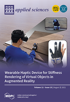
For realistic finger-based object manipulation in augmented reality (AR), haptic rendering of object stiffness is important yet challenging due to the co-presence of real hands, haptic devices, and rendered AR objects. Thus, we propose a novel wearable haptic device, which can generate rigid and elastic haptic feedback in a small form-factor with a simple mechanism to minimize occlusions in the AR scene. Through human-subject experiments in AR, the efficacy of our proposed haptic device is verified/compared against other feedbacks (vibrotactile, visual) for stiffness rendering. View this paper
  • Issues are regarded as officially published after their release is announced to the table of contents alert mailing list.
  • You may sign up for e-mail alerts to receive table of contents of newly released issues.
  • PDF is the official format for papers published in both, html and pdf forms. To view the papers in pdf format, click on the "PDF Full-text" link, and use the free Adobe Reader to open them.
Order results
Result details
Section
Select all
Export citation of selected articles as:
16 pages, 4547 KiB  
Article
Radiological Dose Assessment of the Landfill Disposal of Consumer Products Containing Naturally Occurring Radioactive Materials in South Korea
by Mercy Nandutu and Juyoul Kim
Appl. Sci. 2021, 11(15), 7172; https://doi.org/10.3390/app11157172 - 3 Aug 2021
Cited by 1 | Viewed by 2760
Abstract
Naturally occurring radioactive materials (NORMs) are long-lived radioactive elements such as uranium, thorium, and potassium, and theirdecay products. They are abundant in natural rocks and minerals. In this study, we conducted a radiological dose assessment of the disposal of consumer products (CPs) containing [...] Read more.
Naturally occurring radioactive materials (NORMs) are long-lived radioactive elements such as uranium, thorium, and potassium, and theirdecay products. They are abundant in natural rocks and minerals. In this study, we conducted a radiological dose assessment of the disposal of consumer products (CPs) containing NORMs at landfills and incinerators in South Korea. Household wastes were categorized as combustible and noncombustible on the basis of activity concentrations (ACs) ranging below and above 1 Bq/g, respectively. Analysis data were obtained from previous literature and the Nuclear Safety and Security Commission (NSSC) of South Korea, and statistical analysis was performed using an interval plot and 95% confidence interval of mean for each category as an input. Using RESRAD computer codes for noncombustible CPs with AC below and above 1 Bq/g, we found out that the dose rate was below and above 1 mSv/y, respectively. The RESRAD-OFFSITE results showed that the dose incurred during the study period for both ranges of AC was all below the public dose limit of 1 mSv/y. NORM and LegacY Site Assessment (NORMALYSA) code was used to validate the result of the RESRAD-ONSITE code, and the results showed that the dose was equal to and above 1 mSv/y for ACs below and above 1 Bq/g, respectively. HotSpot code was used for dose evaluation to offsite residents from incineration of combustible CPs, and the resulting dose was below 1 mSv/y. These findings can be used as a guideline for managing public exposure from landfill sites with varying ACs ranges. Therefore, the competent authority should ensure that criteria and protection measures are established for people who live within a distance of 10 km from incinerators and landfill sites that are contaminated with consumer products containing NORMs. Full article
(This article belongs to the Section Environmental Sciences)
Show Figures

Figure 1

Figure 1
<p>95% confidence interval for the mean activity concentration of <sup>238</sup>U, <sup>232</sup>Th, and <sup>40</sup>K (Bq/g).</p>
Full article ">Figure 2
<p>Summary of the scenario for the disposal of consumer products containing naturally occurring radioactive materials.</p>
Full article ">Figure 3
<p>Main libraries in NORM and LegacY Site Assessment.</p>
Full article ">Figure 4
<p>Results from RESRAD ONSITE scenario.</p>
Full article ">Figure 5
<p>Dose from the RESRAD-OFFSITE scenario.</p>
Full article ">Figure 6
<p>Dose from the HotSpot code for activity concentration below 1000 Bq/kg.</p>
Full article ">Figure 7
<p>Dose from the HotSpot code for activity concentration above 1000 Bq/kg.</p>
Full article ">Figure 8
<p>Dose from the NORM and LegacY Site Assessment code.</p>
Full article ">Figure 9
<p>Comparison graph for the four computer codes.</p>
Full article ">
15 pages, 12213 KiB  
Article
Optimizing Power and Thermal Efficiency of an Irreversible Variable-Temperature Heat Reservoir Lenoir Cycle
by Ruibo Wang, Lingen Chen, Yanlin Ge and Huijun Feng
Appl. Sci. 2021, 11(15), 7171; https://doi.org/10.3390/app11157171 - 3 Aug 2021
Cited by 17 | Viewed by 2156
Abstract
Applying finite-time thermodynamics theory, an irreversible steady flow Lenoir cycle model with variable-temperature heat reservoirs is established, the expressions of power (P) and efficiency (η) are derived. By numerical calculations, the characteristic relationships among P and η and the [...] Read more.
Applying finite-time thermodynamics theory, an irreversible steady flow Lenoir cycle model with variable-temperature heat reservoirs is established, the expressions of power (P) and efficiency (η) are derived. By numerical calculations, the characteristic relationships among P and η and the heat conductance distribution (uL) of the heat exchangers, as well as the thermal capacity rate matching (Cwf1/CH) between working fluid and heat source are studied. The results show that when the heat conductances of the hot- and cold-side heat exchangers (UH, UL) are constants, P-η is a certain “point”, with the increase of heat reservoir inlet temperature ratio (τ), UH, UL, and the irreversible expansion efficiency (ηe), P and η increase. When uL can be optimized, P and η versus uL characteristics are parabolic-like ones, there are optimal values of heat conductance distributions (uLP(opt), uLη(opt)) to make the cycle reach the maximum power and efficiency points (Pmax, ηmax). As Cwf1/CH increases, Pmax-Cwf1/CH shows a parabolic-like curve, that is, there is an optimal value of Cwf1/CH ((Cwf1/CH)opt) to make the cycle reach double-maximum power point ((Pmax)max); as CL/CH, UT, and ηe increase, (Pmax)max and (Cwf1/CH)opt increase; with the increase in τ, (Pmax)max increases, and (Cwf1/CH)opt is unchanged. Full article
(This article belongs to the Topic Exergy Analysis and Its Applications)
Show Figures

Figure 1

Figure 1
<p>Cycle <math display="inline"><semantics> <mrow> <mi>T</mi> <mtext>-</mtext> <mi>s</mi> </mrow> </semantics></math> diagram.</p>
Full article ">Figure 2
<p>The characteristic of <math display="inline"><semantics> <mrow> <mi>P</mi> <mtext>-</mtext> <mi>η</mi> </mrow> </semantics></math> (<b>a</b>) and the influence of <math display="inline"><semantics> <mrow> <msub> <mi>η</mi> <mi>e</mi> </msub> </mrow> </semantics></math> on <math display="inline"><semantics> <mrow> <mi>P</mi> <mtext>-</mtext> <mi>η</mi> </mrow> </semantics></math> characteristics when <math display="inline"><semantics> <mrow> <msub> <mi>U</mi> <mi>H</mi> </msub> </mrow> </semantics></math> and <math display="inline"><semantics> <mrow> <msub> <mi>U</mi> <mi>L</mi> </msub> </mrow> </semantics></math> are given (<b>b</b>).</p>
Full article ">Figure 3
<p>The curve of <math display="inline"><semantics> <mrow> <mi>P</mi> <mtext>-</mtext> <msub> <mi>u</mi> <mi>L</mi> </msub> </mrow> </semantics></math>.</p>
Full article ">Figure 4
<p>The curve of <math display="inline"><semantics> <mrow> <mi>η</mi> <mtext>-</mtext> <msub> <mi>u</mi> <mi>L</mi> </msub> </mrow> </semantics></math>.</p>
Full article ">Figure 5
<p>The characteristics of <math display="inline"><semantics> <mrow> <msub> <mi>P</mi> <mrow> <mi>max</mi> </mrow> </msub> <mtext>-</mtext> <msub> <mi>U</mi> <mi>T</mi> </msub> </mrow> </semantics></math> and <math display="inline"><semantics> <mrow> <msub> <mi>u</mi> <mi>L</mi> </msub> <msub> <mrow> <msub> <mrow/> <mrow> <msub> <mrow/> <mi>P</mi> </msub> </mrow> </msub> </mrow> <mrow> <mo>(</mo> <mi>o</mi> <mi>p</mi> <mi>t</mi> <mo>)</mo> </mrow> </msub> <mtext>-</mtext> <msub> <mi>U</mi> <mi>T</mi> </msub> </mrow> </semantics></math> about <math display="inline"><semantics> <mi>τ</mi> </semantics></math>.</p>
Full article ">Figure 6
<p>The characteristics of <math display="inline"><semantics> <mrow> <msub> <mi>η</mi> <mrow> <mi>max</mi> </mrow> </msub> <mtext>-</mtext> <msub> <mi>U</mi> <mi>T</mi> </msub> </mrow> </semantics></math> and <math display="inline"><semantics> <mrow> <msub> <mi>u</mi> <mi>L</mi> </msub> <msub> <mrow> <msub> <mrow/> <mrow> <msub> <mrow/> <mi>η</mi> </msub> </mrow> </msub> </mrow> <mrow> <mo>(</mo> <mi>o</mi> <mi>p</mi> <mi>t</mi> <mo>)</mo> </mrow> </msub> <mtext>-</mtext> <msub> <mi>U</mi> <mi>T</mi> </msub> </mrow> </semantics></math> about <math display="inline"><semantics> <mi>τ</mi> </semantics></math>.</p>
Full article ">Figure 7
<p>The characteristics of <math display="inline"><semantics> <mrow> <msub> <mi>P</mi> <mrow> <mi>max</mi> </mrow> </msub> <mtext>-</mtext> <msub> <mi>η</mi> <mi>e</mi> </msub> </mrow> </semantics></math> and <math display="inline"><semantics> <mrow> <msub> <mi>u</mi> <mi>L</mi> </msub> <msub> <mrow> <msub> <mrow/> <mrow> <msub> <mrow/> <mi>P</mi> </msub> </mrow> </msub> </mrow> <mrow> <mo>(</mo> <mi>o</mi> <mi>p</mi> <mi>t</mi> <mo>)</mo> </mrow> </msub> <mtext>-</mtext> <msub> <mi>η</mi> <mi>e</mi> </msub> </mrow> </semantics></math>.</p>
Full article ">Figure 8
<p>The characteristics of <math display="inline"><semantics> <mrow> <msub> <mi>η</mi> <mrow> <mi>max</mi> </mrow> </msub> <mtext>-</mtext> <msub> <mi>η</mi> <mi>e</mi> </msub> </mrow> </semantics></math> and <math display="inline"><semantics> <mrow> <msub> <mi>u</mi> <mi>L</mi> </msub> <msub> <mrow> <msub> <mrow/> <mrow> <msub> <mrow/> <mi>η</mi> </msub> </mrow> </msub> </mrow> <mrow> <mo>(</mo> <mi>o</mi> <mi>p</mi> <mi>t</mi> <mo>)</mo> </mrow> </msub> <mtext>-</mtext> <msub> <mi>η</mi> <mi>e</mi> </msub> </mrow> </semantics></math>.</p>
Full article ">Figure 9
<p>The characteristics of <math display="inline"><semantics> <mrow> <msub> <mi>P</mi> <mrow> <mi>max</mi> </mrow> </msub> <mtext>-</mtext> <msub> <mi>C</mi> <mrow> <mi>w</mi> <mi>f</mi> <mn>1</mn> </mrow> </msub> <mo>/</mo> <msub> <mi>C</mi> <mi>H</mi> </msub> </mrow> </semantics></math> about <math display="inline"><semantics> <mrow> <msub> <mi>C</mi> <mi>L</mi> </msub> <mo>/</mo> <msub> <mi>C</mi> <mi>H</mi> </msub> </mrow> </semantics></math>.</p>
Full article ">Figure 10
<p>The characteristics of <math display="inline"><semantics> <mrow> <msub> <mi>P</mi> <mrow> <mi>max</mi> </mrow> </msub> <mtext>-</mtext> <msub> <mi>C</mi> <mrow> <mi>w</mi> <mi>f</mi> <mn>1</mn> </mrow> </msub> <mo>/</mo> <msub> <mi>C</mi> <mi>H</mi> </msub> </mrow> </semantics></math> about <math display="inline"><semantics> <mrow> <msub> <mi>U</mi> <mi>T</mi> </msub> </mrow> </semantics></math>.</p>
Full article ">Figure 11
<p>The characteristics of <math display="inline"><semantics> <mrow> <msub> <mi>P</mi> <mrow> <mi>max</mi> </mrow> </msub> <mtext>-</mtext> <msub> <mi>C</mi> <mrow> <mi>w</mi> <mi>f</mi> <mn>1</mn> </mrow> </msub> <mo>/</mo> <msub> <mi>C</mi> <mi>H</mi> </msub> </mrow> </semantics></math> about <math display="inline"><semantics> <mi>τ</mi> </semantics></math>.</p>
Full article ">Figure 12
<p>The characteristics of <math display="inline"><semantics> <mrow> <msub> <mi>P</mi> <mrow> <mi>max</mi> </mrow> </msub> <mtext>-</mtext> <msub> <mi>C</mi> <mrow> <mi>w</mi> <mi>f</mi> <mn>1</mn> </mrow> </msub> <mo>/</mo> <msub> <mi>C</mi> <mi>H</mi> </msub> </mrow> </semantics></math> about <math display="inline"><semantics> <mrow> <msub> <mi>η</mi> <mi>e</mi> </msub> </mrow> </semantics></math>.</p>
Full article ">
13 pages, 11413 KiB  
Article
Integer Search Algorithm: A New Discrete Multi-Objective Algorithm for Pavement Maintenance Management Optimization
by Abdulraaof Alqaili, Mohammed Qais and Abdullah Al-Mansour
Appl. Sci. 2021, 11(15), 7170; https://doi.org/10.3390/app11157170 - 3 Aug 2021
Cited by 7 | Viewed by 2270
Abstract
Optimization techniques keep road performance at a good level using a cost-effective maintenance strategy. Thus, the trade-off between cost and road performance is a multi-objective function. This paper offers a new multi-objective stochastic algorithm for discrete variables, which is called the integer search [...] Read more.
Optimization techniques keep road performance at a good level using a cost-effective maintenance strategy. Thus, the trade-off between cost and road performance is a multi-objective function. This paper offers a new multi-objective stochastic algorithm for discrete variables, which is called the integer search algorithm (ISA). This algorithm is applied to an optimal pavement maintenance management system (PMMS), where the variables are discrete. The PMMS optimization can be achieved by maximizing the condition of pavement with a minimum cost at specified constraints, so the PMMS is a constrained multi-objective problem. The ISA and genetic algorithm (GA) are applied to improve the performance condition rating (PCR) of the pavement in developing countries, where the annual budget is limited, so a minimum cost for three years’ maintenance is scheduled. Study results revealed that the ISA produced an optimal solution for multi-function objectives better than the optimal solution of GA. Full article
(This article belongs to the Topic Applied Metaheuristic Computing)
Show Figures

Figure 1

Figure 1
<p>Flowchart of the integer search algorithm.</p>
Full article ">Figure 2
<p>Pseudo-code of PCR initialization.</p>
Full article ">Figure 3
<p>Pseudo-code of the application of the ISA algorithm for PMMS problem.</p>
Full article ">Figure 4
<p>Convergence of the cumulative PCR for 3 years and 49 sections.</p>
Full article ">Figure 5
<p>Convergence of the cumulative maintenance cost for 3 years and 49 sections.</p>
Full article ">Figure 6
<p>Improvement of PCR.</p>
Full article ">Figure 7
<p>Annual maintenance cost during three years.</p>
Full article ">Figure 8
<p>Range and standard deviation of PCR.</p>
Full article ">Figure 9
<p>Optimal distribution of maintenance activities.</p>
Full article ">Figure 10
<p>Optimal distribution of maintenance activities for road classes.</p>
Full article ">
17 pages, 27593 KiB  
Article
Lightweight Blockchain Processing. Case Study: Scanned Document Tracking on Tezos Blockchain
by Mohamed Allouche, Tarek Frikha, Mihai Mitrea, Gérard Memmi and Faten Chaabane
Appl. Sci. 2021, 11(15), 7169; https://doi.org/10.3390/app11157169 - 3 Aug 2021
Cited by 23 | Viewed by 3385
Abstract
To bridge the current gap between the Blockchain expectancies and their intensive computation constraints, the present paper advances a lightweight processing solution, based on a load-balancing architecture, compatible with the lightweight/embedding processing paradigms. In this way, the execution of complex operations is securely [...] Read more.
To bridge the current gap between the Blockchain expectancies and their intensive computation constraints, the present paper advances a lightweight processing solution, based on a load-balancing architecture, compatible with the lightweight/embedding processing paradigms. In this way, the execution of complex operations is securely delegated to an off-chain general-purpose computing machine while the intimate Blockchain operations are kept on-chain. The illustrations correspond to an on-chain Tezos configuration and to a multiprocessor ARM embedded platform (integrated into a Raspberry Pi). The performances are assessed in terms of security, execution time, and CPU consumption when achieving a visual document fingerprint task. It is thus demonstrated that the advanced solution makes it possible for a computing intensive application to be deployed under severely constrained computation and memory resources, as set by a Raspberry Pi 3. The experimental results show that up to nine Tezos nodes can be deployed on a single Raspberry Pi 3 and that the limitation is not derived from the memory but from the computation resources. The execution time with a limited number of fingerprints is 40% higher than using a classical PC solution (value computed with 95% relative error lower than 5%). Full article
(This article belongs to the Special Issue Advances in Blockchain Technology and Applications II)
Show Figures

Figure 1

Figure 1
<p>Digital documents: heterogeneous content (text, image, etc.) with various digital representations for the same semantic content.</p>
Full article ">Figure 2
<p>Tezos Smart Contract Workflow.</p>
Full article ">Figure 3
<p>On-chain/off-chain code balancing.</p>
Full article ">Figure 4
<p>Task allocations on the two computing devices.</p>
Full article ">Figure 5
<p>Execution sequence diagram.</p>
Full article ">Figure 6
<p>Original images sampled from database.</p>
Full article ">Figure 7
<p>Attacked images sampled from database.</p>
Full article ">Figure 8
<p>Memory consumption depends on nodes number.</p>
Full article ">Figure 9
<p>System crashes with more than nine nodes.</p>
Full article ">Figure 10
<p>Nodes and groups of nodes can be hosted on different computing resources, from PCs to Raspberry Pi.</p>
Full article ">
12 pages, 10400 KiB  
Article
Flow Control Techniques for Enhancing the Bio-Recognition Performance of Microfluidic-Integrated Biosensors
by Fatemeh Shahbazi, Mohammad Souri, Masoud Jabbari and Amir Keshmiri
Appl. Sci. 2021, 11(15), 7168; https://doi.org/10.3390/app11157168 - 3 Aug 2021
Cited by 3 | Viewed by 2321
Abstract
Biosensors are favored devices for the fast and cost-effective detection of biological species without the need for laboratories. Microfluidic integration with biosensors has advanced their capabilities in selectivity, sensitivity, controllability, and conducting multiple binding assays simultaneously. Despite all the improvements, their design and [...] Read more.
Biosensors are favored devices for the fast and cost-effective detection of biological species without the need for laboratories. Microfluidic integration with biosensors has advanced their capabilities in selectivity, sensitivity, controllability, and conducting multiple binding assays simultaneously. Despite all the improvements, their design and fabrication are still challenging and time-consuming. The current study aims to enhance microfluidic-integrated biosensors’ performance. Three different functional designs are presented with both active (with the help of electroosmotic flow) and passive (geometry optimization) methods. For validation and further studies, these solutions are applied to an experimental setup for DNA hybridization. The numerical results for the original case have been validated with the experimental data from previous literature. Convection, diffusion, migration, and hybridization of DNA strands during the hybridization process have been simulated with finite element method (FEM) in 3D. Based on the results, increasing the velocity on top of the functionalized surface, by reducing the thickness of the microchamber in that area, would increase the speed of surface coverage by up to 62%. An active flow control with the help of electric field would increase this speed by 32%. In addition, other essential parameters in the fabrication of the microchamber, such as changes in pressure and bulk concentration, have been studied. The suggested designs are simple, applicable and cost-effective, and would not add extra challenges to the fabrication process. Overall, the effect of the geometry of the microchamber on the time and effectiveness of biosensors is inevitable. More studies on the geometry optimization of the microchamber and position of the electrodes using machine learning methods would be beneficial in future works. Full article
(This article belongs to the Special Issue Fluid Flows Modelling in Microfluidic Systems)
Show Figures

Figure 1

Figure 1
<p>Bio-recognition process for DNA hybridization in a microchamber equipped with four functionalized surfaces for recognizing a specific sequence, dissociation of the double helix structure of the DNA, and hybridization with the functionalized surface.</p>
Full article ">Figure 2
<p>The time-dependent solution from the beginning of the test (<math display="inline"><semantics> <mrow> <msub> <mi>t</mi> <mn>0</mn> </msub> </mrow> </semantics></math>) to 50 <math display="inline"><semantics> <mrow> <mi>min</mi> </mrow> </semantics></math> (<math display="inline"><semantics> <mrow> <msub> <mi>t</mi> <mn>1</mn> </msub> </mrow> </semantics></math>), and 150 <math display="inline"><semantics> <mrow> <mi>min</mi> </mrow> </semantics></math> (<math display="inline"><semantics> <mrow> <msub> <mi>t</mi> <mn>2</mn> </msub> </mrow> </semantics></math>) [<a href="#B28-applsci-11-07168" class="html-bibr">28</a>].</p>
Full article ">Figure 3
<p>Concentration contour for the original case (A-01) at the start of the time (<b>a</b>), after 50 s (<b>b</b>), after 150 s (<b>c</b>), and at the end of 50 min (<b>d</b>).</p>
Full article ">Figure 4
<p>The time-dependent solution for surface coverage of the original experimental setup (Case A) in comparison to cases H-03, S-04, and E06 for the whole surface (<b>a</b>), <math display="inline"><semantics> <mrow> <mi>P</mi> <msub> <mi>t</mi> <mi>f</mi> </msub> </mrow> </semantics></math> (<b>b</b>) and <math display="inline"><semantics> <mrow> <mi>P</mi> <msub> <mi>t</mi> <mi>b</mi> </msub> </mrow> </semantics></math> (<b>c</b>). A slide of surface concentration contour on the functionalized surfaces for cases A-01, H-03, S-04, and E06, after 100 <math display="inline"><semantics> <mi>s</mi> </semantics></math> (<b>d</b>), 750 <math display="inline"><semantics> <mi>s</mi> </semantics></math> (<b>e</b>), 2000 <math display="inline"><semantics> <mi>s</mi> </semantics></math> (<b>f</b>) and 3000 <math display="inline"><semantics> <mi>s</mi> </semantics></math> (<b>g</b>).</p>
Full article ">Figure 5
<p>The time-dependent solution for surface concentration in the first 50 <math display="inline"><semantics> <mrow> <mi>min</mi> </mrow> </semantics></math> for the original experimental setup (Case A) in comparison to the: thin chamber (<b>a</b>), suction (<b>b</b>), and electroosmotic flow (<b>c</b>). A slide of bulk concentration on the functionalized surfaces for cases A-01, H-03, S-04, and E06, after 100 <math display="inline"><semantics> <mi>s</mi> </semantics></math> (<b>d</b>) and 3000 <math display="inline"><semantics> <mi>s</mi> </semantics></math> (<b>e</b>).</p>
Full article ">Figure 6
<p>The coverage speed and maximum coverage after 50 <math display="inline"><semantics> <mrow> <mi>min</mi> </mrow> </semantics></math> and 150 <math display="inline"><semantics> <mrow> <mi>min</mi> </mrow> </semantics></math> through the microchamber for the original experimental setup (case A-01), thin chamber (series H-02), the thin chamber with half-height (case H-03), second outlet with zero pressure (case S-04), suction (case S-05), and electroosmotic flow (cases E-06 and E-07). All values are calculated based on the original case.</p>
Full article ">Figure 7
<p>The maximum pressure through the microchamber for the original experimental setup (case A-01), thin chamber (series H-02), the thin chamber with half-height (case H-03), second outlet with zero pressure (case S-04), suction (case S-05), electroosmotic flow (cases E-06 and E-07).</p>
Full article ">
23 pages, 9864 KiB  
Article
Large-Eddy Simulation Study of Flow and Heat Transfer in Swirling and Non-Swirling Impinging Jets on a Semi-Cylinder Concave Target
by Liang Xu, Xu Zhao, Lei Xi, Yonghao Ma, Jianmin Gao and Yunlong Li
Appl. Sci. 2021, 11(15), 7167; https://doi.org/10.3390/app11157167 - 3 Aug 2021
Cited by 6 | Viewed by 2467
Abstract
Swirling impinging jet (SIJ) is considered as an effective means to achieve uniform cooling at high heat transfer rates, and the complex flow structure and its mechanism of enhancing heat transfer have attracted much attention in recent years. The large eddy simulation (LES) [...] Read more.
Swirling impinging jet (SIJ) is considered as an effective means to achieve uniform cooling at high heat transfer rates, and the complex flow structure and its mechanism of enhancing heat transfer have attracted much attention in recent years. The large eddy simulation (LES) technique is employed to analyze the flow fields of swirling and non-swirling impinging jet emanating from a hole with four spiral and straight grooves, respectively, at a relatively high Reynolds number (Re) of 16,000 and a small jet spacing of H/D = 2 on a concave surface with uniform heat flux. Firstly, this work analyzes two different sub-grid stress models, and LES with the wall-adapting local eddy-viscosity model (WALEM) is established for accurately predicting flow and heat transfer performance of SIJ on a flat surface. The complex flow field structures, spectral characteristics, time-averaged flow characteristics and heat transfer on the target surface for the swirling and non-swirling impinging jets are compared in detail using the established method. The results show that small-scale recirculation vortices near the wall change the nearby flow into an unstable microwave state, resulting in small-scale fluctuation of the local Nusselt number (Nu) of the wall. There is a stable recirculation vortex at the stagnation point of the target surface, and the axial and radial fluctuating speeds are consistent with the fluctuating wall temperature. With the increase in the radial radius away from the stagnation point, the main frequency of the fluctuation of wall temperature coincides with the main frequency of the fluctuation of radial fluctuating velocity at x/D = 0.5. Compared with 0° straight hole, 45° spiral hole has a larger fluctuating speed because of speed deflection, resulting in a larger turbulence intensity and a stronger air transport capacity. The heat transfer intensity of the 45° spiral hole on the target surface is slightly improved within 5–10%. Full article
(This article belongs to the Section Mechanical Engineering)
Show Figures

Figure 1

Figure 1
<p>Computational domains and grid of a swirling impinging jet on a flat target: (<b>a</b>) computational domains, (<b>b</b>) computational grid.</p>
Full article ">Figure 2
<p>(<b>a</b>) Mean radial velocity and (<b>b</b>) turbulent kinetic energy at <span class="html-italic">r/D</span> = 2.</p>
Full article ">Figure 3
<p>The ratio of the sub-grid viscosity to the molecular viscosity at <span class="html-italic">r</span>/<span class="html-italic">D</span> = 0 and <span class="html-italic">r</span>/<span class="html-italic">D</span> = 1; (<b>a</b>) <span class="html-italic">r</span>/<span class="html-italic">D</span> = 0; (<b>b</b>) <span class="html-italic">r</span>/<span class="html-italic">D</span> = 1.</p>
Full article ">Figure 4
<p>Radial distribution of <span class="html-italic">Nu</span> at the flat target wall.</p>
Full article ">Figure 5
<p>Geometrical structure and computational domains.</p>
Full article ">Figure 6
<p>The contours of the instantaneous axial velocity in the XOY and YOZ planes.</p>
Full article ">Figure 7
<p>The distribution of pressure in the XOY and YOZ planes.</p>
Full article ">Figure 8
<p>Streamlines and velocity vectors in the XOY and YOZ planes.</p>
Full article ">Figure 9
<p>Instantaneous iso-Q-criterion surface for the MCIJ and SIJ.</p>
Full article ">Figure 10
<p>The mean second invariant in jet space at <span class="html-italic">y/D</span> = 0.05 along the <span class="html-italic">x</span> direction.</p>
Full article ">Figure 11
<p>Power spectral density of the axial fluctuating velocity in jet space.</p>
Full article ">Figure 12
<p>Power spectral density of radial fluctuating velocity near the target surface.</p>
Full article ">Figure 13
<p>The distribution of axial time-averaged velocity at different positions.</p>
Full article ">Figure 14
<p>Distribution of root mean square of the axial and radial fluctuating velocities.</p>
Full article ">Figure 15
<p>Cloud plot of the distribution of instantaneous <span class="html-italic">Nu</span> number ratio on the target surface.</p>
Full article ">Figure 16
<p>The distribution of <span class="html-italic">Nu/Nu<sub>st</sub></span> in the <span class="html-italic">x</span> direction.</p>
Full article ">Figure 17
<p>Temperature distribution of near-wall in the jet core and wall jet regions.</p>
Full article ">Figure 18
<p>Spectrum of temperature fluctuations at different positions on the impact target surface.</p>
Full article ">
13 pages, 1228 KiB  
Article
The Influence of Hard- and Software Improvement of Intraoral Scanners on the Implant Transfer Accuracy from 2012 to 2021: An In Vitro Study
by Alexander Schmidt, Maximiliane Amelie Schlenz, Haoyu Liu, Holger Sebastian Kämpe and Bernd Wöstmann
Appl. Sci. 2021, 11(15), 7166; https://doi.org/10.3390/app11157166 - 3 Aug 2021
Cited by 10 | Viewed by 3001
Abstract
This study aimed to investigate the transfer accuracy (trueness and precision) of three different intraoral scanning families using different hardware and software versions over the last decade from 2012 to 2021, compared to a conventional impression. Therefore, an implant master model with a [...] Read more.
This study aimed to investigate the transfer accuracy (trueness and precision) of three different intraoral scanning families using different hardware and software versions over the last decade from 2012 to 2021, compared to a conventional impression. Therefore, an implant master model with a reference cube was digitized and served as a reference dataset. Digital impressions of all three scanning families (True definition, TRIOS, CEREC) were recorded (n = 10 per group), and conventional implant impressions were taken (n = 10). The conventional models were digitized, and all models (conventional and digital) were measured. Therefore, it was possible to obtain the deviations between the master model and the scans or conventional models in terms of absolute three-dimensional (3D) deviations, deviations in rotation, and angulation. The results for deviations between the older and newer scanning systems were analyzed using pairwise comparisons (p < 0.05; SPSS 26). The absolute 3D deviations increased with increasing scan path length, particularly for the older hardware and software versions (old vs. new (MW ± SD) True Definition: 355 ± 62 µm vs. 483 ± 110 µm; TRIOS: 574 ± 274 µm vs. 258 ± 100 µm; and CEREC: 1356 ± 1023 µm vs. 110 ± 49 µm). This was also true for deviations in rotation and angulation. The conventional impression showed an advantage only regarding the absolute 3D deviation compared to the older systems. Based on the data of the present study, the accuracy of intraoral scanners is decisively related to hardware and software; though, newer systems or software do not necessarily warrant improvement. Nevertheless, to achieve high transfer accuracy, regular updating of digital systems is recommended. The challenge of increasing errors with increasing scan paths is overcome in the most recent systems. The combination of two different scanning principles in a single device seems to be beneficial. Full article
(This article belongs to the Special Issue Clinical Applications for Dentistry and Oral Health)
Show Figures

Figure 1

Figure 1
<p>Implant master model (IMM) with two reference cubes and final setup with inserted scan bodies (FDI 16, 14, 25, 26).</p>
Full article ">Figure 2
<p>Schematic representation of the measured absolute three-dimensional distances (<b>A</b>), rotations (<b>B</b>), and angulations (<b>C</b>) within the implant master model (IMM).</p>
Full article ">Figure 3
<p>Results for the absolute three-dimensional deviations for the implant positions for each intraoral scanner (TD_4.1: True Definition scanner (Cart version) 4.1; TD_5.4: True Definition scanner (Cart version) 5.4; TDpb_5.4: True Definition scanner (Portable version) 5.4; TR2: TRIOS II; TR 4: TRIOS 4; OC_4.2: CEREC Omnicam 4.2.1.61068; OC_4.6: CEREC Omnicam 4.6.1.152739; and PS: CEREC Primescan 5.1.0.190461).</p>
Full article ">Figure 4
<p>Results for the rotational deviations for the implant positions for each intraoral scanner (TD_4.1: True Definition scanner (Cart version) 4.1; TD_5.4: True Definition scanner (Cart version) 5.4; TDpb_5.4: True Definition scanner (Portable version) 5.4; TR2: TRIOS II; TR 4: TRIOS 4; OC_4.2: CEREC Omnicam 4.2.1.61068; OC_4.6: CEREC Omnicam 4.6.1.152739; and PS: CEREC Primescan 5.1.0.190461).</p>
Full article ">Figure 5
<p>Results for the angulation deviations for the implant positions for each intraoral scanner (TD_4.1: True Definition scanner (Cart version) 4.1; TD_5.4: True Definition scanner (Cart version) 5.4; TDpb_5.4: True Definition scanner (Portable version) 5.4; TR2: TRIOS II; TR 4: TRIOS 4; OC_4.2: CEREC Omnicam 4.2.1.61068; OC_4.6: CEREC Omnicam 4.6.1.152739; and PS: CEREC Primescan 5.1.0.190461).</p>
Full article ">
11 pages, 6205 KiB  
Article
A Form-Finding Method for Branching Structures Based on Dynamic Relaxation
by Guigang Tu, Chen Chen, Zaijing Gong and Yueren Wang
Appl. Sci. 2021, 11(15), 7165; https://doi.org/10.3390/app11157165 - 3 Aug 2021
Cited by 4 | Viewed by 2924
Abstract
Branching structure is often used as a supporting structure of the grid shell due to its geometrical and force-transferring features, and the rationality of its shape is very important. The “physical” and “numerical” hanging models can be used for the joint form-finding of [...] Read more.
Branching structure is often used as a supporting structure of the grid shell due to its geometrical and force-transferring features, and the rationality of its shape is very important. The “physical” and “numerical” hanging models can be used for the joint form-finding of the branching structure and free-form grid shell. However, slack elements may exist in the equilibrium model which corresponds to the inefficient members in the form-found branching structure. To solve this problem, a form-finding method of branching structure based on dynamic relaxation is proposed in this study. The proposed method clusters the elements of the branching model and equalizes the axial forces of the elements in the same cluster, in other words, there are no slack elements in the equilibrium branching model. This method overcomes the defect that the equilibrium branching model may have slack elements and needs many manual adjustments during the procedure of determining the rational shape of a branching structure, and effectively prevents the inefficient members existing in the form-found structure. Numerical examples are provided to demonstrate the characteristics of the proposed method and its effectiveness is verified as well. Full article
(This article belongs to the Section Civil Engineering)
Show Figures

Figure 1

Figure 1
<p>Shape schemes of different element clusters. (<b>a</b>) initial flexible model; (<b>b</b>) form-found shape of traditional DR method; (<b>c</b>,<b>d</b>) form-found shapes of element-clustered method.</p>
Full article ">Figure 2
<p>Initial hanging model.</p>
Full article ">Figure 3
<p>Comparison of the form-found structures. (<b>a</b>) the whole structure and (<b>c</b>) branching structure generated by traditional DR method; (<b>b</b>) the whole structure and (<b>d</b>) branching structure generated by element-clustered method</p>
Full article ">Figure 4
<p>Comparison of the branching structures generated by two methods.</p>
Full article ">Figure 5
<p>Comparison of mechanical properties of form-found structures. Bending moment distributions of the structures generated by (<b>a</b>) traditional DR method and (<b>b</b>) element-clustered method; Nodal displacement distributions of the structures generated by (<b>c</b>) traditional DR method and (<b>d</b>) element-clustered method; Axial force distributions of branching structures generated by (<b>e</b>) traditional DR method and (<b>f</b>) element-clustered method.</p>
Full article ">Figure 6
<p>Comparison of axial forces in the members of branching structures.</p>
Full article ">
16 pages, 4817 KiB  
Article
Target Maintenance in Gaming via Saliency Augmentation: An Early-Stage Scotoma Simulation Study Using Virtual Reality (VR)
by Alexandra Sipatchin, Miguel García García and Siegfried Wahl
Appl. Sci. 2021, 11(15), 7164; https://doi.org/10.3390/app11157164 - 3 Aug 2021
Cited by 6 | Viewed by 3028
Abstract
This study addresses the importance of salience placement before or after scotoma development for an efficient target allocation in the visual field. Pre-allocation of attention is a mechanism known to induce a better gaze positioning towards the target. Three different conditions were tested: [...] Read more.
This study addresses the importance of salience placement before or after scotoma development for an efficient target allocation in the visual field. Pre-allocation of attention is a mechanism known to induce a better gaze positioning towards the target. Three different conditions were tested: a simulated central scotoma, a salience augmentation surrounding the scotoma and a baseline condition without any simulation. All conditions were investigated within a virtual reality VR gaming environment. Participants were tested in two different orders, either the salient cue was applied together with the scotoma before being presented with the scotoma alone or the scotoma in the wild was presented before and, then, with the augmentation around it. Both groups showed a change in gaze behaviour when saliency was applied. However, in the second group, salient augmentation also induced changes in gaze behaviour for the scotoma condition without augmentation, gazing above and outside the scotoma following previous literature. These preliminary results indicate salience placement before developing an advanced stage of scotoma can induce effective and rapid training for efficient target maintenance during VR gaming. The study shows the potential of salience and VR gaming as therapy for early AMD patients. Full article
(This article belongs to the Special Issue Serious Games and Mixed Reality Applications for Healthcare)
Show Figures

Figure 1

Figure 1
<p>(<b>a</b>) Specifications of the central scotoma (CS) and (<b>b</b>) augmented scotoma (AS) condition. In the CS condition the scotoma (<b>a</b>) had a diameter of 12<math display="inline"><semantics> <msup> <mrow/> <mo>∘</mo> </msup> </semantics></math>. In the AS condition (<b>b</b>) there was an concentric augmentation of 2<math display="inline"><semantics> <msup> <mrow/> <mo>∘</mo> </msup> </semantics></math> around the scotoma and an annulus area extending <math display="inline"><semantics> <mrow> <mn>7.5</mn> </mrow> </semantics></math><math display="inline"><semantics> <msup> <mrow/> <mo>∘</mo> </msup> </semantics></math>.</p>
Full article ">Figure 2
<p>Drift correction was performed manually by the subject to have a centralized scotoma around the red dot at the beginning of each block. In the figure above, a hypothetical example of how a decentralized scotoma (in black) might look like (<b>a</b>) and hypothetical stages of position correction (<b>b</b>,<b>c</b>), black arrows, performed to have a concentric positioning of the scotoma around the red dot (<b>c</b>). The grey circle is used as a reference for this figure to indicate where the simulated scotoma should be positioned.</p>
Full article ">Figure 3
<p>Scheme of the experimental procedure. Participants were divided into two groups (G1 and G2). Both groups initiated playing the Pong game under normal vision conditions (normally sighted, NS). The difference between groups was defined by the order by which the scotoma (CS) and augmented scotoma (AS) simulations were presented. In group 1, the scotoma simulation followed the augmentation, in group 2 the opposite. During each condition, three blocks (1, 2, and 3) were tested. Each block was the same for all conditions. It started with a manual drift correction followed by a 5-min timer playtime. During the game, the ball could have exited the play area. In that case, the timer was frozen and the game re-started. When the timer ended, a new block started.</p>
Full article ">Figure 4
<p>Latency offset for best gaze-target distance across all subjects. The red line indicates the mean tested for all the different time offsets, and the shading red represented the SD around the mean. The black arrow indicates that the best gaze-target distance is at its lowest when gaze data are sifted by 25 ms.</p>
Full article ">Figure 5
<p>Gaze samples were filtered using the Savitzky–Golay filter, with second-order polynomials and 24 filter length. In the dataset, the effect (red) on simple, raw (blue), sample-to-sample velocity.</p>
Full article ">Figure 6
<p>Original gaze samples (blue) and different moving window medians applied to the original data smoothing the saccades (red).</p>
Full article ">Figure 7
<p>Bar plots of positive and negative predictive values of all subjects across different scotoma radii. The black arrow inside the box plots indicates the point from which a plateau is starting to emerge. The plateau is starting to emerge at 5<math display="inline"><semantics> <msup> <mrow/> <mo>∘</mo> </msup> </semantics></math>.</p>
Full article ">Figure 8
<p>Inclusion and exclusion criteria for different subjects. Positive and negative predictive values were looked at to identify the trend where, irrespective of the scotoma radius, both values reached a plateau (the positive predictive value did not increase and the negative predictive value did not decrease anymore). The black arrow indicates where this plateau was reached for the majority of subjects. In this example, a demonstration is shown for subjects 1 and 2. For those where this trend was not observed, they were excluded. This was the case, for example, for subjects 5 and 12.</p>
Full article ">Figure 9
<p>Box plots of the gaze-target distance for the two groups tested. A Kruskal–Wallis test indicated a significant difference between the three conditions for both groups. The post-hoc Dunn’s indicated differences in gaze behaviour when comparing the normal condition to the augmented scotoma (AS) for group 1 (<b>G1</b>) and the scotoma condition (CS) for group 2 (<b>G2</b>). Both <span class="html-italic">p</span>-values were below 0.05 (indicated by the asterisk). The target cover area (in green) is both above the intended scotoma cover area (in gray) and the scotoma area with cover errors (scotoma trailing area, above the dotted lines). The values above the median line (red) of the box plots are the median value of the pre-processed gaze-target distance for all subjects across all three blocks.</p>
Full article ">Figure 10
<p>Polar histograms of gaze direction in respect to target for group 1 (<b>G1</b>) and group 2 (<b>G2</b>) across the blocks (1, 2, and 3). Above each polar histogram, the mean resultant length (r) and the average angle (avgAng) with the corresponding SD of gaze-target direction are represented. The long red line represents the average angle, the black bold semicircle at the end of the red line indicates the SD. The red arrow overlapped on top of the long red line is the mean resultant vector.</p>
Full article ">
17 pages, 4719 KiB  
Article
Prediction of Dynamic Responses of Flow-Induced Vibration Using Deep Learning
by Gi-yong Kim, Chaeog Lim, Eun Soo Kim and Sung-chul Shin
Appl. Sci. 2021, 11(15), 7163; https://doi.org/10.3390/app11157163 - 3 Aug 2021
Cited by 6 | Viewed by 3053
Abstract
Flow-induced vibration (FIV) is a phenomenon in which the flow passing through a structure exerts periodic forces on the structure. Most studies on FIVs focus on suppressing this phenomenon. However, the Marine Renewable Energy Laboratory (MRELab) at the University of Michigan, USA, has [...] Read more.
Flow-induced vibration (FIV) is a phenomenon in which the flow passing through a structure exerts periodic forces on the structure. Most studies on FIVs focus on suppressing this phenomenon. However, the Marine Renewable Energy Laboratory (MRELab) at the University of Michigan, USA, has developed a technology called the vortex-induced vibration for aquatic clean energy (VIVACE) converters that reinforces FIV and converts the energy in tidal currents to electrical energy. This study introduces the experimental data of the VIVACE converter and the associated method using deep neural networks (DNNs) to predict the dynamic responses of the converter. The DNN was trained and verified with experimental data from the MRELab, and the findings show that the amplitudes and frequencies of a single cylinder in the FIV predicted by the DNN under various test conditions were in good agreement with the experimental data. Finally, based on both the predicted and experimental data, the optimal power envelope of the VIVACE converter was generated as a function of the flow speed. The predictions using DNNs are expected to be more accurate as they can be trained with more experimental data in the future and will help to substantially reduce the number of experiments on FIVs. Full article
Show Figures

Figure 1

Figure 1
<p>Schematic of the vortex-induced vibration of a cylinder.</p>
Full article ">Figure 2
<p>(Left) Simple schematic of the VIVACE module with coordinate system; (Right) four new VIVACE converters mounted on the LTFSW channel [<a href="#B10-applsci-11-07163" class="html-bibr">10</a>,<a href="#B11-applsci-11-07163" class="html-bibr">11</a>].</p>
Full article ">Figure 3
<p>Symmetric V<sub>ck</sub> model with notations [<a href="#B11-applsci-11-07163" class="html-bibr">11</a>].</p>
Full article ">Figure 4
<p>Flow induced motions (FIM) zone nomenclature for a circular cylinder with PTC [<a href="#B1-applsci-11-07163" class="html-bibr">1</a>].</p>
Full article ">Figure 5
<p>Optimal harnessed power envelope of VIVACE converter with and without PTC [<a href="#B14-applsci-11-07163" class="html-bibr">14</a>].</p>
Full article ">Figure 6
<p>Schematic of the LTFSW channel and single cylinder converter [<a href="#B12-applsci-11-07163" class="html-bibr">12</a>].</p>
Full article ">Figure 7
<p>Configuration of passive turbulence control (PTC) on the cylinder [<a href="#B11-applsci-11-07163" class="html-bibr">11</a>].</p>
Full article ">Figure 8
<p>Structure of the deep neural network used in this study.</p>
Full article ">Figure 9
<p>Random subsampling validation method to reduce bias in the learning data by randomly extracting validation data for each iteration, thereby preventing underfitting and overfitting.</p>
Full article ">Figure 10
<p>Schematic of the ReLU function.</p>
Full article ">Figure 11
<p>Loss (RMSE) function per epoch.</p>
Full article ">Figure 12
<p>Cylinder amplitude (left) and frequency (right) with the real/predicted values for ζ<sub>harness</sub> = 0.16; K = 600 N/m.</p>
Full article ">Figure 13
<p>Cylinder amplitude (left) and frequency (right) with the real/predicted values for ζ<sub>harness</sub> = 0.16; K = 1000 N/m.</p>
Full article ">Figure 14
<p>Power curves of real and predicted values for ζ<sub>harness</sub> = 0.16; K = 600 N/m (left) and ζ<sub>harness</sub> = 0.16; K = 1000 N/m (right).</p>
Full article ">Figure 15
<p>Power curves for untested data with K and ζ<sub>harness</sub> as parameters.</p>
Full article ">Figure 16
<p>Optimal power envelope for the predicted, experimental, and combination curves.</p>
Full article ">
14 pages, 4065 KiB  
Article
Fault Displacement Hazard Analysis Based on Probabilistic Seismic Hazard Analysis for Specific Nuclear Sites
by Tamás János Katona, László Tóth and Erzsébet Győri
Appl. Sci. 2021, 11(15), 7162; https://doi.org/10.3390/app11157162 - 3 Aug 2021
Cited by 6 | Viewed by 2815
Abstract
Permanent ground displacements/deformations caused by earthquakes can seriously challenge the safety of the nuclear power plants. The state-of-the-art hazard analysis methods provide a fault displacement hazard curve, i.e., the annual probability of given measure of displacement will be exceeded. The evaluation of ground [...] Read more.
Permanent ground displacements/deformations caused by earthquakes can seriously challenge the safety of the nuclear power plants. The state-of-the-art hazard analysis methods provide a fault displacement hazard curve, i.e., the annual probability of given measure of displacement will be exceeded. The evaluation of ground displacement hazard requires great effort, empirical evidence, and sufficient data for the characterization of the fault activity and capability to cause permanent surface displacement. There are practical cases when the fault at the site area revealed to be active, and, despite this, there are no sufficient data for the evaluation of permanent ground displacements hazard and for judging on the safety significance of permanent ground displacement. For these cases, a methodology is proposed that is based on the seismotectonic modelling and results of the probabilistic seismic hazard analysis. The method provides conservative assessment of the annual probability of fault displacement that allows the decision whether permanent displacement hazard is relevant to nuclear power plant safety. The feasibility and applicability of the method is demonstrated for the Paks site, Hungary. Full article
Show Figures

Figure 1

Figure 1
<p>Schematic tectonostratigraphic profile of the area and the definition of geological horizons (1–6) mapped in the 3D geological model. The horizons surveyed are the following boundary surfaces and unconformities: (1) top of basement, (2) M1 clastic Miocene top, (3) M2 marine Miocene top, (4) Endrőd top, (5) Algyő top, (6) Quaternary base. Q = Quaternary formations; U + Z = “Upper Pannonian” Újfalu és Zagyva Form; A = “Lower Pannonian” Algyő Form; E = “Lower Pannonian Endrődi Form. consisting of deep basinal marls; S = Sarmatian formations; B + K = marine coastaland open marine Badenian és Karpatian formations; O + E = Lower-Miocene Ottnangian and Eggenburgian siliciclastic; K + B = Karpatian Tar Dacite Tuff and Badenian Mátra Andesite Form; O + E = Ottnangian(?) and Eggenburgian Gyulakeszi Rhyolite Tuff and Mecsek(/Paks) Andesite Form.; Mz/Pz = Mesozoic and Palaeozoic basement rocks.</p>
Full article ">Figure 2
<p>Young geological deformations (after Wórum et al., 2020 [<a href="#B13-applsci-11-07162" class="html-bibr">13</a>]) and recent earthquakes (1995–2020) in the vicinity of the Paks NPP site.</p>
Full article ">Figure 3
<p>Definition of geometrical variables (Petersen et al., 2011 [<a href="#B18-applsci-11-07162" class="html-bibr">18</a>]).</p>
Full article ">Figure 4
<p>Definition of geometrical variables (<span class="html-italic">r</span> is distance from the site to the mapped fault trace on the surface and <span class="html-italic">R<sub>JB</sub></span> the Joyner-Boore distance).</p>
Full article ">Figure 5
<p>Disaggregation of the seismic hazard for 10<sup>−5</sup>/a hazard level (color code refers to magnitudes).</p>
Full article ">Figure 6
<p>Contribution of different magnitudes (<b>a</b>) and distances (<b>b</b>) to different levels of seismic hazard.</p>
Full article ">Figure 7
<p>The hazard curve for on fault displacement <math display="inline"><semantics> <mover accent="true"> <mi>D</mi> <mo>¯</mo> </mover> </semantics></math>. averaged over marginal density of magnitudes (<b>a</b>) and calculated for the proximal disaggregation bin (<b>b</b>). The observed movements found in trenching are indicated in figures by asterisk.</p>
Full article ">Figure 8
<p>Mean hazard curve for distributed faulting displacement.</p>
Full article ">
18 pages, 2098 KiB  
Article
Petri Net-Based Semi-Compiled Code Generation for Programmable Logic Controllers
by Igor Azkarate, Mikel Ayani, Juan Carlos Mugarza and Luka Eciolaza
Appl. Sci. 2021, 11(15), 7161; https://doi.org/10.3390/app11157161 - 3 Aug 2021
Cited by 8 | Viewed by 3278
Abstract
Industrial discrete event dynamic systems (DEDSs) are commonly modeled by means of Petri nets (PNs). PNs have the capability to model behaviors such as concurrency, synchronization, and resource sharing, compared to a step transition function chart or GRAphe Fonctionnel de Commande Etape Transition [...] Read more.
Industrial discrete event dynamic systems (DEDSs) are commonly modeled by means of Petri nets (PNs). PNs have the capability to model behaviors such as concurrency, synchronization, and resource sharing, compared to a step transition function chart or GRAphe Fonctionnel de Commande Etape Transition (GRAFCET) which is a particular case of a PN. However, there is not an effective systematic way to implement a PN in a programmable logic controller (PLC), and so the implementation of such a controller outside a PLC in some external software that will communicate with the PLC is very common. There have been some attempts to implement PNs within a PLC, but they are dependent on how the logic of places and transitions is programmed for each application. This work proposes a novel application-independent and platform-independent PN implementation methodology. This methodology is a systematic way to implement a PN controller within industrial PLCs. A great portion of the code will be validated automatically prior to PLC implementation. Net structure and marking evolution will be checked on the basis of PN model structural analysis, and only net interpretation will be manually coded and error-prone. Thus, this methodology represents a systematic and semi-compiled PN implementation method. A use case supported by a digital twin (DT) is shown where the automated solution required by a manufacturing system is carried out and executed in two different devices for portability testing, and the scan cycle periods are compared for both approaches. Full article
(This article belongs to the Special Issue Recent Advances in Petri Nets Modeling)
Show Figures

Figure 1

Figure 1
<p>Emulated traffic lights synchronization.</p>
Full article ">Figure 2
<p>PN structure for traffic lights synchronization.</p>
Full article ">Figure 3
<p>SFC-based programming in PLC development environment.</p>
Full article ">Figure 4
<p>Proposed PN implementation in PLC.</p>
Full article ">Figure 5
<p>PN implementation methodology phases.</p>
Full article ">Figure 6
<p>Detail of a RG generated by PIPE2.</p>
Full article ">Figure 7
<p>Schema of a manufacturing cell.</p>
Full article ">Figure 8
<p>Emulation of the PLC-controlled part of the process.</p>
Full article ">Figure 9
<p>PN structure modeling manufacturing cell behavior.</p>
Full article ">Figure 10
<p>Matrix representation detail: PIPE2-generated C and <math display="inline"><semantics> <msubsup> <mi>m</mi> <mn>0</mn> <mi>t</mi> </msubsup> </semantics></math>.</p>
Full article ">Figure 11
<p>PN interpretation coding detail: editing of conditions associated with each transition.</p>
Full article ">
20 pages, 403 KiB  
Article
VivesDebate: A New Annotated Multilingual Corpus of Argumentation in a Debate Tournament
by Ramon Ruiz-Dolz, Montserrat Nofre, Mariona Taulé, Stella Heras and Ana García-Fornes
Appl. Sci. 2021, 11(15), 7160; https://doi.org/10.3390/app11157160 - 3 Aug 2021
Cited by 10 | Viewed by 4194
Abstract
The application of the latest Natural Language Processing breakthroughs in computational argumentation has shown promising results, which have raised the interest in this area of research. However, the available corpora with argumentative annotations are often limited to a very specific purpose or are [...] Read more.
The application of the latest Natural Language Processing breakthroughs in computational argumentation has shown promising results, which have raised the interest in this area of research. However, the available corpora with argumentative annotations are often limited to a very specific purpose or are not of adequate size to take advantage of state-of-the-art deep learning techniques (e.g., deep neural networks). In this paper, we present VivesDebate, a large, richly annotated and versatile professional debate corpus for computational argumentation research. The corpus has been created from 29 transcripts of a debate tournament in Catalan and has been machine-translated into Spanish and English. The annotation contains argumentative propositions, argumentative relations, debate interactions and professional evaluations of the arguments and argumentation. The presented corpus can be useful for research on a heterogeneous set of computational argumentation underlying tasks such as Argument Mining, Argument Analysis, Argument Evaluation or Argument Generation, among others. All this makes VivesDebate a valuable resource for computational argumentation research within the context of massive corpora aimed at Natural Language Processing tasks. Full article
(This article belongs to the Special Issue Machine Learning and Natural Language Processing)
Show Figures

Figure 1

Figure 1
<p>General pipeline for Computational Argumentation tasks.</p>
Full article ">Figure 2
<p>General structure for academic debate tournaments.</p>
Full article ">
24 pages, 722 KiB  
Review
Theories and Analysis of Functionally Graded Beams
by J. N. Reddy, Eugenio Ruocco, Jose A. Loya and Ana M. A. Neves
Appl. Sci. 2021, 11(15), 7159; https://doi.org/10.3390/app11157159 - 3 Aug 2021
Cited by 16 | Viewed by 3574
Abstract
This is a review paper containing the governing equations and analytical solutions of the classical and shear deformation theories of functionally graded straight beams. The classical, first-order, and third-order shear deformation theories account for through-thickness variation of two-constituent functionally graded material, modified couple [...] Read more.
This is a review paper containing the governing equations and analytical solutions of the classical and shear deformation theories of functionally graded straight beams. The classical, first-order, and third-order shear deformation theories account for through-thickness variation of two-constituent functionally graded material, modified couple stress (i.e., strain gradient), and the von Kármán nonlinearity. Analytical solutions for bending of the linear theories, some of which are not readily available in the literature, are included to show the influence of the material variation, boundary conditions, and loads. Full article
(This article belongs to the Special Issue Numerical Analysis of FGM and Laminated Structures)
Show Figures

Figure 1

Figure 1
<p>Variation of the normalized (<b>a</b>) axial stiffness coefficients <math display="inline"><semantics> <mrow> <msub> <mover accent="true"> <mi>A</mi> <mo>¯</mo> </mover> <mrow> <mi>x</mi> <mi>x</mi> </mrow> </msub> <mrow> <mo>(</mo> <mi>n</mi> <mo>)</mo> </mrow> <mo>=</mo> <msub> <mi>A</mi> <mrow> <mi>x</mi> <mi>x</mi> </mrow> </msub> <mo>/</mo> <msub> <mi>E</mi> <mn>2</mn> </msub> <msub> <mi>A</mi> <mn>0</mn> </msub> </mrow> </semantics></math> and <math display="inline"><semantics> <mrow> <msub> <mover accent="true"> <mi>D</mi> <mo>¯</mo> </mover> <mrow> <mi>x</mi> <mi>x</mi> </mrow> </msub> <mrow> <mo>(</mo> <mi>n</mi> <mo>)</mo> </mrow> <mo>=</mo> <msub> <mi>D</mi> <mrow> <mi>x</mi> <mi>x</mi> </mrow> </msub> <mo>/</mo> <msub> <mi>E</mi> <mn>2</mn> </msub> <msub> <mi>I</mi> <mn>0</mn> </msub> </mrow> </semantics></math> and (<b>b</b>) coupling stiffness coefficients <math display="inline"><semantics> <mrow> <msub> <mover accent="true"> <mi>B</mi> <mo>¯</mo> </mover> <mrow> <mi>x</mi> <mi>x</mi> </mrow> </msub> <mrow> <mo>(</mo> <mi>n</mi> <mo>)</mo> </mrow> <mo>=</mo> <msub> <mi>B</mi> <mrow> <mi>x</mi> <mi>x</mi> </mrow> </msub> <mo>/</mo> <msub> <mi>E</mi> <mn>2</mn> </msub> <msub> <mi>B</mi> <mn>0</mn> </msub> </mrow> </semantics></math> as functions of the power-law index, <span class="html-italic">n</span>, for various values of the modulus ratio, <math display="inline"><semantics> <mrow> <mi>M</mi> <mo>=</mo> <msub> <mi>E</mi> <mn>1</mn> </msub> <mo>/</mo> <msub> <mi>E</mi> <mn>2</mn> </msub> </mrow> </semantics></math>.</p>
Full article ">Figure 2
<p>Plots of maximum displacements <math display="inline"><semantics> <mrow> <mi>u</mi> <mo>(</mo> <mi>x</mi> <mo>)</mo> </mrow> </semantics></math> and <math display="inline"><semantics> <mrow> <mi>w</mi> <mo>(</mo> <mi>x</mi> <mo>)</mo> </mrow> </semantics></math> versus <math display="inline"><semantics> <mrow> <mi>ξ</mi> <mo>=</mo> <mi>x</mi> <mo>/</mo> <mi>L</mi> </mrow> </semantics></math> for pinned-pinned FGM beams under uniformly distributed transverse load.</p>
Full article ">Figure 3
<p>Plots of maximum slope and bending moment <math display="inline"><semantics> <mrow> <mo>−</mo> <mo>(</mo> <mi>d</mi> <mi>w</mi> <mo>/</mo> <mi>d</mi> <mi>x</mi> <mo>)</mo> <mo>(</mo> <mi>x</mi> <mo>)</mo> </mrow> </semantics></math> and <math display="inline"><semantics> <mrow> <msub> <mi>M</mi> <mrow> <mi>x</mi> <mi>x</mi> </mrow> </msub> <mrow> <mo>(</mo> <mi>x</mi> <mo>)</mo> </mrow> </mrow> </semantics></math> versus <math display="inline"><semantics> <mrow> <mi>ξ</mi> <mo>=</mo> <mi>x</mi> <mo>/</mo> <mi>L</mi> </mrow> </semantics></math> for pinned-pinned FGM beams under uniformly distributed transverse load.</p>
Full article ">Figure 4
<p>Plots of maximum displacements <math display="inline"><semantics> <mrow> <mi>u</mi> <mo>(</mo> <mn>0.25</mn> <mi>L</mi> <mo>)</mo> </mrow> </semantics></math> and <math display="inline"><semantics> <mrow> <mi>w</mi> <mo>(</mo> <mn>0.5</mn> <mi>L</mi> <mo>)</mo> </mrow> </semantics></math> versus <span class="html-italic">n</span> for pinned-pinned FGM beams under uniformly distributed transverse load.</p>
Full article ">Figure 5
<p>Plots of maximum displacements <math display="inline"><semantics> <mrow> <mi>w</mi> <mo>(</mo> <mi>x</mi> <mo>)</mo> </mrow> </semantics></math> versus <math display="inline"><semantics> <mrow> <mi>x</mi> <mo>/</mo> <mi>L</mi> </mrow> </semantics></math> and the maximum slope <math display="inline"><semantics> <mrow> <mo>−</mo> <mo>(</mo> <mi>d</mi> <mi>w</mi> <mo>/</mo> <mi>d</mi> <mi>x</mi> <mo>)</mo> <mo>(</mo> <mi>L</mi> <mo>)</mo> </mrow> </semantics></math> versus <math display="inline"><semantics> <mrow> <mi>x</mi> <mo>/</mo> <mi>L</mi> </mrow> </semantics></math> for clamped-clamped FGM beams under uniformly distributed transverse load.</p>
Full article ">Figure 6
<p>Plots of maximum bending moment <math display="inline"><semantics> <mrow> <msub> <mi>M</mi> <mrow> <mi>x</mi> <mi>x</mi> </mrow> </msub> <mrow> <mo>(</mo> <mi>x</mi> <mo>)</mo> </mrow> </mrow> </semantics></math> versus <math display="inline"><semantics> <mrow> <mi>x</mi> <mo>/</mo> <mi>L</mi> </mrow> </semantics></math> for clamped-clamped FGM beams under uniformly distributed transverse load.</p>
Full article ">
17 pages, 21795 KiB  
Article
Virtual and Physical Prototyping of Reconfigurable Parallel Mechanisms with Single Actuation
by Alexey Fomin, Daniil Petelin, Anton Antonov, Victor Glazunov and Marco Ceccarelli
Appl. Sci. 2021, 11(15), 7158; https://doi.org/10.3390/app11157158 - 3 Aug 2021
Cited by 3 | Viewed by 3166
Abstract
The paper presents novel models of reconfigurable parallel mechanisms (RPMs) with a single active degree-of-freedom (1-DOF). The mechanisms contain three to six identical kinematic chains, which provide three (for the tripod) to zero (for the hexapod) uncontrollable DOFs. Screw theory is applied to [...] Read more.
The paper presents novel models of reconfigurable parallel mechanisms (RPMs) with a single active degree-of-freedom (1-DOF). The mechanisms contain three to six identical kinematic chains, which provide three (for the tripod) to zero (for the hexapod) uncontrollable DOFs. Screw theory is applied to carry out mobility analysis and proves the existence of controllable and uncontrollable DOFs of these mechanisms. Each kinematic chain in the synthesized mechanisms consists of planar and spatial parts. Such a design provides them with reconfiguration capabilities even when the driving link is fixed. This allows reproduction of diverse output trajectories without using additional actuators. In this paper, the model of a mechanism with six kinematic chains (hexapod) has been virtually and physically prototyped. The designing and assembling algorithms are developed using the detailed computer-aided design (CAD) model, which was further used to carry out kinetostatic analysis considering complex geometry of mechanism elements and friction among all contacting surfaces of joints. The developed virtual prototype and its calculation data have been further applied to fabricate mechanism elements and assemble an actuated full-scale physical prototype for future testing. Full article
(This article belongs to the Special Issue Innovative Robot Designs and Approaches)
Show Figures

Figure 1

Figure 1
<p>CAD schemes of the single reconfigurable kinematic chain: (<b>a</b>) main components: circular guide 1 (fixed link); shaft 2 and wheel 3 (driving link); shaft 4, gear 5 and driving pulley 6; shaft 7, driven pulley 8 and crank 9; slide block 10; swinging arm 11 and carriage 12; leg 13; and platform 14 (output link); (<b>b</b>) reconfigurable positions of the chain with carriage displacements δ<sub>1</sub>, δ<sub>2</sub> and δ<sub>3</sub>, corresponding to the crank angles β<sub>1</sub>, β<sub>2</sub> and β<sub>3</sub> with the fixed driving wheel; (<b>c</b>) twists for a single kinematic chain and a reciprocal wrench for the chain with the locked drive.</p>
Full article ">Figure 2
<p>CAD models of the synthesized mechanisms with a reconfigurable design: (<b>a</b>) tripod; (<b>b</b>) quadropod; (<b>c</b>) pentapod; (<b>d</b>) hexapod.</p>
Full article ">Figure 2 Cont.
<p>CAD models of the synthesized mechanisms with a reconfigurable design: (<b>a</b>) tripod; (<b>b</b>) quadropod; (<b>c</b>) pentapod; (<b>d</b>) hexapod.</p>
Full article ">Figure 3
<p>Exploded view of the structural elements assembly (CAD model) of the proposed hexapod: (<b>a</b>) single kinematic chain with a driving part; (<b>b</b>) complete mechanism model.</p>
Full article ">Figure 4
<p>Assembling virtual prototype (CAD model) of the hexapod: (<b>a</b>) single kinematic chain with a driving part; (<b>b</b>) complete mechanism model.</p>
Full article ">Figure 5
<p>Time-dependent diagrams of the hexapod motor torque (<span class="html-italic">T<sub>M</sub></span>) for the different cranks initial positions: 1—{β<span class="html-italic"><sub>i</sub></span> = 255.8°}, the output link only rotates around the vertical axis; 2—{β<sub>1</sub> = β<sub>3</sub> = β<sub>5</sub> = 104.2° and β<sub>2</sub> = β<sub>4</sub> = β<sub>6</sub> = 255.8°}, the output link has simultaneous rotation and displacement relative to the vertical axis; 3—{β<sub>1</sub> = 287.6°, β<sub>2</sub> = 103.3°, β<sub>3</sub> = 278.4°, β<sub>4</sub> = 263.8°, β<sub>5</sub> = 260.6°, β<sub>6</sub> = 242.4°}, the output link performs general spatial motion changing all six coordinates.</p>
Full article ">Figure 6
<p>The actuated full-scale physical prototype of the proposed hexapod.</p>
Full article ">Figure 7
<p>The main units of motion transmission of the proposed hexapod.</p>
Full article ">Figure A1
<p>Definition of the inertia terms based on the hexapod elements geometry.</p>
Full article ">
16 pages, 922 KiB  
Article
Measuring Students Acceptance and Usability of a Cloud Virtual Desktop Solution for a Programming Course
by Francisco J. Rodríguez Lera, David Fernández González, Francisco Martín Rico, Ángel Manuel Guerrero-Higueras and Miguel Ángel Conde
Appl. Sci. 2021, 11(15), 7157; https://doi.org/10.3390/app11157157 - 3 Aug 2021
Cited by 9 | Viewed by 2714
Abstract
Virtual desktops in cloud scenarios play a significant role in higher education. Nowadays, the idea of moving laboratories to the cloud seems mandatory and it is necessary to maintain students’ commitment in this new scenario. This paper aims at two targets, customizing a [...] Read more.
Virtual desktops in cloud scenarios play a significant role in higher education. Nowadays, the idea of moving laboratories to the cloud seems mandatory and it is necessary to maintain students’ commitment in this new scenario. This paper aims at two targets, customizing a Virtual Desktop platform for delivering the laboratories of a programming course in a Computer Science Bachelor Degree and empirically apply the technology acceptance model and the system usability scale to a set of students that use it. Results obtained in this paper provide insights about the direct effect between the perceived ease of use, perceived usefulness, and attitude to technology following the technology acceptance model (TAM) as well as a comprehensive analysis of the system usability scale (SUS) of our platform. Full article
(This article belongs to the Special Issue Innovations in the Field of Cloud Computing and Education)
Show Figures

Figure 1

Figure 1
<p>SUFFER architecture.</p>
Full article ">Figure 2
<p>TAM Model diagram based on [<a href="#B20-applsci-11-07157" class="html-bibr">20</a>].</p>
Full article ">Figure 3
<p>TAM questionnaire answers in percentage.</p>
Full article ">Figure 4
<p>SUS results.</p>
Full article ">Figure 5
<p>SUS results: (<b>left</b>) using classic scale [<a href="#B40-applsci-11-07157" class="html-bibr">40</a>], (<b>right</b>) updated approach [<a href="#B41-applsci-11-07157" class="html-bibr">41</a>].</p>
Full article ">Figure 6
<p>SUS boxplots: (<b>left</b>) by age, (<b>middle</b>) by gender, (<b>right</b>) by internet connection.</p>
Full article ">
13 pages, 1669 KiB  
Article
Cartilage Repair Activity during Joint-Preserving Treatment May Be Accompanied by Osteophyte Formation
by Mylène P. Jansen, Simon C. Mastbergen, Fiona E. Watt, Elske J. Willemse, Tonia L. Vincent, Sander Spruijt, Pieter J. Emans, Roel J. H. Custers, Ronald J. van Heerwaarden and Floris P. J. G. Lafeber
Appl. Sci. 2021, 11(15), 7156; https://doi.org/10.3390/app11157156 - 3 Aug 2021
Cited by 2 | Viewed by 2868
Abstract
Knee joint distraction (KJD) treatment has shown cartilage repair and clinical improvement in patients with osteoarthritis, as has high tibial osteotomy (HTO). Following KJD, TGFβ-1 and IL-6 were increased in synovial fluid (SF), factors related to cartilage regeneration, but also to osteophyte formation. [...] Read more.
Knee joint distraction (KJD) treatment has shown cartilage repair and clinical improvement in patients with osteoarthritis, as has high tibial osteotomy (HTO). Following KJD, TGFβ-1 and IL-6 were increased in synovial fluid (SF), factors related to cartilage regeneration, but also to osteophyte formation. As such, osteophyte formation after both joint-preserving treatments was studied. Radiographic osteophyte size was measured before, one year, and two years after treatment. Changes were compared with natural progression in patients from the CHECK cohort before undergoing total knee arthroplasty. An additional KJD cohort underwent SF aspiration, and one-year Altman osteophyte score changes were compared to SF-marker changes during treatment. After two years, both KJD (n = 58) and HTO (n = 38) patients showed an increase in osteophyte size (+6.2 mm2 and +7.0 mm2 resp.; both p < 0.004), with no significant differences between treatments (p = 0.592). Untreated CHECK patients (n = 44) did not show significant two-year changes (+2.1 mm2; p = 0.207) and showed significant differences with KJD and HTO (both p < 0.044). In SF aspiration patients (n = 17), there were significant differences in TGFβ-1 changes (p = 0.044), but not IL-6 (p = 0.898), between patients with a decrease, no change, or increase in osteophyte Altman score. Since KJD and HTO showed joint space widening and clinical improvement accompanied by osteophyte formation, increased osteophytosis after joint-preserving treatments may be a bystander effect of cartilage repair activity related to intra-articular factors like TGFβ-1 and raises questions regarding osteophyte formation as solely characteristic of the joint degenerative process. Full article
Show Figures

Figure 1

Figure 1
<p>Change in osteophyte size in mm<sup>2</sup> before and one and two years after treatment with knee joint distraction (KJD, <span class="html-italic">n</span> = 58) or high tibial osteotomy (HTO, <span class="html-italic">n</span> = 36). (<b>A</b>) The total joint osteophyte area and (<b>B</b>) the osteophyte area per compartment after KJD. (<b>C</b>) Total joint osteophyte area after KJD or HTO and (<b>D</b>) osteophyte area per compartment after HTO. Mean and standard error of the mean (SEM) are shown, * indicates significant changes compared to baseline using repeated measures ANOVA (<span class="html-italic">p</span> &lt; 0.05).</p>
Full article ">Figure 2
<p>Representative radiograph of a patient before and two years after knee joint distraction treatment. Note the increase in osteophyte area over the two years as indicated by the arrows.</p>
Full article ">Figure 3
<p>Two year changes in total joint osteophyte size in mm<sup>2</sup>. (<b>A</b>) Osteophyte size after treatment for all patients treated with knee joint distraction (KJD, <span class="html-italic">n</span> = 58), high tibial osteotomy (HTO, <span class="html-italic">n</span> = 36), HTO-indicated KJD patients (KJD<sub>HTO</sub>, <span class="html-italic">n</span> = 20), and for untreated knee osteoarthritis patients before receiving a total knee arthroplasty (CHECK, <span class="html-italic">n</span> = 44). Mean and standard error of the mean (SEM) are shown, * indicates significant changes (<span class="html-italic">p</span> &lt; 0.05) compared to baseline using paired <span class="html-italic">t</span>-tests. (<b>B</b>) Two-year osteophyte size changes for individual KJD, HTO, KJD<sub>HTO</sub> and CHECK patients. Mean and 95% confidence interval are shown, <span class="html-italic">p</span>-values above groups indicate significance of two-year changes using paired <span class="html-italic">t</span>-tests (bold values indicating statistical significance).</p>
Full article ">Figure 4
<p>Box plots for the changes in synovial fluid concentrations over the course of 6 weeks of knee joint distraction, of (<b>A</b>) transforming growth factor-β1 (TGF-β1) and (<b>B</b>) interleukin-6 (IL-6), categorized into groups of patients with a decrease (<span class="html-italic">n</span> = 5), no change (<span class="html-italic">n</span> = 3) or increase (<span class="html-italic">n</span> = 6 for TGFβ-1; <span class="html-italic">n</span> = 7 for IL-6) in total Altman osteophyte score. The bar represents the median, whiskers represent the minimum and maximum value, the + represents the mean.</p>
Full article ">
12 pages, 6014 KiB  
Article
Vibration Damping Behavior of Composite Laminates Interleaved with PZT- and SMA-Particle-Dispersed Resin Mixture Films
by Jae-Min Jung, Da-Som Lee, Sung-Ha Kim, Sung-Nam Moon, Woo-Il Lee and Seung-Mo Kim
Appl. Sci. 2021, 11(15), 7155; https://doi.org/10.3390/app11157155 - 3 Aug 2021
Cited by 2 | Viewed by 2138
Abstract
In this study, functional particles such as piezoelectric (PZT) ceramic and shape memory alloy (SMA) particles have been incorporated in composite laminates to accelerate the loss of vibration energy. PZT ceramic particles and SMA particles are mixed with epoxy resin and rolled into [...] Read more.
In this study, functional particles such as piezoelectric (PZT) ceramic and shape memory alloy (SMA) particles have been incorporated in composite laminates to accelerate the loss of vibration energy. PZT ceramic particles and SMA particles are mixed with epoxy resin and rolled into a film shape before they are interleaved between prepreg plies for better distribution of the particles. Loss factor (tan δ) was measured with various particle loadings to verify the effectiveness of interleaving in the vibration damping of laminate specimens. It was observed that there existed an optimal content for maximizing the damping ability avoiding an aggregation of the particles. In addition, when PZT and SMA particles are applied simultaneously, PZT could enhance the vibration damping capability of SMA because PZT particles could generate thermal energy, and it would accelerate the phase change of the SMA particles. In this research, the effective way for enhancing the particle dispersion was suggested, and the particle loading could be controlled by finding an optimal content. Flexural moduli of the specimens were also measured, and they exhibited no change as the content of the particles increases. Therefore, dispersed particles used in this study increased the vibration damping capacity without reducing the mechanical properties. Full article
(This article belongs to the Special Issue Additive Manufacturing for Composite Materials)
Show Figures

Figure 1

Figure 1
<p>Illustration of the cross-section of the CFRP specimen interleaved with the particle-dispersed mixture film.</p>
Full article ">Figure 2
<p>The Specimen preparation and experiment scheme with photos.</p>
Full article ">Figure 3
<p>SEM images of the (<b>a</b>) PZT-, (<b>b</b>) SMA- and (<b>c</b>) PZT + SMA-particle-dispersed mixture films.</p>
Full article ">Figure 4
<p>Loss factors of the CFRP specimens with PZT-particle-dispersed mixture films as functions of the frequency. Measurement data for different particle loadings.</p>
Full article ">Figure 5
<p>Loss factors of the specimens with PZT particle directly dispersed between the plies at 120 Hz. Comparison with the specimens with mixture films. Measurement data for different particle loadings.</p>
Full article ">Figure 6
<p>EPMA mapping images of lead (Pb) for evaluation of the dispersion of PZT in CFRP specimens. The blue dots show the degree of dispersion of the layer. The brighter the color, the stronger the signal from lead, which can be seen as large or clumped particles.</p>
Full article ">Figure 7
<p>SEM images of fracture surfaces of the CFRP specimens with PZT specimens with different particle loadings.</p>
Full article ">Figure 8
<p>Loss factors (tan <span class="html-italic">δ</span>) of CFRP specimens with SMA-particle-dispersed mixture film as functions of the frequency. Measurement data for different particle loadings.</p>
Full article ">Figure 9
<p>Loss factors (tan <span class="html-italic">δ</span>) of CFRP specimens with PZT, SMA and PZT/SMA mixed particle-dispersed mixture film. Measurement data for varying frequencies and different particle loadings.</p>
Full article ">Figure 10
<p>Flexural modulus of the CFRP specimens with (<b>a</b>) PZT- and SMA-particle-dispersed mixture films for different particle loadings and (<b>b</b>) PZT-, SMA-, and PZT 10 g/m<sup>2</sup> loading/SMA 10 g/m<sup>2</sup> loading mixed-particle-dispersed mixture films.</p>
Full article ">
13 pages, 1853 KiB  
Article
Determination and Quantification of Heavy Metals in Sediments through Laser-Induced Breakdown Spectroscopy and Partial Least Squares Regression
by Sangmi Yoon, Jaeseung Choi, Seung-Jae Moon and Jung Hyun Choi
Appl. Sci. 2021, 11(15), 7154; https://doi.org/10.3390/app11157154 - 3 Aug 2021
Cited by 10 | Viewed by 2888
Abstract
Conventional analysis techniques and sample preprocessing methods for identifying trace metals in soil and sediment samples are costly and time-consuming. This study investigated the determination and quantification of heavy metals in sediments by using a Laser-Induced Breakdown Spectroscopy (LIBS) system and multivariate chemometric [...] Read more.
Conventional analysis techniques and sample preprocessing methods for identifying trace metals in soil and sediment samples are costly and time-consuming. This study investigated the determination and quantification of heavy metals in sediments by using a Laser-Induced Breakdown Spectroscopy (LIBS) system and multivariate chemometric analysis. Principle Component Analysis (PCA) was conducted on the LIBS spectra at the emission lines of 11 selected elements (Al, Ca, Cd, Cr, Fe, K, Mg, Na, Ni, Pb, and Si). The results showed apparent clustering of four types of sediment samples, suggesting the possibility of application of the LIBS technique for distinguishing different types of sediments. Mainly, the Cd, Cr, and Pb concentrations in the sediments were analyzed. A data-smoothing method—namely, the Savitzky–Golay (SG) derivative—was used to enhance the performance of the Partial Least Squares Regression (PLSR) model. The performance of the PLSR model was evaluated in terms of the coefficient of determination (R2), Root Mean Square Error of Calibration (RMSEC), and Root Mean Square Error of Cross Validation (RMSECV). The results obtained using the PLSR with the SG derivative were improved in terms of the R2 and RMSECV, except for Cr. In particular, the results for Cd obtained with the SG derivative showed a decrease of 25% in the RMSECV value. This demonstrated that the PLSR model with the SG derivative is suitable for the quantitative analysis of metal components in sediment samples and can play a significant role in controlling and managing the water quality of rivers. Full article
(This article belongs to the Special Issue Advanced Laser-Material Interaction and Its Characterization)
Show Figures

Figure 1

Figure 1
<p>Study site.</p>
Full article ">Figure 2
<p>Main emission lines of the target elements (Cd, Cr, Pb) in the LIBS spectra of the sediment samples.</p>
Full article ">Figure 3
<p>RSD results with an increasing starch-mixing ratio: (<b>a</b>) Cd at 361.051 nm, (<b>b</b>) Cr at 274.898 nm, and (<b>c</b>) Pb at 537.210 nm.</p>
Full article ">Figure 4
<p>Score plot of the first two PCs (<b>a</b>) and loading plot of the seven PCs (<b>b</b>); the plots of the seven PCs from the PCA use the full spectra of the sediment samples.</p>
Full article ">Figure 5
<p>Score (<b>a</b>) and loading (<b>b</b>) plots of first two PCs from the PCA on the LIBS spectra at the selected lines of sediment samples.</p>
Full article ">
8 pages, 3597 KiB  
Article
Three-Dimensional Broadband and Isotropic Double-Mesh Twin-Wire Media for Meta-Lenses
by Hairu Wang, Qiao Chen, Oskar Zetterstrom and Oscar Quevedo-Teruel
Appl. Sci. 2021, 11(15), 7153; https://doi.org/10.3390/app11157153 - 3 Aug 2021
Cited by 11 | Viewed by 2882
Abstract
Lenses are used for multiple applications, including communications, surveillance and security, and medical instruments. In homogeneous lenses, the contour is used to control the electromagnetic propagation. Differently, graded-index lenses make use of inhomogeneous materials, which is an extra degree of freedom. This extra [...] Read more.
Lenses are used for multiple applications, including communications, surveillance and security, and medical instruments. In homogeneous lenses, the contour is used to control the electromagnetic propagation. Differently, graded-index lenses make use of inhomogeneous materials, which is an extra degree of freedom. This extra degree of freedom enables the design of devices with a high performance. For instance, rotationally symmetric lenses without spherical aberrations, e.g., the Luneburg lens, can be designed. However, the manufacturing of such lenses is more complex. One possible approach to implement these lenses is using metamaterials, which are able to produce equivalent refractive indices. Here, we propose a new type of three-dimensional metamaterial formed with two independent sets of wires. The double-mesh twin-wire structure permits the propagation of a first mode without cut-off frequency and with low dispersion and high isotropy. These properties are similar to periodic structures with higher symmetries, such as glide symmetry. The variations of the equivalent refractive index are achieved with the dimension of the meandered wires. The potential of this new metamaterial is demonstrated with simulated results of a Luneburg meta-lens. Full article
Show Figures

Figure 1

Figure 1
<p>Evolution of double-mesh twin-wire unit cell: (<b>a</b>) single-wire unit cell; (<b>b</b>) twin-wire unit cell; (<b>c</b>) double-mesh twin-wire unit cell. The mean path of the meandered wire is described by <math display="inline"><semantics> <mrow> <mi>S</mi> <mo>(</mo> <mi>ν</mi> <mo>)</mo> <mo>=</mo> <mi>A</mi> <mo form="prefix">sin</mo> <mrow> <mo>(</mo> <mi>N</mi> <mi>ν</mi> <mi>π</mi> <mo>/</mo> <mi>p</mi> <mo>)</mo> </mrow> </mrow> </semantics></math> (<math display="inline"><semantics> <mrow> <mi>ν</mi> <mo>≡</mo> <mi>x</mi> <mo>,</mo> <mi>y</mi> <mo>,</mo> <mi>z</mi> </mrow> </semantics></math>). <span class="html-italic">p</span> is the period of the unit cell and <span class="html-italic">N</span> stands for the number of turns within one period (<math display="inline"><semantics> <mrow> <mi>N</mi> <mo>=</mo> <mn>1</mn> </mrow> </semantics></math> in all present schematics).</p>
Full article ">Figure 2
<p>Dispersion analyses of: (<b>a</b>) single-wire unit cell; (<b>b</b>) twin-wire unit cell; (<b>c</b>) double-mesh twin-wire unit cell. The dimensions, as denoted in <a href="#applsci-11-07153-f001" class="html-fig">Figure 1</a>, are <math display="inline"><semantics> <mrow> <mi>A</mi> <mo>=</mo> <mn>0.1</mn> </mrow> </semantics></math> mm, <math display="inline"><semantics> <mrow> <mi>N</mi> <mo>=</mo> <mn>1</mn> </mrow> </semantics></math>, <math display="inline"><semantics> <mrow> <mi>p</mi> <mo>=</mo> <mn>1</mn> </mrow> </semantics></math> mm, and <math display="inline"><semantics> <mrow> <mi>d</mi> <mo>=</mo> <mn>0.1</mn> </mrow> </semantics></math> mm.</p>
Full article ">Figure 3
<p>Effective refractive index of the double-mesh twin-wire unit cell as a function of: (<b>a</b>) period <span class="html-italic">p</span>; (<b>b</b>) diameter of wire <span class="html-italic">d</span>; (<b>c</b>) amplitude of undulation <span class="html-italic">A</span>. The solid lines represent the data for <math display="inline"><semantics> <mover> <mrow> <mo>Γ</mo> <mi mathvariant="normal">X</mi> </mrow> <mo>¯</mo> </mover> </semantics></math>, and the dashed lines for <math display="inline"><semantics> <mover> <mrow> <mo>Γ</mo> <mi mathvariant="normal">R</mi> </mrow> <mo>¯</mo> </mover> </semantics></math>. Unless otherwise specified, the dimensions are <math display="inline"><semantics> <mrow> <mi>A</mi> <mo>=</mo> <mn>0.2</mn> </mrow> </semantics></math> mm, <math display="inline"><semantics> <mrow> <mi>N</mi> <mo>=</mo> <mn>1</mn> </mrow> </semantics></math>, <math display="inline"><semantics> <mrow> <mi>p</mi> <mo>=</mo> <mn>1</mn> </mrow> </semantics></math> mm, and <math display="inline"><semantics> <mrow> <mi>d</mi> <mo>=</mo> <mn>0.06</mn> </mrow> </semantics></math> mm.</p>
Full article ">Figure 4
<p>(<b>a</b>) Discretized refractive index of Lens. (<b>b</b>) Normalized effective refractive index as a function of <span class="html-italic">A</span> at 24 GHz. (<b>c</b>) Synthesized dimensional map of the meta-lens.</p>
Full article ">Figure 5
<p>(<b>a</b>) 3D synthesized meta-Luneburg lens (with zoom-in view of some unit cells). (<b>b</b>) Dispersion diagram of unit cell with different boundary conditions; the dimensions as denoted in <a href="#applsci-11-07153-f001" class="html-fig">Figure 1</a>a are <math display="inline"><semantics> <mrow> <mi>p</mi> <mo>=</mo> <mn>1</mn> </mrow> </semantics></math> mm, <math display="inline"><semantics> <mrow> <mi>A</mi> <mo>=</mo> <mn>0.2</mn> <mi>p</mi> </mrow> </semantics></math>, and <math display="inline"><semantics> <mrow> <mi>d</mi> <mo>=</mo> <mn>0.06</mn> <mi>p</mi> </mrow> </semantics></math>, while the solid lines represent the data for <math display="inline"><semantics> <mover> <mrow> <mo>Γ</mo> <mi mathvariant="normal">X</mi> </mrow> <mo>¯</mo> </mover> </semantics></math> and the dashed lines for <math display="inline"><semantics> <mover> <mrow> <mo>Γ</mo> <mi mathvariant="normal">M</mi> </mrow> <mo>¯</mo> </mover> </semantics></math>. The unit cell is defined to be the one in <a href="#applsci-11-07153-f001" class="html-fig">Figure 1</a>c off-shifted by half the period in the <span class="html-italic">x</span>/<span class="html-italic">y</span>/<span class="html-italic">z</span>-directions. (<b>c</b>) Equivalent 2D synthesized meta-Luneburg lens (with zoom-in view of port and its field distribution).</p>
Full article ">Figure 6
<p>Full-wave simulated absolute value of <span class="html-italic">E</span>-field in the meta-lens whose background is filled with the same unit cell as in the lens exterior at: (<b>a</b>) 12 GHz; (<b>b</b>) 18 GHz; (<b>c</b>) 24 GHz. The lens circumference is outlined by a dashed line.</p>
Full article ">
9 pages, 1866 KiB  
Article
Optimization of Technological Parameters of Straw Fiber-Based Plant Fiber Seedling Pot Raw Materials
by Ying Zhang, Qian-Jin Zhu, Shuai Gao, Shuang Liu, Long-Hai Li and Hai-Tao Chen
Appl. Sci. 2021, 11(15), 7152; https://doi.org/10.3390/app11157152 - 3 Aug 2021
Cited by 11 | Viewed by 2398
Abstract
Straw fiber seedling pots are a promising substitute for plastic seedling pots. The mixing mode of straw fiber affects the mechanical properties of the raw material membrane of the seedling pot. To explore the processing technology of making the raw material membrane of [...] Read more.
Straw fiber seedling pots are a promising substitute for plastic seedling pots. The mixing mode of straw fiber affects the mechanical properties of the raw material membrane of the seedling pot. To explore the processing technology of making the raw material membrane of the seedling pot with two kinds of plant fibers in a layered manner, the optimal combination of the process parameters of the raw material membrane of the seedling pot without additives in the production process was studied experimentally. Response surface methodology (RSM) was used to analyze the parameters (beating degree of unbleached softwood kraft pulp fiber, beating degree of wheat straw fiber, wheat straw fiber quality percentage content, and film grammage) with regard to the dry tensile index and Z-direction tensile index of the seedling pot body. The optimal process parameter combination with a certain dry tensile index and Z-direction tensile index of seedling pot raw material was obtained by using four factors and five levels of a quadratic regression orthogonal rotation center combination design parameter optimization experiment. The optimal technical parameters were optimized as wheat straw fiber quality percentage content 70%, film grammage 70 g/m2, unbleached softwood kraft pulp fiber beating degree 47–48 °SR, and wheat straw fiber beating degree 65–75 °SR. With the optimal conditions, the dry tensile index of the seedling bowl raw material film was between 21 and 22 N·(m·g−1), and the Z-direction tensile index was greater than 2.1 N·(m·g−1). Using wheat straw fibers and unbleached sulfite wood pulp fibers as raw materials for seedling pots, the raw material membrane of the seedling pots was made in a layered manner. The experimental study proved this feasibility. With this mixing process of raw materials, the straw fiber-based plant fiber seedling pot would meet the demands of a crop nursery after adding chemical additives. The research results provide a theoretical basis and technical support for the manufacture of the raw material membrane of the seedling pot body. Full article
(This article belongs to the Section Materials Science and Engineering)
Show Figures

Figure 1

Figure 1
<p>Response surface plot of factors affecting dry tensile index: (<b>a</b>) Influence of beating degree of unbleached sulfate conifer pulp fiber and wheat straw fiber quality percentage content on dry tensile index; (<b>b</b>) Influence of beating degree of wheat straw fiber and wheat straw fiber quality percentage content on dry tensile index.</p>
Full article ">Figure 2
<p>Response surface plot of factors affecting Z-direction tensile index: (<b>a</b>) Influence of beating degree of unbleached sulfate conifer pulp fiber and beating degree of wheat straw fiber on Z-direction tensile index; (<b>b</b>) Influence of wheat straw fiber quality percentage content and film grammage on Z-direction tensile index.</p>
Full article ">Figure 3
<p>Optimum analysis of modulation adjustment parameters.</p>
Full article ">
18 pages, 4479 KiB  
Article
Estimation of Rice Biomass at Different Growth Stages by Using Fractal Dimension in Image Processing
by Yijun Hu, Jingfang Shen and Yonghao Qi
Appl. Sci. 2021, 11(15), 7151; https://doi.org/10.3390/app11157151 - 3 Aug 2021
Cited by 7 | Viewed by 3100
Abstract
Rice has long served as the staple food in Asia, and the cultivation of high-yield rice crops draws increasing attention from academic researchers. The prediction of rice growth condition by image features realizes nondestructive prediction and it has great implications for smart agriculture. [...] Read more.
Rice has long served as the staple food in Asia, and the cultivation of high-yield rice crops draws increasing attention from academic researchers. The prediction of rice growth condition by image features realizes nondestructive prediction and it has great implications for smart agriculture. We found a special image parameter called the fractal dimension that can improve the effect of the prediction model. As an important geometric feature, the fractal dimension could be calculated from the image, but it is rarely used in the field of rice growth prediction. In this paper, we attempt to combine the fractal dimension with traditional rice image features to improve the effect of the model. The thresholding method is used to transform the cropped rice image into binary image, and the box-counting method is used to calculate the fractal dimension of the image. The correlation coefficients are calculated to select the characteristics with a strong correlation with biomass. The prediction models of dry weight, fresh weight and plant height of rice are established by using random forest, support vector regression and linear regression. By evaluating the prediction effect of the model, it can be concluded that the fractal dimension can improve the prediction effect of the model. Among the models obtained by the three methods, the multiple linear regression model has the best comprehensive effect, with the dry weight prediction model R2 reaching 0.8697, the fresh weight prediction model R2 reaching 0.8631 and the plant height prediction model R2 reaching 0.9196. The model established in this paper has a fine effect and has a certain guiding significance in rice research. Full article
(This article belongs to the Section Agricultural Science and Technology)
Show Figures

Figure 1

Figure 1
<p>Sample RGB images of rice growth in three stages. (<b>a</b>) shows the tillering stage of rice; (<b>b</b>) shows the jointing stage of rice; (<b>c</b>) shows the heading and grain-filling stage of rice.</p>
Full article ">Figure 2
<p>Sample binary graphs of rice growth in three stages. (<b>a</b>) shows the tillering stage of rice; (<b>b</b>) shows the jointing stage of rice; (<b>c</b>) shows the heading and grain-filling stage of rice.</p>
Full article ">Figure 3
<p>Box-counting method. (<b>a</b>) Cover the image with big boxes; (<b>b</b>) cover the image with small boxes.</p>
Full article ">Figure 4
<p>Scatter diagram of IFD and dry weight.</p>
Full article ">Figure 5
<p>Scatter diagram of IFD and fresh weight.</p>
Full article ">Figure 6
<p>Scatter diagram of SFD and plant height.</p>
Full article ">Figure 7
<p>Parametric learning curve of random forest.</p>
Full article ">Figure 8
<p>Fitting renderings of the random forest model.</p>
Full article ">Figure 9
<p>Fitting renderings of the SVR model.</p>
Full article ">Figure 10
<p>Fitting renderings of the linear regression model.</p>
Full article ">
18 pages, 2919 KiB  
Article
Estimating the Probability Distribution of Construction Project Completion Times Based on Drum-Buffer-Rope Theory
by Xun Liu, Le Shen and Kun Zhang
Appl. Sci. 2021, 11(15), 7150; https://doi.org/10.3390/app11157150 - 2 Aug 2021
Cited by 7 | Viewed by 3609
Abstract
Various factors affecting the construction progress are regarded as bottlenecks giving rise to the project duration overrun. The contractor should combine the project schedule with the plan in order to reduce the uncertainty of the project activities. The present research describes the method [...] Read more.
Various factors affecting the construction progress are regarded as bottlenecks giving rise to the project duration overrun. The contractor should combine the project schedule with the plan in order to reduce the uncertainty of the project activities. The present research describes the method derived from the theory of constraints (TOC) attempts to enhance the relationship among activities, to revise and further reduce the uncertainty of construction activities to improve the reliability of project progress. The elements of drum, buffer and rope (DBR) in TOC are added to PERT network schedule; through the identification of schedule in the bottleneck process, the implementation plan of the bottleneck is obtained. By measuring buffer time and calculating network schedule buffer time as well as feeding time, the relationship among activities and uncertainty of duration are also improved. To illustrate the impact of DBR applications on improving project schedule reliability, a case of hydropower station as an example is illustrated to show enhanced reliability of scheduling. As compared to program evaluation and review technique network (PERT) simulation, the simulation results showed that the uncertainty of construction progress could be reduced if the DBR are well cooperated mutually. Full article
Show Figures

Figure 1

Figure 1
<p>Drum–buffer–rope.</p>
Full article ">Figure 2
<p>Flowchart of DBR model applied in construction project scheduling.</p>
Full article ">Figure 3
<p>Double code network diagram of the construction of a concrete face rock fill dam.</p>
Full article ">Figure 4
<p>Simulation results under different combinations.</p>
Full article ">Figure 5
<p>Simulation comparison of completion period distributions between different combinations.</p>
Full article ">Figure 6
<p>Simulation comparison of completion probability between different combinations.</p>
Full article ">
14 pages, 11174 KiB  
Article
Experimental Evaluation of Deep Learning Methods for an Intelligent Pathological Voice Detection System Using the Saarbruecken Voice Database
by Ji-Yeoun Lee
Appl. Sci. 2021, 11(15), 7149; https://doi.org/10.3390/app11157149 - 2 Aug 2021
Cited by 23 | Viewed by 3779
Abstract
This work is focused on deep learning methods, such as feedforward neural network (FNN) and convolutional neural network (CNN), for pathological voice detection using mel-frequency cepstral coefficients (MFCCs), linear prediction cepstrum coefficients (LPCCs), and higher-order statistics (HOSs) parameters. In total, 518 voice data [...] Read more.
This work is focused on deep learning methods, such as feedforward neural network (FNN) and convolutional neural network (CNN), for pathological voice detection using mel-frequency cepstral coefficients (MFCCs), linear prediction cepstrum coefficients (LPCCs), and higher-order statistics (HOSs) parameters. In total, 518 voice data samples were obtained from the publicly available Saarbruecken voice database (SVD), comprising recordings of 259 healthy and 259 pathological women and men, respectively, and using /a/, /i/, and /u/ vowels at normal pitch. Significant differences were observed between the normal and the pathological voice signals for normalized skewness (p = 0.000) and kurtosis (p = 0.000), except for normalized kurtosis (p = 0.051) that was estimated in the /u/ samples in women. These parameters are useful and meaningful for classifying pathological voice signals. The highest accuracy, 82.69%, was achieved by the CNN classifier with the LPCCs parameter in the /u/ vowel in men. The second-best performance, 80.77%, was obtained with a combination of the FNN classifier, MFCCs, and HOSs for the /i/ vowel samples in women. There was merit in combining the acoustic measures with HOS parameters for better characterization in terms of accuracy. The combination of various parameters and deep learning methods was also useful for distinguishing normal from pathological voices. Full article
(This article belongs to the Special Issue Application of Artificial Intelligence, Deep Neural Networks)
Show Figures

Figure 1

Figure 1
<p>FNN architectures. (<b>a</b>) FNN with two hidden layers [<a href="#B27-applsci-11-07149" class="html-bibr">27</a>]; (<b>b</b>) FNN with two hidden layers in detail [<a href="#B28-applsci-11-07149" class="html-bibr">28</a>].</p>
Full article ">Figure 2
<p>CNN structure [<a href="#B29-applsci-11-07149" class="html-bibr">29</a>].</p>
Full article ">Figure 3
<p>Distributions of normalized kurtosis in each vowel (*: extreme outlier).</p>
Full article ">Figure 4
<p>Distributions of normalized skewness in each vowel (o: outlier, *: extreme outlier).</p>
Full article ">Figure 5
<p>The curve of the learning rate against the loss rate.</p>
Full article ">Figure 6
<p>Classification results from the proposed combination of CNN and LPCCs in voiced /u/ vowels in men.</p>
Full article ">
20 pages, 9213 KiB  
Article
Robust Approach to Supervised Deep Neural Network Training for Real-Time Object Classification in Cluttered Indoor Environment
by Bedada Endale, Abera Tullu, Hayoung Shi and Beom-Soo Kang
Appl. Sci. 2021, 11(15), 7148; https://doi.org/10.3390/app11157148 - 2 Aug 2021
Cited by 3 | Viewed by 2635
Abstract
Unmanned aerial vehicles (UAVs) are being widely utilized for various missions: in both civilian and military sectors. Many of these missions demand UAVs to acquire artificial intelligence about the environments they are navigating in. This perception can be realized by training a computing [...] Read more.
Unmanned aerial vehicles (UAVs) are being widely utilized for various missions: in both civilian and military sectors. Many of these missions demand UAVs to acquire artificial intelligence about the environments they are navigating in. This perception can be realized by training a computing machine to classify objects in the environment. One of the well known machine training approaches is supervised deep learning, which enables a machine to classify objects. However, supervised deep learning comes with huge sacrifice in terms of time and computational resources. Collecting big input data, pre-training processes, such as labeling training data, and the need for a high performance computer for training are some of the challenges that supervised deep learning poses. To address these setbacks, this study proposes mission specific input data augmentation techniques and the design of light-weight deep neural network architecture that is capable of real-time object classification. Semi-direct visual odometry (SVO) data of augmented images are used to train the network for object classification. Ten classes of 10,000 different images in each class were used as input data where 80% were for training the network and the remaining 20% were used for network validation. For the optimization of the designed deep neural network, a sequential gradient descent algorithm was implemented. This algorithm has the advantage of handling redundancy in the data more efficiently than other algorithms. Full article
(This article belongs to the Special Issue Unmanned Aerial Vehicles)
Show Figures

Figure 1

Figure 1
<p>Experimental setup and sample stereo images of objects used to train the network.</p>
Full article ">Figure 2
<p>Sample random stereo images used to train our deep neural network.</p>
Full article ">Figure 3
<p>Original (<b>top</b>) and blurred (<b>bottom</b>) sample images.</p>
Full article ">Figure 4
<p>Left and right and top and bottom flipped images used for training.</p>
Full article ">Figure 4 Cont.
<p>Left and right and top and bottom flipped images used for training.</p>
Full article ">Figure 5
<p>Randomly cropped and brightened images used for training.</p>
Full article ">Figure 5 Cont.
<p>Randomly cropped and brightened images used for training.</p>
Full article ">Figure 6
<p>Images with random hue, color jitters and multiple augmentation used for training.</p>
Full article ">Figure 6 Cont.
<p>Images with random hue, color jitters and multiple augmentation used for training.</p>
Full article ">Figure 7
<p>Data flow in the first two layers of a convolutional neural network (CNN).</p>
Full article ">Figure 8
<p>Different activation functions.</p>
Full article ">Figure 9
<p>Flowchart of neural network training, analysis and application process.</p>
Full article ">Figure 10
<p>Model performance without data augmentation.</p>
Full article ">Figure 11
<p>Model performance with data augmentation.</p>
Full article ">Figure 12
<p>Improvement in validation accuracy and loss function of the model architecture.</p>
Full article ">Figure 12 Cont.
<p>Improvement in validation accuracy and loss function of the model architecture.</p>
Full article ">Figure 13
<p>Confusion chart illustrating precision for each class.</p>
Full article ">
26 pages, 3786 KiB  
Article
Predicting Success of Outbound Telemarketing in Insurance Policy Loans Using an Explainable Multiple-Filter Convolutional Neural Network
by Jinmo Gu, Jinhyuk Na, Jeongeun Park and Hayoung Kim
Appl. Sci. 2021, 11(15), 7147; https://doi.org/10.3390/app11157147 - 2 Aug 2021
Cited by 4 | Viewed by 3944
Abstract
Outbound telemarketing is an efficient direct marketing method wherein telemarketers solicit potential customers by phone to purchase or subscribe to products or services. However, those who are not interested in the information or offers provided by outbound telemarketing generally experience such interactions negatively [...] Read more.
Outbound telemarketing is an efficient direct marketing method wherein telemarketers solicit potential customers by phone to purchase or subscribe to products or services. However, those who are not interested in the information or offers provided by outbound telemarketing generally experience such interactions negatively because they perceive telemarketing as spam. In this study, therefore, we investigate the use of deep learning models to predict the success of outbound telemarketing for insurance policy loans. We propose an explainable multiple-filter convolutional neural network model called XmCNN that can alleviate overfitting and extract various high-level features using hundreds of input variables. To enable the practical application of the proposed method, we also examine ensemble models to further improve its performance. We experimentally demonstrate that the proposed XmCNN significantly outperformed conventional deep neural network models and machine learning models. Furthermore, a deep learning ensemble model constructed using the XmCNN architecture achieved the lowest false positive rate (4.92%) and the highest F1-score (87.47%). We identified important variables influencing insurance policy loan prediction through the proposed model, suggesting that these factors should be considered in practice. The proposed method may increase the efficiency of outbound telemarketing and reduce the spam problems caused by calling non-potential customers. Full article
(This article belongs to the Special Issue Deep Convolutional Neural Networks)
Show Figures

Figure 1

Figure 1
<p>Illustration of convolutional neural network.</p>
Full article ">Figure 2
<p>Framework of ensemble classifier.</p>
Full article ">Figure 3
<p>Overview of the analysis procedure.</p>
Full article ">Figure 4
<p>The proposed explainable multiple-filter CNN Architecture (XmCNN).</p>
Full article ">Figure 5
<p>Performance comparison of the overall models.</p>
Full article ">Figure 6
<p>Top 10 important features in machine learning models.</p>
Full article ">Figure 7
<p>Top 10 important features in deep learning model.</p>
Full article ">Figure 8
<p>The number and percentage of intersections important features of ML and DL models according to the top N percent of feature importance.</p>
Full article ">Figure 9
<p>F1-score comparison of the overall models. Ensemble indicates <math display="inline"><semantics> <mrow> <mi>Ensemble</mi> <mfenced> <mrow> <msub> <mrow> <mi>CNN</mi> </mrow> <mrow> <mi mathvariant="normal">S</mi> <mfenced> <mn>3</mn> </mfenced> </mrow> </msub> <mo>,</mo> <msub> <mrow> <mi>CNN</mi> </mrow> <mrow> <mi mathvariant="normal">S</mi> <mfenced> <mn>4</mn> </mfenced> </mrow> </msub> <mo>,</mo> <msub> <mrow> <mi>CNN</mi> </mrow> <mrow> <mi mathvariant="normal">S</mi> <mfenced> <mn>5</mn> </mfenced> </mrow> </msub> <mo>,</mo> <mrow> <mo> </mo> <mi>XmCNN</mi> </mrow> </mrow> </mfenced> <mrow> <mo> </mo> <mi>model</mi> </mrow> </mrow> </semantics></math>.</p>
Full article ">Figure 10
<p>FPR comparison of the overall models. Ensemble indicates <math display="inline"><semantics> <mrow> <mi>Ensemble</mi> <mfenced> <mrow> <msub> <mrow> <mi>CNN</mi> </mrow> <mrow> <mi mathvariant="normal">S</mi> <mfenced> <mn>3</mn> </mfenced> </mrow> </msub> <mo>,</mo> <msub> <mrow> <mi>CNN</mi> </mrow> <mrow> <mi mathvariant="normal">S</mi> <mfenced> <mn>4</mn> </mfenced> </mrow> </msub> <mo>,</mo> <msub> <mrow> <mi>CNN</mi> </mrow> <mrow> <mi mathvariant="normal">S</mi> <mfenced> <mn>5</mn> </mfenced> </mrow> </msub> <mo>,</mo> <mrow> <mo> </mo> <mi>XmCNN</mi> </mrow> </mrow> </mfenced> <mrow> <mo> </mo> <mi>model</mi> </mrow> </mrow> </semantics></math>.</p>
Full article ">
20 pages, 8856 KiB  
Systematic Review
Assessment Methods of Usability and Cognitive Workload of Rehabilitative Exoskeletons: A Systematic Review
by Laura Maria Alessandra La Bara, Luca Meloni, Davide Giusino and Luca Pietrantoni
Appl. Sci. 2021, 11(15), 7146; https://doi.org/10.3390/app11157146 - 2 Aug 2021
Cited by 13 | Viewed by 3392
Abstract
Robotic exoskeleton technologies are applied in the medical field to help patients with impaired mobility to recover their motor functions. Relevant literature shows that usability and cognitive workload may influence the patients’ likelihood to benefit from the use of rehabilitative exoskeletons. Following the [...] Read more.
Robotic exoskeleton technologies are applied in the medical field to help patients with impaired mobility to recover their motor functions. Relevant literature shows that usability and cognitive workload may influence the patients’ likelihood to benefit from the use of rehabilitative exoskeletons. Following the PRISMA method, the present study aimed to systematically review the assessment methods of usability and cognitive workload in the use of exoskeletal devices for motor rehabilitation. The literature search was conducted in the Scopus and Web of Science bibliographical databases, using 16 keywords that were combined into one search query. A final sample of 23 articles was included in the review, from which 18 distinct assessment methods were identified. Of them, 15 aimed to assess usability, whereas 3 aimed to assess cognitive workload in the use of rehabilitative exoskeletons. Some of the identified methods (e.g., SUS, QUEST, SWAT, and NASA-TLX) showed good psychometric properties and were therefore proven to be appropriate to assess usability and cognitive workload while performing exoskeleton-based rehabilitation. The current study may contribute to the development of guidelines and analytical tools for exoskeletons’ usability and exoskeleton-related patients’ cognitive workload in the domain of medical rehabilitation. Full article
Show Figures

Figure 1

Figure 1
<p>Process and results of the search strategy deployed in the current study.</p>
Full article ">Figure 2
<p>Critical appraisal of the retrieved assessment methods of usability and cognitive workload in the use of rehabilitative exoskeletons based on the adaptation of the checklist from Francis and colleagues [<a href="#B22-applsci-11-07146" class="html-bibr">22</a>].</p>
Full article ">
20 pages, 4084 KiB  
Article
The Evaluation of Historic Building Energy Retrofit Projects through the Life Cycle Assessment
by Mariarosaria Angrisano, Francesco Fabbrocino, Paola Iodice and Luigi Fusco Girard
Appl. Sci. 2021, 11(15), 7145; https://doi.org/10.3390/app11157145 - 2 Aug 2021
Cited by 13 | Viewed by 3325
Abstract
The built environment sector is one of the main sources of greenhouse gas emissions and resource depletion that contributes to the climate change crisis. The European Commission, in the “Green New Deal”, highlights that the sustainable regeneration/requalification of existing buildings plays a fundamental [...] Read more.
The built environment sector is one of the main sources of greenhouse gas emissions and resource depletion that contributes to the climate change crisis. The European Commission, in the “Green New Deal”, highlights that the sustainable regeneration/requalification of existing buildings plays a fundamental role to maximize the objective of decarbonization and resource conservation for 2050. The aim of this study was to understand how historic buildings’ energy retrofit projects can contribute to achieve this goal. In this study, we made a life cycle assessment to evaluate an energy retrofit project of Villa Vannucchi, an historic building located in San Giorgio a Cremano (Naples). The results of this application showed that the use of hemp material, for walls’ thermal insulation, significantly reduces the percentage of environmental impacts in the entire material life cycle (compared with traditional materials). This was because the plant removes a significant percentage of CO2 already from the atmosphere when it is growing. In conclusion, the assessment of different design scenarios that promote the use of innovative technologies and materials can be of high utility to designers to compare and choose efficient solutions for the sustainable/circular renovation of historic buildings. Full article
(This article belongs to the Special Issue Sustainable and Durable Building Materials)
Show Figures

Figure 1

Figure 1
<p>VosViewer map of the scientific landscape.</p>
Full article ">Figure 2
<p>IsolKenaf panels-<a href="http://www.euchora.com" target="_blank">www.euchora.com</a> (accessed on 26 July 2021).</p>
Full article ">Figure 3
<p>Internal areas Villa Vannucchi.</p>
Full article ">Figure 4
<p>BIM model of Villa Vannucchi.</p>
Full article ">Figure 5
<p><b>Scenario A:</b> Global warming kg CO<sub>2</sub>-life-cycle stages.</p>
Full article ">Figure 6
<p><b>Scenario A:</b> Global warming kg CO<sub>2</sub>, calculated considering the amount of operational energy.</p>
Full article ">Figure 7
<p><b>Scenario B:</b> Global warming kg CO<sub>2</sub>-life-cycle stages.</p>
Full article ">Figure 8
<p><b>Scenario B:</b> Global warming kg CO2, calculated considering the amount of operational energy.</p>
Full article ">Figure 9
<p><b>Scenario C:</b> Global warming kg CO<sub>2</sub>-life-cycle stages.</p>
Full article ">Figure 10
<p><b>Scenario C:</b> Global warming kg CO<sub>2</sub>, calculated considering the amount of operational energy.</p>
Full article ">Figure 11
<p>Global warming kg CO<sub>2</sub>-life-cycle stages.</p>
Full article ">Figure 12
<p>Global warming kg CO<sub>2</sub>-life cycle carbon. All impact categories of the three scenarios.</p>
Full article ">
18 pages, 2253 KiB  
Article
Influence of Angiopoietin Treatment with Hypoxia and Normoxia on Human Intervertebral Disc Progenitor Cell’s Proliferation, Metabolic Activity, and Phenotype
by Muriel C. Bischof, Sonja Häckel, Andrea Oberli, Andreas S. Croft, Katharina A. C. Oswald, Christoph E. Albers, Benjamin Gantenbein and Julien Guerrero
Appl. Sci. 2021, 11(15), 7144; https://doi.org/10.3390/app11157144 - 2 Aug 2021
Cited by 4 | Viewed by 2463
Abstract
Increasing evidence implicates intervertebral disc (IVD) degeneration as a major contributor to low back pain. In addition to a series of pathogenic processes, degenerated IVDs become vascularized in contrast to healthy IVDs. In this context, angiopoietin (Ang) plays a crucial role and is [...] Read more.
Increasing evidence implicates intervertebral disc (IVD) degeneration as a major contributor to low back pain. In addition to a series of pathogenic processes, degenerated IVDs become vascularized in contrast to healthy IVDs. In this context, angiopoietin (Ang) plays a crucial role and is involved in cytokine recruitment, and anabolic and catabolic reactions within the extracellular matrix (ECM). Over the last decade, a progenitor cell population has been described in the nucleus pulposus (NP) of the IVD to be positive for the Tie2 marker (also known as Ang-1 receptor). In this study, we investigated the influence of Ang-1 and Ang-2 on human NP cell (Tie2+, Tie2 or mixed) populations isolated from trauma patients during 7 days in normoxia (21% O2) or hypoxia (≤5% O2). At the end of the process, the proliferation and metabolic activity of the NP cells were analyzed. Additionally, the relative gene expression of NP-related markers was evaluated. NP cells showed a higher proliferation depending on the Ang treatment. Moreover, the study revealed higher NP cell metabolism when cultured in hypoxia. Additionally, the relative gene expression followed, with an increase linked to the oxygen level and Ang concentration. Our study comparing different NP cell populations may be the start of new approaches for the treatment of IVD degeneration. Full article
(This article belongs to the Special Issue Intervertebral Disc Regeneration II)
Show Figures

Graphical abstract

Graphical abstract
Full article ">Figure 1
<p>Amount of DNA measured of NP cells populations under normoxia and hypoxia assessed by Hoechst DNA assay on Day 7. Ang-1 and Ang-2 were administrated in three concentrations: 10, 50 and 100 ng/mL. The control Day 0 samples were used as reference. (<b>a</b>) Amount of DNA measured of NP cells mixed population (N = 7); (<b>b</b>) amount of DNA measured of NP cells Tie2<sup>−</sup> population (N = 3); (<b>c</b>) amount of DNA measured of NP cells Tie2<sup>+</sup> population (N = 2). Bars represent mean ± SD. A <span class="html-italic">p</span>-value &lt; 0.05 was considered significant. Asterisks within figures denote the degree of statistical relevance observed: * &lt; 0.05; ** &lt; 0.01; **** &lt; 0.0001.</p>
Full article ">Figure 2
<p>Metabolic activity on single-cell level of NP cells populations in normoxia and hypoxia on Day 7. Ang-1 and Ang-2 were administrated in three concentrations: 10, 50 and 100 ng/mL. The control Day 7 samples were used as reference. (<b>a</b>) Metabolic activity on single-cell level of NP cells mixed population; (<b>b</b>) metabolic activity on single-cell level of NP cells Tie2<sup>−</sup> population; (<b>c</b>) metabolic activity on single-cell level of NP cells Tie2<sup>+</sup> population. Bars represent mean ± SD. A <span class="html-italic">p</span>-value &lt; 0.05 was considered significant. Asterisks within figures denote the degree of statistical relevance observed: * &lt; 0.05; ** &lt; 0.01; *** &lt; 0.001; **** &lt; 0.0001.</p>
Full article ">Figure 3
<p>Relative gene expression of the three NP cells populations, comparing the effect of Ang1/2 at different concentrations in normoxia and hypoxia on the ACAN gene expression. The control (Day 0) samples were used as reference (set at 1). Ang-1 and Ang-2 were administrated in three concentrations: 10, 50 and 100 ng/mL. (<b>a</b>) ACAN relative gene expression of NP cells mixed population; (<b>b</b>) ACAN relative gene expression of NP cells Tie2<sup>−</sup> population; (<b>c</b>) ACAN relative gene expression of NP cells Tie2<sup>+</sup> population. Bars represent mean ± SD.</p>
Full article ">Figure 4
<p>Relative gene expression of the three NP cells populations, comparing the effect of Ang1/2 at different concentrations in normoxia and hypoxia on the COL2 gene expression. The control (Day 0) samples were used as reference (set at 1). Ang-1 and Ang-2 were administrated in three concentrations: 10, 50 and 100 ng/mL. (<b>a</b>) COL2 relative gene expression of NP cells mixed population; (<b>b</b>) COL2 relative gene expression of NP cells Tie2<sup>−</sup> population; (<b>c</b>) COL2 relative gene expression of NP cells Tie2<sup>+</sup> population. Bars represent mean ± SD. A <span class="html-italic">p</span>-value &lt; 0.05 was considered significant. Asterisks within figures denote the degree of statistical relevance observed: ** &lt; 0.01; **** &lt; 0.0001.</p>
Full article ">Figure 5
<p>Relative gene expression of the three NP cells populations, comparing the effect of Ang1/2 at different concentrations in normoxia and hypoxia on the HIF1α gene expression. The control (Day 0) samples were used as reference (set at 1). Ang-1 and Ang-2 were administrated in three concentrations: 10, 50 and 100 ng/mL. (<b>a</b>) HIF1α relative gene expression of NP cells mixed population; (<b>b</b>) HIF1α relative gene expression of NP cells Tie2<sup>−</sup> population; (<b>c</b>) HIF1α relative gene expression of NP cells Tie2<sup>+</sup> population. Bars represent mean ± SD. A <span class="html-italic">p</span>-value &lt; 0.05 was considered significant. Asterisks within figures denote the degree of statistical relevance observed: * &lt; 0.05.</p>
Full article ">Figure 6
<p>Relative gene expression of the three NP cells populations, comparing the effect of Ang-1/2 at different concentrations in normoxia and hypoxia on the TEK gene expression. The control (Day 0) samples were used as reference (set at 1). Ang-1 and Ang-2 were administrated in three concentrations: 10, 50 and 100 ng/mL. (<b>a</b>) TEK relative gene expression of NP cells mixed population; (<b>b</b>) TEK relative gene expression of NP cells Tie2<sup>−</sup> population; (<b>c</b>) TEK relative gene expression of NP cells Tie2<sup>+</sup> population. Bars represent mean ± SD. A <span class="html-italic">p</span>-value &lt; 0.05 was considered significant. Asterisks within figures denote the degree of statistical relevance observed: * &lt; 0.05.</p>
Full article ">
18 pages, 1688 KiB  
Article
Balancing the Leakage Currents in Nanometer CMOS Logic—A Challenging Goal
by Bijan Fadaeinia, Thorben Moos and Amir Moradi
Appl. Sci. 2021, 11(15), 7143; https://doi.org/10.3390/app11157143 - 2 Aug 2021
Cited by 2 | Viewed by 2906
Abstract
The imbalance of the currents leaked by CMOS standard cells when different logic values are applied to their inputs can be exploited as a side channel to recover the secrets of cryptographic implementations. Traditional side-channel countermeasures, primarily designed to thwart the dynamic leakage [...] Read more.
The imbalance of the currents leaked by CMOS standard cells when different logic values are applied to their inputs can be exploited as a side channel to recover the secrets of cryptographic implementations. Traditional side-channel countermeasures, primarily designed to thwart the dynamic leakage behavior, were shown to be much less powerful against this static threat. Thus, a special protection mechanism called Balanced Static Power Logic (BSPL) has been proposed very recently. Essentially, fundamental standard cells are re-designed to balance their drain-source leakage current independent of the given input. In this work, we analyze the BSPL concept in more detail and reveal several design issues that limit its effectiveness as a universal logic library. Although balancing drain-source currents remains a valid approach even in more advanced technology generations, we show that it is conceptually insufficient to achieve a fully data-independent leakage behavior in smaller geometries. Instead, we suggest an alternative approach, so-called improved BSPL (iBSPL). To evaluate the proposed method, we use information theoretic analysis. As an attack strategy, we have chosen Moments-Correlating DPA (MCDPA), since this analysis technique does not depend on a particular leakage model and allows a fair comparison. Through these evaluation methods, we show iBSPL demands fewer resources and delivers better balance in the ideal case as well as in the presence of process variations. Full article
(This article belongs to the Special Issue Side Channel Attacks in Embedded Systems)
Show Figures

Figure 1

Figure 1
<p>Classic NAND gate, and the status of the transistors for different input values.</p>
Full article ">Figure 2
<p>BSPL NOT gate, and the status of the transistors for different inputs.</p>
Full article ">Figure 3
<p>BSPL NAND gate, and the status of the transistors for different input values.</p>
Full article ">Figure 4
<p>BSPL NOR gate, and the status of the transistors for different input values.</p>
Full article ">Figure 5
<p>Input-dependent static leakage currents in BSPL NAND and NOR gates in 65 nm and 40 nm technology.</p>
Full article ">Figure 6
<p>BSPL XOR gate, and the status of the transistors for different input values (inverters to generate <math display="inline"><semantics> <mover> <mi mathvariant="sans-serif">A</mi> <mo>¯</mo> </mover> </semantics></math> and <math display="inline"><semantics> <mover> <mi mathvariant="sans-serif">B</mi> <mo>¯</mo> </mover> </semantics></math> are not shown).</p>
Full article ">Figure 7
<p>Tiny consuming blocks.</p>
Full article ">Figure 8
<p>iBSPL gates in 40 <math display="inline"><semantics> <mi>nm</mi> </semantics></math>.</p>
Full article ">Figure 9
<p>Information theoretic analysis of Classic, BSPL and iBSPL logic gates.</p>
Full article ">Figure 10
<p>Information theoretic analysis of the PRESENT SBox synthesized in Classic, BSPL or iBSPL logic gates for different levels of process variations considered.</p>
Full article ">Figure 11
<p>Average of 500 MCDPA attacks using 5000 simulations of noisy SBox leakage currents for random inputs modeling different levels of intra-die process variations (40 nm).</p>
Full article ">Figure 12
<p>Average of 500 MCDPA attacks using 5000 simulations of noisy SBox leakage currents for random inputs modeling different levels of intra-die process variations (65 nm).</p>
Full article ">Figure 12 Cont.
<p>Average of 500 MCDPA attacks using 5000 simulations of noisy SBox leakage currents for random inputs modeling different levels of intra-die process variations (65 nm).</p>
Full article ">Figure 13
<p>MCDPA attack on 50,000 simulated dynamic power traces for random input transitions.</p>
Full article ">
Previous Issue
Next Issue
Back to TopTop