Abstract
Railway freight transportation is an important part of the national economy. The accurate forecast of railway freight volume is significant to the planning, construction, operation, and decision-making of railways. Railway freight volume forecasting methods are complex and nonlinear due to the imbalance of supply and demand in the railway freight market as well as the complicated and different influences of various factors on freight volume. The relation between some information is easily ignored when the traditional method of railway freight volume forecasting is used for prediction based on causality or time series. After analyzing the application status of the generalized regression neural network (GRNN) in the prediction method of railway freight volume, this paper improves the performance of this model using an improved neural network. In the improved method, genetic algorithm (GA) is adopted to search the optimal spread, which is the only factor of the GRNN, and then the optimal spread is used for forecasting in the GRNN. In the process of railway freight volume forecasting, through this method, the increments of data are taken in the calculation process and the goal values are obtained after calculation as the forecasted results. Compared to the results of the GRNN, higher prediction accuracy is obtained through the GA-improved GRNN. Finally, the railway freight volumes in the next 2 years are forecasted based on this method and this improved method can provide a new approach for predicting the railway freight volume.
1 Introduction
Freight transportation is one of the core businesses in railways, and this method of transportation plays an important role in the conveying of goods throughout the state. The railway’s “12th 5-year” development plan for logistics puts forward 10 key tasks, including strengthening the construction of railway logistics infrastructure. The plan is determined to construct 42 national railway logistics node cities and 98 regional railway logistics node cities.
The national railway freight center was set up in 2013 and is facing new development opportunities. China is currently developing its strategy of “one belt and one road”, which is being paid much attention, while the rail network is actively involved in considerable planning and construction. Similarly, multiple railways are being reorganized to promote an efficient resource configuration, which will consequently have a profound influence on railway freight transportation throughout the whole nation.
Railway freight volume is determined by the level of demand for this type of transport and illustrated in the national macroeconomics, which is the basis for the railway infrastructure’s investment decision-making for further construction. It is an important factor in the success of a railway’s operation and is necessary in the process of making various policies.
With the development of China’s railway reform, based on existing railway hardware facilities, to adapt to the railway development and to find a new economic growth point, the railway freight system is necessary to improve its operational management level. To anticipate the future demand for railway freight volume is particularly urgent; therefore, accurate forecasts should be predicted using existing things and new resources. At present, there are many available methods in the prediction of railway freight volume, including traditional forecasting methods and numerous modern intelligent algorithms.
American scholars Brockweil and Davis [2] analyzed and compared several commonly used time-series models and found that the autoregressive integrated moving average model could successfully predict the effect of traffic flow. Babcock et al. [1] established a time-series model that is used to forecast the number of railway grain loading. Godfrey and Powell [4] established an exponential smoothing model to forecast the daily demand for cargo transport.
Among the domestic scholars, Huawen and Fuzhang [6] and Li and Liu [7] have demonstrated the feasibility of the fractal theory and rough set theory for China’s railway freight volume forecasting and have proposed two methods to enhance this forecasting process. Yonge et al. [13] and Zhang and Zhou [14] established the railway freight volume forecasting, the generalized regression neural network (GRNN) model, and the support vector machine model. Zhao et al. [15, 16] established the generalized regression neural network model and support vector machine model for the prediction of railway freight volume respectively. Moreover, Lin and Chen [9] used the radial basis function neural network for freight volume analysis and forecast.
Other scholars, including Yonge et al. [13], Huawen and Fuzhang [6], Li and Liu [8], and Specht [12], have used the “gray model” and the Markov’s chain combination method to predict China’s railway freight volume. Based on the analysis of the influencing factors of freight volume, Geng et al. [3] proposed the least-squares support vector machine model based on gray correlation analysis. Guo et al. [5] proposed the concept of the economic cycle stage parameter, thus establishing the Elman neural network forecasting model based on the economic cycle.
Based on the above literature, the researches highlight that railway transportation is a complex dynamic system. There are many complex factors that affect railway freight transport, and the relationship between the factors and the volume of rail freight is not entirely or obviously consistent with any distribution pattern or rule hypothesized by predicting models.
The plan of this paper is using genetic algorithm (GA) to optimize GRNN smoothing factors, to seek an optimal solution to overcome the weaknesses of the conventional theory σ value optimization method, and to apply this method in railway freight volume forecasting to enhance the accuracy. Therefore, in this paper, based on the GRNN forecasting method, we introduce GA to improve the research, with the hope that the improved algorithm can provide a new approach for railway freight volume forecasting, railway freight reform in China, and railway planning and construction. It also provides reference for the establishment of related policies.
2 Performance Analysis of Railway Freight Volume Forecasting with the GRNN
The traditional approach is to rely on historical data to build a model and use it to predict future variables. Therefore, these models assume that the future is very similar to the past. Conventional models sometimes assume the overall distribution of the form, and these assumptions may or may not be consistent with the facts. For example, the interval estimation based on the regression model assumes that the base population is in the normal distribution.
Railway freight volume and its influencing factors are not in line with the distribution law of a certain forecasting model hypothesis. Therefore, the traditional forecasting method based on an accurate model is difficult to adapt to the demand of railway freight volume prediction under complex conditions.
The GRNN was proposed by Dr. Specht in 1991 [12]. In the GRNN, a number of programming examples are input to the computer, which covers the relationship between all variables that may affect the outcome of a variable. Neural network procedures absorb these examples and strive to build the basic relationship through the knowledge they have learned. The theoretical advantage of the GRNN as a predictive tool is that it does not need to be specified in advance, because the method uses the complex relationships provided by the examples to learn. At the same time, unlike many traditional methods of prediction, the GRNN does not require any assumptions about the overall distribution of the foundation, which can be used to calculate the incomplete data.
The GRNN is based on nonlinear regression, and the implementation of Parzen nonparametric estimation is based on the principle of maximum probability of computing network output. The GRNN is used as it possesses a strong learning ability, good nonlinear approximation performance, robustness, and the ability to be fault tolerant.
The GRNN has these characteristics and advantages compared to other methods. It is particularly suitable for railway freight volume forecasting. Training samples are taken to ascertain the GRNN, the network structure, and the neurons between the connection weights with the input. The GRNN needs to be adjusted as the parameters indicate only a smoothing factor σ with a large computational advantage. However, the prediction results have a great influence in determining the improper smoothing factor. Seng et al. [11] proposed a method called multiple test methods to determine σ.
Let the smoothing factor in a range set up ahead of the (σmin,σmax) in arithmetic changes. Then, remove a few or individual training samples and use the remaining samples to train the neural network. Next, σ arithmetic is performed to remove minor or individual samples. This is to predict the value and between-sample values. Owing to a square error in the evaluation index, a σ error minimum value is used as the optimal smoothing factor for the final GRNN predictive. This method is the most common method in the practical application of GRNN prediction; however, the results are not satisfactory when this method is used to predict the railway freight volume.
Another way is the selection of smoothness factor (i.e. conducting optimizing through function). Liu et al. [10] proposed to seek for an optimum value through gradient descent. However, when using this method, local extremum often causes failure in optimization.
3 Volume of the Railway Freight Genetic Progress GRNN Model
GA is synchronous searching for possible solution groups instead of starting from single values through traditional optimizing methods. This search strategy allows GA to be more suitable for large-scale parallel computing and furthermore enhances the optimization capability and processing speed.
Meanwhile, GAs are conducted for “optimization” purposes. Information exchange takes place between individuals to identify possible solutions to avoid excessive dependence on gradient information. These features allow the GA to be suitable for solving complex and nonlinear optimization problems and, in addition, reduce the possibility of local optimization.
Finally, GA uses probabilistic transition rules to guide the search direction, providing results of a high fit, which are both enlightening and probabilistic. GA is widely used in areas such as combination optimization, machine learning, adaptive control, planning, design, and artificial life. It is especially adaptable to use with neural networking systems and offers feasible solutions to enable better performance.
This paper therefore uses GA to optimize GRNN smoothing factors, to seek an optimal solution to overcome the weaknesses of the conventional theory σ value optimization method, and to apply this method in railway freight volume forecasting to enhance the accuracy.
3.1 Improved Method of Forecasting Process
The proposed improved method of the prediction process is divided into two parts. The first part uses GA to find the only optimum value of GRNN parameter smoothing factors. GA is the main subject. The input is the parameter values of GA. This produces a random generation of smoothing factor groups. The output is the optimum value of smoothing factors. The second part involves conducting a GRNN prediction on the optimal values of smoothing factors. The GRNN is the main subject. The input is index system data relevant to forecast and optimal smoothing factor. The output is the prediction result.
The first part is to achieve an improvement of GA on the GRNN. It is designed based on the genetic progress GRNN model. The basic procedure of the improved prediction method is shown in Figure 1.
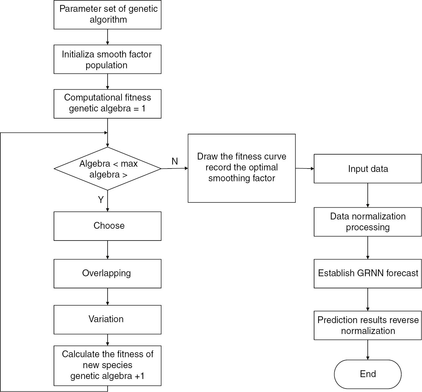
Genetic Improvement GRNN Method Forecasting Flowchart.
3.2 Genetic Improvement of Optimal Smoothing Factor
As for randomly generated smoothing factor groups, GA is conducted for screening based on fitness levels through selection, crossover, and mutation in inheritance. In this way, variables possessing the best fitness levels can be maintained, whereas those with low fitness levels will be omitted. New groups inherit information from the previous generation and supersede the previous ones in terms of performance.
This cycle is repeated until all conditions are met. GA consists of CODEC, individual fitness evaluation, and genetic operation. Genetic operation includes the selection, crossover, and mutation of chromosomes. Based on basic GA, this paper adopts the following technologies for optimization.
3.2.1 Encoding and Decoding
Encoding is the method for transferring feasible solutions of smoothing factors in solution space to identify the space that algorithms can handle.
Binary code not only conforms to the principles of computer information processing but also facilitates the crossover and mutation operations on chromosomes. The paper adopts the binary encoding method to search for randomly generated individuals within the prescribed scope. Each individual is given the value of smoothing factor σ. In crossover and mutation operations, binary values can be directly applied. As for the calculation of individual fitness values, binary values should be decoded to decimal values.
3.2.2 Fitness Evaluation
Fitness is used to measure the excellence degree of optimum values that smoothing factors may attain or get relatively close to. The method used to calculate individual fitness is called fitness function. This method is an evaluation function used in guiding the searching process in GA.
How to construct the fitness function is one of the most notable problems in GA. In this paper, the GRNN is established through fitness function. The adjacent five samples are selected and monitored. The target values of three samples adjacent to the previous five samples are predicted. The reciprocal of the Euclidean distance between the prediction results and the true value is used here as the fitness function.
The smaller the value of Euclidean distance is, the larger values form the fitness value. X is the true value and x is the prediction value. The fitness value is
3.2.3 Genetic Operation
3.2.3.1 Choice
The selection of determining crossover or mutation individuals.
The method used in this paper is for smoothing factor group S with the scale of N, based on the selective probability of xi∈S determined by each chromosome P(xi), randomly selected N chromosome from S.
The computational formula of selective probability is
Based on selective probability, randomly choose chromosomes and use the method of roulette wheel selection.
Generate a uniform distribution of random numbers in the (0,1) interval r. If r≤q1 is established, then chromosome x1 is selected. If qk−1<r<qk(2≤k≤N) is established, then chromosome xk is selected, where qi is the cumulative probability of chromosome xi(i=1, 2, …, N). The formula is
3.2.3.2 Overlapping
Crossing is the exchange of two genes that are selected from some of the genes on the chromosome, enabling new individuals to be generated through the combination of information from the parent.
3.2.3.3 Variation
Mutation is carried out to change certain genes in chromosomes (i.e. by changing 0 to 1 and 1 to 0). In fact, offspring genes change based on small disturbances.
The mutation process is similar to the crossover process. Based on preset mutation probability, whether or not to conduct a mutation operation should be decided. If conducted, a mutation position will be randomly produced. If not conducted, the mutation operation will not be activated.
3.3 Termination Principle of GA
The termination of GA involves several principles. For instance, when the largest artificial evolutionary algebra is reached, it should then accordingly be terminated. Another example is that when the fitness function value exceeds certain levels, it should similarly be terminated.
In this paper, GA predestinates the largest possible evolutionary algebra. Optimization will be terminated if the largest evolutionary algebra value is reached. GA also takes into consideration the overall fitness value changes of consecutive multiple generations. If the largest fitness value of consecutive multiple generations does not highlight obvious changes, and the average value of the fitness value for each generation remains close to the largest fitness value, then the process should be terminated and considered effective. Alternatively, GA should be performed again.
4 Example of Railway Freight Volume Forecast
To verify the effectiveness of theoretical algorithm, an algorithm program is compiled under the context of MATLAB (The MathWorks, Natick, MA, USA). Moreover, MATLAB neural network tools are used to establish two prediction models: genetically improved GRNN model and unimproved GRNN model.
4.1 Index System
There are many influencing factors of railway freight volumes. After calculating the degree of gray incidence, those influential factors with a degree of gray incidence of >0.6 to railway freight volumes should be selected.
Factors that mostly affect this are domestic products (100 million yuan), industrial products (100 million yuan), total coal production (million tons of standard coal, iron, and steel, including pig iron, crude steel, and steel production; 10,000 tons), crude oil output (10,000 tons), grain total output (10,000 tons), coke yield (10,000 tons), railway freight car ownership (cars), railway operating mileage (1 million km), double track railway (%), railway freight cargo volume share (%; a total of 11 elements all in all: I1–I11, respectively), and railway freight volume (10,000 tons) expressed by V.
As the 2014 statistical data have not yet been fully released, in addition to the 1990 data not being fully comprehensive, this paper selected the years 1990 to 2013 as its relevant data, all derived from the statistical yearbook of China (Table 1).
Railway Freight Volume and Its Influencing Factors in 1990 to 2013.
| Serial number | Year | V | I1 | I2 | I3 | I4 | I5 | I6 | I7 | I8 | I9 | I10 | I11 |
|---|---|---|---|---|---|---|---|---|---|---|---|---|---|
| 1 | 1990 | 150,681 | 18,667.8 | 6858.0 | 77,110.1 | 18,026.0 | 13,831.0 | 44,624.3 | 7328.0 | 364,966 | 5.79 | 24.4 | 15.52 |
| 2 | 1991 | 152,893 | 21,781.5 | 8087.1 | 77,689.4 | 19,503.0 | 14,099.0 | 43,529.3 | 7352.0 | 370,054 | 5.78 | 25.0 | 15.51 |
| 3 | 1992 | 157,627 | 26,923.5 | 10,284.5 | 79,691.2 | 22,380.0 | 14,210.0 | 44,265.8 | 7984.0 | 373,233 | 5.81 | 25.5 | 15.07 |
| 4 | 1993 | 162,794 | 35,333.9 | 14,188.0 | 82,183.7 | 25,411.0 | 14,524.0 | 45,648.8 | 9320.0 | 390,097 | 5.86 | 26.6 | 14.59 |
| 5 | 1994 | 163,216 | 48,197.9 | 19,480.7 | 88,571.8 | 27,430.0 | 14,608.0 | 44,510.1 | 11,477.0 | 415,919 | 5.90 | 28.7 | 13.83 |
| 6 | 1995 | 165,982 | 60,793.7 | 24,950.6 | 97,162.6 | 29,045.1 | 15,005.0 | 46,661.8 | 13,510.0 | 432,731 | 6.24 | 31.0 | 13.44 |
| 7 | 1996 | 171,024 | 71,176.6 | 29,447.6 | 99,774.0 | 30,184.6 | 15,733.4 | 50,453.5 | 13,643.0 | 443,893 | 6.49 | 32.5 | 13.17 |
| 8 | 1997 | 172,149 | 78,973.0 | 32,921.4 | 99,160.8 | 32,384.5 | 16,074.1 | 49,417.1 | 13,731.0 | 437,686 | 6.60 | 33.1 | 13.47 |
| 9 | 1998 | 164,309 | 84,402.3 | 34,018.4 | 95,168.3 | 34,160.5 | 16,100.0 | 51,229.5 | 12,806.0 | 439,326 | 6.64 | 34.2 | 12.96 |
| 10 | 1999 | 167,554 | 89,677.1 | 35,861.5 | 97,500.0 | 37,075.0 | 16,000.0 | 50,838.6 | 12,073.7 | 436,236 | 6.74 | 36.1 | 12.96 |
| 11 | 2000 | 178,581 | 99,214.6 | 40,033.6 | 98,855.1 | 39,097.5 | 16,300.0 | 46,217.5 | 12,184.0 | 439,943 | 6.87 | 36.5 | 13.14 |
| 12 | 2001 | 193,189 | 109,655.2 | 43,580.6 | 105,028.8 | 46,785.3 | 16,395.9 | 45,263.7 | 13,130.7 | 449,921 | 7.01 | 38.3 | 13.78 |
| 13 | 2002 | 204,956 | 120,332.7 | 47,431.3 | 110,732.2 | 54,572.8 | 16,700.0 | 45,705.8 | 14,279.8 | 446,707 | 7.19 | 38.7 | 13.82 |
| 14 | 2003 | 224,248 | 135,822.8 | 54,945.5 | 130,992.4 | 67,708.3 | 16,960.0 | 43,069.5 | 17,775.7 | 503,868 | 7.30 | 39.2 | 14.33 |
| 15 | 2004 | 249,017 | 159,878.3 | 65,210.0 | 151,615.6 | 87,097.8 | 17,587.3 | 46,946.9 | 20,619.0 | 520,101 | 7.44 | 39.1 | 14.59 |
| 16 | 2005 | 269,296 | 184,937.4 | 77,230.8 | 167,785.9 | 107,470.3 | 18,135.3 | 48,402.2 | 25,411.7 | 541,824 | 7.54 | 39.4 | 14.46 |
| 17 | 2006 | 288,224 | 216,314.4 | 91,310.9 | 180,625.9 | 130,053.4 | 18,476.6 | 49,804.2 | 29,768.3 | 558,483 | 7.71 | 39.8 | 14.15 |
| 18 | 2007 | 314,237 | 265,810.3 | 110,534.9 | 192,135.8 | 153,141.3 | 18,631.8 | 50,160.3 | 33,553.4 | 571,078 | 7.80 | 40.5 | 13.81 |
| 19 | 2008 | 330,354 | 314,045.4 | 130,260.2 | 200,103.9 | 158,590.5 | 19,043.1 | 52,870.9 | 32,031.5 | 584,961 | 7.97 | 41.6 | 12.78 |
| 20 | 2009 | 333,348 | 340,902.8 | 135,239.9 | 212,280.5 | 181,907.1 | 18,949.0 | 53,082.1 | 35,510.1 | 594,388 | 8.55 | 43.8 | 11.80 |
| 21 | 2010 | 364,271 | 401,512.8 | 160,722.2 | 227,437.7 | 203,732.9 | 20,241.4 | 54,647.7 | 38,864.0 | 622,284 | 9.12 | 44.8 | 11.24 |
| 22 | 2011 | 393,263 | 473,104.0 | 188,470.2 | 247,393.9 | 221,198.8 | 20,287.6 | 57,120.8 | 43,270.8 | 644,677 | 9.32 | 45.2 | 10.64 |
| 23 | 2012 | 390,438 | 519,470.1 | 199,670.7 | 253,863.7 | 234,320.5 | 20,571.1 | 58,958.0 | 44,778.9 | 664,333 | 9.76 | 46.2 | 9.52 |
| 24 | 2013 | 396,697 | 568,845.2 | 210,689.4 | 257,040.0 | 255,563.3 | 20,946.9 | 60,193.8 | 47,932.0 | 715,492 | 10.31 | 47.8 | 9.68 |
4.2 Data Processing
In the prediction process, in most cases, the prediction of incremental data can produce better output effects than do the direct prediction of data. To establish the actual railway freight volume, the improved algorithm is used to forecast the data increment. According to the actual situation of railway freight volume, the improved algorithm is used to forecast the data increment.
Using I1 to I11 and V values from years 1991 to 2013 minus the relevant values from last year, respectively, incremental data I1 to I11 and V are obtained for the 23 years. The paper conducts an input and forecasting on the aforementioned incremental data. The incremental data of 9 consecutive years should be placed in a group. The former 8 years of data will be used in the optimization of smoothing factor and GRNN training. The ninth year data will be used in the forecast.
In this way, the incremental data are divided into 15 groups to predict the 1999 to 2013 railway freight increment. To prevent an increase in network training time caused by outlier sample data, normalization processing should conducted on various data (i.e. convert data to numerical values between 0 and 1).
In Eq. (4), the normalized value x′, as the original value xi, affects the same element xi in the minimum value xmin and affects the same element value xi of the maximum value xmax. After obtaining the predictive value, the range is between 0 and 1; therefore, the predicted value y′ should be reduced to the actual value by Eq. (5).
For the normalized value, the minimum value ymin of the network is the direct output value and the maximum value ymax of the network is the output value.
4.3 Forecasting Process
Using the GA optimization smoothing factor, the operating parameters are set as smoothing factor σ range of [0.05,1], precision arithmetic of 0.0001, population size of 50, biggest genetic algebra of 12, crossover probability of 0.9, and mutation probability of 0.09.
In terms of fitness function, the incremental data of each group of the first 8 years are divided into two parts: the first part relates to the first 5 years and the second part for the last 3 years. The first part of training GRNN is thus used to predict the second part of the freight increment value.
When using the GA optimization smoothing factor, operating parameters are set as follows: the population size is the number of individuals, and as the size is too large, GAs will actually become exhaustive enumeration to search for the best, which means that it is impossible to add all the possible solutions of the corresponding individual to form a population.
For setting the population size, not only the quality of the optimization, an individual factor to obtain the optimal smoothing factor, should be taken into account but also the time to get the optimal value, the calculation speed of optimization, should be considered. “Fast and good” is the overall goal of the algorithm. If the population size is too small, “congenitally deficient” with a large number of variable genotypes deletion will be born in the initial population, with the great reducing probability of having a better individual, slow population evolutionary rate, and being easy to fall into local optimal solution; thus, the worse overall optimization results come into being. However, if the population size is large, the calculated amount to calculate the fitness of all individuals and do genetic operations will be great, which makes the calculation time too long and the searching speed slower.
Based on the above analysis, in consideration of the acceptability of computational time, we should increase the population size as much as possible. In this paper, all individuals in the initial smoothing factor group are randomly generated, and the population size is set as 50. The arithmetic precision is set as 0.0001, and the range of the smoothing factor is [0.05,1]. Then, we can obtain that the bit length is equal to ceil [log2(1−0.05)/0.0001], that is, 14.
Through complementary advantages, we make the chosen two individuals who have been highly adaptive become more excellent individuals, that is, intersection. The higher the crossover frequency is, the more complete recombination of good genes can be obtained and the faster the optimal solution is reached. However, if the crossover probability is too high, the population may become unstable, and the individuals who have been very close to the optimal solution are easy to be destroyed and become “transient”, which reduces the evolutionary efficiency on the contrary. The cross-probability in this paper is set as 0.9. The evolution generation is the number of cycles that constantly produce new generations of individuals. In general, more frequent evolution leads to better solutions. However, with too many evolution generations, the computation times will increase and the computation processing time is longer. Therefore, after certain generations, the solution represented by the optimal individual may be convergent. In this paper, the maximum genetic evolution generation is set as 12.
4.4 Forecast Results
Observations are made of the biggest fitness curve and average fitness curve in genetic arithmetic. No large-scale vibrations are evident. Algorithm convergence progressed smoothly. In the evolution process, two curves showed a similar tendency, and the maximum adaptation of individual successive generations did not evolve, suggesting that populations are mature.
Curve graphs are selected as shown in Figures 2–5. Other years have similar predictions. It does not need to be repeated here.
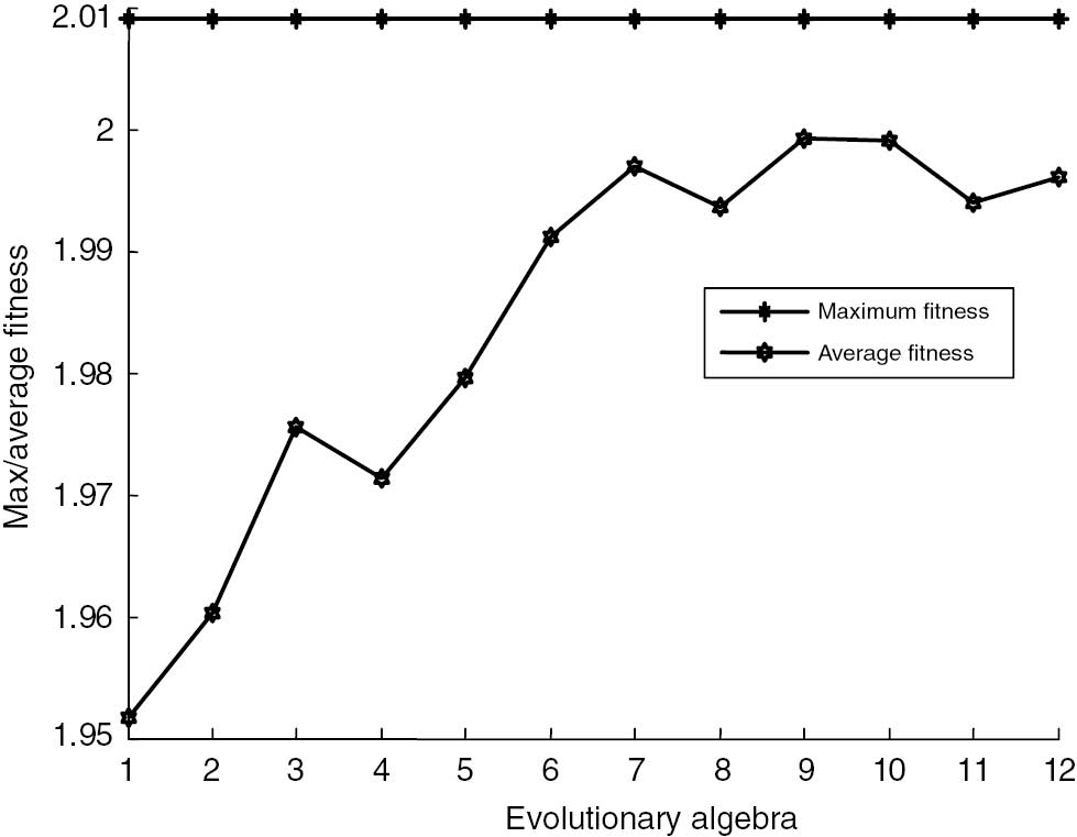
Smoothing Factor Fitness Curve of Railway Freight Increment in 2006.
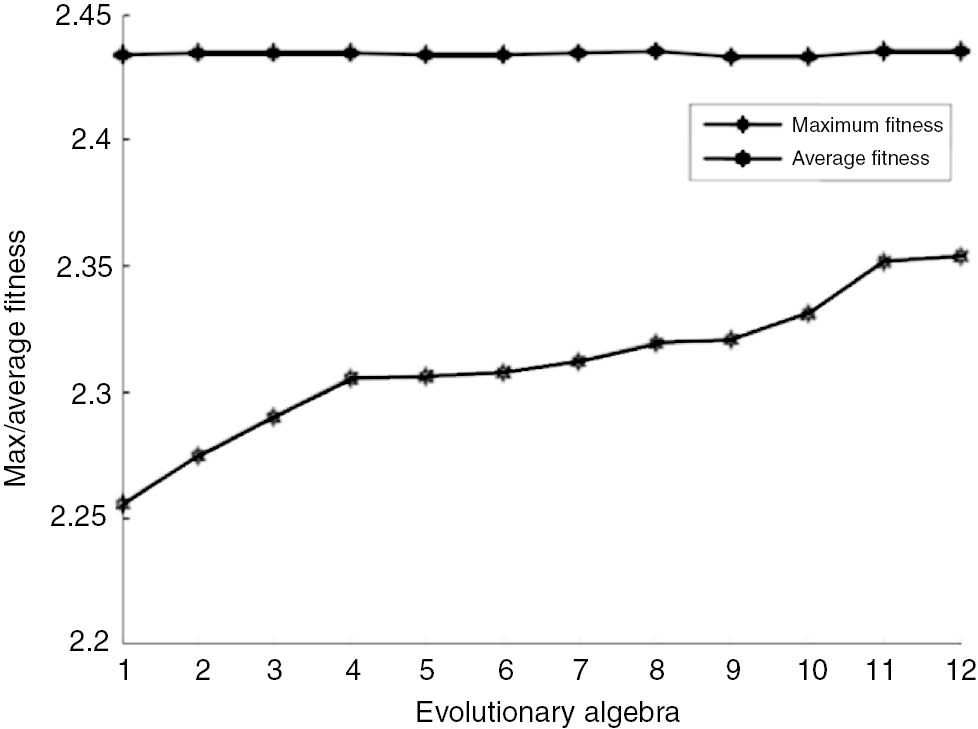
Smoothing Factor Fitness Curve of Railway Freight Increment in 2007.
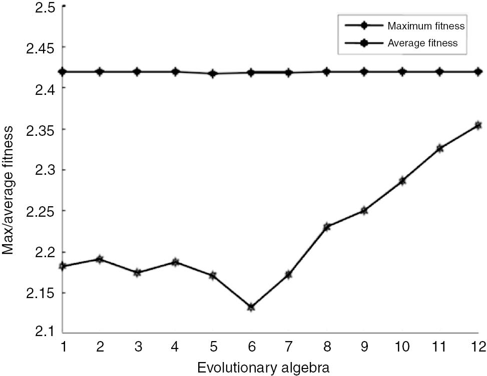
Smoothing Factor Fitness Curve of Railway Freight Increment in 2009.
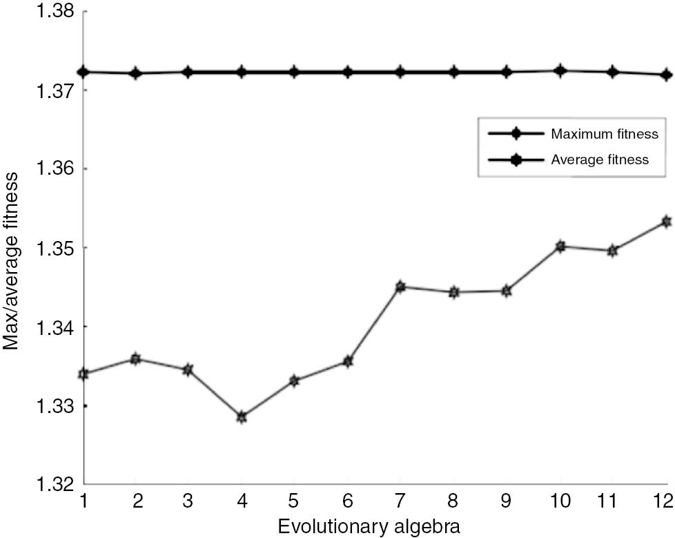
Smoothing Factor Fitness Curve of Railway Freight Increment in 2010.
The GA, the respective smoothing factor by the GRNN, and the prediction results are obtained for the railway freight increment. The actual freight volume of the year before the year of the incremental forecasting results can be predicted by the railway freight volume as shown in Table 2.
Prediction Results of the GRNN and Genetic Improvement in the GRNN.
| Year | Volume of freight traffic | Smoothing factor σ | Prediction results | Absolute value of percentage error | |||
|---|---|---|---|---|---|---|---|
| GRNN | Genetic improvement GRNN | GRNN | Genetic improvement GRNN | GRNN (%) | Genetic improvement GRNN (%) | ||
| 1999 | 167,554 | 0.1 | 0.41712 | 164,310 | 165,195 | 1.94 | 1.41 |
| 2000 | 178,581 | 0.1 | 0.99942 | 167,550 | 169,627.9 | 6.18 | 5.01 |
| 2001 | 193,189 | 0.1 | 0.095404 | 178,581 | 183,748 | 7.56 | 4.89 |
| 2002 | 204,956 | 0.1 | 0.99577 | 193,189 | 199,882.4 | 5.74 | 2.48 |
| 2003 | 224,248 | 0.1 | 0.67724 | 204,956 | 217,000 | 8.6 | 3.23 |
| 2004 | 249,017 | 0.1 | 0.42477 | 224,248 | 242,987 | 9.95 | 2.42 |
| 2005 | 269,296 | 0.1 | 0.21694 | 249,017 | 273,786 | 7.53 | 1.67 |
| 2006 | 288,224 | 0.1 | 0.063511 | 269,296 | 289,575 | 6.57 | 0.47 |
| 2007 | 314,237 | 0.1 | 0.41828 | 288,224 | 308,047 | 8.28 | 1.97 |
| 2008 | 330,354 | 0.1 | 0.69742 | 314,237 | 333,277 | 4.88 | 0.88 |
| 2009 | 333,348 | 0.1 | 0.7528 | 330,354 | 349,612 | 0.9 | 4.88 |
| 2010 | 364,271 | 0.1 | 0.75077 | 333,348 | 353,300 | 8.49 | 3.01 |
| 2011 | 393,263 | 0.1 | 0.068266 | 364,271 | 390,284 | 7.37 | 0.76 |
| 2012 | 390,438 | 0.1 | 0.10973 | 393,263 | 409,380 | 0.72 | 4.85 |
| 2013 | 396,697 | 0.1 | 0.58754 | 390,438 | 405,699 | 1.58 | 2.27 |
| Average | 5.75 | 2.68 | |||||
The curve convergence in recent years has been more pronounced. The fitness curve is obtained by predicting freight increments of other years; either the average fitness curve rose slightly slow, similar to Figure 3, or the average fitness curve decreased first and then increased, similar to Figure 4, but the maximum fitness curve in the evolutionary process of 12 generations is always in a horizontal line, which can also be considered that the population has been mature, reaching the aim of the individual optimization of smoothing factor.
Population maturity means that the best individuals, that is, the best smoothing factor, occurs in the population. The best individual is the smoothing factor that gets the maximum fitness. Even if the theoretical best individual values do not occur in the population, the individual values that appear to have the maximum fitness value are approximately equal to the theoretical best individual values. After all, the probability that a GA can get an exact optimal value is less than 1; unless the evolution generation is infinite, the probability can reach 1. But in fact, after two or three evolutions, individuals who are approximately equal to the theoretical optimum will occur.
As the average GRNN uses a fitting degree of training samples to determine the smoothing factor within the range from 0.1 to 0.5, the average GRNN smoothing factor often reaches the value of 0.1. Moreover, in the year of prediction, when the actual value of the GRNN is almost equal to that of last year, prediction accuracy is relatively high. When they are not almost equal to each other, prediction accuracy is relatively low. In the 15 years of prediction, the absolute value relative error of the genetically improved GRNN only accounts for 5.01% of the whole year. The rest of the absolute value relative errors are all below the level of 5%. In addition, when the average value of the absolute value relative errors is lower than 3%, prediction accuracy is relatively enhanced.
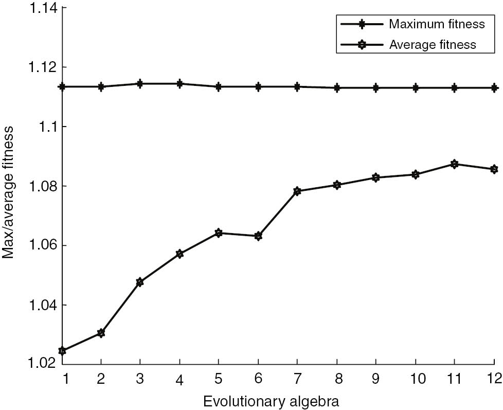
2015 Smoothing Factor of Railway Freight: Incremental Fitness Curve Prediction.
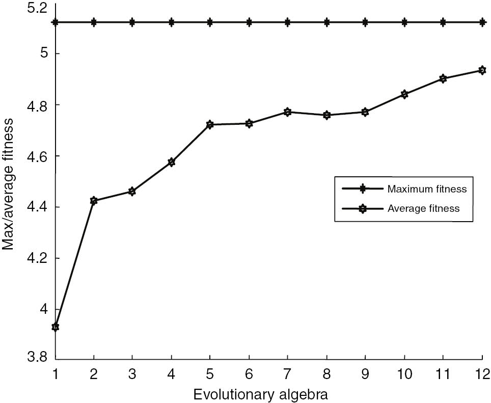
2016 Smoothing Factor of Railway Freight: Incremental Fitness Curve Prediction.
4.4.1 Extended Forecast
In this paper, a new method of genetic improvement based on the GRNN is proposed and applied to railway freight volume forecasting. However, in general situations, it will take some time to obtain the statistical data of these 11 influencing factors. This would impact the promptness of predicting railway freight volumes, thus reducing the significance of prediction results.
The solution is to consider real-time supervision to obtain statistical data of relevant influencing factors. Other suitable prediction methods can also be adopted to predict the values of 11 influencing factors. Moreover, the prediction values of these influencing factors can be regarded as the input value, and then the prediction of railway freight volumes can be conducted.
As most influencing factors of railway freight volumes indicate stability, few change or show certain obvious tendencies, such as gross domestic product. Based on the development of the national economy, and macroeconomic regulation and control, increases are achieved between 6% and 8%. Thus, the method of exponential smoothing can be used to predict the 11 influencing factors. Then, the prediction value of the influencing factors can be substituted into the improved algorithm to obtain the forecast value of railway freight volumes.
Such a way of prediction – data obtained through traditional prediction methods before using the improved algorithm – is used to obtain the desired final prediction result, which is also scientific, because while using the influencing factors to predict railway freight volumes the influencing factors have nonlinear relations with target values. Moreover, it is in conformity with the mathematical model set by the traditional prediction method.
As for the prediction of the influencing factors, based on the above analysis, it is suitable for the traditional prediction method. In other words, as for the prediction of different target values, different suitable prediction methods should be adopted to fit different target values.
Based on the scientific and reasonable target prediction values obtained by the traditional prediction method, it is reasonable to select these prediction results and regard them as the influencing factors, because the next prediction process is not related to the prediction results of the previous one, as long as the previous prediction results are scientific, reasonable, and reliable.
Based on the above analysis, forecasting is conducted on railway freight volumes in 2015 and 2016. Considering that Chinese economic growth has entered the new normal state, and the overall international economic development has slowed down, while using SPSS software to predict the influencing factors, the method of exponential smoothing is adopted. The prediction values of railway freight volume influencing factors from 2014 to 2016 are shown in Table 3.
Influence Factors of Railway Freight Volume in 2014 to 2016.
| Year | I1 | I2 | I3 | I4 | I5 | I6 | I7 | I8 | I9 | I10 | I11 |
|---|---|---|---|---|---|---|---|---|---|---|---|
| 2014 | 619,666.9 | 225,525.2 | 259,892.8 | 273,348.6 | 21,226.9 | 60,717.3 | 50,490.1 | 740,316 | 10.78 | 48.7 | 9.29 |
| 2015 | 670,485.1 | 240,360.2 | 262,455 | 291,674.5 | 21,526.7 | 61,240.6 | 52,908.9 | 765,139 | 11.25 | 49.7 | 9.13 |
| 2016 | 721,300 | 255,194.9 | 264,756.3 | 309,982 | 21,826.4 | 61,763.5 | 55,195.4 | 789,963 | 11.71 | 50.6 | 9.01 |
In 2015 and 2016, the smoothing factor fitness curve of the railway freight increment is predicted as shown in Figures 6 and 7.
GA was used to predict the 2015 and 2016 railway freight incremental GRNN smoothing factor σ, and the smoothing factor σ was substituted into the GRNN. The rail freight incremental predictive results are shown in Table 4.
Railway Freight Volume Forecasting in 2015 and 2016.
| Year | Smoothing factor σ | Railway freight increment prediction results | Railway freight increment prediction results |
|---|---|---|---|
| 2015 | 0.93685 | 11,633 | 392,967 |
| 2016 | 0.81694 | 8942.3 | 401,909.3 |
From the website of the National Bureau of Statistics, it can be learned that in 2014 the railway freight volume reached 3.81334 billion tons. Then, the railway freight volumes of 2015 and 2016 can be obtained through relevant calculations.
5 Conclusion
The accurate prediction of railway freight volume is of great importance in railway planning, construction, and operation decision. In this study, a creative genetic improvement of the railway freight volume forecasting method of the GRNN is proposed. Meanwhile, by writing the MATLAB code and applying the MATLAB neural network toolbox method to verify its validity, this study finds out that the improved algorithm can effectively reduce the prediction error, demonstrating its obvious superiority.
In this paper, a new method of genetic improvement based on the GRNN is proposed, and it is applied to railway freight volume forecasting.
Compared to the former method, GA is more highly effective because it takes into consideration the subjective factors. The prediction results show that using the same number of training samples, and forecasting the same target, the genetic improvement of the GRNN model prediction accuracy is better in predicting target values and therefore indicates a large improvement in forecasting accuracy.
The set of improved algorithm to calculate fitness function forms an innovative method using a “5+3” mode, namely, to establish a GRNN, with the continuous five training samples, capable of predicting the next five samples. The predicted results and the real value of the reciprocal of the Euclidean distance as the fitness function ensure a smoothing factor optimization that can be used to forecast any change in trend of the target data.
Finally, a forecast of incremental data is calculated, rather than using direct projections of the data, and then the prediction results are calculated. It is concluded that this system is suitable to forecast the target. Furthermore, this method of data processing makes forecasting more sensitive as well as brings prediction results closer to their real value. The combination model based on the genetic modified generalized neural network has greatly improved the accuracy of predicting railway freight volume, which provides a reference of forecasting the freight volume in railway transportation production. However, due to the complexity of the research subject, it is still necessary to conduct studies for improvement. The application of the MATLAB neural network toolbox creates a GRNN, in which the same smoothing factor can be used for all model layer basis functions. Therefore, as long as the one-dimensional smoothing factor is optimized, the process of the GA can be completed. If we choose to establish the GRNN by programming the source program rather than the neural network toolbox, there will be different values for the smoothing factor. The smoothing factor can be set as a series of numbers for conducting a multidimensional optimization on smoothing factor. The result will be applied to establish a GRNN to predict errors, which can further lower the possibility of error.
Acknowledgments
This work was supported by the Guidance Project of the Liaoning Natural Science Foundation (project number 20170540124) and the Science Research Project of the Liaoning Provincial Department of Education (project number JDL2016032). The authors wish to acknowledge the support and efforts of all authors who were involved in this paper and particularly express their sincere gratitude to all those who have helped improving the content and format of the paper.
Bibliography
[1] M. W. Babcock, X. Lu and J. Norton, Time series forecasting of quarterly railroad grain car loadings, Transport. Res. Pt. E35 (1999), 43–57.10.1016/S1366-5545(98)00024-6Search in Google Scholar
[2] P. J. Brockweil and R. A. Davis, Time series: theory and methods, Springer-Verlag, New York, NY, 1991.10.1007/978-1-4419-0320-4Search in Google Scholar
[3] L. Y. Geng, T. W. Zhang and P. Zhao, Forecast of railway freight volumes based on LS-SVM with grey correlation analysis, J. China Railw. Soc.34 (2012), 1–6.Search in Google Scholar
[4] G. A. Godfrey and W. B. Powell, Adaptive estimation of daily demands with complex calendar effects for freight transportation, Transport. Res. Pt. B34 (2000), 451–469.10.1016/S0965-8564(99)00032-4Search in Google Scholar
[5] Y. H. Guo, Z. Y. Chen, F. L. Feng and B. Chang, Railway freight volume forecasting of neural network based on economic cycles, J. China Railw. Soc.32 (2010), 1–6.Search in Google Scholar
[6] W. U. Huawen and W. Fuzhang, Research on railway freight traffic prediction based on maximum lyapunov exponent, J. China Railw. Soc.36 (2014) 7–13.Search in Google Scholar
[7] H. Q. Li and K. Liu, Analysis of railway freight volume based on fractal theory, J. China Railw. Soc.25 (2003), 19–23.Search in Google Scholar
[8] H. Q. Li and K. Liu, Prediction of railway freight volumes based on rough set theory, J. China Railw. Soc.26 (2004), 1–7.Search in Google Scholar
[9] X. Y. Lin and Y. X. Chen, Study on railway freight volume forecast by the Gray-Markov chain method, J. China Railw. Soc.27 (2005), 15–19.Search in Google Scholar
[10] Z. J. Liu, L. Ji, Y. L. Ye and Z. M. Geng, Study on prediction of railway freight volumes based on RBF neural network, J. China Railw. Soc.28 (2006), 1–5.Search in Google Scholar
[11] T. L. Seng, M. Khalid and R. Yusof, Adaptive GRNN for the modeling of dynamic plants, in: IEEE International Symposium on Intelligent Control, Vancouver, Canada, vol. 10, pp. 217–222, 2002.10.1109/ISIC.2002.1157765Search in Google Scholar
[12] D. F. Specht, A general regression neural network, IEEE Trans. Neural Netw.2 (1991), 568–576.10.1109/72.97934Search in Google Scholar PubMed
[13] A. N. Yonge, B. Xueying and W. Qicai, Railway freight volume forecasting based on unbiased grey Verhulst model, J. China Railw. Soc.13 (2016), 181–186.Search in Google Scholar
[14] C. Zhang and X. F. Zhou, Prediction of railway freight volumes based on Gray forecast-Markov chain-qualitative analysis, J. China Railw. Soc.29 (2007), 15–21.Search in Google Scholar
[15] C. Zhao, K. Liu and D. S. Li, A study of use support vector machine theory of prediction freight volume, J. China Railw. Soc.26 (2004), 10–14.Search in Google Scholar
[16] C. Zhao, K. Liu and D. S. Li, Freight volume forecast based on GRNN, J. China Railw. Soc.26 (2004), 12–15.Search in Google Scholar
©2019 Walter de Gruyter GmbH, Berlin/Boston
This article is distributed under the terms of the Creative Commons Attribution Non-Commercial License, which permits unrestricted non-commercial use, distribution, and reproduction in any medium, provided the original work is properly cited.