Performance and Stability Bounds for Dynamic Networks ⋆ Dimitrios Koukopoulos ∗ Research and Academic Computer Technology Institute, P. O. Box 1122, 261 10 Patras, Greece. Marios Mavronicolas Department of Computer Science, University of Cyprus, 1678 Nicosia, Cyprus. Paul Spirakis Department of Computer Engineering and Informatics, University of Patras, Rion, 265 00 Patras, Greece & Research and Academic Computer Technology Institute, P. O. Box 1122, 261 10 Patras, Greece. ⋆ Submitted as a Regular Paper. A preliminary version of this work has been appeared in the Proceedings of the 7th International Symposium on Parallel Architectures, Algorithms and Networks, Hong-Kong, SAR, China, 2004, pp. 239–246. This work has been partially supported by the IST Program of the European Union under contract number IST-2001-33116 (FLAGS), by the 6th Framework Programme of the European Union under contract number 001907 (DELIS), and by funds for the promotion of research at University of Cyprus. ∗ Corresponding author. Telephone: +302641034473, Fax:+302641058075. Email addresses: koukopou@ceid.upatras.gr (Dimitrios Koukopoulos), mavronic@ucy.ac.cy (Marios Mavronicolas), spirakis@cti.gr (Paul Spirakis). Preprint submitted to Elsevier Science 28 January 2005 Abstract In this work, we study the impact of dynamically changing link capacities on the delay bounds of LIS (Longest-In-System) and SIS (Shortest-In-System) protocols on specific networks (that can be modelled as Directed Acyclic Graphs-DAGs) and stability bounds of greedy contention-resolution protocols running on arbitrary networks under the Adversarial Queueing Theory. Especially, we consider the model of dynamic capacities, where each link capacity may take on integer values from [1, C] with C > 1, under a (w, ρ)-adversary. We show that the packet delay on DAGS for LIS is upper bounded by O(iwρC) and lower bounded by Ω(iwρC) where i is the level of a node in a DAG (the length of the longest path leading to node v when nodes are ordered by the topological order induced by the graph). In a similar way, we show that the performance of SIS on DAGs is lower bounded by Ω(iwρC). We prove that every queueing network running a greedy contention-resolution protocol is stable for a rate not exceeding a particular stability threshold, depending on C and the length of the longest path in the network. Key words: Parallel Computing; Networks; Delay Bounds; Stability Bounds; Adversarial Queueing Theory 2 1 Introduction 1.1 Motivation-Framework We are interested in the behavior of packet-switched networks in which packets arrive dynamically at the nodes and they are routed in discrete time steps across the links. Recent years have witnessed a vast amount of work on analyzing packet-switched networks under non-probabilistic assumptions (rather than stochastic ones); We work within a model of worst-case continuous packet arrivals, originally proposed by Borodin et al. [5] and termed Adversarial Queueing Theory to reflect the assumption of an adversarial way of packet generation and path determination. A major issue that arises in such a setting is that of stability– will the number of packets in the network remain bounded at all times? Besides the existence or not of upper bounds on the packet delays (queue sizes), a complementary question concerning stability is whether stability guarantees that there are small bounds on packet delays (queue sizes). The answer to these questions may depend on the rate of injecting packets into the network, the capacity of the links, which is the rate at which a link forwards outgoing packets, and the protocol that is used to resolve the conflict when more than one packet wants to cross a given link in a single time step. The underlying goal of our study is two-fold. First, we want to estimate how good can be the performance bounds on packet delay (queue size) on DAGs and second we want to establish stability properties of greedy protocols. We study these problems considering that packets are injected by an adversary (rather than by an oblivious randomized process) and capacities are chosen by the same adversary in a dynamic way. Most studies of packet-switched networks assume that one packet can cross a network link (an edge) in a single time step. This assumption is well motivated when we assume that all network links are identical. However, a packetswitched network can contain different types of links, which is common especially in large-scale networks like Internet. Then, it is well motivated to assign a capacity to each link that takes on values from the integer set [1, C] with C > 1. If C is a large integer, we can consider approximately as a link failure the assigning of unit capacity to a link, and the assigning of capacity C as the proper service rate. Therefore, the study of protocol stability under this model of dynamically changing capacities can be considered as an approximation of the fault-tolerance of a network where links can temporarily fail (zero capacity). In this work we consider the impact on performance bounds and stability properties if the adversary besides the packet injections in paths which it 3 determines, it also can set the capacities of network edges in each time step. This subfield of study was initiated by Borodin et al. in [6]. Note that we continue to assume uniform packet sizes. Furthermore, we consider greedy contention-resolution protocols (all of which enjoy simple implementations)always advance a packet across a queue (but one packet at each discrete time step) whenever there resides at least one packet in the queue, such as LIS (Longest-in-System) that gives priority to the packets that have been for the longest amount of time in the network and SIS (Shortest-in-System) that gives priority to the packets that have been for the shortest amount of time in the network. Roughly speaking a protocol P is stable [5] on a network G against an adversary A of rate r if there is an integer B (which may depend on G and A) such that the number of packets in the system is bounded at all times by B. Moreover, a network G is universally stable [5] if every greedy protocol is stable against every adversary of rate less than 1 on G. Directed Acyclic Graphs (DAGs) are universally stable in the more powerful model of general dynamic capacities– each is stable against every adversary of rate less than 1 for every protocol [6, Theorem 3]. 1.2 Contribution We use here the model of dynamic capacities that has been initiated in [6] where link capacities may take on integer values in the interval [1, C] with C > 1 1 under a (w, ρ)-adversary that injects packets at rate ρ with window size w. In this framework, we obtain the following results: • The delay of packets on DAGs (where the LIS protocol is running on top of them) is upper bounded by O(iwCρ) where i is the level of a node on a DAG (the length of the longest path leading to node v when nodes are ordered by the topological order induced by the graph). We use double-induction on time and the node level to prove it. • We make this performance bound tight showing a lower bound of Ω(iwCρ) on the packet delay that is suffered by a packet targeted with a node u of level i. The maximum queue size in this case is (w + 1)C. The proof of this result is based on an involved adversarial construction. Also, it considers the weakest dynamic model where a link capacity can take on values from the two-valued set of integers 1 and C. Thus, the tight bound we prove here imply the collapse of a powerful model to a weaker one that is rather surprising. In a similar way, we prove that the SIS protocol has a lower bound of Ω(iwCρ) on the packet delay when it is running on top of DAGs. 1 The classical Adversarial Queueing Theory corresponds to the case where only one capacity value is available to the adversary. 4 • We show two simple results which provide some upper bounds on the allowable rate of injections that still guarantees stability. Specifically, we prove that any arbitrary network running a greedy contention-resolution protocol 1 , where d(G) is stable as long as the injection rate does not exceed C(d(G)+1) is the length of the longest path in the network that can be followed by any packet. A slightly improved result is proved for the stability threshold in the case of a special class of greedy protocols, the time priority protocols. Such a protocol is stable on all networks as long as the injection rate of the 1 . adversary does not exceed Cd(G) Roughly speaking, the results that have been obtained in this paper show that the linear performance bounds that have been proved in the classical setting of Adversarial Queueing Theory remain linear when link capacities vary dynamically although the adversary in such environments is more powerful. The only difference is that the performance bounds in the dynamic setting have as expense a multiplicative factor of C. The same holds for the stability thresholds that are obtained in this paper for dynamically varying link capacities. 1.3 Related Work Stability Issues under the Adversarial Queueing Model. Adversarial Queueing Theory was developed by Borodin et al. [5] as a more realistic model that replaces traditional stochastic assumptions in Queueing Theory by more robust, worst-case ones. Adversarial queueing theory received a lot of interest in the study of stability and instability issues (see, e.g., [2,8,9,12,13]). The universal stability of various natural greedy protocols (LIS, SIS, NTS (Nearest-to-Source), FTG (Furthest-to-Go) has been established by Andrews et al. [2]. Furthermore, the set of universally stable networks has been wellcharacterized [2,5] (DAGs, trees, ring). Stability Bounds for Greedy Protocols. The subfield of proving stability thresholds for greedy protocols on every network was first initiated by Diaz et al. [8] showing an upper bound on injection rate for the stability of FIFO in networks with a finite number of queues that is based on network parameters. This result was significantly improved for all networks by Koukopoulos et al. [10] demonstrating a method for estimating an upper bound for FIFO stability which is, also, based on network parameters. In an alternative interesting work, Lotker et al. [13] proved that any greedy protocol can be stable in any network if the injection rate of the adversary is upper bounded by 1/(d + 1), where d is the maximum path length that can be followed by any packet. Also, they proved that for a specific class of greedy protocols, time-priority protocols, the stability threshold becomes 1/d. In the subfield of proving instability thresholds for greedy protocols (lower bound on injection rate that guarantees instability), 5 Bhattacharjee and Goel [4] proved that FIFO can become unstable for arbitrarily small injection rates on parameterized network constructions under the adversarial queueing theory model. Performance Bounds for Greedy Protocols. Several universally stable protocols have exponential lower bounds on queue sizes and packet delays (SIS, NTS, FTG) [2]. Andrews and Zhang [3] proved that LIS has an exponential lower bound on packet delay on a tree with exponential depth in the length of the longest network path. Scheideler and Vöcking [14] proved that a protocol in the spirit of LIS with additional control packets using queues of constant size suffers from linear packet delay on layered graphs under a close related model to the Adversarial Queueing Model. In an interesting work, Adler and Rosén [1] proved tight polynomial bounds for the stability of LIS on DAGs. Especially, they have shown that LIS on DAGs has linear (in the longest path in the network that can be followed by any packet) queue sizes and packet delays. Stability Issues in Dynamic Networks. Borodin et al. in [6] studied for the first time the impact on stability when the network links can have capacities. They proved that many well-known universally stable protocols (SIS, NTS, FTG) do maintain their universal stability when the link capacity is changing dynamically, whereas the universal stability of LIS is not preserved. Also, the universal stability of networks is preserved under this varying context. The study of stability properties of protocols and networks when link capacities change dynamically has been further extended in [11] presenting involved combinatorial constructions of the adversary that lead LIS and certain √ compositions of universally stable protocols to instability for a threshold of 2 − 1, while all the known forbidden subgraphs for the universal stability of networks are proved to have lower instability thresholds. 1.4 Road Map The rest of this paper is organized as follows. Section 2 presents our model definitions. Bounds for the LIS protocol on DAGs are presented in Section 3. A bound for the SIS protocol on DAGs is presented in Section 4. Section 5 includes our upper bounds on the stability threshold of any network. We conclude, in Section 6, with a discussion of our results and some open problems. 6 2 Model The model definitions are patterned after those in [5, Section 3], adjusted to reflect the fact that link capacities may vary arbitrarily as in [6, Section 2] (link capacities may take on integer values in the interval [1, C] with C > 1). Along with this model, we address the weakest possible model of changing capacities in which link capacity can take on a value from a two-valued set of integers {1, C} with C > 1. A routing network is modelled as a directed graph G =(V, E) with |V | = n nodes and |E| = m edges. Each node v ∈ V represents a communication switch and each directed edge e ∈ E represents a link between two switches that delivers packets only in the direction it is oriented. Every switch has a buffer (queue) at the tail of each out-going link and stores there the packets to be sent on the corresponding link. Time proceeds in discrete steps. New packets, requiring to traverse predetermined paths, can be injected into the network at any time step. A packet is an atomic entity that resides at a node at the end of any step. It must travel along paths in the network from its source to its destination, both of which are nodes in the network. When it reaches its destination, we say that it is absorbed. During each step, a packet may be sent from its current node along one of the outgoing edges from that node. Edges can have different integer capacities, which may or may not vary over time. Denote Ce (t) the capacity of edge e at time step t. That is, we assume that edge e is capable of simultaneously transmitting up to Ce (t) packets at time t. Any packets that wish to travel along an edge e at a particular time step, but they are not sent, wait in a queue for edge e. The delay of a packet is the number of steps that are spent by the packet, while waiting in queues. At each step, an adversary generates a set of requests. A request is a path specifying the route that will be followed by a packet. 2 We say that the adversary generates a set of packets when it generates a set of requested paths. We restrict our study to the case of non-adaptive routing, where the path traversed by each packet is fixed at the time of injection, so that we are able to focus on queueing rather than routing aspects of the problem. There are no computational restrictions on how the adversary chooses its requests in any given time step. Fix any arbitrary positive integer w ≥ 1. Throughout, for any sequence of time steps T = [t1 , t2 ] and for any integer w ≥ 1, denote T ± w the sequence of time steps [t1 − w, t2 + w]. For any edge e of the network and any sequence Tw of w consecutive time steps, define N (T , e) to be the number of paths that are injected by the adversary during the time interval T requiring to traverse the edge e. For any constant ρ, 0 < ρ ≤ 1, a (w, ρ)-adversary Aw,ρ is an adversary 2 In this work, it is assumed, as it is common in packet routing, that all such paths are simple paths with no overlapping edges. 7 that injects packets subject to the following load condition: For every edge e and for every sequence Tw of w consecutive time steps, N (Tw , e) ≤ ρ  C(τ ) . τ ∈Tw We say that a (w, ρ)-adversary Aw,ρ injects packets at rate ρ with window size w. Lemma 2.1 Fix any (w, ρ)-adversary Aw,ρ . Then, for any time step t ≥ 1 and for any edge e, N ([t], e) ≤ ρ max max{1,t−w+1}≤δ≤t  C(τ ) . δ≤τ ≤δ+w−1 Lemma 2.1 immediately implies: Corollary 2.2 Fix any (w, ρ)-adversary Aw,ρ . Then, for any edge e, N ([1], e) ≤ ρ  C(τ ) . 1≤τ ≤w Lemma 2.3 Fix any (w, ρ)-adversary Aw,ρ . Then, for any time interval T and for any edge e, N (T , e) ≤ ρ  C(τ ) . τ ∈T ±w The assumption that ρ ≤ 1 ensures that it is not necessary a priori that some edge of the network is congested (which would surely happen when ρ > 1). A contention-resolution protocol specifies, for each pair of an edge e and a time step, which packet among those waiting at the tail of edge e will be moved along edge e. A greedy contention-resolution protocol always specifies some packet to move along edge e if there are packets waiting to use edge e. In this work, we restrict attention to deterministic, greedy contention-resolution protocols, such as LIS (Longest-in-System) where priority is given to the packets that have been for the longest amount of time in the network. All these contention-resolution protocols require some tie-breaking rule in order to be unambiguously defined. In this work, whenever we are proving a positive result, we assume that the adversary can break the tie arbitrarily; for proving a negative result, we can assume any well-determined tie breaking rule for the adversary. 8 We continue with some additional formal definitions that are needed to make the discussion more precise. Formally, a packet p is a triple id, π, t0 , where id is some unique identifier, π is the path (from the origin to the destination of the packet), and t0 is the time when the packet is injected into the network (at its origin node). The state of a packet p at time t, denoted state t (p), is the tuple p, δ, t1 , . . . , tδ , where δ is the number of time steps at which p has traversed an edge in its path, and t1 , . . . , tδ are the corresponding times of such traversals. For simplicity, and in a way similar to that in [2] and in works following it, we omit floors and ceilings from our analysis, and we sometimes count time steps and packets only roughly. This may only result to loosing small additive constants, while it implies a gain in clarity. 3 LIS on Directed Acyclic Graphs Upper and lower bounds on the performance of LIS on directed acyclic graphs appear in Sections 3.1 and 3.2, respectively. Throughout this section, we will consider directed acyclic graphs, in which nodes are ordered by the topological order induced by the graph. This order assigns to each node v a level i ≥ 0, denoted level (v), such that the longest path leading to node v has length i. 3.1 Upper Bound In this section, we present our upper bound on the performance of LIS on directed acyclic graphs. We start by proving: Proposition 3.1 Consider any packet p that is injected at time t, and let v be any node of level i ≥ 0 on its path other than its destination node. Then, packet p clears node v by time t + δ(t), where δ(t) > 0 is the least integer such that  t≤τ ≤t+δ(t) C(τ ) ≥ ρ(i + 1)  C(τ ) . max{1,t−ρ(2w−1)C(i+1)−(i+1)+1−w+1}≤τ ≤t+w−1 PROOF. By double induction on i and on t; the outer induction is on i. The basis case and the induction step of the outer induction are shown by an inner induction on t. Throughout, denote e = v, u the edge over which p has to leave v. 9 For the basis case of the outer induction, assume that i = 0. Note that in this case any packet that has node v on its path must be injected into node v, since node v has level 0. In particular, packet p is injected into node v. By the definition of the LIS protocol, it follows that packet p can be delayed at node v only by packets that were injected into v at times t′ ≤ t. We prove the claim for the case i = 0 by an inner induction on t. For the basis case of the inner induction, assume that t = 1. Since w ≥ 1 while, in this case, max{1, t − w + 1} = max{1, 2 − w} = 1, we need to show that packet p clears node v by time 1+δ(1), where δ(1) > 0 is the least integer such that  1≤τ ≤1+δ(1) C(τ ) ≥ ρ  C(τ ) . 1≤τ ≤w Note that since t = 1, packet p can be delayed only by packets that were injected into v at time step 1 that have edge e on their path. By Corollary 2.2,  there are at most ρ 1≤τ ≤w C(τ ) such packets (including p itself). It follows that p will clear v by time 1 + δ(1) where δ(1) is the least integer such that  1≤τ ≤1+δ(1) C(τ ) ≥ ρ  C(τ ) , 1≤τ ≤w as needed. For the induction step, consider any time step t > 1. Consider any packet p′ that was injected into v at time t′ ≤ t − (2w − 1)Cρ. Since t′ < t, the inductive hypothesis implies that p′ clears node v by time t′ + δ(t′ ), where δ(t′ ) is the least integer such that  t′ ≤τ ≤t′ +δ(t′ ) C(τ ) ≥ ρ  C(τ ) . max{1,t′ −w}≤τ ≤t′ +w−1 We continue to prove: Lemma 3.2 δ(t′ ) ≤ (2w − 1)Cρ − 1 ′ PROOF. By the definition of δ(t ), it suffices to show that  t′ ≤τ ≤t′ +(2w−1)Cρ−1 C(τ ) ≥ ρ  max{1,t′ −w+1}≤τ ≤t′ +w−1 10 C(τ ) . Since C(t) ≥ 1 for all time steps t, it follows that  t′ ≤τ ≤t′ +(2w−1)Cρ−1 C(τ ) ≥ (2w − 1)Cρ − 1 + 1 = (2w − 1)Cρ . Since C(t) ≤ C for all time steps t, it follows that  ρ max{1,t′ −w+1}≤τ ≤t′ +w−1 C(τ ) ≤ ρ(2(w − 1) + 1) C = ρ(2w − 1) C . Hence,  t′ ≤τ ≤t′ +(2w−1)Cρ−1 C(τ ) ≥ ρ  C(τ ) , max{1,t′ −w+1}≤τ ≤t′ +w−1 as needed. ✷ It follows that t′ + δ(t′ ) ≤ t′ + (2w − 1)Cρ − 1 (by Lemma 3.2) ≤ t−1 (since t′ ≤ t − (2w − 1)Cρ) < t. Thus, packet p can be delayed in node v only by packets that have been injected in the time interval [t − (2w − 1)Cρ + 1, t]. By Lemma 2.3, there are  at most ρ max{1,t−(2w−1)Cρ+1−w+1}≤τ ≤t+w−1 C(τ ) such packets. It follows that packet p clears node v by time t + δ(t), where δ(t) > 0 is the least integer such that  t≤τ ≤t+δ(t) C(τ ) ≥ ρ  C(τ ) , max{1,t−(2w−1)Cρ+1−w+1}≤τ ≤t+w−1 as needed. This completes the proof of the inner induction (on t). The basis case of the outer induction (on i) is now complete. We now proceed to the induction step of the outer induction. We prove the claim for the case i > 0 by an inner induction on t ≥ 1. By the definition of the LIS protocol, it follows that packet p can be delayed at node v only by packets that have 11 been injected either into v or into other nodes that are predecessors of v in G at times t′ ≤ t. For the basis case of the inner induction, assume that t = 1. Note that since t = 1, packet p can be delayed at node v only by packets that are injected at time t = 1 and have the edge e on their path. We distinguish between two cases: • Assume first that packet p is injected into node v. Note that since t = 1, packet p can be delayed only by packets that are injected at time step t = 1  that have e on their path. By Corollary 2.2, there are at most ρ 1≤τ ≤w C(τ ) such packets (including p itself). It follows that p will clear v by time 1+δ(1) where δ(1) is the least integer such that  1≤τ ≤1+δ(1) C(τ ) ≥ ρ  C(τ ) , 1≤τ ≤w as needed. • Assume now that packet p is injected into some node different than v. Thus, p arrives at node v over an edge (w, v) for some node w such that level (w) < level (v) = i. Denote k = level (w). By the inductive hypothesis   where δ(1) is the least (on i), packet p clears node w by time 1 + δ(1), integer, such that  1≤τ ≤1+ δ (1) C(τ ) ≥ ρ(k + 1) = ρ(k + 1)  C(τ ) max{1,1−w+1}≤τ ≤1+w−1  C(τ ) . 1≤τ ≤w  Thus, packet p arrives at node v by time 1 + δ(1). Note that packet p can be delayed (at node v) only by packets that are injected at time t = 1 that  have e on their path. By Corollary 2.2, there are at most ρ 1≤τ ≤w C(τ )   + δ(1)),  such packets. It follows that p will clear v by time 1 + δ(1) + δ(1   where δ(1 + δ(1)) is the least integer such that  1+ δ (1)≤τ ≤1+ δ (1)+ δ (1+ δ (1)) C(τ ) ≥ ρ  C(τ ) . 1≤τ ≤w Define now δ(1) to be the least integer such that  1≤τ ≤1+δ(1) C(τ ) ≥ ρ(i + 1)  C(τ ) . 1≤τ ≤w It remains to prove that packet p clears node v by time δ(1). But, ρ(i + 1)  1≤τ ≤w C(τ ) ≥ ρ(k + 2)  1≤τ ≤w 12 C(τ ) . However,   C(τ ) = 1≤τ ≤1+ δ (1)+ δ (1+ δ (1)) 1≤τ ≤1+ δ (1) ≥ρ   C(τ ) + 1+ δ (1)≤τ ≤1+ δ (1)+ δ (1+ δ (1)) C(τ ) + ρ(k + 1) 1≤τ ≤w  = ρ(k + 2) C(τ )  C(τ ) 1≤τ ≤w C(τ ) . 1≤τ ≤w   + δ(1)).  + δ(1 It follows that and packet p clears node v by time 1 + δ(1) packet p clears node v by time δ(1). This completes the proof of the basis case of the inner induction (on t). We proceed now to the induction step of the inner induction, where we assume that t > 1. We again distinguish between two cases regarding the node where packet p is injected. • Assume first that packet p is injected into node v. Then, clearly, packet p resides at node v by the end of time step t. • Else, assume that p arrives at node v over an edge w, v for some node w such that level (w) < level (v) = i. By the inductive hypothesis (on i), packet   where δ(t) is the least integer such that p clears node w by time t + δ(t)  t≤τ ≤t+ δ (t) C(τ ) ≥ ρ(k + 1)  C(τ ) . max{1,t−w+1}≤τ ≤t+w−1   where δ(t) is the Thus, in any case, packet p clears node w by time t + δ(t), least integer such that  t≤τ ≤t+ δ (t) C(τ ) ≥ ρ(k + 1)  C(τ ) . max{1,t−w+1}≤τ ≤t+w−1 ′ ′ Consider now any packet p that was injected at time step t ≤ t − ρ(2w − ′ 1)C(i + 1) − (i + 1). Since t < t, the inductive hypothesis (on t) implies that ′ ′ ′ ′ packet p clears node v by time step t + δ(t ) where δ(t ) is the least integer such that  t ≤τ ≤t + δ (t ) ′ ′ ′ C(τ ) ≥ ρ(k + 1)  ′ C(τ ) . ′ max{1,t −w+1}≤τ ≤t +w−1 We continue to prove: Lemma 3.3 δ(t′ ) ≤ ((2w − 1)Cρ − 1)(i + 1) + i 13 PROOF. By the definition of δ(t′ ), it suffices to show that  t′ ≤τ ≤t′ +((2w−1)Cρ−1)(i+1)+i C(τ ) ≥ ρ  C(τ ) . max{1,t′ −w+1}≤τ ≤t′ +w−1 Since C(t) ≥ 1 for all time steps t, it follows that  t′ ≤τ ≤t′ +((2w−1)Cρ−1)(i+1)+i C(τ ) ≥ ((2w − 1)Cρ − 1)(i + 1) + i + 1 = (2w − 1)Cρ(i + 1) − (i + 1) + 1 + i = (2w − 1)Cρ(i + 1) . Since C(t) ≤ C for all time steps t, it follows that  ρ(i + 1) max{1,t′ −w+1}≤τ ≤t′ +w−1 C(τ ) ≤ ρ(2(w − 1) + 1)C(i + 1) = ρ(2w − 1) C(i + 1) . Hence,  t′ ≤τ ≤t′ +((2w−1)Cρ−1)(i+1)+i C(τ ) ≥ ρ  C(τ ) , max{1,t′ −w+1}≤τ ≤t′ +w−1 as needed. ✷ By Lemma 3.3 it follows that t′ + δ(t′ ) ≤ t′ + ((2w − 1)Cρ − 1)(i + 1) + i. But, t′ +((2w−1)Cρ−1)(i+1)+i−1 ≤ t−1 since t′ ≤ t−((2w−1)Cρ−1)(i+1)−(i+1) and t − 1 < t. Thus, packet p can be delayed in node v only by packets that have been injected in the time interval [t − (2w − 1)Cρ(i + 1) − (i + 1) + 1, t].  By Lemma 2.3, there are at most ρ max{1,t−(2w−1)Cρ(i+1)−(i+1)+1−w+1}≤τ ≤t+w−1 C(τ ) such packets. It follows that packet p clears node v by time t + δ(t), where δ(t) > 0 is the least integer such that  t≤τ ≤t+δ(t) C(τ ) ≥ ρ  C(τ ) , max{1,t−(2w−1)Cρ(i+1)−(i+1)+1−w+1}≤τ ≤t+w−1 as needed. This completes the proof of the inner induction (on t). Thus, the proof is now complete. ✷ 14 From Proposition 3.1 it immediately follows: Theorem 3.4 For any directed acyclic graph G, consider the system G, Aw,ρ , LIS. Then, the delay of any packet is at most ((2w − 1)Cρ − 1)l(G) + l(G), where l(G) is the length of the longest path in the network. PROOF. Consider any packet p that is injected at time t with destination v of level (v) = i. Such a packet has to arrive to v over an edge w, v for some node w such that level (w) < level (v) = i. By Proposition 3.1 packet p clears   where δ(t) is the least integer such node w (and arrives at v) by time t + δ(t) that  t≤τ ≤t+ δ (t) C(τ ) ≥ ρ(k + 1)  C(τ ) . max{1,t−(2w−1)Cρ(k+1)−(k+1)+1−w+1}≤τ ≤t+w−1 ′ ′ Consider now any packet p that is injected at time step t ≤ t−(2w−1)Cρi−i. ′ ′ ′ ′ ′ Since t < t, packet p clears node w by time step t + δ(t ), where δ(t ) is the least integer such that  t ≤τ ≤t + δ (t ) ′ ′ ′ C(τ ) ≥ ρ(k + 1)  C(τ ) . ′ ′ max{1,t −w+1}≤τ ≤t +w−1 We continue to prove: Lemma 3.5 δ(t′ ) ≤ (ρ(2w − 1)C − 1)i + i PROOF. By the definition of δ(t′ ), it suffices to show that  t′ ≤τ ≤t′ +((2w−1)Cρ−1)i+i C(τ ) ≥ ρ  C(τ ) . max{1,t′ −w+1}≤τ ≤t′ +w−1 Since C(t) ≥ 1 for all time steps t, it follows that  t′ ≤τ ≤t′ +((2w−1)Cρ−1)i+i C(τ ) ≥ ((2w − 1)Cρ − 1)i + i + 1 = (2w − 1)Cρi − i + i + 1 = (2w − 1)Cρi + 1 . Since C(t) ≤ C for all time steps t, it follows that 15  ρi max{1,t′ −w+1}≤τ ≤t′ +w−1 C(τ ) ≤ ρ(2(w − 1) + 1)Ci < ρ(2w − 1) Ci + 1 . Hence,  t′ ≤τ ≤t′ +((2w−1)Cρ−1)i+i C(τ ) ≥ ρ  C(τ ) , max{1,t′ −w+1}≤τ ≤t′ +w−1 as needed. ✷ It follows that t′ + δ(t′ ) ≤ t′ + ((2w − 1)Cρ − 1)i + i (by Lemma 3.5) ≤ t (since t′ ≤ t − ((2w − 1)Cρ − 1)i − i) Thus, packet p can be delayed in node w only by packets that have been injected in the time interval [t − (2w − 1)Cρi − i + 1, t].  By Lemma 2.3, there are at most ρ max{1,t−(2w−1)Cρi−i+1−w+1}≤τ ≤t+w−1 C(τ ) such packets. It follows that packet p clears node w by time t + δ(t), where δ(t) > 0 is the least integer such that  t≤τ ≤t+δ(t) C(τ ) ≥ ρ  C(τ ) , max{1,t−(2w−1)Cρi−i+1−w+1}≤τ ≤t+w−1 as needed. Because δ(t) ≤ ((2w − 1)Cρ − 1)i + i, it holds that packet p clears node w by time t + δ(t) ≤ t + ((2w − 1)Cρ − 1)i + i. Similarly, we can prove that packet p clears node w arriving at a node v of level (v) = l(G) by time t + δ(t) ≤ t + ((2w − 1)Cρ − 1)l(G) + l(G). ✷ 3.2 Lower Bound In this section, we present our lower bound on the performance of LIS on DAGs. We show: Theorem 3.6 There is a directed acyclic graph G and an adversary Aw,ρ such that in the system G,A,LIS any packet with destination a node v of G 16 1 0 00 000 0000 001 0001 10 01 010 0100 011 101 100 0101 11 110 1001 111 1101 1111 Fig. 1. The network G0 (4) at level i suffers a delay of Ω(iwCρ) time steps, while the largest queue required is (w + 1)C. 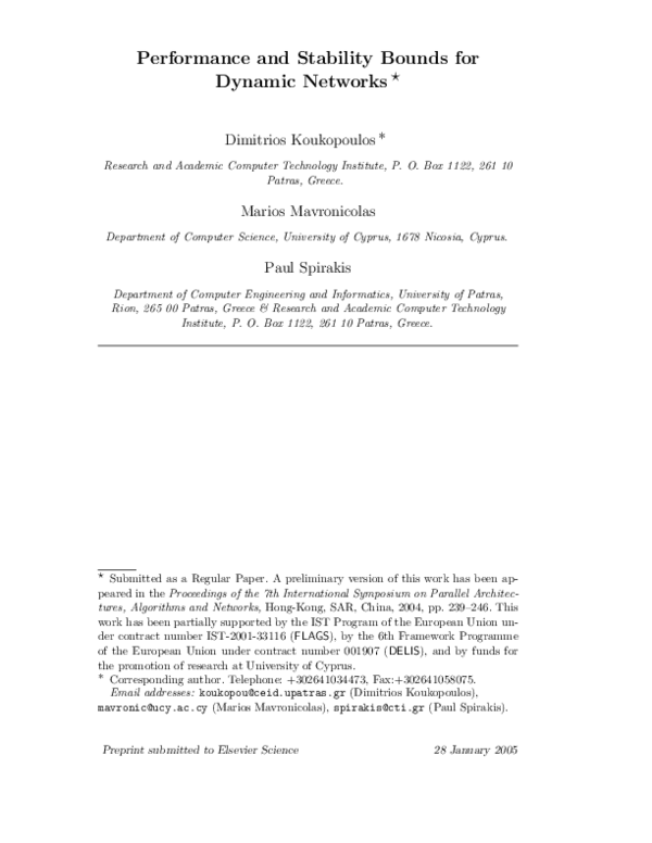3.2.1 The Construction of G For any integer k ≥ 2, consider the complete binary tree G0 (k) of height k, with all edges directed towards the root v0 . Furthermore, assign to every node v of G0 (k) a binary string s(v), called the label of node v, as follows: • s(v0 ) = ǫ (the empty string). • For each level l of G0 (k) (1 ≤ l ≤ k) order the nodes at level l from left to right and number them with the integers 1, . . . , 2l . For each such node v of order m (1 ≤ m ≤ 2l ), s(v) will be the binary representation of m − 1 that uses l bits. From the definition of the label function s, it immediately follows: Lemma 3.7 For each internal node v of G0 (k), s(v) is the longest common prefix of all s(u), where u runs over the two children of v. PROOF. Assume that v has order m, so that s(v) = b(m − 1), and consider any child u of v. Clearly, the order of u is either 2m − 1 or 2m. Hence, s(u) is the binary representation b of either 2m − 2 or 2m − 1. But, b(2m − 2) = b(2(m − 1)) = b(m − 1)0 and b(2m − 1) = b(2m − 2 + 1) = b(2m − 2) + b(1) = b(m−1)0+b(1) = b(m−1)0. Thus, s(v) is the longest common prefix (b(m−1)) of the two s(u), where u is a child of v, as needed. ✷ Modify now the network G0 (k) to obtain the network G(k), as follows: • For each internal node v: · Remove the edge (vl , v) pointing to v from its left child vl . 17 0 1 00 000 0000 01 001 010 0001 0100 10 011 100 0101 11 101 1001 110 111 1101 1111 Fig. 2. The network G(4) ′ · Add a node vl and the edges (vl , vl′ ) and (vl′ , v). Note that the resulting network G(k) is a subgraph of the complete binary tree of height 2k. Figures 1 and 2 illustrate the networks G0 (4) and G(4) providing the labels of many nodes. 3.2.2 Preliminaries For each node v in the network G0 (k), denote Z(v) the number of 0s in the string s(v). Note that the distance of node v from the root is different in the network G(k) than in the network G0 (k). In particular, the distance of node v from the root is |s(v)| for G0 (k), while it is |s(v)| + Z(v) for G(k). The additional term Z(v) accounts for the number of nodes added in the path from v to the root, which is, by construction, the number of 0s in Z(v) (since a node is added for each node in the path that is a left child). For each leaf v in G0 (k), define D(v) to be the predecessor node u of v in G0 (k) that is closest to v and v is a descendant of, or equal to, the left child of a child of D(v), or the root, if no such predecessor u exists. The definition of D(v) immediately implies: For each leaf v in G0 (k), D(v) is the node on the path from v to the root, such that s(D(v)) is obtained by removing the least significant bits from s(v) till either one bit after the first 0 has been removed, or the empty string has been obtained. 3.2.3 The Adversary Initial system configuration. We assume that, initially (t = 0), there is a number of packets that are queued at each leaf requiring to traverse only the 18 out-going edge of the leaf where they are queued. The number of leafs of G(k) is 2k . In the queue at the tail of the out-going edge of leaf v there is initially queued a number of wC + k − Z(v) packets. Adversary‘s behavior. The out-going edge of each leaf v has unit capacity at the time interval [0, k − Z(v)). Therefore, at each one of these time steps one packet from the initial ones leaves the system at each out-going edge. Till the time k − Z(v) + w all the packets that are queued initially in a leaf v have packets to been absorbed. At time step k − Z(v), the adversary injects wρC 2 each leaf node v targeted with node D(v). The path that is assigned to these paths has capacity C at the time interval [k − Z(v), k − Z(v) + w − 1], while after this time the path changes capacity to unit (only the edges that do not overlap with paths that are used for packet injections at other time steps). 3 Adversarial model restriction. In order to guarantee that this adversary is a valid one, we should show that the packets that want to traverse any common edge with capacity C at the time of their injection cannot be more than wρC packets, it suffices to packets. Because the adversary injects in any leaf wρC 2 show that any edge is used at most by the packet flows that are injected in two leaves. Note that if a packet that is injected to a leaf v wants to reach the nodes u1 and u2 of the original tree there are two cases depending on whether these nodes are neighbors or not. If these nodes are neighbors, the packet should traverse the edge (u1 , u2 ), otherwise it should traverse the edges ′ ′ (u1 , u1 ) and (u1 , u2 ). For this purpose, the k − |s(u1 )| − 1 least significant bits of s(v) must all be 1’s, and the |s(u1 )| most significant bits of |s(v)| must all match the corresponding bits of s(u1 ). This can happen for at most two leaves. Thus, at most two leaves send packets that traverse any edge, and therefore any edge is used by at most wρC packets. Evolution of the System Configuration. We show here the evolution of the system configuration at any internal node of the network Gk . Claim 3.8 Consider any node v of G0 (k) such that |s(v)| ≤ k − 2. Then, all packets that traverse v arrive at v between time (k − |s(v)| − 1) wCρ + 2k − 2 wCρ Z(v) − |s(v)| + w − 1 and time (k − |s(v)|) 2 + 2k − Z(v) − |s(v)| + w − 2. PROOF. We prove this by induction on k − |s(v)|, i.e., on the height of the node v. Basis case: Let v be any node such that |s(v)| = k − 2, let vr be the right child ′′ of v, and let vl be the left child of v in G0 (k). Note that s(vl ) = s(v)0. Let vl ′ be the right child of vl , and let vl be the left child of vl in G0 (k). 3 For simplicity, we assume here that to remove. wρC 2 19 is an integer, but this assumption is easy At time k−Z(vl ), the adversary injects wCρ packets in vl requiring to traverse a 2 ′ path with edges that have capacity C. After time k−Z(vl )+w−1, the capacity packets follow to reach vl changes to unit. Therefore, these of the edges the wCρ 2 ′ packets arrive, one per time step, to vl starting at time k − Z(vl ) + 1 + w. Since ′ ′ ′ s(vl ) = s(vl )0, then Z(vl ) = Z(vl ) + 1. Thus, k − Z(vl ) + 2 = k − Z(vl ) + 1. ′′ ′′ The packets that vl receives from vl are injected by the adversary to vl at ′′ ′ ′′ time k − Z(vl ) = k − Z(vl ). So, the packets from vl and vl arrive at vl at exactly the same time steps. ′ ′ ′ But, the packets coming to vl from vl have been in the system longer than ′′ the packets coming to vl from vl . So, they will have priority over the pack′ ′′ ets coming from vl . However, packets coming to vl from vl have v as final destination (they are absorbed at v). Thus, the first of the packets that v ′′ receives from vl which will be forwarded on (packets coming from vl ) arrives at v at time [k − Z(vl ) + 1] + wρC + 1 + w, and the remainder arrive 2 wCρ one per time step for the next 2 − 1 time steps because they follow a path with unit capacity. Since Z(vl ) = Z(v) + 1 and |s(v)| = k − 2, we take + 1 + w = (k − |s(v)| − 1) wρC + 2k − Z(v) − |s(v)| + w − 1. [k − Z(vl ) + 1] + wρC 2 2 This means that exactly one of those packets arrives at v at every time step + 2k − Z(v) − |s(v)| + w − 1, and time between time (k − |s(v)| − 1) wCρ 2 wCρ (k − |s(v)|) 2 + 2k − Z(v) − |s(v)| + w − 2. An analogous fact holds for the packets arriving at v from vr that are forwarded onward by v. Inductive hypothesis: For any node v of G0 (k), the packets that traverse v + 2k − Z(v) − |s(v)| + w − 1 and time arrive at v between time (j − 1) wCρ 2 wCρ j 2 + 2k − Z(v) − |s(v)| + w − 2 for k − |s(v)| = j. ′ ′ Induction step: We assume the claim for all v such that k −|s(v )| ≤ j. Choose any v such that k − |s(v)| = j + 1. Let vr be the right child of v, and let vl be the left child of v in G0 (k). By the inductive hypothesis, the packets that vl forwards to v arrive at vl between time (j − 1) wCρ + 2k − Z(vl ) − |s(vl )| + w − 1 2 wCρ and time j 2 + 2k − Z(vl ) − |s(vl )| + w − 2. Of these packets, the ones that ′ vl receives from its left child have been originated at a node vl such that ′ s(vl ) = s(vl )01j−1 , and the ones that vl receives from its right child have been ′′ ′ ′ ′′ originated at a node vl such that s(vl ) = s(vl )1j . Since Z(vl ) = Z(vl ) + 1, all the packets that vl receives from its left child have been in the system longer than the packets that vl receives from its right child. Thus, all the packets that vl receives from its left child have priority over any packet that vl receives from its right child. Since vl receives one packet to forward per time step from each of its children, all the packets, which have v as their destination, are forwarded before any packet that has to go further. packets that vl forwards to v having v as a final destination. There are wCρ 2 Thus, the packets that v receives from vl that need to be forwarded arriving 20 at v between time j wCρ + 2k − Z(vl ) − |s(vl )| + 1 + w, and time (j + 1) wCρ + 2 2 2k − Z(vl ) − |s(vl )| + w. Since |s(vl )| = |s(v)| + 1 and Z(vl ) = Z(v) + 1, these + 2k − Z(v) − |s(v)| + w − 1 time steps are between time (k − |s(v)| − 1) wCρ 2 wCρ and time (k − |s(v)|) 2 + 2k − Z(v) − |s(v)| + w − 2. Note that exactly one of those packets arrives at v at each time step. A similar argument shows that at each time step in which v receives a packet from vl to forward it onward, it also receives a packet from vr for forwarding. ✷ Proof of the Theorem 3.6. The theorem follows from the fact that the longest path that leads to any node v is i = 2(k − |s(v)|). By Claim 3.8, packets destined for v reach vr , the right child of v, no earlier than time (k − |s(vr )| − +2k−Z(vr )−|s(vr )|+w−1. The last of these packets will reach v at time 1) wCρ 2 +2k−Z(vr )−|s(vr )|+w−1. These packets are inserted at a leaf (k−|s(vr )|) wCρ 2 ′ ′ ′ v such that s(v ) = s(vr )01k−|s(vr )|−1 at time step k−Z(v ) = k−Z(vr )−1 and the path that is assigned to them has capacity C. Thus, the total time spent +k −|s(vr )|+w. Substituting in the system by these packets is (k −|s(vr )|) wCρ 2 wCρ |s(v)| + 1 for |s(vr )|, this is (k − |s(v)| − 1)( 2 + 1) + w = Ω(iwCρ). The largest queue required for the adversary construction is wC + k. For k = C, we take wC + C = (w + 1)C. 4 SIS on Directed Acyclic Graphs In this section, we present lower bounds on the performance of SIS on DAGs. Recall that we consider DAGs, in which nodes are ordered by the topological order induced by the graph. This order assigns to each node v a level i ≥ 0, denoted level(v), such that the longest path leading to node v has length i. We show: Theorem 4.1 There is a directed acyclic graph G and an adversary Aw,ρ such that in the system G,A,SIS any packet with destination a node v of G at level i suffers a delay of Ω(iwCρ) time steps, while the largest queue required is (w + 3)C. The proof of Theorem 4.1 is similar to the proof of Theorem 3.6. Again, for any integer k ≥ 2 we consider the complete binary tree of height k, G0 (k), where a binary string s(v), called the label of node v, is assigned to every node v as in Theorem 3.6 (Figure 1 illustrates the network G0 (4) providing the labels of many nodes.) We construct similarly to Theorem 3.6 the network G(k) that is a subgraph of the complete binary tree of height 2k (Figure 2 illustrates the network G(4).) The only difference to the proof of Theorem 3.6 is the construction of the adversary. 21 4.1 The Adversary Initial system configuration. We assume that, initially (t = 0), there is a number of packets that are queued at each leaf requiring to traverse only the out-going edge of the leaf where they are queued. The number of leafs of G(k) is 2k . In the queue at the tail of the out-going edge of leaf v with order m from left to right where m takes on odd values from the integer interval [1, 2k ], there are queued wC + k − (k − Z(v)) packets requiring to traverse only the queue where they have been injected. Also, we assume that, initially at each leaf v with order m from left to right, where m takes on even values from the integer interval [1, 2k ], there are queued (w + 2)C + k − (k − Z(v)) packets requiring to traverse only the queue where they have been injected. Adversary‘s behavior. The out-going edge of each leaf v has unit capacity at the time interval [0, Z(v)). Therefore, at each one of these time steps one packet from the initial ones leaves the system at each out-going edge. Till the time Z(v) + w + 2, all the packets that are queued initially in a leaf v have been absorbed. At time step Z(v), the adversary injects wρC packets to each leaf node v tar2 geted with node D(v). The path that is assigned to these packets has capacity C at the time interval [Z(v), Z(v) + w − 1] for any leaf v with order m that takes on odd values from the integer interval [1, 2k ]. Also, the path that is assigned to these packets has capacity C at the time interval [Z(v), Z(v)+w + 1] for any leaf v with order m that takes on even values from the integer interval [1, 2k ]. After this time the path changes capacity to unit (only the edges that do not overlap with paths that are used for packet injections at other time steps). Adversarial model restriction. Its similar to the corresponding part of the proof of Theorem 3.6. Evolution of the System Configuration. We show here the evolution of the system configuration at any internal node of the network Gk . Claim 4.2 Consider any node v of G0 (k) such that |s(v)| ≤ k − 2. Then, all packets that traverse v arrive at v between time (k −|s(v)|−1) wCρ +k +Z(v)− 2 wCρ |s(v)| + w + 3 + 2(k − |s(v)| − 1) − 2 and time (k − |s(v)|) 2 + k + Z(v) − |s(v)| + w + 2 + 2(k − |s(v)|) − 4. PROOF. We prove this by induction on k − |s(v)|, i.e., on the height of the node v. Basis case: Let v be any node such that |s(v)| = k − 2, let vr be the right child 22 ′′ of v, and let vl be the left child of v in G0 (k). Note that s(vl ) = s(v)0. Let vl ′ be the right child of vl , and let vl be the left child of vl in G0 (k). packets in vl requiring to traverse a At time Z(vl ), the adversary injects wCρ 2 ′ path with edges that have capacity C. After time Z(vl ) + w − 1, the capacity packets follow to reach vl changes to unit. Therefore, of the edges the wCρ 2 ′ these packets arrive, one per time step, to vl starting at time Z(vl ) + 1 + w. ′ ′ ′ Since s(vl ) = s(vl )0, then Z(vl ) = Z(vl ) + 1. Thus, Z(vl ) + 2 = Z(vl ) + 3. The ′′ ′′ packets that vl receives from vl are injected by the adversary to vl at time ′′ ′ ′′ Z(vl ) = Z(vl ). So, the packets from vl and vl arrive at vl at exactly the same time steps. ′ ′ ′ But, the packets coming to vl from vl have been in the system shorter than ′′ the packets coming to vl from vl . So, they will have priority over the packets ′ ′′ coming from vl . However, packets coming to vl from vl have v as final destination (they are absorbed at v). Thus, the first of the packets that v receives ′′ from vl which will be forwarded on (packets coming from vl ) arrives at v at time [Z(vl ) + 3] + wρC + 1 + w, and the remainder arrive one per time step 2 wCρ for the next 2 − 1 time steps because they follow a path with unit capacity. +1+w = Since Z(vl ) = Z(v) + 1 and |s(v)| = k − 2, we take [Z(vl ) + 3] + wρC 2 wρC (k − |s(v)| − 1) 2 + k + Z(v) − |s(v)| + w + 3 + 2(k − |s(v)| − 1) − 2. This means that exactly one of those packets arrives at v at every time step between time + k + Z(v) − |s(v)| + w + 3 + 2(k − |s(v)| − 1) − 2, and time (k − |s(v)| − 1) wCρ 2 wCρ (k − |s(v)|) 2 + k + Z(v) − |s(v)| + w + 2 + 2(k − |s(v)|) − 4. An analogous fact holds for the packets arriving at v from vr that are forwarded onward by v. Inductive hypothesis: For any node v of G0 (k), the packets that traverse v + k + Z(v) − |s(v)| + w + 3 + 2(j − 1) − 2 arrive at v between time (j − 1) wCρ 2 wCρ and time j 2 + k + Z(v) − |s(v)| + w + 2 + 2j − 4 for k − |s(v)| = j. ′ ′ Induction step: We assume the claim for all v such that k −|s(v )| ≤ j. Choose any v such that k − |s(v)| = j + 1. Let vr be the right child of v, and let vl be the left child of v in G0 (k). By the inductive hypothesis, the packets that vl + k + Z(vl ) − |s(vl )| + w + forwards to v arrive at vl between time (j − 1) wCρ 2 3 + 2(j − 1) − 2 and time j wCρ + k + Z(vl ) − |s(vl )| + w + 2 + 2j − 4. Of these 2 packets, the ones that vl receives from its left child have been originated at ′ ′ a node vl such that s(vl ) = s(vl )01j−1 , and the ones that vl receives from its ′ ′′ right child have been originated at a node vl such that s(vl ) = s(vl )1j . Since ′′ ′ Z(vl ) = Z(vl ) + 1, all the packets that vl receives from its left child have been in the system shorter than the packets that vl receives from its right child. Thus, all the packets that vl receives from its left child have priority over any packet that vl receives from its right child. Since vl receives one packet to forward per time step from each of its children, all the packets, which have v 23 as their destination, are forwarded before any packet that has to go further. packets that vl forwards to v having v as a final destination. There are wCρ 2 So, the packets that v receives from vl that need to be forwarded arriving + k + Z(vl ) − |s(vl )| + 3 + w + 2j − 2, and at v between time step j wCρ 2 wCρ time step (j + 1) 2 + k + Z(vl ) − |s(vl )| + w + 2 + 2(j + 1) − 4. Since |s(vl )| = |s(v)| + 1 and Z(vl ) = Z(v) + 1, these time steps are between time + k + Z(v) − |s(v)| + w + 3 + 2(k − |s(v)| − 1) − 2 step (k − |s(v)| − 1) wCρ 2 + k + Z(v) − |s(v)| + w + 2 + 2(k − |s(v)|) − 4. and time step (k − |s(v)|) wCρ 2 Note that exactly one of those packets arrives at v at each time step. A similar argument shows that at each time step v receives a packet from vl to forward it onward, it also receives a packet from vr for forwarding. ✷ Proof of the Theorem 4.1. The theorem follows from the fact that the longest path that leads to any node v is i = 2(k − |s(v)|). By Claim 4.2, packets destined for v reach vr , the right child of v, no earlier than time (k − |s(vr )| − +k+Z(vr )−|s(vr )|+w+3+2(k−|s(vr )|−1)−2. The last of these packets 1) wCρ 2 +k+Z(vr )−|s(vr )|+w+3+2(k−|s(vr )|)−4. will reach v at time (k−|s(vr )|) wCρ 2 ′ ′ These packets are inserted at a leaf v such that s(v ) = s(vr )01k−|s(vr )|−1 ′ at time step Z(v ) = Z(vr ) + 1 and the path that is assigned to them has capacity C. Thus, the total time spent in the system by these packets is + k − |s(vr )| + w + 3 + 2(k − |s(vr )|) − 4. Substituting |s(v)| + 1 (k − |s(vr )|) wCρ 2 + k − |s(v)| − 1 + w + 3 + 2(k − |s(v)| − for |s(vr )|, this is (k − |s(v)| − 1) wCρ 2 wCρ 1) − 4 = (k − |s(v)| − 1)( 2 + 3) + w − 1 = Ω(iwCρ). The largest queue required for the adversary construction is (w + 2)C + k. For k = C, we take (w + 2)C + C = (w + 3)C. 5 Sufficient Conditions for Stability In this section, we present upper bounds on stability thresholds. We denote d(G) the length of the longest directed path that may be followed by any packet. We still consider the model of dynamic capacities [6] where each link capacity may take on integer values from [1, C]. We first show: 1 . For any network G, any adversary Aw,ρ and Theorem 5.1 Let ρ ≤ C(d(G)+1) any greedy protocol P, the system G, A, P is stable. PROOF. It suffices to show that any packet that arrives at a queue at time t, leaves this queue by time t + ⌊wρ⌋. Our proof is by induction on time t. Basis case: Consider any t ≤ d(G)wρ + 1. Let p be a packet that arrives to the queue e at time t ≤ d(G)wρ + 1. The edge e has unit capacity in the time 24 interval [t, t+⌊wρ⌋] in the worst-case (unit capacity permits the preservation of the biggest number of packets in the queue). Assume towards a contradiction that p is at the same queue at the end of time t + ⌊wρ⌋. This means that for each of the ⌊wρ⌋ time steps in [t + 1, t + ⌊wρ⌋] some other packet was sent over edge e due to the use of a greedy protocol. From the definition of the adversary, the largest number of packets that can be injected into the system by the end of time t + ⌊wρ⌋ − 1 requiring edge e is ⌊wρC⌋ + 1 packets because C is the capacity value of edge e at injection time that maximizes the number of packets that can be injected into the system requiring e (these are the packet p itself, and the ⌊wρC⌋ packets that were sent over e). Since t ≤ d(G)wρ + 1, we have t + ⌊wρ⌋ − 1 ≤ (d(G) + 1)wρ. By the definition of the adversary, the number of packets that require e and ′ they are injected by the end of any time step t ≤ (d(G) + 1)wρ is at most ⌈(d(G) + 1)ρ⌉⌊wρC⌋ because C is the capacity value of edge e at injection time that maximizes the number of packets that can be injected into the 1 , this is at most ⌊wρ⌋. A system requiring e. Since we assume ρ ≤ C(d(G)+1) contradiction to the fact that we identified ⌊wρ⌋ + 1 packets. ′ Inductive hypothesis: Any packet that arrives at some queue at time t ≤ t, ′ leaves the queue by time step t + ⌊wρ⌋. Induction step: We now prove the claim for any t > d(G)wρ + 1. Let p be a packet that arrives to the queue e at some time t. Consider any packet that requires edge e and it is injected by time t − d(G)⌊wρ⌋. By the inductive hypothesis, we know that such a packet left the queue where it was injected by time t − d(G)⌊wρ⌋ + ⌊wρ⌋, left the next queue by time t − d(G)⌊wρ⌋ + 2⌊wρ⌋, etc. I.e., it arrived to its destination by time t−d(G)⌊wρ⌋+d(G)⌊wρ⌋ = t (since the length of its path is at most d(G), and all its “arrival times” are earlier than t, so the inductive hypothesis holds). It follows that any packet that can delay packet p from going over edge e must be injected at time t − wρd(G) + 1 or later. Now assume towards a contradiction that packet p is still at queue e at the end of time t + ⌊wρ⌋. So, there are some other packets that crossed edge e in [t + 1, t + ⌊wρ⌋]. These packets are present in the network at the end of time t or later, and they are injected by time t + ⌊wρ⌋ − 1. However, we know that any packet that has been injected by time t − d(G)⌊wρ⌋, it has already left the network by the end of time t. Thus those packets must have been injected in the time interval [t − d(G)⌊wρ⌋ + 1, t + ⌊wρ⌋ − 1]. There are ⌊wρ⌋(d(G) + 1) − 1 time steps in this interval. So, the number of packets that require e that can be injected during this interval is bounded by ⌈(d(G) + 1)ρ⌉⌊wρC⌋ because C is the capacity value of edge e at injection time that maximizes the number of 1 packets that can be injected into the system requiring e. Since ρ ≤ C(d(G)+1) this is at most ⌊wρ⌋, a contradiction. ✷ 25 Now, we will show how we can relax the obtained stability condition for time priority protocols, such as FIFO and LIS. A time priority protocol is any greedy protocol that forwards a packet arriving at a queue at time t against any other packet that is injected into the system after time t. We show: 1 . For any network G, any adversary Aw,ρ and Theorem 5.2 Let ρ ≤ Cd(G) any time-priority protocol P, the system G, A, P is stable. PROOF. It suffices to show that any packet that arrives at a queue at time t, leaves this queue by time t + ⌊wρ⌋. Our proof is by induction on time t. Basis case: Consider any t ≤ d(G)wρ. Let p be a packet that arrives at queue e at time t ≤ d(G)wρ. Assume towards a contradiction that p is at the same queue at the end of time t + ⌊wρ⌋. Since the protocol is greedy and the edge e has unit capacity in the time interval [t, t + ⌊wρ⌋] in the worst-case (unit capacity permits the preservation of the biggest number of packets in the queue), there are at least ⌊wρ⌋ + 1 packets that traverse edge e in the time interval [t, t + ⌊wρ⌋] (these are p, and the packets that were sent over e in the interval [t, t + ⌊wρ⌋]). However, since the protocol is time priority, these packets must have been injected into the system by the end of time step t (otherwise they cannot delay p). By the definition of the adversary, the number of packets that may use e and they are injected into the system by the end of time t is at most ⌈t/w⌉⌊wρC⌋ ≤ ⌈d(G)ρ⌉⌊wρC⌋ ≤ ⌊wρ⌋, since ρ ≤ 1/Cd(G), and C is the capacity value of the edge e at injection time that maximizes the number of packets that can be injected into the system requiring e. A contradiction to the fact that we identified ⌊wρ⌋ + 1 packets. ′ Inductive hypothesis: Any packet that arrives at some queue at time t ≤ t, ′ leaves the queue by time step t + ⌊wρ⌋. Induction step: We now prove the claim for any t > d(G)wρ. Assume by ′ induction that any packet that arrives at some queue at time t ≤ t, leaves ′ this queue by time t + ⌊wρ⌋. Let p be a packet that arrives at the queue of the edge e at time t. Assume towards a contradiction that packet p is still at e at the end of time t + ⌊wρ⌋. The edge e has unit capacity in the time interval [t, t + ⌊wρ⌋] in the worst-case. Then, there is a set of ⌊wρ⌋ + 1 distinct packets that use edge e in the time interval [t, t + ⌊wρ⌋]. Since we have a time priority protocol, all these packets were injected by the end of time t. Moreover, we now prove that all these packets were injected at time t − wρd(G) + 1 or later. Consider any packet q that was injected into the system by time t − d(G)⌊wρ⌋. By the inductive hypothesis, q left the first queue on its path by time t − d(G)⌊wρ⌋ + ⌊wρ⌋, left the next queue by time t − 26 d(G)⌊wρ⌋ + 2⌊wρ⌋, and so on. Hence, q arrived at its destination by time t − d(G)⌊wρ⌋ + d(G)⌊wρ⌋ = t: since the length of its path is at most d(G), all its “arrival times” are earlier than t, so we may apply the inductive hypothesis. Therefore, all the ⌊wρ⌋ + 1 packets that use e in the time interval [t, t + ⌊wρ⌋] must have been injected into the system in the time interval [t − d(G)⌊wρ⌋ + 1, t]. There are ⌊wρ⌋d(G) time steps in this interval, and therefore the number of packets that require e and they can be injected during this interval is bounded by ⌈d(G)ρ⌉⌊wρC⌋ since C is the capacity value of the edge e at injection time that maximizes the number of packets that can be injected into the system requiring e. Since ρ ≤ 1/Cd(G), the number of packets that are injected during the time interval [t − d(G)⌊wρ⌋ + 1, t] is at most ⌊wρ⌋. A contradiction to the fact that we identified ⌊wρ⌋ + 1 packets. ✷ 6 Discussion and Directions for Further Research In this work, we studied the impact of dynamically changing link capacities (link capacities can take on integer values from [1, C] with C > 1) on the performance bounds of the LIS and the SIS protocols on DAGs and we obtained stability bounds for greedy protocols running on arbitrary networks. We proved that the LIS and SIS protocols have linear performance bounds on DAGs and that there are polynomial stability thresholds for greedy protocols on arbitrary networks depending on the maximum link capacity C and the length of the longest network path. A careful inspection of the proofs of the lower bound for LIS obtained in this work reveals that they also hold in the more restrictive model, where link capacities stay fixed for time at least a constant of the number of packets in the system at the time when the capacity was last set. This model is called QuasiStatic Link Capacities Model [11]. Therefore, the tight bound we prove here for LIS implies some kind of collapse of a powerful model (Model of Dynamic Capacities) to a weaker one (QuasiStatic Link Capacities Model) that is, rather surprising. An interesting avenue for further research would be to determine performance bounds for other stable protocols on DAGs such as FTG and NTS in the model of dynamic capacities. Also, an interesting question is if LIS and SIS have polynomial performance bounds on general networks. 27 References [1] M. Adler, A. Rosén, Tight Bounds for the Performance of Longest-in-System on DAGs, in: Proceedings of the 19th Annual Symposium on Theoretical Aspects of Computer Science, Lecture Notes in Computer Science, Antibes–Juan Les Pins, France, Springer-Verlag, 2002, Vol. 2285, pp. 88–99. [2] M. Andrews, B. Awerbuch, A. Fernandez, J. Kleinberg, T. Leighton, Z. Liu, Universal Stability Results for Greedy Contention-Resolution Protocols, Journal of the ACM, 48 (1) (2001) 39–69. [3] M. Andrews, L. Zhang, The Effect of Temporary Sessions on Network Performance, in: Proceedings of the 11th Annual Symposium on Discrete Algorithms, San Francisco, California, USA, 2000, pp. 448–457. [4] R. Bhattacharjee, A. Goel, Instability of FIFO at Arbitrarily Low Rates in the Adversarial Queueing Model, in: Proceedings of the 44th Annual IEEE Symposium on Foundations of Computer Science, Cambridge, MA, USA, 2003, pp. 160–167. [5] A. Borodin, J. Kleinberg, P. Raghavan, M. Sudan, D. Williamson, Adversarial Queueing Theory, Journal of the ACM, 48 (1) (2001) 13–38. [6] A. Borodin, R. Ostrovsky, Y. Rabani, Stability Preserving Transformations: Packet Routing Networks with Edge Capacities and Speeds, in: Proceedings of the 12th Annual ACM-SIAM Symposium on Discrete Algorithms, Washington, DC, USA, 2001, pp. 601–610. [7] H. Chen, D. D. Yao, Fundamentals of Queueing Networks, Springer-Verlag, 2000. [8] J. Diaz, D. Koukopoulos, S. Nikoletseas, M. Serna, P. Spirakis, D. Thilikos, Stability and Non-Stability of the FIFO Protocol, in: Proceedings of the 13th Annual ACM Symposium on Parallel Algorithms and Architectures, Crete, Greece, 2001, pp. 48–52. [9] D. Koukopoulos, M. Mavronicolas, S. Nikoletseas, P. Spirakis, On the Stability of Compositions of Universally Stable, Greedy, Contention-Resolution Protocols, in: Proceedings of the 16th International Symposium on DIStributed Computing, Lecture Notes in Computer Science, Toulouse, France, Springer-Verlag, 2002, Vol. 2508, pp. 88–102. [10] D. Koukopoulos, M. Mavronicolas, S. Nikoletseas, P. Spirakis, The Impact of Network Structure on the Stability of Greedy Protocols, in: Proceedings of the 5th Italian Conference on Algorithms and Complexity, Lecture Notes in Computer Science, Rome, Italy, Springer-Verlag, 2003, Vol. 2653, pp. 251–263. Also, accepted in the Journal Theory of Computing Systems. [11] D. Koukopoulos, M. Mavronicolas, P. Spirakis, Instability of Networks with Quasi-Static Link Capacities, in: Proceedings of the 10th International Colloquium on Structural Information and Communication Complexity, Carleton Scientific, Umea, Sweden, 2003, pp. 179–194. 28 [12] D. Koukopoulos, S. Nikoletseas, P. Spirakis, Stability Issues in Heterogeneous and FIFO Networks under the Adversarial Queueing Model, in: Proceedings of the 8th International Conference on High Performance Computing, Lecture Notes in Computer Science, Hyderabad, India, Springer-Verlag, 2001, Vol. 2228, pp. 3–14. Invited Keynote Address. [13] Z. Lotker, B. Patt-Shamir, A. Rosén, New Stability Results for Adversarial Queueing, in: Proceedings of the 15th Annual ACM Symposium on Parallel Algorithms and Architectures, Winnipeg, Manitoba, Canada, 2002, pp. 192–199. [14] C. Scheideler, B. Vöcking, From Static to Dynamic Routing: Efficient Transformations of Store-and-Forward Protocols, in: Proceedings of the 31st ACM Symposium on the Theory of Computing, 1999, Atlanta, Georgia, USA, pp. 215–224. 29