A Multitask Multiple Kernel Learning Algorithm for Survival Analysis
with Application to Cancer Biology
Onur Dereli 1 Ceyda Oğuz 2 Mehmet Gönen 2 3 4
Abstract
Predictive performance of machine learning algorithms on related problems can be improved
using multitask learning approaches. Rather than
performing survival analysis on each data set to
predict survival times of cancer patients, we developed a novel multitask approach based on multiple kernel learning (MKL). Our multitask MKL
algorithm both works on multiple cancer data sets
and integrates cancer-related pathways/gene sets
into survival analysis. We tested our algorithm,
which is named as Path2MSurv, on the Cancer
Genome Atlas data sets analyzing gene expression profiles of 7,655 patients from 20 cancer
types together with cancer-specific pathway/gene
set collections. Path2MSurv obtained better or
comparable predictive performance when benchmarked against random survival forest, survival
support vector machine, and single-task variant of
our algorithm. Path2MSurv has the ability to identify key pathways/gene sets in predicting survival
times of patients from different cancer types.
1. Introduction
Understanding the formation and progression mechanisms
of the diseases plays a vital importance in treating them.
To this aim, genomic characterizations have been used in
answering various research problems. Survival analysis
is one of these research problems that aims to predict survival times of patients. There are several machine learning
algorithms developed to predict survival times using genomic characterizations and clinical information of patients
(Cox, 1972; Cox & Oakes, 1984; Bakker et al., 2004; Shivaswamy et al., 2007; Evers & Messow, 2008; Ishwaran et al.,
2008; Khan & Zubek, 2008; Van Belle et al., 2011a;b; Mogensen & Gerds, 2013; Kiaee et al., 2016; Wang et al., 2016;
Yousefi et al., 2017). These existing algorithms consider
the censored observations, but most of them cannot handle high-dimensional feature representations (e.g., genomic
characterizations) effectively due to the limited number of
training samples. These standard algorithms were recently
shown to be more suitable for low-dimensional feature representations (i.e., clinical variables) (Yuan et al., 2014).
Pathways/gene sets are simply the sets of genes with roles
in the same or similar biological mechanisms. Relating
pathways/gene sets to clinical phenotypes helps us better
understand the underlying mechanisms of diseases. That is
why several machine learning algorithms were proposed to
identify pathways/gene sets associated with disease-related
phenotypes such as overall survival time after diagnosis.
These algorithms either (i) identify survival-related molecular mechanisms using feature selection and learn a survival
analysis model on selected features only or (ii) train a survival analysis model on each pathway/gene set separately
and pick survival-related ones by comparing their predictive
performances (Pang et al., 2012; Zhang et al., 2017; Pang
et al., 2010; 2011). However, both approaches have drawbacks. The first approach might pick biologically unrelated
genes due to highly correlated structure of genomic characterizations. The second approach might pick related or
similar pathways/gene sets due to the fact that each pathway/gene set is analyzed separately. To eliminate these
problems, pathway/gene set collections should be integrated
into the model during the training step, so that learning algorithm can pick informative pathways/gene sets in a more
robust manner.
1
Graduate School of Sciences and Engineering, Koç University,
İstanbul 34450, Turkey 2 Department of Industrial Engineering,
College of Engineering, Koç University, İstanbul 34450, Turkey
3
School of Medicine, Koç University, İstanbul 34450, Turkey
4
Department of Biomedical Engineering, School of Medicine, Oregon Health & Science University, Portland, OR 97239, USA. Correspondence to: Mehmet Gönen <mehmetgonen@ku.edu.tr>.
Proceedings of the 36 th International Conference on Machine
Learning, Long Beach, California, PMLR 97, 2019. Copyright
2019 by the author(s).
Using high-dimensional genomic characterizations in machine learning algorithms is a challenging task due to their
highly correlated structures. Kernel-based machine learning
algorithms were used to address this problem in survival
analysis (Shivaswamy et al., 2007; Evers & Messow, 2008;
Khan & Zubek, 2008; Van Belle et al., 2011a;b). Kernel
methods were also shown to be very successful in other
cancer-related problems such as drug sensitivity predic-
�A Multitask Multiple Kernel Learning Algorithm for Survival Analysis
tion (Costello et al., 2014) and gene essentiality prediction
(Gönen et al., 2017). The success of kernel methods lies
mainly in the fact that the number of model parameters optimized is proportional to the number of samples not to the
number of features (Schölkopf & Smola, 2002).
The kernel function that defines a similarity measure between pairs of samples is the most important component of
kernel methods. No single kernel function is the best one
for different problems. That is why we can use a weighted
combination of several kernel functions instead of using
a single kernel, which is known as multiple kernel learning (MKL) (Gönen & Alpaydın, 2011). Following this
idea, an MKL-based survival analysis algorithm can pick
informative pathways/gene sets by assigning zero weight to
uninformative ones during inference. This approach defines
a kernel function on each pathway/gene set using genomic
features of the genes included. MKL part then learns an
optimized kernel function, which is used to predict survival
times (Dereli et al., in press).
Multitask learning aims to mainly model related problems
conjointly by exploiting commonalities between them (Caruana, 1997). This idea has also been applied in cancer studies
to improve predictive performance (Costello et al., 2014;
Gönen et al., 2017). Recently, studies modeling multiple
cancer types simultaneously (i.e., pan-cancer studies) to
capture common underlying biological mechanisms have attracted great attention (The Cancer Genome Atlas Research
Network et al., 2013; Yang et al., 2014; Anaya et al., 2016).
However, to the best of our knowledge, there is a limited
number of multitask learning methods for survival analysis
(Li et al., 2016; Wang et al., 2017).
In this study, we combined survival analysis, MKL (for pathway selection) and multitask learning (for modeling multiple
cohorts) in a unified formulation for the first time. Our algorithm can identify survival-related biological pathways/gene
sets using high dimensional genomic characterizations of
patients from multiple cohorts.
2. Related Work
Random forest (RF) is a supervised machine learning algorithm originally developed for regression and classification
(Breiman, 2001). It first creates multiple decision trees using randomly selected features from the input features or
randomly selected samples from the training data. It then
combines these decision trees to obtain more robust predictions. RF was also extended towards survival analysis and
successfully used in many studies (Ishwaran et al., 2008).
Support vector machine (SVM) is another supervised machine learning algorithm originally developed for binary
classification (Cortes & Vapnik, 1995). SVM was also extended towards censored regression problems, i.e., survival
analysis (Shivaswamy et al., 2007; Khan & Zubek, 2008).
Survival SVM can be formulated as follows:
N
X
1
(ξi+ + (1 − δi )ξi− )
min. w⊤ w + C
2
i=1
w.r.t. w ∈ RD , ξ + ∈ RN , ξ − ∈ RN , b ∈ R
s.t. ǫ + ξi+ ≥ yi − w⊤ xi − b
ǫ+
ξi−
ξi+
ξi−
≥0
∀i
≥0
∀i,
⊤
≥ w xi + b − y i
(1)
∀i
∀i
N
where the training data set is {(xi , δi , yi )}i=1 , N is the
number of samples, xi is the feature vector of sample i, δi ∈
{0, 1} is the binary indicator variable that shows whether the
observed survival time of sample i is censored (i.e., δi = 1)
or not (i.e., δi = 0), and yi ∈ R is the observed survival
time of sample i (i.e., time to last follow-up if censored or
time to death if uncensored). Here, w is the set of weights
assigned to features, C is the non-negative regularization
parameter, ξ + and ξ − are the sets of slack variables, D
is the number of input features, ǫ is the non-negative tube
width parameter, and b is the bias parameter.
The primal optimization problem in (1) has (D + 2N + 1)
decision variables, which makes the model computationally
very costly. To integrate kernel functions into this formulation via standard kernel trick, the corresponding Lagrangian
function is written as
N
X
1
L = w⊤ w + C
(ξi+ + (1 − δi )ξi− )
2
i=1
−
N
X
αi+ (ǫ + ξi+ − yi + w⊤ xi + b)
i=1
−
N
X
αi− (ǫ + ξi− − w⊤ xi − b + yi )
i=1
−
N
X
βi+ ξi+ −
N
X
βi− ξi− .
i=1
i=1
The derivatives of the Lagrangian function with respect to
the decision variables of the primal problem are found as
N
X
∂L
= 0⇒w=
(αi+ − αi− )xi
w
i=1
N
X
∂L
(αi+ − αi− ) = 0
= 0⇒
∂b
i=1
∂L
= 0 ⇒ C = αi+ + βi+
∀i
∂ξi+
∂L
= 0 ⇒ C(1 − δi ) = αi− + βi−
∂ξi−
∀i.
�A Multitask Multiple Kernel Learning Algorithm for Survival Analysis
Using the Lagrangian function and these derivatives, the
corresponding dual optimization problem is written as
min. −
N
X
yi (αi+
−
αi− )
+ǫ
+
2
(αi+
−
αi− )(αj+
s.t.
−
Nt
Nt
w.r.t. wt ∈ RDt , ξ +
t ∈ R , ξ t ∈ R , bt ∈ R
+
s.t. ǫ + ξti
≥ yti − w⊤
t xti − bt
−
αj− )x⊤
i xj
i=1 j=1
w.r.t. α+ ∈ RN , α− ∈ RN
N
X
(αi+ + αi− )
i=1
i=1
N N
1 XX
N
X
optimization problem of our formulation can be written as
#
"
Nt
T
X
X
1 ⊤
+
−
(ξti
+ (1 − δti )ξti
)
min.
wt wt + C
2
t=1
i=1
(2)
(αi+ − αi− ) = 0
i
C ≥ αi+ ≥ 0
C(1 − δi ) ≥
∀i
αi−
≥0
∀i.
The dual optimization problem in (2) has 2N decision variables instead of (D + 2N + 1), which significantly reduces
the computational complexity. By replacing the term x⊤
i xj
with a kernel function k(xi , xj ), kernel functions can be
integrated into the model.
Several recent studies showed that different cancer types
have similar or same underlying biological mechanisms
(The Cancer Genome Atlas Research Network et al., 2013;
Choi et al., 2014; Damrauer et al., 2014; Hoadley et al.,
2014; Lawrence et al., 2014; Yang et al., 2014; Khirade
et al., 2015; Pappa et al., 2015; Wan et al., 2015; Anaya
et al., 2016), which supports the joint modeling of multiple
diseases. That is why there are existing multitask machine
learning models to model multiple patient cohorts conjointly
(Li et al., 2016; Wang et al., 2017). However, these methods
use genomic features directly, and they are not able to extract
relative importance of pathways/gene sets.
The training data sets defined over multiple cohorts are given
Nt T
as {{(xti , δti , yti )}i=1
}t=1 , where T denotes the number
of tasks (i.e., cohorts), Nt represents the total number of
samples for task t, xti is the feature vector of sample i of
task t, δti is the binary indicator variable that shows whether
the observed survival time of sample i of task t is censored
(i.e., δti = 1) or not (i.e., δti = 0), and yti ∈ R is the
observed survival time of sample i of task t. The primal
+
ξti
−
ξti
≥0
∀(t, i)
≥0
∀(t, i),
≥
w⊤
t xti
∀(t, i)
+ bt − yti
(3)
∀(t, i)
where wt is the vector of weights assigned to features for
task t, C is the non-negative regularization parameter, ξ +
t
and ξ −
t are the sets of slack variables for task t, Dt is the
number of input features for task t, ǫ is the non-negative
tube width parameter, and bt is the bias parameter for task t.
We formulated the corresponding dual optimization problem, where we have a combined objective function over all
tasks with a single set of constraints on the kernel weights.
min.
T
X
Jt (η)
t=1
w.r.t. η ∈ RP
s.t.
P
X
(4)
ηm = 1
m=1
ηm ≥ 0
∀m.
The inner optimization model Jt (η) for each task is basically a single-kernel survival SVM defined as
min. −
Nt
X
+
−
yti (αti
− αti
)+ǫ
+
w.r.t.
s.t.
1
2
α+
t
Nt
X
Nt
Nt X
X
Nt
X
+
−
(αti
+ αti
)
i=1
i=1
3. Our Proposed Multitask MKL Algorithm
for Survival Analysis
We extended survival SVM algorithm towards multitask
learning and MKL, which is named as Path2MSurv (Figure 1a). By doing so, we will be able to model multiple
cohorts simultaneously and to extract survival-related pathways/gene sets to identify shared biological mechanisms
among these cohorts.
ǫ+
−
ξti
+
−
+
−
(αti
− αti
)(αtj
− αtj
)kη (xti , xtj )
i=1 j=1
Nt
∈ RN t , α −
t ∈R
(5)
+
−
(αti
− αti
)=0
i=1
+
C ≥ αti
≥0
C(1 − δti ) ≥
∀i
−
αti
≥0
∀i,
PP
where kη (xti , xtj ) corresponds to m=1 ηm km (xti , xtj ).
We are guaranteed to obtain a sparse set of kernel weights
P
in
PPPath2MSurv since η lies on a simplex, i.e., η ∈ R ,
m=1 ηm = 1, and ηm ≥ 0.
It is not possible to find the global optimal solution of
the overall optimization problem in (4) since it is not
jointly convex with respect to decision variables η and
�A Multitask Multiple Kernel Learning Algorithm for Survival Analysis
a
Multitask
multiple kernel learning
Patients
Genes
···
KT,1
···
XT,1
···
Genes
Days to
death
Days to last
follow-up
NA
364
..
.
678
NA
..
.
NA
520
2555
NA
Y1
XT,P
KT,P
η1
KT,η
Survival
analysis
ηP
···
···
Patients
···
···
Genes
Patients
Gene setP
Patients
G25
XT
Alive
Dead
···
···
···
G12
G47
Alive
Dead
..
.
f1
K1,η
Patients
G8
ηP
Vital
status
Patients
Patients
G19
···
K1,P
Genes
G42
η1
···
···
Patients
G19
Survival
analysis
Patients
Patients
G6
G3
X1,P
Patients
G28
X1
G42
K1,1
···
G17
X1,1
Patients
G1
Patients
Gene set1
Patients
Genes
Vital
status
Dead
Dead
..
.
fT
Alive
Dead
Patients
YT
Days to
death
Days to last
follow-up
456
3200
..
.
NA
NA
..
.
NA
1891
2208
NA
Patients
Patients
Patients
Genes
b
BLCA
● (402)
BRCA
(1067)
CESC COAD ESCA GBM HNSC
(291) (433) (160) (152) (498)
KIRC
(526)
KIRP LAML LGG
(285) (130) (506)
LUAD
(500)
LIHC
(365)
LUSC
(493)
OV PAAD READ SARC STAD
(372) (176) (156) (256) (348)
UCEC
(539)
Figure 1. Overview of the proposed Path2MSurv algorithm together with the summary of data sets used in our computational experiments.
(a) Path2MSurv algorithm takes gene expression profiles of patients from each cohort, i.e., {Xt }Tt=1 , a pathway/gene set collection with
P pathways/gene sets, and clinical information including vital status, days to death, and days to last follow-up, i.e., {Yt }Tt=1 , as its inputs.
T,P
It then calculates kernel matrices, i.e., {Kt,p }P
p=1 , on data matrix slices, i.e., {Xt,p }t=1,p=1 , obtained by mapping pathways/gene sets on
T
gene expression profiles. The weighted sums of these kernel matrices, i.e., {Kt,η }t=1 , are used to predict survival times of cancer patients
using the prediction functions, i.e., {f }Tt=1 . (b) Data sets used in our computational experiments and their corresponding numbers of
patients after filtering steps.
− T
{(α+
t , αt )}t=1 . Instead, we formulated an alternating optimization approach to the overall optimization problem by
following the idea proposed by Xu et al. (2010). Kernel
(s)
weights are initialized to uniform values, i.e., ηm = 1/P ,
at the first iteration, i.e., s = 0. In each iteration, using kernel weights η (s) , we solve the inner optimization problem in
(5) for each task to obtain its corresponding support vector
+(s)
−(s)
coefficients {αt , αt }. Kernel weights are then updated for the next iteration (s + 1) using the support vector
coefficients of all tasks in the following update equation:
s
Nt P
Nt
T
P
P
(s)
(s) (s)
ηm
αti αtj km (xti , xtj )
(s+1)
ηm
=
t=1
T P
P
P
i=1 j=1
(s)
ηo
t=1 o=1
(s)
s
Nt P
Nt
P
i=1 j=1
+(s)
−(s)
∀m,
(s) (s)
αti αtj ko (xti , xtj )
where αti = (αti − αti ). The convergence of this
alternating optimization approach is guaranteed since we
monotonically decrease the objective function value of (4).
�A Multitask Multiple Kernel Learning Algorithm for Survival Analysis
4. Experiments
4.1.2. PATHWAY /G ENE S ET DATABASES
We performed an extensive set of computational experiments on several cancer data sets, where we compared the predictive performance of our proposed method
Path2MSurv against survival RF (Ishwaran et al., 2008), survival SVM (Shivaswamy et al., 2007; Khan & Zubek, 2008),
and single-task variant of our algorithm (i.e., Path2Surv)
trained on each data set separately (Dereli et al., in press).
We used two pathway/gene set databases in addition to
gene expression profiles of primary tumors to understand
which biological mechanisms are predictive of overall survival times of cancer patients. We extracted gene sets in
Hallmark collection (Liberzon et al., 2015) and pathways in Pathway Interaction Database (PID)
collection (Schaefer et al., 2009) from the Molecular
Signatures Database (MSigDB) (http://software.
broadinstitute.org/gsea). These collections consist of group of genes that play joint roles in metabolism,
gene regulation, and signaling in cells. Hallmark is a
computationally constructed gene set collection including
50 gene sets with sizes between 32–200. It summarizes
and represents specific well-defined biological states or processes displaying coherent expression of gene sets. PID is
a manually curated and peer-reviewed pathway collection
including 196 human signaling and regulatory pathways
with sizes between 10–137.
4.1. Data Sets
We used gene expression profiles and clinical annotation
data of cancer patients provided by The Cancer Genome
Atlas (TCGA) at the Genomics Data Commons (GDC) data
portal (https://portal.gdc.cancer.gov). To integrate prior biological knowledge about cancer-specific
pathways/gene sets into our model, we used one pathway
and one gene set collection.
4.1.1. TCGA DATA S ETS
TCGA data sets include genomic characterizations and clinical information of more than 10,000 cancer patients for
33 different cancer types. We used gene expression profiles and survival characteristics (i.e., days to death for dead
patients and days to last follow-up for alive patients) of
patients. We downloaded 9,911 HTSeq-FPKM and 10,949
Clinical Supplement files to obtain gene expression
profiles and clinical annotation data, respectively. We did
not include metastatic tumors in this study since their underlying mechanisms might be significantly different than primary tumors. We included the patients who have both gene
expression profile and survival information available in our
analyses. Patients with vital status as Dead (Alive)
and days to death (days to last followup) as
non-positive or NA were also discarded. We only included
cohorts with at least 20 patients having vital status as
Dead and at least 100 patients in total. After these filtering
steps, we obtained 20 TCGA data sets including 7,655 patients in total (Figure 1b). The following 20 cancer types
were included in our experiments: bladder urothelial carcinoma (BLCA), breast invasive carcinoma (BRCA), cervical
squamous cell carcinoma and endocervical adenocarcinoma
(CESC), colon adenocarcinoma (COAD), esophageal carcinoma (ESCA), glioblastoma multiforme (GBM), head and
neck squamous cell carcinoma (HNSC), kidney renal clear
cell carcinoma (KIRC), kidney renal papillary cell carcinoma(KIRP), acute myeloid leukemia (LAML), brain lower
grade glioma (LGG), liver hepatocellular carcinoma (LIHC),
lung adenocarcinoma (LUAD), lung squamous cell carcinoma (LUSC), ovarian serous cystadenocarcinoma (OV),
pancreatic adenocarcinoma (PAAD), rectum adenocarcinoma (READ), sarcoma (SARC), stomach adenocarcinoma
(STAD), and uterine corpus endometrial carcinoma (UCEC).
4.2. Experimental Settings
We divided each cohort into training and test partitions
by randomly picking 80% of samples as the training set
and using the remaining 20% as the test set. We tried
to keep the ratio between the number of patients having
vital status as Dead and the number of patients having vital status as Alive for training and test sets as
close as possible. We repeated this procedure 100 times for
each cohort to get more robust performance values.
We first log2 -transformed the gene expression profiles. For
each data set, we then normalized the training set to zero
mean and unit standard deviation, whereas we used the
mean and the standard deviation of the original training
data to normalize the test set. In each replication, we used
4-fold inner cross-validation on the training set to pick the
hyper-parameters of Path2MSurv (i.e., regularization parameter C) and baseline algorithms (i.e., number of trees
to grow, ntree, for survival RF; regularization parameter
C for survival SVM and Path2Surv). We chose ntree
from the set {500, 1000, . . . , 2500} and C from the set
{10−4 , 10−3 , . . . , 10+5 }.
For survival RF, we used randomForestSRC R package version 2.5.1 (Ishwaran & Kogalur, 2017). We implemented survival SVM, Path2Surv, and Path2MSurv in R
using CPLEX version 12.7.1 (IBM, 2017) to solve quadratic
optimization problems. Our implementations are publicly
available at https://github.com/mehmetgonen/
path2msurv. We used the Gaussian kernel function in
kernel-based algorithms, namely, survival SVM, Path2Surv,
and Path2MSurv:
�
kG (xi , xj ) = exp −(xi − xj )⊤ (xi − xj )/(2σ 2 ) ,
�A Multitask Multiple Kernel Learning Algorithm for Survival Analysis
where the kernel width parameter, i.e., σ, was set to the
average pairwise Euclidean distance between training data
points. We chose the Gaussian kernel function since it is
more likely to better capture highly non-linear dependency
between gene expression profiles and overall survival times.
We calculated kernel matrices on subset of gene expression
profiles which includes only corresponding genes of each
pathway/gene set. We set the tube width parameter, i.e.,
ǫ, in kernel-based algorithms to zero. For Path2Surv and
Path2MSurv, the convergence is usually observed in tens of
iterations. That is why we picked the number of iterations
as 200 to guarantee the convergence.
4.3. Performance Measure
We used the concordance index (C-index) to compare the
predictive performances of baseline algorithms and our proposed Path2MSurv algorithm. C-index gives the ratio between the number of concordant pairs and the number of all
comparable pairs. Comparable pairs consist of two Dead
patients, or one Dead patient and one Alive patient with
an observed survival time longer than the Dead patient. A
comparable pair is called concordant if the predicted survival times can be ordered in the same way with the observed
survival times. Higher C-index indicates better predictive
performance. C-index can be formulated as
N P
P
∆ij 1((yi − yj )(ŷi − ŷj ) > 0)
i=1 j6=i
N P
P
,
∆ij
i=1 j6=i
where ŷi is the predicted survival time of patient i and
(
1, (δi = 0, δj = 0) or (δi = 0, δj = 1, yi < yj ),
∆ij =
0, otherwise.
4.4. Experimental Results
We compared four different machine learning algorithms,
namely, survival RF (denoted as RF), survival SVM
(denoted as SVM), single-task version of our algorithm
Path2Surv (denoted as MKL), and our multitask MKL algorithm Path2MSurv (denoted as MTMKL) on 20 TCGA
data sets (Figure 1b). We added [H] or [P] to the algorithm name when Hallmark or PID pathway/gene set
collection was used in the corresponding algorithm.
RF, SVM, MKL[P], MTMKL[P], MKL[H], and
MTMKL[H] are compared in terms of their predictive performance on 20 TCGA data sets in Figure 2, where
they predicted overall survival times of cancer patients
from their gene expression profiles at the diagnosis time.
For each cancer type, we reported C-index values over 100
replications in the corresponding box-and-whisker plots
and used two-tailed paired t-tests to see whether there is a
significant predictive performance difference between the
algorithm pairs. SVM, MKL, and MTMKL were compared
against RF. MTMKL was also compared against MKL to see
the added benefit of multitask learning.
Figure 2 indicates that Path2MSurv with PID pathways
(i.e., MTMKL[P]) and Path2MSurv with Hallmark gene
sets (i.e., MTMKL[H]) outperformed RF on 13 out of 20
data sets. On the other hand, RF outperformed MTMKL[P]
on COAD and READ data sets, while it outperformed
MTMKL[H] only on READ data set. When compared against
RF, most successful predictive performance for overall survival times of patients was obtained using MTMKL, especially on CESC, GBM, HNSC, LUAD, LUSC, PAAD, and
UCEC data sets by improving the C-index values more than
4%. Single-task algorithms MKL[P] and MKL[H] outperformed RF on 10 and 13 out of 20 data sets, respectively.
However, both algorithms were outperformed by RF on
COAD, LAML, and READ data sets.
We observed that MTMKL[P] outperformed MKL[P] on
15 out of 20 data sets, especially by improving prediction
performances on BLCA, CESC, GBM, OV, PAAD, SARC, and
STAD data sets more than 2%. When we considered the
results obtained using Hallmark gene sets, MTMKL[H]
outperformed MKL[H] on 14 out of 20 data sets, especially
by improving prediction performances on BLCA, LAML,
and UCEC data sets more than 2%. MKL[P] and MKL[H]
outperformed MTMKL[P] and MTMKL[H] simultaneously
only on BRCA and LUSC data sets. These results clearly
showed the benefit of multitask learning over single-task
learning (i.e., modeling each cohort separately).
In our experiments, we observed that RF could not make
satisfactory predictions on GBM and LUSC, where the corresponding median C-index values were below 0.5. MKL[P],
MTMKL[P], and MKL[H] obtained median C-index values
higher than 0.5 on all data sets. Only MTMKL[H] gave
a median C-index value lower than 0.5 on READ data set.
These results clearly showed that MKL-based algorithms
MKL and MTMKL are better in capturing highly non-linear
dependency between gene expression profiles and overall
survival times.
Our method Path2MSurv used a shared set of kernel weights
to identify informative pathways/gene sets during training
for included cohorts. A pathway/gene set was considered
as included into the final model if the corresponding kernel
weight was greater than 0.01. For each pathway/gene set,
we counted the number of replications in which that pathway/gene set was included into the final model. Figure 3
and Figure 4 show the selection frequencies of Hallmark
gene sets and top 50 PID pathways used by Path2MSurv
algorithm over 100 replications, respectively.
�A Multitask Multiple Kernel Learning Algorithm for Survival Analysis
ESCA
p = 0.656
p = 0.834
p = 0.074
p = 0.360
p = 0.009 p = 0.313 p = 0.740
●
●
●
●
●
●
●
● ●
●
●
●●
● ●
●●
●
●
●●
●●
●
●
●
●●●
●●●
●
●
●●
●●
●●●
●
●
●●
●
●
●
●
●
●
●
●●
●
●
●
●
● ●
●●
●
●
●
●● ●
●
● ●
●●
●●●
●●●●
●●●
●●
●
●
●
● ●
●
●●●
●
●
●●
●●
●
●●●
●●
●
●
●
●
●●
●
●●●
●
●
●●
●●●
●
●
●●
●
●● ●
●
●
●
●
●
●●
●
●
●
●
●
●
●
●
●●
●
●
●
●
●
●
●
●●
●●
●●
●
●●●
●
●
●●
●
●
●
●●
●●
●
●
●●
● ●
● ●●
●
●●
●
●
●●
●●
●● ●
●
●
●
●●
●●
●
●
●●
●
●●
●●
●
●
●●●
●●●●
●
● ●
●
●
●●
●
● ●●
●
●● ●
●
●●●●
●
●
●
●● ● ●
●
●●
●●
●●●
●
●●●
●
●
●
●
●
●●
●●●
●
●●
●
●●
●
●●
●●
●
●●
●
●
●●●
● ●
●●
●
●●●●
●
●●
●●
●
●
●
●●
●
●●●
●
●
●●●
●
●
●
●
●
●
●●
●
●●
●●
●
●
●
● ●
●●●
●●●
●
●●●
●
●
●●● ●●
●●
●●
●
●
● ●●●
●
●
●
●
●●
●●
●
●
●
●
●
●
●
●●
●
●
●
●
●
●
●
●●●
●●
●
●●●
●●
●
●
●
●
●
●
●
●
●
●●
●
●●
●
●
●
●
●
●●●●●
● ●
●●
● ●●
●●
●
●●
●
●
●●
●
●●
●●●
●
●
●
●
●
●
●●
●
●●
●
●
●
●
●
●
●
●
●
●
●
●●
●●
●●
●●
●
●●
●
●
●
●
●
●
●●
●
●
●
●
●
●
●
●
●
●
●●
●●●
●●
●
●
●●
●
●
●●
●
●●
●
●●
●●●● ●
●
●
●
●●
0.8
●
0.7
0.6
●
●
0.5
●
●
●
●
●
●
● ●●
●●
●
●
●
●●
●●
●●
●●
●
●
●
●
●
●
●
●
●
●
●●
●●
●●
●●
●●
●●
●
●
●●
●
●●
●
●
●
●
●
●
●
●●●
●
●
●●
●
●
●
●
●●
●
●
●●
●
●
●
●
●
●●●
●
●
●●
●●
●● ●
●
0.9
●
●
● ●● ●
●●
● ●
●
●
●●
●●
●
●●
●
●●●
●●●●●
●●●
●● ●
●●
●
●
●●
●
●
●
●●
●●
●
●●
●
●
●
●
●
●●
●
●●●●
●●●●
●
●
●
●
●●
●●
●
●
● ●●
●●
●●
●
●●
●
●●●
●
●
●
●
●
●
●● ●
●
●●
●
●
●
●
●
●
●●
●●
●●
●●
●●
●●●
●
●
●
●
●
● ●
●
●●
●
●●
●
●
● ●●
●
●●
●●
●
●
● ●
●
●
●
●
●
●
●
●
●●
●
●
●
●
●●
●●●
●●
●●
● ●
●●
● ●
● ●
●
●●
●
0.4
0.6
0.5
●
0.4
0.9
●
●
●
●
●●●
●
●●
●
●●
●
●
●
●●
●
●
●●●●
●
●
●
●
●● ●
● ●●
●●●
●
●
●
●
● ●●
●
● ●●
●●
●●
●●
●●
●
●
●●●
●
●
●●●
●●
●
●
●
●
●
●
●
●●
●●
●
● ●●
●
●
●●
●
●
●
●
●
●
●
●
●
●
●
●●
●
●●
●
●
●
●
●●
●●
●
●●●
●
●
●
●
●
●
●●
●●●
●
●●
●
●
●
●
●●●
●
●
●
●●
●
●●
●●●
●
●
●●
●
●
●
●
●
●
●●
●
●
●
●
●●
●●
●●
●
●●●
●●
●
●●
●●
●●
●●
●
●●
●●
●
●●
●
●
●●
● ●
●
●●
●● ●
●●
●●●
●
●
●●
●
●
●
●●
●
●●●
●
●●●
●
●●
●●
●
●●
● ●
●●
●●
●●
●
●●
●●
●
●
●
●●●
●●
●●
●●
●
●●●
●●
●
● ●●
● ●
●
●
●
● ●
●
●●●●
●
●
●●
●●●●
●●
●
●
●●
●
●
●●
●●
●
●
●●
●
●
●
●●
●
●
●
●
●
●
●●
● ●
●●
●
● ●●●
●
●●
●
●
●●
●
●●●
●● ●
●
●
●
●
●●●
●
●
●●
●
●
●
●
●●
● ●
●●
●
● ●
●
●●
●●
●
●●●●
●●●
● ●● ●
● ●
●●●
●●
●●
●●
●
●
●
●
●
●
●●
●
●
●
●
●
●
●
●●
●
●
●
●
●●
●●
●
● ●●●
●
●
●
●●
●●
●
●
●●●
●●
●●
●
●●
●●●
●
●●●
●
●
●
●
●
●
●●
●
●●
●
●●
●●
●
●
●
●
●●●
●
●●
●
●●
●●
●
●
●
●●
●
●
●
●
●●
●●
●●
●
●
●● ●
●
●●
●
●● ●
●●
●
●
●●
●
●
●●●
●
●
●
●●
●●
●
●
●
●●●
●●
●●
●
●
●
●
●
●●
0.8
0.7
0.6
0.5
0.4
●
●
0.3
●
● ●
●●●
●
●●●●
●
●
●●
●
●● ●●
●●
●
●●●●
●●●●
●● ●
●
●
●
●●
●
●
●● ●
● ●
●●
●
●●●●
●
●●●
●
●
●●
●
●
●●●●
●●
●●
●
●
●
●
●●●
● ●
●
●●
●●
● ●●
●
●●
●
●
●
●●
● ●●
●●
●
●
●●
●●●
●●
●
●●
●
●
●
●
●
●
●
●
● ●
●
●
●●
●●
●
●
●
●
●●
●●
●●●
●
●●
●
●
●●●
●
● ●
●
●
● ●
●
●
●
●●
●
●●
●
●
●
●
●
●●
●●
●●●
●●●
●
●●
●
●
●●
●
● ●●
●
●
●●●●
●
●
●
●
●
●●
●●●● ●
●
●
●
●●●
●●
●
● ●
●●
●●
●
●
●●
●●
●
●
●●
●
●●●
●●●
●●
●
●●●
●
●
●
●
● ● ●●●
●●●●
●●●
●●●
●●
●●
●
●
●
●
●
●
●
●
●
●
●
●
●●
●
●
● ●
●
● ●
●
●●
●
●
●
●
●●
●
●●
●●●
●
●
●
●
●
●●
●●
●●
●
●
●
●
●
●
●
●●
●●
●●
●●
●
●●
●●
●
●
● ●●
●
●
●●●
●
●●
●●●●
● ●●●
●
●
●●
●● ●
●
●
●
●●
●
●
●
●
●●
●
●●● ●
●
●
●
●
●
●
●
●●●
●
●●●
●●
●●● ●
●●●
●●
●
●●
●
●●
●
●
●
●●
● ●●
●●
●●●●●
●
●
●●
●
●
●
●
● ●
●
●
●●
●●
●
●
●
●● ●
● ●
●●●
● ●
●
●●
●
●
●
● ●
●●
●
●
●●
0.3
●
●●
●
● ●
●
●
●
●
●●
●●
●
●●
●●
●
●●
● ●●●
●●
●●
●
●
●●
●●●●●
●
●
●●
●●
●●
●
●
●●
●
●●●
●●●●●
●●
● ●
●
●●●●
●
●
●
●
●
●●
●●
●
●
●
●
●
●●●
●
●
●
KIRC
KIRP
LAML
p = 0.592
p = 0.096
p = 0.888
p = 0.833
p = 0.230 p = 0.866 p = 0.006
p = 0.931
p < 1e−3
p = 0.325
p = 0.001
p < 1e−3 p < 1e−3 p < 1e−3
0.8
0.8
●
●●
●
●●
●
●
●
●
● ●
●●●●
●
●
●●
●●
●
●
●
●
●●● ●
●
●
●
●
●
●
●
●
●
●●●
●
●
●●
●
●
●
●●
●
●●
●
●
●
●
●●●
●
●
●
●●●
●
●●
●
●●
●
●
●
●
● ●●
● ●
●●●●
●
● ●
●
● ●
●● ●
●
●
●
●●
●● ●●
●●●●●
●●●●
●●
● ●●
●●
●● ●
●●
●
●●
●●
●
● ●●
●●●
●●●
●
●
●
●●
●●
●
●
●●
●●
●
●
●
●● ●●
●
●● ●
●●●●●
●
●●
●
●●
●
●●
●●
●
●
●●
●
●
●
●●
●
●
●●
●
●●
● ●
●
●
●●
●
●
●
●●
●●●
●
●
●●
●●
●●
●●●
●
●●●
● ●
●
●●
●●
●
●
●
●
●
●●●●
●
●●
●●
●●
●● ●
●●●
●●●●
●
●●
●●
● ●● ●
●
●
●
● ●
●
●
● ●
●●
●● ●
●
●
●●
●●●●
●
● ●
●
● ●
●●● ●
● ●
●
●
●
●
●●
●
●
●●●
●
●●
●●
● ●●
●●
●●
●●●●●
●
● ●●
●●●
●●
●
●● ●
●
●●
●●
● ●●●
●
●
●● ●●
● ●●
●
●● ●
●●
●
●
●
●
● ●
●●●●
● ●
●
●●●
●●
●
● ●● ●
●
●
●
●●
●
●●●
●●
● ●●
●●●
●
●●
●
●
●●
●●
●
●
●●
●
●●
●●
●
●●●
●●
●
●
●
●
●●
●
●●●
●
●
● ●●●●
●
●●
●
●●
●●
●●
●
●
●
●
●
●●
●
●
●●
●
●
●●●
●
●●
●●
●
●●●
● ●●
●●
●
●●
●●
●●
●
●
●
●
●●
●●●
●
●
●●
●
●
●●
●
●
● ●●
●●
●
● ●●
●
●
●
●
●
●
●●●
●●
●
●
●
●●● ●
●
●●
●● ●
●●
●
●
0.6
0.5
0.4
●
●
●
●●
●●
●●
●●
●●
●●
●●●
●
●
●
●
●●
●
●
●
●
●
●
●●●●
●●
●
●
●●
●
●●
●●●
●
● ●●
●●
●
●
●
●
●
●
●
●●
●
●
●
●●
●●
●
●
●
● ●●
●●
●
●●
●
●●
●
●
●
●
●
●●
●
●
●
●
●
●●●
●
●●●●
●●●
●●
●●
●●
●
●
●●
●●●
●
●●
●
●
●
●●
●
●
●
●
●
●
●●●
●●
●
●
●
●●
●
●
●
●
●●
●●
●
●
●
●
●●
●
●
●●
● ●
●
●●●
●●●●●
●
●●
●
●
●●
●
●
● ●●
●●
●
●
●
●
●●
●
●●
●●
●
●
●
●
●
●●
●
●
●
●
●
●
●
●
●●
●
●
●
●
●
●
●
●
● ●●
●
●●
●● ● ●
● ●
●●●●
●
● ●●●
●
●
●
●
●●
●
● ●
●●
●
●
●
●
●
●●
●
●
●
●●
●
●●●
●
●
●●
●
●
●
●
●●●
●
●
●
●●●●
●
●
●
●
●
●
●●
●
●●
●
●●
●
●
●
●
●
●
●
●●
●
●
●●
●
●
●
●
●
●
●●●
●
●
●
●
●
●
●●
●●●
●
●
●
●
●● ●
●●
●●
●
●
●
●
●
●
●●●●
●●
●
●
●
● ●●
●
●
●●●
●
●●
●
●
●
●
●
●●
●
●
●●
●●
●
●
●●
●
●●
●
●
●
●●
●●
●
●●
●●●
●
●
●
●
●
●
●●
●●
●●●
●● ●
●
●●
●
● ●
● ●
●
●●
●
●●
●
●●
●●
●
●●
●●●
●
●●
●
●
●
●●●
●●
●
●
●●
●●
●
●
●
●
●●
●●
●
●
●
●
●●
●●
●●●
●
●
●
●
●●
●●
●
●
●
●●●
●●
●●
●
●
●●
●●
●●
●●
●●
●
0.7
0.6
●
●●●
● ●
●
●
● ●
●
●●
●●
●
●
● ● ●
●●
●●
●
●
●●●
●●
●
●●●
●●
●
●●●●
●●
●
●
●
●●
●●●
●●
●●●
●●●
●●
●
●
●●●
●●
● ●●
●
●
● ●
●●
●●
●
●●
●
●●
●
●
●●
●
●
●
●
●
●●
●●
●●
●
●●
●
●●●●
●
●●
●
●●
●
●●●●
●
●
●
●●
●
●●●
●
●●
●
●
●●
●
●
●
●● ●●
●
●●
●●
●●
●●
●
●●
●
● ●●
●
●●●
●●●
●
●
●
●●●
●
●●
●●
●
●● ●●
●●
●●
●
0.3
1.0
●
●
●
●
●
0.7
●●
●
●
●
●●● ●
●●
●
●●
●
●
●
●
●●●
●●●
● ●
●●●
●● ●
●●
●
●●●●●
●
●●
●●●● ●
●
●●●
●●
●
●
●
●
●●
●●
●
●●
●
●
●●
●●
●
●●
●
● ●●●
●
●●●
●●●
●●●
●
●
●
● ●
●
● ●●
●●● ●
●
●●
●
●
●
●
● ●●
●●●●●
●
●●
●
●●●●
●
●
●
●
●
●●●
●
●
●●
●
●●
●
●
●
●
●● ●
●
●
●●
●
●
●●
●●
●●
●●
●
●●
●●
●●
●
●●
●●
●●
●●
●
●
●
●
●● ●
●●
● ●
● ●● ●
●
●
●●●●●
●
●●
●
●
●
●
●●
●●
●
●●
●●
●●
●
●
●
●●●
●
●
●●
●
●●
●
●●●●
●●
●
●● ● ●
●
●●●●
●●●
●●●
●
● ●●●
●
●
●●
●
●
●
●
●
●
●
●●
●
●
● ●
●
●
●
●●
●
●
●
●●
●
●●
●● ●
●
●
●●●
●●
●
●●
●
●
●
●
●●
●
●
●
●
●●●
●●
●●
●●●
●
●
●●
●
●●
●●
●
●●●
●
●
●●
●
●
●●●
●
●
●
●
●● ●
●●
●●
●
●●
●●
●
●
●
● ●
0.9
0.8
0.7
0.6
●
●
●
●
●●
●●
●● ●
●
●● ●
●
●
●
●
●
●●●
●
●●
●
●●
●
●
●●
●
●
●●●
●
● ●●●
●●
●●●
●●
●●
●
●
●
●
●
●
●
●
●
●
●
●
● ●
●●●●
●●
●
●
●
●
●
●
●
●
●
●●
●●
●
●●
●
●●
●● ●
●
● ●
●
●
●● ●
●●●
●●●
●
●●
●
●
●●
●
●
●
●●
●
● ●●
●●
●
●●●
●
●
●
●
●
●
●
●
●
●●
●●
●
●●
●
●
●
●●
●
●●
●
●
●
●●●
● ●
●
●
●●●●
●
●●
●
● ●
● ●
● ●
●
●● ●
●
● ●
●
●
●
●● ●
●●
●●●●
●
●●●●
●●
●
●
●
●
●●● ●
●
●
●
●● ●
●
●●●
●● ●
●
●●●
●
●●●
●
●●●●
●
●●
●●
●
●
●
●●●
●
●
●
●
●
●●
●●●
●
●
●●
●
●
●
●
●●
●
●
●● ●
●●
●
●
● ●
●
●
● ●
●
●
●●
●●●
●●
●
●●
●
●●●
●●
●
●●
●●
●
●
●
● ●●
●
●●
●
●
●●
●
●●
●
●●
●
●●
●●●
●●
●
●●
●
●
●
●●
●
●
●
●
●
●●
●
●
●
●
●●
●●●
●●
●
●
●
●●
● ●
●●
●●
●
●
● ●
●
● ●●
●●
●
● ●●
●
●
●
●
●●●
●
●●
●●●
●
●●
●
●●●
●
●
●●
●
●
●
●
●
●
●●
●●
●
●
●
●
●
●●
●
●
●●●
●
●
●●
●●
●
●● ●●
● ●
●
●● ●
●●
●
●●
●
●
●●
●
●
● ●
●● ●
●
●●
●●
● ●●●
● ●
●
●
●
●
●
●
●●
●
●
●
●
●
●
● ●
●
●●
●
●●
●
●●
●
●
●●
●●
●
●
●
●●
●
●
●
●
●●
● ●●
●
●●
● ●●
●●●
●
●●
●●
●
●
●
●
●
●
●
●●
●
●●
● ●●●
●●
●●
●
●●
0.9
0.8
0.7
0.6
●
0.5
0.5
●
●●
●
●
●●
●
●
●●●●●
●
●●
●●
●
●
●
●●
●
●
●
●●
●●●●●
●●
●
●
●●
●
●●
●●●
●●
●
●
●●
●
●●
●●●
●
●●
●
●●
●●
●●
●●
● ●●
●
●
●
●
●●
●●
●
●●
●
● ●●
●
●
●
●
0.4
●
● ●●
●
● ●● ●
●
●●●
●
●
●●
●●
●●●
●
●●●
●
●
●●
●●●
●●
●
●
●
●●
●●
●
●
●
●●●●
●
●
● ●●●
● ●
●●●●
●●●
●●
●●
●
●
●●●
●●
●
●
●
●
●
●
●
●●
●
●●
●●
●
●
●
●●
●● ●
●
0.5
●●
●●
●
●●
●
●
●●
● ●
● ●
●●● ●
● ●
●
●●
●
●
●
●
●●
●
●
●●
●
●
●
●
●●
●●
●
●●
●
●●
●
●
●
●●
●
●●
●●
●●
●
●
●
●●●
●
●●
●●
●●
●
●
● ●
●● ● ●
●●●
●
●
●●●●
●
●●
● ●●
●
●
●
●
●
●●
●
●●
●● ●
● ●
●
●
●●
●
●●●
●
●
●
●
●
●●
● ●
●
●●
●●
●●
●●
●●
●
●
●●
●
●● ●
●
●
●
●●
●
●
●●●
●
●
●
●
●
●● ●
●
●
●
●●
●
●
●
●●●
●●●
●
●
● ●
●
● ●●
●
●
●
●
●●
●
●
●●
● ●●●
●
●●
●●
●
●
●
●
●
●
●
●
●
●
●●
●
●●●
●
●●
●●
● ●●●●●
●
● ●
●●●
●●
●●
●
●
●
●
●●●●
●
●
●●
●●
●
●●
●●
●
●●
●●●
●●
●● ●
●
●
●
●●●●
● ●●
● ●●
● ●
●
●
●●
●●
●
●●●●
●
●
●
● ●
●●
●●
●●
●
●
●
●
●●
●●
●●
● ●
●
●
●
●●
●●●●●
●●●
● ●
●
●●
●●●
● ●
●
●●
●●
●●
●
●
●● ●
●●
● ● ●●
●
●
●
●
●
●
●
●
0.4
LGG
LIHC
LUAD
LUSC
OV
p = 0.483
p = 0.541
p = 0.803
p = 0.026
p < 1e−3 p < 1e−3 p = 0.922
p = 0.008
p = 0.620
p = 0.003
p = 0.505
p = 0.349 p = 0.004 p < 1e−3
p < 1e−3
p < 1e−3
p < 1e−3
p < 1e−3
p < 1e−3 p < 1e−3 p < 1e−3
p < 1e−3
p < 1e−3
p < 1e−3
p < 1e−3
p < 1e−3 p < 1e−3 p < 1e−3
p < 1e−3
p = 0.001
p < 1e−3
p < 1e−3
p < 1e−3 p < 1e−3 p < 1e−3
●
●
●●●
●
●
●
●●●
●
●
●●
●●
●
●●
●
●●
●
●●●
●●
●●
●●
●●●●
●●●
●●●●
●
●
●
●●
●●
●
●●
●●●
●
●
●●
●●●
●●
●●●
●
●●●
●
●●●
●
●
●
●●
●●
●
●●
●
●
●
●
●
●●●
●
●
● ●
●
●●●
●●
●
●●●
●
●
●
●●
●
●
●
●
●
●
●
● ●●
●●●
●●●
●●
●●
●●
●●
●●
●
●●
●
●●
●
●
●
●
●●●
●
●
●●
●● ●
●●
●
●
●●●
●
●
●●●
●
●
●● ●
●
●
●
●●
●●
●●
●
●
●
●
●●
●
●●
●
●
●
●●●●
●
●
●
●
●
●
●
●●
●
●
●
●●
●
●
●
●
●
●
●
●
●●
●●
●
●●
●●
●
● ●
●●
●
●
●
●●
●●
●
●
●
●
●●
●
●●
●●
●
●●
●●
●
● ●●
●
●
●
● ●●
●
●●
● ●
●● ●
●
●●
●●
●
●
●
●
●
●
●
●●
●
●●●●●
●●
●
●●
●
●
●
●●●
●
● ●
●
●●
●
●
●●
●●
●●●●
●
●●
●●●
●
●
●
●●
●●
●
●
●
●
●●
●●
●
●
●
●●
●
●●
●
●
●
●
●
●●
●●
●
●●
●
●●
●
●
●
●
●
●
●●
●
●●●
●
●●
●
●●
●
● ●●
●
●
●
●
●
●
●
●
●
●
●
●
●
●
●
●
●
●●●
●
●
●●
●
●●
●
●●
●
●●
●
●
●
●
●●
●
●● ●
●
●●
●●
●●
●●
●
●
0.8
●
●
●● ●
●
●●
●
●● ●
●●
●●● ●●
●
●●●
●●
●●
●
●
●
●●
●
●
●●●
●●●●
●
●
●
●
●
●●
●●
●
●
●● ●
●●
● ●
●
●●
●●
●●
●
●
●
●
●
●●●●●
●
●●
●●
●●
●●●
●● ●
●
●
0.7
0.6
●
●
●
●
●● ●
●●
●
●
●
●●
●●
●●
●●
● ●●
●
●● ●
●●●● ●
●●
●
●
●
●●
●
●
●
●●●
●●●
●●
●
●
●
●●●
●
● ●
●● ●●
●
●
●●●
●●
●
●
●
●
●
●
●
●
●
●●●
●
●
●●● ●
● ●
●
● ●
●
●
●
●
● ●●
●
● ●
●●
●
●
●
●●●
●●
●● ●
●
●●
●
●
●
●●
●
●
●●
●●
●●
●
●
●●
● ●●
●●
●●
●
●
●
●●
●
●
●
●
●●●
●
●
●
●●
●●
●●
●●
●
●●
●
●
●●
●●
●
● ●
● ●
●
●
●●
●●
●
● ●
●
●● ●
●
●
●
●
●●
●
●●
●
●●●
●●
●
●
●●
●
●
●●
●
●
●
● ●
●●
●
●
● ●
●
●
●
●
●●
●
●
●●
●
●
●
●●
●
●
●●●●
●●
●●
●
●●
●
●
●●
●●
●●●●
● ●
● ●●
●
●
● ●
●
● ●
●
●●
●
●●●
● ●●
●●
● ●
●
● ●●
●●
●●
● ●
●●●
●
●
●●●
●
●
●
●
●
●
●●●
●●●
●
●
●●
●●
●
●●
●
●
●
●
●
●●
●●
●●
●
●●
●
●
●
●
●
●
●●
●●
●●
●
●
●●
●
●
●
●
0.8
●
●●
●●
●●
●●
●
●●●
●●
●●
●
●
●●
●
●
●
●●
●
●
●
●
●
●●
●●
●
●●
●
●●
●●
●
●
●
●
●●●
●
●●
●●●
●
●
●●●●
●●
●●
●
●●
●
●
●● ●
●
●●
●●
●●
●
●
●
●●
●
●
●●
●
●●
●
●
●
●●
●
●
●
●
●
●●
●●
●●
●
●
●●
●
●
●●
●
●
●●●
●
●
●
●
●
●
●●
●●
●●
●
● ●
●
●●
●●
●
●
●
●
●●
●●●●●
●
●●
●
●●●
●
●
●
● ●
●●●
●
●●●●●
●●
● ●
●
●●
●
●
●● ●
●
●●
0.5
●
●
●
0.6
0.5
●
● ●
●●●●
●
●
●●
●●● ●
●
●
●
●●
●
●
●
●
●
●●●
●
●
●
●
●
●
●
●
●●
●
●
●●●
● ●●●
●
●
●●●
●● ●
●
●
●
●●
●
●
●
●●
● ●●●
●
●
●
●
●
● ●●
●
●
●●
●
●●
●
●
0.4
0.7
0.8
●
0.7
●
●● ●
●●
●
●
●●● ●
● ●●●
●●●
●
●●
●
●
●●
●●
●●
●
●
●●
●
● ●●●●
●●●
●●
●
●
●
●
●●
●
●●
●
●
●● ●●
●
●
●●
●●
●●
●
●●●
●
●
●
●●
●
●
●
●
●
●
●
●
● ●
●●
●
●
● ●●
●
●
●●
●●
●●●●
●●
●
●●
●
●
● ●
●
●●
●●
●
●●●
●●●
●
●
● ●●●
●●
●●
●●●●
● ●
●●
●●
●
●●●
●
●●
●●●●●
●
●
●●
●
●
●
●●
●
●
●
●
●
●●
●●
●
●
●
● ●●●
●
●● ●
● ●●
●
●
●
●●
●●
●●
●
● ●●
●
●
●●●
●
●●●●●
●●
●●●
●●
●
●●●
●
●
●
●
●
●
●
●
●
●
●●
●●
●●
●
●
●
●
●
●●
●●
●
●●
●
●
●
●
●
●
●
●
●●●●
●●
●
●●
●●
●
●
●
●●● ●
●
●
●
● ●● ●
●
●
●●●●
●
●●●
●
●
●● ●
●●
●●
●●●
●
●
●
●
●
●●
●
●●●
●
●●●
●●
●
●
●
●
●●
●
●
●
●
●
●●
●●
●
● ●
●
●
● ●● ●●
●
●
●●●●
●
●●
●
●
●●●
●● ●
●●●●
●
●●
●
●●●●
●●
●●
●●●●
●
●●
●●
●
●
● ●
●●
●
●●
●
●
●
●●●
●
●
●
●
●
●
●●
●●
●
●
●●●●●●●
●●
●●
●
●
●
● ●●● ●
●●
●●
●●
●
●
●
●
●
●
●
0.7
●
0.6
0.5
0.4
0.6
●
●
●
●
●●
●
●
●
●
●
●
●
●●●
●●
●
●
●● ●
●●
●
●
●●
●●●
●
●
●
●
●●
●
●
●●
●●
●
●
●
●●
●●
●
●●●
●
●
●
●
●
●
●●
●
●
●
●
●●
●
●●
●
●●●●
●
●●
●
●●
● ●● ●
●●●●●
●
● ●
●
● ●
●
●●
●●
●
●
●
●
●●
●●
●
●
●
●
●●
●
●●
●
●●
●●
●
●●
●
●
●
●
●
●
●
●●
●
●
●
●
●●●
●
●
●
●●
●
●
●
●●●
●
●●
●●
● ●●●●
●
●●
●●
● ●
●
●
●
●
●
●●
● ●
●●
●●
●
●
●
●●
●
●
●●
●
●
●
●
●
●●
●
●
●●
●●
●
●
●
●
●●●
●
●
●●●
●●
●
●
●
●
●
●
●
●●
●●●●
●
●
●●
●
●
●●
●
●
●●
●●
●
●●
●●
● ●●
●
●
●
●
●
●
●
●
●
●●
●
●
●●●
●●●●
●
●
●●●●
●
●●●
●●
●
●
●
●
●
●●●
●●
●●
●
●
●
●
●
●
●
●●
●
●
●
●
●●
●
●●●
●●
●
●
● ●●
●
●●
●
●●●●●
●
●
●
●●
●
●
●●
●●
●
●
●●
●
● ● ●●
●●●
●
●
●
●
●
●●
●
●
●
●
●●●
●●
●●
●
●
●
●
●
●
●
●
●
●
●
●
●●
●
●
●
●●
●
●
●
●
●●
●
●●
●
●●●
●
●
●
●●
●
●
●
●
●
●
●
●
●
●
●●
●
●
●●
●
● ●
● ●
●●
●
●
●
●●
●
●●
●●
●
●●
●●
●
● ●●●●●
●●
●●●
●
●●
●
●
●●
●●
●
●
●
●●●
●
●
●
●
●
●
●
●
●●●
●●●
●
●
●●
●
●
●
●
●
●●●
●
●●
●
●
●●
●●●
●●● ●
●
●●●
●
●
0.5
●
●
●●
●●●
●
●●
● ●
●
●
●
●●
●
●
●
●●
●
● ●
●
●
●●
●
●●
●
●●
●●
●●
●
●
●●
●
●
●
●
●●
●●
●●●
●●
●●
●
●●
●
●
●
●
●
●●
●●
●
●● ●
●
●●
●●●
●
● ●●
●
●● ●
●●●
● ●●
●●
●●
●
●●
●●
●●
●
●●
●
●
●
●
●
●
●
●
●●
●●
●
●
●
●
●●
●●
●
●●
●
●
●
●
●●
●●
●●
●
●
●
●
●●
●●
●
●
●●
●●
●
●●
●●
●
●
● ●
●
● ●
●
●
●●●
● ●●
●
●
●
●
●
● ●
●●
●●●
●
●●●●
●
●● ●●●
●●
●●
●●
●
●●●
● ●●
●
●●
●
●
●●
●
●
●
●
●
●
●
●●●
●●
●
●
●
●
● ●●
●
●●●
●●
●●
●●
●
●●
●
●
●
● ●
●
●
● ●●
●● ●
●
●
●●
●●
●●
●
●
●●●
●
●
●
●●
●
●●
●●
●●
●
●
●●
●●
●
●●●
●●
●
●●●
●
●●
●
●●
●
●
●●
●
●●
●
●
●
●●
●
●
●
●
●●
●
●
●
●
●
● ●
●●
●
●●
●
●
●
●
●
●
●
●●
●
●
●
●●
● ●
●
●●● ●
●●
●
●●
●●
●
●●
●
●
● ●●
●●
●
●
●
●●●
●●
●
●
●
●
●
●
●
●●
●
●
●
●●
●
●●
●
● ●
●●
●
● ●●●
●
●●
● ●●
●
●
●
●
●
●
●●●
●
●
●●
●● ●
●
●● ●
●
●
●●
●
● ●●
●●
●
●●
●
●●
●
●
●●
●●●
●●
●
●●
●
●
●
●●
●
●
●●
●●
●
●
●
●
●
● ●
●
●
●●
●
●
●
●
●●●
●
●●
●●●●
●
●●
●
●●
●●
●●
●●
●●
●●
●
● ●
●
● ●●
● ●
●
●
0.4
●
●
●
●
●
0.4
0.3
0.3
PAAD
READ
SARC
STAD
UCEC
p < 1e−3
p < 1e−3
p < 1e−3
p < 1e−3
p < 1e−3 p < 1e−3 p = 0.001
p < 1e−3
p < 1e−3
p < 1e−3
p < 1e−3
p < 1e−3 p = 0.681 p = 0.072
p < 1e−3
p = 0.001
p < 1e−3
p = 0.053
p = 0.001 p < 1e−3 p = 0.004
p < 1e−3
p = 0.010
p < 1e−3
p < 1e−3
p < 1e−3 p < 1e−3 p < 1e−3
p < 1e−3
p = 0.003
p < 1e−3
p = 0.002
p < 1e−3 p < 1e−3 p < 1e−3
0.6
0.5
●
●
●
●
●● ●
●
●●●
●●
●● ●
●●●●●
●
●● ●
●●
●
●
● ●
●●
●
●●
●
●●
●
●
●
●●
●●
●
●●
●
●●
●
●●
●●●
●
●●
●
●
●
●
●●
●
●
●
●
●●●
● ●●
●
●●
●●
●
●●
●
● ●●
●
●
●
●
●
●●
●
●
●●
●
● ●
● ●
●
●
●●
●
●
●
●
●●●
●●
●
●●●
●
●
●
●
●
●●
●
●●
●
●
●●
●
●●●
●●●
●
●
●
●
●
● ●
●
●●●
●●
●●
●
●
●●● ●
● ●
●
●●
●●
●●
●
●● ●
●
● ●
●
● ●
●●
●
●
●
●●
●
●
●
●
●
●
●
●
●
●●
●
●
●
●
●●
●●
● ●
●
●●●●
●●
●
●●
●
●
●●
●
●
●
●
●●
● ●●●●
●●●●
●●
●●
●
●●
●
●
●
●
●●
●
●
●
●●●●
●●
●
●
●●
● ● ●●●
●●
●
●
●
● ●
●●
●●●●
●
●●
●
●
● ●●
● ●
●
●
●●
●●●
●
●●●●●
●●
●
●
●●
●
●
●●
●●●
●●●
●
●
●●
●
●●
●
●
●
●●
●
●
●
●
●
●●
●
●
●
●
●
●
●●
●●
●
●
●
●
●●
●●
●●
●
●
●
●
●●●
●
●
●
●
●●
●●
●●
●●●
●●
●
●
●
●●
●●
●
●●●
●●
●
●
●
●
●
●
●●
●●
●
●
●
●
●
●●
●
●
●
●● ●
● ●●
●●
●●
●
●
●
●
●
●●
● ●
●
●●
●●●
●●●
●
●
●●
●
●● ●
●
●
0.8
0.5
0.4
●
● ●●
●
●●●
●●
● ●●
●
●
●
●●
●●
●
●●
●●
●
●●
●
●●
●
●
●●
●
●
●
●
●●●
●●
●
●●
●
●
●
●
●
●●
●
●●
●●
●●
●
●●
●
●
●
●
●●●●●
●●
●
●
●
●
● ●●
●
● ●●
●
●
●●●
●●
●●
●
●●
●●
●
●●
●●
●●
●●
● ●
●
●
●●
●
●
●
●
●
●
●
●
●
●●
● ●
●
●
●
●●●
●
●
●
●
●
●
●
●
●
●
●
●
●
●
●
●
●
●
●
●
●
●
●● ●
● ●
●●
●●
●
●
●
● ●●
●
●
●
●● ●
●●
●
●
●●
● ●
●
●●
●
●
● ●
●●
●
●
●
●●
●●●
●
●●●
●
●●
●
●
●●
●
●
●●
●●
●
●
●
●
●
●●
●
●●
●
●●
●●
●
●
●
●
●
●●●●●
● ●
●●
●●
●●
●
●●
●●
●
●●●●
● ●●
●
●
●
●
●●
●●
● ●
●
●
●
●●●
● ●●
●
●
●●
●●
● ●●
●
●
●●
●
●●●
●●
●
●
●
●
●
●
●
●
●
●
●
●●
●
●●
●
●
●●●
●●
●
●
●
●●
●
●
●
●●
●
●
●
●
●●
●●
●
● ●
●●●
●
● ●
●
●
●
● ●●
●●●●
● ●●
●●
●●● ●
●
●
●
●
●
●●
●
●
●
●
●
●
●
●●
●
●
●●
●
●
●
●
●
●
●
●●
●
●
●
●●
●
●
●
●
●
●
●
●●●
●
●
●●●●●
●●
● ●
●
●
●
●●
●●
●
●●
●
●●
● ●
●●
●
● ●●
●
●●
●●
●
● ●
●
●●
●●
● ●
●
●
●●●
●
●●
●●●
●●●
●
●
●●
●● ●
●
●
●●
●●
●
●
●
●
●●
●
●
●
●
●
● ●●●
●●● ●
●
●●●
●●
●●
●
●
●●
●
●●
●● ●
● ●
●● ●
●
●
0.7
0.6
0.5
●
● ●●
●
●● ●●
●●●●
●
●
● ●
●
●
●
●●
●
● ●●
●●
●●
●
●
●
●● ●
●●
●
●
●●
●
●
●
●●
●
●
●
●
●
●●
●
●
●●
●
●
●
●
●
●●●
●
●
●
●
●
●
●●
●
●●
●
●
●
●●
●
●
●
●●● ●
●
●
●
●
●●
●
●●
●●
● ●
● ●
●
●
●
●
●●
●
●
●
●
●●●●
●
●●
●
●
●
●
●
●●
●
●
●
●
●
●
●
●●●
●●
●
●●
●●
●
● ●●
●●
●
●●●
●
●●
●
●● ●●
●
● ●●
●
●●
●● ●
● ●●
●
●
●
●
●●●
●
●
●
●●
●
●●
●●●
●
●●
●
●●
● ●
●●
●●
●●
●
●●
●
●
●
●
●
●●
●●
●●
●
●
●
●
●●
●●
●●
●●
●
●
●●●●
●●
●●
●
●
●●●
●●
●●
●
●
●
●
●
● ●●
●
●
●
●
●
●●
● ●● ●
●
●●
●
●●
●
●
●
●●●●
●●
●
●
●
●●
●
●●
●● ●
●●
●
●
●
●●
●●
●●●
●
●
●●
●
●
●
●●
●
●
●● ●
●●●
●
●●●
●
●
●
●●
●
●● ●
●●●
●
●
●●
●●
●
●
●●●
●●
● ●●
●
●●
●
● ●
●
●
●
●
●
●● ●
●
●●
●
●●●
●
●●
●●●
●●●●
●
●
●
●●
● ●
●● ●
●
●
●
●
●●
●
●●
●
●
●●
●
●
●
●●
●●●●
●
●
●
●
●
●
●●
●
●●
●
●
●
●●
●●
●●
●
●
●
●
●●
●●
●
●
●
●●
●●● ●
●
●
●
●●
●
●●
●
●
●
●●●
●●
●
●
●●●
●● ●
●
●●
●
●
●
●●
●
●
●
●●
●●●●
●
●
●
●
●
●
●
●
●
●
●●●
●
●●
●
●
●
●
●
●
●
●●●
●
●
●
●
●●
●
●
●
● ●
●●● ●
●●●
●
●
● ●
●
●● ● ●
● ●
●
●
●
0.4
●
0.6
0.3
0.4
MKL[H]
●
0.7
●
●
●●
●●●
●●
●
●
● ●●
●
●
●
●
●
●●
●
●
●
●●
●●
●
●●
●●
●●
●
●●
●
●
●●●
●●●
●
●
●
●
●
●
●
●
●
●
● ●●●●
●● ●●●●
●●●
●●
●●
●
●●●
●●●
●●
●●
●
●●
MTMKL[H]
●
●
●
0.8
MKL[P]
●
●●
●●●
●
●●
●●
●●
●●
●●
●
●
●●
●
●
●●●●
● ●●●●
●
●
●
●●●
●
●
●
●●●
●●
●●●● ●
●
●
●
●
●
●
●
●
●
●
●
●●
●●●
●
●
●
●●
●●
●●
●●●
●
●●●
●
●
●●
●● ●
●
MTMKL[P]
●
●
●●
●●
● ●●
● ●
●●●●
●●
●
●●●
●●
●
●●
●
●●
●
●
●
●●
●
●●
●
●
●●
●
●●
● ●●
●
● ●●
●
●
●●●
●
●●
●
●● ●
●
●●
●
●●
●●
●
●
●●
●
●●● ●
●
●●
●●●
● ●●
RF
●
●
●
●
●
●
●
●
●●
●●
●
●
●
● ●
●●
●
●
●
●●●● ●
●
●●
● ●●
●
●
●
●
●●
●
●
●
●●●
●
● ●
●
●
● ● ●●
●●●●
●●
●
●●
●
●●
●
●●
●●
●●
●
●
●
●
●●● ●
●●
●
●
●
●
● ●
● ● ●●
●
●
●●
●
●
SVM
MKL[H]
MTMKL[H]
MKL[P]
MTMKL[P]
RF
SVM
0.3
●
●
●
●●
●
●
●
●●
●●●
●● ●●
●
●
●●
●
●●●●
●
●●
●
●
●●
●●●
●●
●●
●
●●●
●
●
●
●
●
●
●●
●
●
●
●
●
● ●
●●
●
●
●
●●
●
●
●
● ●
●●● ●
●
●●● ●
● ●●
●
●●
●
●
●
MKL[H]
●
●
●
●
●●
●●
●●
●●
●●●●
●●
●● ●●
●●
●●●
●●●
●●
●
●
●●●
●●●
●●
●
●●
●
●
●●
●●
●●
●●●
●
●●●●
●
●●●●
●
●●
●
●
●●
●
●
●
●
●●●
●●
●●●
●●
●
●●
●
MTMKL[H]
●
0.7
0.9
●
●
● ●
●
● ●
●
●●
●●
●●
●●●●●●
●●●
●
●
●
●●
●●
●●
●
●●●
●●
●●
●
●
●
●
●●
●
●
●
●
●● ●
● ●
●
●●●
●
●
●
●
●●
●
●
●●
●●
●
●
●
●●
●●
●
●●●
●
● ●
●
●
●
MKL[P]
●
1.0
0.9
0.8
0.7
0.6
0.5
0.4
0.3
0.2
0.1
RF
●
●
●●
●
●
●
●●
●
●●
●
●
●●●
●
●●
●●
●
●
●
●●
● ●
●
●●
●●
●
●
●●
●
●
●●●
●●
●●
●
●
●
●●
●
●
●
●
●●●
●
●●●
●
●●●●
●●
●
●
●
●
●
●
●
●
●
●● ●
●●
●
●
●
● ●●
●
●
SVM
●
●
●
● ●●
●
●●●
●
●
●●
●
●●
●
●
●
●
●
●●
●
●●● ●
●
●
● ●
●●
●
●
●
●●●
●●
●
●
●●●●
●●
●●●●
●
●
●
●
●
●
●
●
●
●●
●●
●●
●
●●
●
●
●
●
●●
●
●● ●●
●●
MKL[H]
●
●
●
●
●
● ●
●●
● ●
●
●●
●●
●
●
●
●●
●
●●
●
●
●●
●●
●●
●
●●
●
●
●
●●
●
●
●
●
●
●
●
●
●●
●● ●
●●●●
●
●●
●
●●
●
●●
●
● ●●●
● ●
●
●●●
●
●
●
●
●
●
●●
●●
●● ●
MTMKL[H]
●
●
●
●
●
●●● ●
●
●●
●●●
●●●
● ●●●●●
●
●
●●
●
●
●
●
●
●
●
●
●●
● ●●
●●
●●
●●
●
●
●
●
●●
●●
●
●●
●●
●
●
●
●
● ● ●●
●
●●
●●●●
●●●●
●
●●
●
MKL[P]
●
●●
●
●
MTMKL[P]
●●
●
●●●●●
●
●
●
●
●●●
●●●
● ●●
●●●●
●●
●
●
●
●●
●
●
●
●
●●
●●
●
●
●
●
●●●●
●
●
●
●
●
●
●●
●
●●
● ●
●
●
●●● ●
●●
●● ●
● ● ●
●●
●●●●
●
●
●
● ●
● ●
● ●
●
●●●
●●●
●●
●●●
●
●
●
●
●
● ●
●
●
●
●
●
●
●
●
●●●
●●
●
●
●●
●●
●
●
●●
●●
●
●●
●
●●●
●●
●
●
●
●
●●
●
●
●●
●
●
●
●
● ●
● ●
●
● ●●
● ●
●
● ●●
● ●
●
●
RF
●
●
● ●
●
● ●
●
●
SVM
0.8
C−index
0.7
p = 0.331
p = 0.083
p = 0.778
p < 1e−3
p = 0.030 p < 1e−3 p < 1e−3
●
0.4
●●
●●
● ●●
●●●●
●
●
●
●
●
●
●●●●
●
●
●●
●
●
●
●
●
●
●
●
●
●
●●
●
●
●●
●
●
●
●
●●●
●
●●●
●
●
●
●
●●
●
●
●
●
●●
●●
●
● ●● ●●
●
●
●
●
●
●●
●●●
●
●
HNSC
0.5
0.5
●
0.3
●
0.6
●
●
●● ●
●
●
●●●
●●
●●
●● ●
●
●
●●
● ●●
●
●
●
●●
●
●●
●
●
●●
●●
●●
●
●●
●●
●
●
●
●●●
●
●●●
●●●
● ●
●●
●●●●●
●
●●
●●
●●
●
●
● ●●
●
●
●
●
●
p < 1e−3
p < 1e−3
p < 1e−3
p < 1e−3
p < 1e−3 p < 1e−3 p < 1e−3
0.6
0.7
●●● ●
●●●
●
●
●●
●●
●
●●●
●●
●
●
●●●● ●
●
●●
●
●●
●●
●
●
●
●
●
●
●
●
●●
●
●●●
●
●●
●
●
●●
●
●
●●● ●
●● ●
●●● ●
●●
●
●
●●
●
●
●
●●
● ●
● ●
●● ●
●
MTMKL[P]
0.7
0.5
●●
●●●
●
●
●
● ●●●●
●●
●●●●
●
●●
●●
●
●●
●
●
●● ●●
●●
●●
●
●●
●
●●
●
●
●
●●●●●
●
●
●
●●
●●
●
●●●
●
●
●
●●●
●
●●
●
●
●
●●●
●●●
●
●
●●
●●
●
●
●●
RF
C−index
0.8
0.6
●●●
●●
●
●●
●●●
●
●
● ●●
●
●●
●
● ●●
●
●
●●
●
●
●
●
●
●
●●●
●
●●
●
●
●●
●
●
●
●
●
●
●●
●●
●
●●
●
●
●●
●
●●
●●
●
●
●
●
●
●
●●
●
● ●●
●●
● ●
● ●●
●
●
●
● ●
● ●
●
●
●
●
GBM
0.3
0.9
0.7
●
● ● ●●
●
●●●
●
●●
●
●●
●●
●●●
● ●●
●●
●●
●●
●●●
●
●
●●●
●
●●
●●
●●●
●●
●
●●
●
●
●●
●●
●
●
●
●
●
● ●
●
● ●●
●
● ●●
●●●●
● ●
● ●
●
●●
●
●
●
●●
●
●●
SVM
C−index
0.4
●●
●
●
●
0.8
0.8
p < 1e−3
p < 1e−3
p < 1e−3
p < 1e−3
p < 1e−3 p < 1e−3 p = 0.681
0.7
0.5
● ●
●●
●
●
●●
●●
●●
●
●●
●
●
●●●
●●
●●●●
●●
●
●●
●●●
●
●●
●●
●
●●
●
●
● ●
●●
●
●
●
●
●
●
●●
●●
●
●
●
● ●
●●
●
●
●●
●
●●
●●●●
●
●●
●
●●
●
●
●
●
●
● ●
0.4
0.8
0.6
●
●
●●●
●
● ●
●
●
●
● ●●
●
●
●●
●●●
●●
●
●
●
●●
●●
●●
●
●
●
●
●
●●●
●●
●●● ●
●
●●
●●●●
●
●
●●
●
●
●
●● ●
●
●
●
●●●●
●
●
●
●
●
●
●●
●
● ●
●●
●
●
●
●
●
●
●●
●●
● ●
●
●
0.3
●
●●
●
●●
●
●
●●
●●
●●
●●●
●●
●
●●●●
●●
●●●
●●●
● ●● ●
●
●
●
●●
●
●
●●
●●●
●
●
●●
●
●
●
●
●
●●●
●
●
●
●
●
●
●
●
●
●
●
●
●
●●
●
●
●
●
●
●
●
●
●
●●●
● ●●
●● ●
MKL[H]
0.4
COAD
p = 0.086
p < 1e−3
p < 1e−3
p < 1e−3
p < 1e−3 p = 0.012 p < 1e−3
MTMKL[H]
0.5
CESC
p < 1e−3
p < 1e−3
p < 1e−3
p < 1e−3
p < 1e−3 p < 1e−3 p < 1e−3
MKL[P]
0.6
BRCA
p < 1e−3
p < 1e−3
p < 1e−3
p < 1e−3
p < 1e−3 p < 1e−3 p = 0.023
MTMKL[P]
C−index
0.7
BLCA
p < 1e−3
p = 0.016
p < 1e−3
p = 0.640
p < 1e−3 p < 1e−3 p < 1e−3
1.0
0.8
0.6
0.4
0.2
0.0
G
L
ANYC
BI GI OLY
O
SPLE_ G SIS
E
KRERAC NE
I
AP ASMA D_ SIS
M
T
_
APOP S OG E
T
I
AL IC TO GN ENAB
A
S
U LO L_ IS ALI ESOLI
N
N IS S
S
G
U FO GR UR
_D M
V
A
W _R LD FT FA
N
ED _ C
N
E
ES T_ S _ R E
P
E
PE TR BE ON PR JE
ES ROOG TA_ SE OT CT
TR XI EN CA _U EIN ION
C
S _ T
H
P _R
H OL OG OM RE EN
ES
YP E
EN E S IN
P5 O S
PO _
PO
_R
TE
X
3
M _ IA R
N SIG
N
E
P
S
SE
T
SP
N
O
E
XE OR AT
L_
_E AL
H
O
IN
H
KR NO C1 W
N
A
O
SE
R G
A
M
LY
PA AS BIO_SI Y
_L
EO
TI GN
FA NC _S
ST ATE
C A
I
C TTY RE GN _M LIN
A
O
SI
A
E2 AG _A S_ ALI ETA G
S
N
BO
G
H F_ UL CID BE
_
EM TA A _
T
TI M A_ UP LIS
IL
R
O E
2 E
M
G _S _MGE N TA CE
2
T
BO LL
M M_ TAT ETA S
S
YO C 5 B
L
IS
TN G H _S O
M
AP FA ENEC IGN LIS
K
R IC _SI ES PO AL M
EA AL G IS I
N ING
IN C _ N
T
J A
PI TERTIV UN LIN
AD3K_ FE E_OCT G_
I
V
R
A
AN IP K O XI ON IA
O T
G
IN DR GE _MN_G EN _N
FK
M TEROG NE TO AM _S
B
I
TGTO FE EN SISR_SMAPEC
T
_
R
IL F_ IC O RE IG _R IE
N E S_
_
6
AL SP P
D _J BET SPN_ASP
N A
IN O AT
N A_ K_ A_ IND LP ON
G NS HW
O R S S L H S
I
T
PR C E TA G E A_ E
E A
P
N
Y
H OT H_ AI T3 AL RE
E
S R _
C DGEIN IG SIGING SP
O E _ N
O
N
N
M M H S A
A
SE
E L
Y P
M C_ LE OG CRING LIN
Y
G
EP C_TA ME _SI ET
R
N
G
I
T
O
IN ITH A GE T N N
R
A
O FLA EL GETS LIN
X
U ID MMIAL TS_V1 G
V_ AT A _M _
V
R IV TO E 2
ES E R S
PO_P Y_ EN
H
N O RE CH
SE S S Y
_DPH PO MA
N OR NS L_
YL E TR
AT A
IO NS
IT
N
IO
N
Selection frequency
Figure 2. Predictive performances of survival RF (RF) algorithm, survival SVM (SVM) algorithm, single-task MKL algorithm Path2Surv
with PID pathway collection (MKL[P]) and with Hallmark gene set collection (MKL[H]), multitask MKL algorithm Path2MSurv
with PID pathway collection (MTMKL[P]) and with Hallmark gene set collection (MTMKL[H]) on 20 cancer data sets. Each box-andwhisker plot shows C-index values over 100 replications. Two-tailed paired t-tests are used to see whether there are significant differences
between pairs of algorithms. For P -value results, red: RF is better; green: SVM is better; light blue: MKL[P] is better; dark blue:
MTMKL[P] is better; light magenta: MKL[H] is better; dark magenta: MTMKL[H] is better; black: no difference. Orange: baseline
performance level where C-index = 0.5.
Figure 3. Selection frequencies of 50 gene sets in the Hallmark collection over 100 replications by Path2MSurv algorithm. The red line
shows where the selection frequency is 50%.
�1.0
0.8
0.6
0.4
0.2
P7
H 3P
I A
M F2P TH
Y
H C_AT WA
N
H
C F3 AC W Y
O B T AY
BE NE _ IV
PA _
_
T
W A P T PA
IL NT _CAATHHW TH
2 _
C 3_ SIGTE WAAY WA
I
Y
R RC PAT NANIN Y
H
N ODAD HW LIN_N
I
O
U
A
C TC OP N AY G_ C_
D
_
M 8_ H_ SINPA PAT PA
T
Y
AU C_TC PAT _PTHW HW HW
R
ER RO RE _D HW ATH AY AY AY
P
BB RA R OW AY W
U
AY
P
H A_ _N _A ESS NS
I
_
H F1_UPA ETW PA _P TR
N
T
P3 F3 TF R_ O HWATHEA
M
R
P
R 8_ A_ AT PAT K_ AY WA _P
X M P
IL R_ K AT HW HW PAT Y ATH
3_ V 2_ H A A
W
H P D P W Y Y HW
E
AY
A
AY
D DG ATHR_P THAY
E
H LT EH WA AT WA
I
A
H
P3F1A _N OG Y W Y
AY
P7 8_ _P P6 _2
A A 3 P
H 5_ LP TH _P AT
IV N H W A H
SY _N TR A A TH W
W AY
LK ND EF _P _BEY
AY
A
P3 B1 EC _PA TH TA
AP 8_ _PA AN TH WA _DO
G
_
W
T
Y
W
PL 1_ AM H 3_ A
N
W
ST
IN K1 PAT M AYPATY
A
R
IL TE _PA HW _D HW
EA
G
2
C 7_ RI TH AY ELT AY
M
D P N W
_P
A
VE 40 AT 3_ AY
_
AT
PA
TA GF_PA HW PA
H
TH
TH
W
T
A
P
_
IL
AY
W
12 63_ VEGHW Y WA
AY
H _
A
PA F Y
Y
DA 2
R
TH _
SM C PA
W PA
EP AD _C TH
AY TH
W
R HR 2_ LAS A
W
Y
B
AY
N _1 INB3NU SII
FK P _ C I_
P5 A AT R L P
A
E2 3_ PP HWEV EA TH
D A
_ R
IL F_ OWB_ AY PA _P WA
2 P
AR _S AT N CA THWATH Y
ST N
H
T
F
FO 6 AT W R O
AY W
AY
BE XM_PA 5_PAY EANIC
M
A
T
A
1
T
C A _ H T
M _ PA W H _PAL_P
YB CA T A W
TH AT
_P TE HWY AY
W HW
AT N A
AY A
Y
H IN_ Y
W D
AY E
G
_P
AT
H
W
AY
Selection frequency
A Multitask Multiple Kernel Learning Algorithm for Survival Analysis
0.0
Figure 4. Selection frequencies of top 50 out of 196 pathways in the PID collection over 100 replications by Path2MSurv algorithm. The
red line shows where the selection frequency is 50%.
Figure 3 shows that 19 out of 50 Hallmark gene sets
were selected as informative in at least 50 replications.
The most informative gene sets were GLYCOLYSIS
and ANGIOGENESIS with 100% selection frequencies.
These two gene sets are known to be key mechanisms cancer cells benefit from. KRAS SIGNALING DN,
SPERMATOGENESIS, APOPTOSIS, APICAL SURFACE
and BILE ACID METABOLISM were selected in more
than 90 replications. Figure 4 indicates that 26 out of
196 PID pathways were selected as informative in at
least 50 replications. The most informative pathways
were P73PATHWAY, BETA CATENIN NUC PATHWAY,
HIF2PATHWAY, CONE PATHWAY, HNF3B PATHWAY,
MYC ACTIV PATHWAY, WNT SIGNALING PATHWAY,
and IL23 PATHWAY, which were selected in almost
all replications and were known to be key biological
mechanisms in cancer.
We also observed that multitask MKL algorithms (i.e.,
MTMKL[P] and MTMKL[H]) used slightly more pathways/gene sets than MKL algorithms (i.e., MKL[P] and
MKL[H]), hence the increased predictive performance of
MTMKL can be attributed to this. MTMKL were modeling
multiple patient cohorts conjointly, so it needed more pathways/gene sets than MKL to capture underlying survival
mechanisms of all cohorts simultaneously. Even with this
increased number of pathways/gene sets, MTMKL used significantly fewer gene expression features than RF and SVM.
5. Conclusions
Identification of biologically important mechanisms for predicting disease-related phenotypes (e.g, overall survival
time) is quite important to better understand the formation
and progression characteristics of the diseases. In this study,
we extended survival SVM algorithm towards MKL (Gönen
& Alpaydın, 2011) and multitask learning (Caruana, 1997),
which is known to improve the predictive performance of
machine learning algorithms when modeling related tasks.
To test our proposed Path2MSurv algorithm (Figure 1a), we
used gene expression profiles of patients from 20 different
cancer types provided by TCGA consortium (Figure 1b).
We used two cancer-specific pathway/gene set databases,
namely, Hallmark gene set collection (Liberzon et al.,
2015) and PID pathway collection (Schaefer et al., 2009),
to identify key biological mechanisms for survival.
We reported predictive performance of our Path2MSurv
algorithm and compared its performance against survival RF
(Ishwaran et al., 2008), survival SVM (Shivaswamy et al.,
2007; Khan & Zubek, 2008), and single-task variant of our
algorithm (Figure 2). Path2MSurv algorithm obtained the
best predictive performance on most of the data sets using
significantly fewer gene expression features than survival
RF and survival SVM algorithms.
We envision extending our work towards task clustering in
the future. In this study, we trained a shared MKL model
on all data sets, which makes sense if all of the tasks are
related. If we have disease groups with different underlying
biological mechanisms, forcing all tasks to use the same
pathways/gene sets for prediction might not be meaningful.
We will extend Path2MSurv algorithm to conjointly perform
the following three steps: (i) clustering of data sets, (ii)
learning shared kernel weights for each cluster, and (iii)
learning a survival analysis model for each data set.
Acknowledgments
This work was supported by the Scientific and Technological Research Council of Turkey (TÜBİTAK) under Grant
EEEAG 117E181. Onur Dereli was supported by the Ph.D.
scholarship (2211) from TÜBİTAK. Mehmet Gönen was
supported by the Turkish Academy of Sciences (TÜBAGEBİP; The Young Scientist Award Program) and the Science Academy of Turkey (BAGEP; The Young Scientist
Award Program). Computational experiments were performed on the OHSU Exacloud high performance computing cluster.
�A Multitask Multiple Kernel Learning Algorithm for Survival Analysis
References
Anaya, J., Reon, B., Chen, W.-M., Bekiranov, S., and Dutta,
A. A pan-cancer analysis of prognostic genes. PeerJ, 3:
e1499, 2016.
Bakker, B., Heskes, T., Neijt, J., and Kappen, B. Improving
Cox survival analysis with a neural-Bayesian approach.
Stat. Med., 23:2989–3012, 2004.
Breiman, L. Random forests. Mach. Learn., 45:5–32, 2001.
Caruana, R. Multitask learning. Mach. Learn., 28:41–75,
1997.
Choi, W., Porten, S., Kim, S., Willis, D., Plimack, E., et al.
Identification of distinct basal and luminal subtypes of
muscle-invasive bladder cancer with different sensitivities
to frontline chemotherapy. Cancer Cell, 25:152–165,
2014.
Hoadley, K. A., Yau, C., Wolf, D. M., Cherniack, A. D.,
Tamborero, D., et al. Multiplatform analysis of 12 cancer
types reveals molecular classification within and across
tissues of origin. Cell, 158:929–944, 2014.
IBM. ILOG CPLEX Interactive Optimizer. Version 12.7.1.0,
2017.
Ishwaran, H. and Kogalur, U. B. randomForestSRC: Random Forests for Survival, Regression, and Classification
(RF-SRC) R package version 2.5.1, 2017.
Ishwaran, H., Kogalur, U. B., Blackstone, E. H., and Lauer,
M. S. Random survival forests. Ann. Appl. Stat., 2:841–
860, 2008.
Khan, F. M. and Zubek, V. B. Support vector regression for
censored data (SVRc): A novel tool for survival analysis.
In Proc. 8th IEEE ICDM, 2008.
Cortes, C. and Vapnik, V. Support-vector networks. Mach.
Learn., 20:273–297, 1995.
Khirade, M. F., Lal, G., and Bapat, S. A. Derivation of a
fifteen gene prognostic panel for six cancers. Sci. Rep., 5:
13248, 2015.
Costello, J. C., Heiser, L. M., Georgii, E., Gönen, M.,
Menden, M. P., et al. A community effort to assess
and improve drug sensitivity prediction algorithms. Nat.
Biotechnol., 32:1202–1212, 2014.
Kiaee, F., Sheikhzadeh, H., and Mahabadi, S. E. Relevance
vector machine for survival analysis. IEEE Trans. Neural
Netw. Learn. Syst., 27:648–660, 2016.
Cox, D. R. Regression models and life-tables. J. R. Stat.
Soc. Ser. B-Stat. Methodol., 34:187–220, 1972.
Lawrence, M., Stojanov, P., Mermel, C., Robinson, J., Garraway, L., et al. Discovery and saturation analysis of
cancer genes across 21 tumour types. Nature, 505:495–
501, 2014.
Cox, D. R. and Oakes, D. Analysis of Survival Data. Chapman and Hall, London, 1984.
Damrauer, J., Hoadley, K., Chism, D., Fan, C., Tiganelli,
C., et al. Intrinsic subtypes of high-grade bladder cancer
reflect the hallmarks of breast cancer biology. Proc. Natl.
Acad. Sci. U. S. A., 111:3110–3115, 2014.
Dereli, O., Oğuz, C., and Gönen, M. Path2Surv: Pathway/gene set-based survival analysis using multiple kernel learning. Bioinformatics, in press.
Evers, L. and Messow, C. M. Sparse kernel methods for
high-dimensional survival data. Bioinformatics, 24:1632–
1638, 2008.
Gönen, M. and Alpaydın, E. Multiple kernel learning algorithms. J. Mach. Learn. Res., 12:2211–2268, 2011.
Gönen, M., Weir, B. A., Cowley, G. S., Vazquez, F., Guan,
Y. F., et al. A community challenge for inferring genetic
predictors of gene essentialities through analysis of a
functional screen of cancer cell lines. Cell Syst., 5:485–
497, 2017.
Li, Y., Wang, J., Ye, J., and Reddy, C. K. A multi-task
learning formulation for survival analysis. In Proc. 22nd
ACM KDD, 2016.
Liberzon, A., Birger, C., Thorvaldsdottir, H., Ghandi, M.,
Mesirov, J. P., and Tamayo, P. The Molecular Signatures
Database (MSigDB) hallmark gene set collection. Cell
Syst., 1:417–425, 2015.
Mogensen, U. B. and Gerds, T. A. A random forest approach
for competing risks based on pseudo-values. Stat. Med.,
32:3102–3114, 2013.
Pang, H., Datta, D., and Zhao, H. Pathway analysis using random forests with bivariate node-split for survival
outcomes. Bioinformatics, 26:250–258, 2010.
Pang, H., Hauser, M., and Minvielle, S. Pathway-based
identification of SNPs predictive of survival. Eur. J. Hum.
Genet., 19:704–709, 2011.
Pang, H., George, S. L., Hui, K., and Tong, T. Gene selection using iterative feature elimination random forests
for survival outcomes. IEEE-ACM Trans. Comput. Biol.
Bioinform., 9:1422–1431, 2012.
�A Multitask Multiple Kernel Learning Algorithm for Survival Analysis
Pappa, K. I., Polyzos, A., Jacob-Hirsch, J., Amariglio, N.,
Vlachos, G. D., et al. Profiling of discrete gynecological
cancers reveals novel transcriptional modules and common features shared by other cancer types and embryonic
stem cells. PLoS One, 10:e0142229, 2015.
Schaefer, C. F., Anthony, K., Krupa, S., Buchoff, J., Day, M.,
et al. PID: The Pathway Interaction Database. Nucleic
Acids Res., 37:D674–D679, 2009.
Schölkopf, B. and Smola, A. J. Learning with Kernels:
Support Vector Machines, Regularization, Optimization,
and Beyond. MIT Press, Cambridge, MA, 2002.
Shivaswamy, P. K., Chu, W., and Jansche, M. A support
vector approach to censored targets. In Proc. 7th IEEE
ICDM, 2007.
The Cancer Genome Atlas Research Network, Weinstein,
J. N., Collisson, E. A., Mills, G. B., Shaw, K. R. M., et al.
The Cancer Genome Atlas Pan-Cancer analysis project.
Nature Genet., 45:1113–1120, 2013.
Van Belle, V., Pelckmans, K., Van Huffel, S., and Suykens,
J. A. Support vector methods for survival analysis: A
comparison between ranking and regression approaches.
Artif. Intell. Med., 53:107–118, 2011a.
Van Belle, V., Pelckmans, K., Van Huffel, S., and Suykens,
J. A. Improved performance on high-dimensional survival
data by application of Survival-SVM. Bioinformatics, 27:
87–94, 2011b.
Wan, Q., Dingerdissen, H., Fan, Y., Gulzar, N., Pan, Y.,
et al. BioXpress: An integrated RNA-seq-derived gene
expression database for pan-cancer analysis. Database,
2015.
Wang, L., Li, Y., Zhou, J., Zhu, D., and Ye, J. Multi-task
survival analysis. In Proc. 17th IEEE ICDM, 2017.
Wang, Y., Chen, T., and Zeng, D. Support vector hazards
machine: A counting process framework for learning risk
scores for censored outcomes. J. Mach. Learn. Res., 17:
1–37, 2016.
Xu, Z., Jin, R., Yang, H., King, I., and Lyu, M. Simple and
efficient multiple kernel learning by group Lasso. In Proc.
27th ICML, 2010.
Yang, Y., Han, L., Yuan, Y., Li, J., Hei, N., et al. Gene
co-expression network analysis reveals common systemlevel properties of prognostic genes across cancer types.
Nat. Commun., 5:3231, 2014.
Yousefi, S., Amrollahi, F., Amgad, M., Dong, C., Lewis,
J. E., et al. Predicting clinical outcomes from large scale
cancer genomic profiles with deep survival models. Sci.
Rep., 7:11707, 2017.
Yuan, Y., Van Allen, E. M., Omberg, L., Wagle, N., AminMansour, A., et al. Assessing the clinical utility of cancer
genomic and proteomic data across tumor types. Nat.
Biotechnol., 32:644–652, 2014.
Zhang, X., Li, Y., Akinyemiju, T., Ojesina, A. I., Buckhaults,
P., et al. Pathway-structured predictive model for cancer
survival prediction: A two-stage approach. Genetics, 205:
89–100, 2017.
�
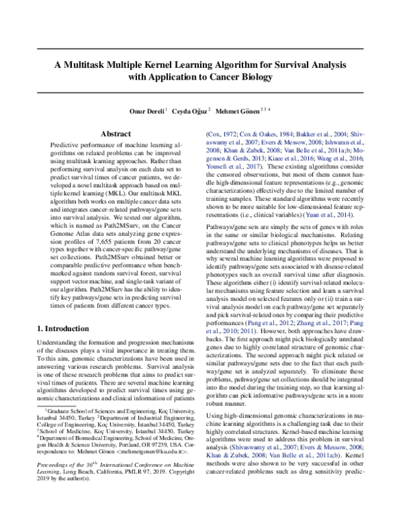
 Ceyda Oguz