Optimal Reserve Prices in Upstream Auctions: Empirical Application on Online Video Advertising Miguel Angel Alcobendas Sheide Chammas Yahoo! Inc. Yahoo! Inc. lisbona@yahoo-inc.com chammas@yahooinc.com ABSTRACT We consider optimal reserve prices in BrightRoll Video Exchange when the inventory opportunity comes from other exchanges (downstream marketplaces). We show that the existence of downstream auctions impacts the optimal floor. Moreover, it renders the classical derivation of the floor set by a monopolist inadequate and suboptimal. We derive the new downstream-corrected reserve price and compare its performance with respect to existing floors and the classical optimal monopoly price. In our application, the downstream-corrected reserve price proves superior to both. The proposed model also deals with data challenges commonly faced by exchanges: limited number of logged bids in an auction, and uncertainty regarding the bidding behavior in other exchanges. The relevance of this study transcends its particular context and is applicable to a wide range of scenarios where sequential auctions exist, and where marketplaces interact with each other. 1. INTRODUCTION The importance of video advertising is growing. According to a PWC report 2015 [1], online video advertising revenue exhibits the fastest growth in internet advertising: rising from $6.32bn in 2014 to a forecasted revenue of $15.39bn in 2019. Using data from BrightRoll Video Exchange, we estimate and test a structural model to compute optimal reserve prices. A reserve price corresponds to the lowest bid that the seller is willing to accept for his item. The novelty of this work is that we set the optimal reserve price in a marketplace (upstream) taking into account that, in order to deliver the video advertisement, the winner of the exchange competes against bidders in a second exchange, called downstream marketplace. The use of several exchanges may help publishers to increase demand and competition for the inventory opportunity, since different marketplaces may have different demand partners. As the reader may anticipate, the inforPermission to make digital or hard copies of all or part of this work for personal or classroom use is granted without fee provided that copies are not made or distributed for profit or commercial advantage and that copies bear this notice and the full citation on the first page. Copyrights for components of this work owned by others than ACM must be honored. Abstracting with credit is permitted. To copy otherwise, or republish, to post on servers or to redistribute to lists, requires prior specific permission and/or a fee. Request permissions from permissions@acm.org. KDD ’16, August 13-17, 2016, San Francisco, CA, USA c 2016 ACM. ISBN 978-1-4503-4232-2/16/08. . . $15.00 DOI: http://dx.doi.org/10.1145/2939672.2939877 Kuang-chih Lee Yahoo! Inc. kclee@yahoo-inc.com mation that an exchange has regarding other marketplaces is limited. Our model accounts for that, as well as, partial knowledge of bids submitted in the own exchange. In this paper, we derive the reserve price, also called floor, that BrightRoll Video Exchange should charge in order to maximize its expected profits considering the existence of a downstream auction. In our analysis, we will assume that Brightroll conducts a second price auction and the downstream exchange uses a first price auction to allocate impressions. From an exchange perspective, video advertising is not very different from allocating static display advertising: the publisher has an inventory opportunity that wants to monetize using an auction conducted by a marketplace. The main difference between the classic banner and video ads is the format: we may have a video ad playing before (pre-roll), during (mid-roll), or after (post-roll) the streaming content. The format affects the bidder’s valuation of the opportunity. In the presence of downstream auctions, the publisher sends an ad-request to a marketplace (downstream). Then, the exchange will send a bid request to several real time bidders (RTB), that may be, for instance, demand aggregators (DSP), advertisers, or other marketplaces (upstream). The upstream marketplace will also auction the opportunity. The winner of the latter exchange will then compete against bids submitted downstream. Finally, the downstream winner will be the one delivering the advertisement. We are not aware of any study quantifying the importance of downstream auctions. However, at BrigthRoll a significant amount of inventory opportunities comes from other exchanges. Given the relevant role of the company on video advertising, we believe that their implications deserve to be studied. We show that, for a given inventory opportunity, the optimal upstream exchange floor is greater than the monopoly reserve price developed by Myerson [8] and Riley and Samuelson [10]. The result is very intuitive: the existence of a downstream exchange makes harder to deliver the video ad, since the upstream winner has to compete against downstream bidders. We use auction theory and statistical tools to overcome data limitations. In particular, we only have information about auctions with bids above the current reserve price, which leads to a left-censored data problem. Moreover, conditional on auctions with bids above the floor, we only know the identity of the winning bidder, its bid, the second highest bid, and the current floor. We do not either have data about auctions conducted downstream, except a dummy variable indicating that the upstream winner also won the downstream auction and delivered the video ad. Due to the large amount of data and expensive computations, we decided to implement the algorithm using Apache Spark, a general-purpose cluster computing system designed to deal with this type of tasks. We measure the impact of the aforementioned classical optimal floors on inventory with and without a downstream exchange. Then, we use experiment data to derive the expected performance of optimal floors with the downstream correction. Our test shows that implementing the classical monopoly reserve price without a correction increases the overall generated revenue on inventory with and without a downstream auction. In the particular case of inventory with BrightRoll Video Exchange as a unique marketplace, the expected revenue lift equals 39%, with a observed revenue increase in 77% of the different types of inventory, also called placements. If we look at the effects of the classical optimal floor set by a monopolist on inventory with downstream auctions, results are mixed: while the overall expected revenue lift with respect to current floors equals 25%, our recommendations only increased revenue in 67% of the analyzed placements. Results improve when we use floors that account for the existence of downstream auctions. In such a case, the expected revenue lift equals 29% and revenue increased in 77% of placements, outperforming the results from the classical optimal monopoly floor. As expected, our recommendations work better when we set floors above the current ones. As previously mentioned, data is left-censored. As a result, we have to infer the distribution of bidders’ valuation using data that is only observed when bids are above current floors. The rest of the paper is organized as follows. Section 2 reviews previous work. Section 3 introduces general aspects of the type of problems that we are trying to solve. Section 4 presents the model and optimality conditions for the reserve price. Section 5 outlines the estimation methodology. Section 6 describes the data and estimate results. Section 7 presents the experiment results. Finally, section 8 concludes. 2. RELATED WORK Reserve prices have been largely studied in auction theory. However, empirical literature is scarce. One of the rare studies was conducted by Ostrovsky and Schwarz [4]. Their paper is one of the first large scale experiments measuring the impact of setting reserve prices for online advertisement. They combine previous work in auction theory by Myerson [8], Riley and Samuelson [10] and Varian [12] to derive optimal floors for sponsored search. Their experiment shows that revenue substantially increases as a result of implementing optimal reserve prices. While they have full information about advertisers bids, we have to face the problem of limited data and sequential auctions. Yuan et al. [13] empirically test several algorithms to set reserve prices. They propose a real-time control function approach to correct reserve prices by using the highest bid. They also test the classical derivation of the optimal monopoly price based on the aforementioned work by Myerson [8] and Riley and Samuelson [10], and two other algorithms based on the regression of the two highest bids. Based on results from their experiment, the proposed control function approach works better than the optimal monopoly floor ap- proach. Due to system requirements, we are not allowed to change the reserve price at impression level, preventing us to test the Yuan et al. [13] approach. In any case, we are concerned about the longterm effects of their proposed algorithm. Having a reserve price that directly depends on the highest bid may give bidders incentives to shade their bids as in first price auctions (see V. Krishna [6]). Authors are aware of this possibility, but due to confounding factors (e.g. holidays at the beginning of the experiment, bidders being not aware of the experiment, ...) they could not show that bidding behavior were not affected by the algorithm. We could neither use the regression based models since we do not observe auction data when the highest bid is below the reserve price. From a theoretical perspective, our paper is related to sequential auctions and auctions with intermediaries. The existing theoretical work assumes that the distribution of the bidders’ valuation and the number of competitors is known at each round of auctions. This is not our case since we do not have much information about what is happening downstream. For instance, McAfee and Vincent [7] derive optimal floors when the auctioneer is able to resell the object in a new auction round if bids are lower than the set floors. Other theoretical studies like Feldman, et al. [5], and Stavrogiannis et al. [11] characterize the equilibrium behavior of the players in an auction with intermediaries. In their models, there exists an exchange (downstream) that sends the bid request to other upstream exchanges (intermediaries). Given a predefined auction mechanism, Feldman et al. [5] focus on the derivation of the profit maximizing reserve price set by the downstream and upstream exchanges, and the optimal fee charged by the intermediary. On the other hand, Stavrogiannis, et al. [11] study the optimal reserve price set by the downstream exchange and the intermediary profits depending on the auction design. 3. 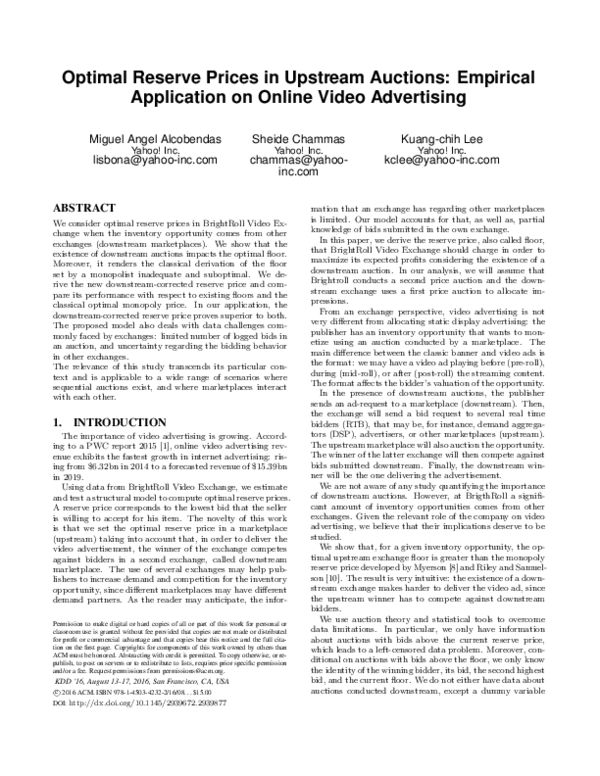BACKGROUND Figure 1 displays the analyzed business model. When a publisher has an inventory opportunity, it sends an advertisement request to a marketplace denoted as Downstream M arketplace, which conducts an auction to allocate the opportunity. Then, the downstream marketplace will send a bid request to several real time bidders (RTB), that may be demand aggregators (DSP), advertisers, or other marketplaces. In Figure 1, we have two real time bidders: dsp1 and an exchange denoted as U pstream M arketplace. Similarly, the upstream marketplace will also conduct an auction to determine the winner and the bid passed to the downstream exchange. In our application the upstream exchange corresponds to BrightRoll Video Exchange. The upstream marketplace is assumed to conduct a second price auction, and the downstream exchange uses a first price auction mechanism to allocate impressions. Both exchanges are able to set reserve prices in order to maximize their expected revenue. In this paper, we focus on the optimal floors set by the upstream exchange. Only if the advertisement is delivered, the winner of the downstream marketplace pays the transaction price, and the exchange and publisher split the generated revenue. As we will see later, the optimality condition to set the upstream reserve price does not depend on fees charged by exchanges. For that reason, we will assume that the downstream marketplace does not charge any fee for conducting the auction. Publisher Inventory Opportunity {dsp3,$6} Downstream MarketPlace {dsp3,$6} = {dsp3,$8*(1-0.25)} {dsp1,$5} Upstream MarketPlace dsp1 {dsp2,$8} {dsp3,$9} dsp3 dsp2 Floor = $4.7 Revenue Share = 25% {dsp4,$4} dsp4 Figure 1: Marketplace Design for a particular inventory opportunity. For each risk neutral bidder i, the valuation of the inventory opportunity, denoted as vi , is assumed to be an independent and identically distributed realization of the random variable V over the interval [0, v̄], which has a cumulative distribution function FV (v) and probability density function fV (v). While the value of the inventory for each potential buyer is private information, the distributions FV (v) and fV (v) are publicly known by participants. For simplicity, we also assume that bidders are not able to switch between marketplaces. In second price auctions with reserve prices, it is a weakly dominant strategy for bidders to bid their own value. The existence of a downstream first-price auction does not change the bidding strategy of participants in the upstream exchange. As a result, truth-telling continues being a dominant strategy. That is, bi = vi for r ≤ vi This is the case where publishers manage the allocation of their inventory using their own marketplace (e.g. Yahoo!, Facebook,...). On the other hand, the upstream marketplace will keep a percentage of the clearing price of the winning bid. As we will explain in detail later on, to ensure that the upstream exchange gets paid, it will keep the corresponding fee before passing the bid to the downstream auction. As an illustration, imagine the scenario depicted in Figure 1. The publisher has an inventory opportunity and sends an ad request to the downstream marketplace. The exchange will send a bid request to the upstream marketplace and dsp1. Then, the upstream marketplace will ask DSPs 2, 3 and 4 to submit a bid for the inventory opportunity. Assume that dsp2 submits a bid that equals 8 dollars eCPM, dsp3 bids 9, and dsp4 bids 4. Only bids above the floor are considered. In this example, the upstream floor is set to $4.7. As a result, the bid submitted by dsp4 is discarded. Among the remaining bids, the winner of the upstream marketplace is dsp3. Since the exchange employs a second price auction mechanism, we use the bid submitted by dsp2, the set floor and the revenue kept by the marketplace to compute the bid passed to the downstream marketplace. The upstream transition price equals $8 and corresponds to the maximum of dsp2 and the floor set at $4.7. Assume that the upstream exchange keeps 25% of the transaction price if bidder dsp3 is able to deliver the advertisement. Given the revenue share, the bid submitted to the downstream marketplace equals $6, which is the result of subtracting 25% from the dsp2 bid (i.e. 6 = 8 ∗ (1 − 0.25)). Consequently, the potential revenue for the upstream marketplace is $2 eCPM. The bid passed to the downstream auction, the tuple {dsp3, $6}, competes with dsp1. Assume that the downstream marketplace sets a floor that is equal to zero and runs a first price auction. Given the auction design and bid submitted by dsp1, dsp3 wins the auction and pays $8. The publisher will keep $6 and the remaining $2 corresponds to the fees charged by the upstream exchange. 4. MODEL In this section we develop the model to estimate the optimal floor that the upstream marketplace should set in order to maximize its expected revenues taking into account the existence of a downstream exchange. In the upstream marketplace, we assume that there exist N potential bidders where bi corresponds to the bid made by i, vi equals the aforementioned valuation of the inventory, and r denotes the reserve price. The proof is very intuitive. Assume that in the upstream marketplace a potential buyer i bids less than his valuation vi . Given such a choice, the bidder would risk losing the inventory opportunity to another interested buyer who bids higher than him, but who has lower valuation. Note that the price paid by the winner is not determined by its own bid but the bid of the nearest opponent. So bidding below vi is not optimal in the upstream auction. This result is reinforced by the existence of a downstream exchange, since bidding below bidder’s valuation increases the probability that a downstream bidder, who values the inventory less than vi , bids slightly higher than the upstream potential buyer. On the other hand, bidding more than bidder’s own valuation increases the chances of winning the upstream and downstream auctions. However, using a similar argument, if the upstream bidder i bids more than vi , he may pay more than the inventory opportunity is worth to him. Since we have ruled out bids both above and below vi , the only option is to bid his own valuation vi . In the presence of a downstream auction, there is no benefit from deviating from truth-telling. Given the ordered bidder’s valuations in the upstream auction v1 > v2 > · · · > vN and knowing that truth-telling is an equilibrium, the bidder with highest valuation v1 wins the upstream auction, and pays, conditional on winning the downstream auction, the maximum between what his nearest opponent is willing to pay v2 and the reserve price r. That is bidder 1 pays w = max{v2 , r} Note that the actual payment is only made if the winner of the upstream auction delivers the advertisement. In order to derive the reserve price, we extend the general formulation proposed by Riley and Samuelson [10] by capturing the effects of introducing a downstream auction. We will follow a similar approach to derive the optimality condition for the reserve price. Since bidders are assumed to be symmetric, we just need to study one buyer (bidder i) to derive his expected payment and the expected revenue of the exchange. Bidder i’s expected profit from participating in the upstream market- Given the upstream marketplace expected profits, in order to find the optimality condition for r to be optimal, we compute the derivative of Πups with respect to r. That is, place equals Π(x, vi ) = vi FV (x)N −1 PD (w̄T (r)) − S(x) where vi is the value of the inventory opportunity for bidder i, x corresponds to bidder i’s bid, and FV (x)N −1 is the probability that bidder i wins the upstream auction (i.e. everybody else bids less than bidder i). PD (w̄T (r)) corresponds to the probability of winning the downstream auction. It depends on w̄T (·) that equals the expected transaction price conditional on having at least one bidder above the reserve price r. As we will discuss in detail later on, w̄T (·) does not directly depend on the reported value but on the known distributions fV and FV . This simplifies the optimization problem. Finally, S(x) is the expected payment given bid x. Since truth-telling is a dominant strategy. The following first-order condition must be satisfied if the bidder wants to maximize his expected gain, i ∂Π(x, vi ) d h FV (x)N −1 PD (w̄T (r)) − S ′ (x) = 0 (1) = vi ∂x dx at x = vi . If the bidder has a valuation equal to the reserve price r, he expects to pay S(r) = rFV (r)N −1 PD (w̄T (r)) (2) Given conditions 1 and 2, bidder i’s expected payment is Z vi S ′ (u)du S(vi ) = rFV (r)N −1 PD (w̄T (r)) + r Z vi i d h = rFV (r)N −1 PD (w̄T (r))+ u FV (u)N −1 PD (w̄T (r)) du du r This expression can be further simplified by integrating by parts as follows, N −1 S(vi ) = vi FV (vi ) PD (w̄T (r)) Z vi N −1 FV (u) PD (w̄T (r))du − r Given bidder i’s expected payment and assuming that there exist N symmetric bidders, we can derive the expected revenue of the upstream exchange and the floor that it should charge in order to maximize its profits. The upstream marketplace expects to receive a percentage of what bidders expect to pay. This revenue share is denoted as rev and treated as given. Since there are N symmetric bidders, the expected revenue of the upstream exchange (Πups ) equals N times the revenue share times the expected payment of each potential buyer (S(·)). That is, Z v̄ S(u)fV (u)du (3) Πups = rev N r Z v̄ h uFV (u)N −1 PD (w̄(r)) = rev N r  Z u N −1 FV (µ) PD (w̄T (r))dµ fV (u)du − r Note that in 3 we compute the expected value of S(·) because the exchange does not know how much each potential buyer values the inventory. It only has information about the distribution of bidders’ valuation. Integrating expression 3 by parts, Z v̄ Πups= rev N PD (w̄T (r)) [uf (u) − 1 + FV (u)] FV (u)N −1 du (4) r ∂Πups =0 ∂r (5) Using equations 4 and 5, the optimality condition is characterized by [rfV (r) − 1 + FV (r)] FV (r)N −1 PD (r) = (6) Z ∂PD (w̄T (r)) v̄ [uf (u) − 1 + F (u)] FV (u)N −1 du ∂r r where the probability of winning in the downstream exchange is assumed to be increasing in r on the support interval [0, v̄]. Using the chain rule, the derivative of the probability of winning the downstream auction with respect to the reserve price equals ∂PD (w̄T ) ∂ w̄T (r) ∂PD (w̄T (r)) = ≥0 ∂r ∂ w̄T ∂r (7) Looking at equation 7, assuming that PD (w̄T (r)) is increasing in r is equivalent to assume that PD (w̄T (r)) is increasing in w̄T , since by definition w̄T increases with r. The reserve price that follows from equation 6 leads to the optimal reserve price and it is denoted as ρ∗c . The following proposition summarizes previous results. Proposition 1: Under the assumptions that bidders’ valuation of the inventory opportunity is an i.i.d. realization of the random variable V , and bidders are risk neutral, the reserve price that maximizes the upstream exchange expected revenue ρ∗c satisfies [ρ∗c fV (ρ∗c ) − 1 + FV (ρ∗c )] FV (ρ∗c )N −1 PD (ρ∗c ) = (8) Z v̄ ∗ ∂PD (w̄T (ρc )) [ufV (u) − 1 + F (u)] FV (u)N −1 du ∂ρ∗c ρ∗ c Note that without downstream auctions, the optimality condition for the monopoly reserve price equals (see Riley and Samuelson [10]) [ρ∗u fV (ρ∗u ) − 1 + FV (ρ∗u )] = 0 (9) where ρ∗u corresponds to the optimal reserve price without downstream correction. Note that, contrary to expression 9, equation 8 depends on the number of competitors and probability of winning the downstream auction. On the other hand, the revenue share kept by the upstream exchange (rev) does not have any impact on the optimal reserve price. Proposition 2: Under the assumptions that bidders’ valuation of the inventory opportunity is an i.i.d. realization of the random variable V , bidders are risk neutral, and the probability of winning the downstream auction is increasing in the reserve price, the reserve price that maximizes the upstream exchange expected revenue ρ∗c is greater than the uncorrected optimal floor ρ∗u . The proof is straightforward. Under the stablished assumptions, the payment of upstream bidders is increasing in r, and the optimal reserve price that maximizes the upstream expected revenue in the presence of a downstream exchange is ρ∗c . As a result, using ρ∗u in equation 6 is not optimal, lowering the expected revenue. Proposition 2 states that, for a given inventory, the corrected optimal floor (ρ∗c ) is greater than the uncorrected one (ρ∗u ). This result is very intuitive: the existence of a downstream auction makes harder to show an impression since the winner of the upstream marketplace has to compete against downstream bidders. As a result, the upstream floor is increasing with downstream competition. That explains why ρ∗c is greater than a reserve price that does not account for the existence of downstream exchanges (ρ∗u ). As we will discuss in detail later on, we will analyze the impact of ρ∗c and ρ∗u using data from BrightRoll Video Exchange. The last part of this section is devoted to further develop the term w̄T , that corresponds to the expected transaction price conditional on having, at least, one bidder above the reserve price. By definition, w̄T equals Z v̄ (10) ufWT (u, r)du w̄T (r) = rPWT (w = r) + r where the first component on the right hand side is the expected payment when there is a single bidder above the reserve price, and the second term equals the expected payment when two or more bids are above the reserve price r. PWT (w = r) corresponds to the probability that the transaction price w is equal to the reserve price r, and fWT (u, r) is the probability distribution function of the transaction price when there exist more than one bid above the reserve price. Both probabilities are conditional on having, at least, one bid above r. That is, the conditional probability for w = r corresponds to   N FV (r)N −1 [1 − FV (r)] PWT (w = r) = 1 − FV (r)N where the numerator indicates the probability that there is a single bid above the reserve price, and the denominator equals the probability that someone bids above the reserve price. As previously discussed, for a particular auction we do not observe all bids. We only have information regarding the highest and the second highest bid as long as they are above the reserve price. As a result, we will use the density function of the second highest bid to compute fWT . That is, the density function of the transaction price conditional on having two or more bidders above the reserve price equals   N (N − 1)FV (u)N −2 [1 − FV (u)]fV (u) fWT (u, r) = (11) 1 − FV (r)N The numerator in 11 corresponds to the density function of the transaction price w when it is equal to the second highest bid. Consequently, it follows the distribution of the second-highest-order statistic from an i.i.d. sample of size N and distribution fV (see Arnold, Balakrishnan, and Nagaraja (1992) [3]). Once again, the denominator equals the probability that there exists at least one bid above the reserve price. After some algebra, it is easy to show that the corresponding derivative with respect to the reserve price equals Z v̄ ∂ w̄T (r) ∂ ∂ ufWT (u, r)du = rPWT (w = r) + ∂r ∂r ∂r r Z v̄ ∂fWT (u, r) ∂PWT (w = r) + u du = PWT (w = r) + r ∂r ∂r r This derivative will be used to compute the optimal reserve price (ρ∗c ) in equation 8. In the next section we discuss how to implement the previous results to get the optimal floor using data from BrightRoll Video Exchange. 5. ESTIMATION In order to compute the optimal floor in equation 8 we need the distribution of bidders’ valuation of the inventory opportunity (fV , FV ), and the expected probability of winning the downstream auction (PD ). This section outlines the procedure to estimate the aforementioned distributions. The BrightRoll Video Exchange data set only contains information about auctions with the highest bid above the reserve price. Consequently, we do not have data about upstream auctions where all bids are below the set floor. The data set includes details about the type of inventory (also called placement), the identity and the bid of the winner in the upstream auction, the transaction price (w) and the current reserve price (r). Regarding downstream marketplaces, we only know which upstream auctions led to an impression in the downstream exchange. Our algorithm takes into account the available information in order to compute the optimal reserve price in the upstream auction when inventory comes from other exchanges. We use a two-step approach to estimate the floor price: firstly, we characterize the distribution of the buyers’ valuation of the inventory (fV and FV ), and estimate the parameters capturing the relationship between the probability of wining downstream and the expected transaction price. In step two, we will use the estimates and expression 8 to compute the optimal reserve price. In step 1, we follow Paarsch and Hong [9] and estimate the parameters of the model using the likelihood function of the transaction price (w). As previously stated, given the ordered bidder’s valuations in the upstream auction v1 > v2 > · · · > vN , w equals w = max{v2 , r} Once again, the actual payment is only made if the winner of the upstream auction delivers the advertisement. When the upstream exchange conducts an auction we may have three possible scenarios: one where all bids are below the reserve price, the case where only one bidder is willing to pay more than the reserve price, and the outcome where two or more bidders submit a bid above the floor. We will combine the probability of each event to construct the probability density function of the transaction price w. The probability that all bidders bid below the reserve price equals P r(w = 0) = FV (r; θ)N where θ corresponds to the vector of parameters defining the shape and scale of the parametric distribution of the bidders’ value of the inventory. When only one potential buyer bids above the reserve price and the rest N − 1 bidders have valuations below it, the probability is equal to P r(w = r) = N FV (r; θ)N −1 [1 − FV (r; θ)] Finally, the corresponding probability density when two or more bidders value the inventory more than the reserve Given the probability density function defined in 13, we can construct the likelihood function as follows L= Q Y fW (wt ; θ|zt ) (14) q=1 Figure 2: Truncated Probability Distribution of W price is fˆW (w, n > 2; θ) = N (N − 1)FV (w; θ)N −2 fV (v; θ) = exp(θ1 )θ2 v θ2 −1 exp(−exp(θ1 )v θ2 ) ×[1 − FV (w; θ)]fV (w; θ) where n is the number of bids above the reserve price. This expression corresponds to the distribution of the transaction price when it is equal to the second highest bid, and it follows the distribution of the second-highest-order statistic from an i.i.d. sample of size N and distribution fV (see Arnold, Balakrishnan, and Nagaraja [3]). Figure 2 displays the truncated density function of the transaction price in the upstream exchange. As previously mentioned, the distribution has three parts: the transaction price w equals zero when the inventory is not allocated, w equals the reserve price when only one potential bidder bids above r, and w follows the distribution fˆW when more than one bidder values the opportunity above r. As a result, the probability density function of w in the presence of a reserve price is:   D0 ∗ fW (w; θ) = FV (r; θ)N (12)   D1 N FV (r; θ)N −1 [1 − FV (r; θ)]  1−D0 −D1 N (N − 1)FV (w; θ)N −2 [1 − FV (w; θ)]fV (w; θ) where D0 and D1 are indicator variables. D0 = 1 if all bids are below the reserve price and 0 otherwise. On the other hand, D1 = 1 if and only if one of the bids is above the reserve price. Since the dataset does not contain information about auctions with the highest bid below r, we use the truncated version of equation 12 (see Amemiya 1985 [2]), fW (w; θ) = N FV (r; θ)N −1 [1 − FV (r; θ)] 1 − FV (r; θ)N !D1 N (N − 1)FV (w; θ)N −2 [1 − FV (w; θ)]fV (w; θ) 1 − FV (r; θ)N where Q corresponds to the total number of auctions conducted for a particular type of inventory. Remember that θ corresponds to the vector of parameters characterizing distributions FV and fV . Since we do not have information about auctions with the highest bid below the current floor, we need a parametric distribution to make out of sample predictions. That is, to obtain the optimal reserve price, we need to evaluate the expected revenues when floors are below the current one. This type of inference cannot be done using nonparametric approaches. However, choosing a parametric form has some risks linked to misspecification that can lead to poor results. We can assume different parametric forms as long as they have positive support. In our application, we use the Weibull family with density function defined as (13) !1−D1 Note that fW does not depend on the probability of winning the downstream auction. This is because upstream bidders have incentive to report their true valuation independently of winning in the downstream exchange. Given the likelihood function in 14, we can estimate the vector of parameters θ by minimizing the negative log likelihood. That is, θ∗ = arg min -log(L) θ (15) In order to compute optimal reserve prices in equation 8, we also need to estimate the relationship between the probability of winning the downstream auction PD , and the expected conditional transaction price w̄T . In this paper, we assume a simple linear relationship between both variables, PD (w̄T ) = γ0 + γ1 w̄T (r) + ǫ (16) where γ0 and γ1 correspond to the intercept and slope respectively. ǫ captures possible measurement errors and unobserved factors for the upstream auction designer. Assuming that ǫ is i.i.d. and it is neither correlated with w̄ nor r, we estimate the parameters using ordinary least squares. If the assumptions hold, the resulting estimates of γ0 and γ1 are unbiased. However, we are aware that some correlation between w̄ and the unobserved part may exists. For instance, the value of the inventory opportunity may depend on the hour of the day or type of user, affecting the probability of winning the downstream auction and the expected upstream transaction price. This omitted variable problem may be solved by using instrumental variables. Further research should be devoted to avoid this confounding problem. Given the parameter estimates, we use the optimality condition 8 to compute the upstream optimal reserve price when we account for the existence of a downstream exchange (ρ∗c ). Similarly, we will use condition 9 when we do not account for the existence of downstream auctions (ρ∗u ). 6. DATA AND ESTIMATE RESULTS We use data provided by BrightRoll Video Exchange and estimate the optimal reserve price for inventory with and without a downstream marketplace. In the case where there is only one exchange managing the ad-request, BrightRoll is the only one deciding which bidder will deliver the advertisement. On the other hand, when there exists a downstream valuation of inventory A (F̆V ) with the Weibull parametric approximation (FV ). Given the aforementioned limitations of the nonparametric approach, the comparison is only possible for the range of observed data. In this particular example, the nonparametric representation is limited to values above the current reserve price set at 2.67 dollars eCPM. In order to compute the nonparametric distribution, we use the definition of cumulative distribution function of the second order statistic F̆W , Placement A Cumulative Distribution Function - Fv 1 ML-Estimated CDF Nonparametric CDF 0.95 0.9 0.85 0.8 F̆W = N ∗ F̆v(N −1) − (N − 1) ∗ F̆vN 0.75 where N is assumed to be known.2 F̆W can be constructed using observed data. Given this information, we just need to find F̆V such that the equality in 17 holds. In the particular case of A, the Weibull and the nonparametric distributions are pretty close. This is not always the case. Given the estimates of the density and cumulative distribution functions, we use ordinary least squares to estimate the parameters that define the relationship between PD and w̄T (equation 16). Further details about how we estimate the equation can be found in Appendix 1. Once all the parameters of the model are estimated, computing reserve prices ρ∗c and ρ∗u follows from equations 8 and 9 respectively. 0.7 0 10 20 30 40 50 Valuation - v Figure 3: Inventory A: ML vs Nonparametric CDF marketplace, we will estimate the reserve price taking into account that the winner of the BrightRoll exchange will compete against other bids in a downstream auction. In such a case, the BrightRoll Exchange will be considered the upstream marketplace. We used 2 weeks data and experimented with inventory with and without downstream auctions. Such an inventory captures a significant amount of revenue for BrightRoll. We studied 71 placements for the case where we only have one exchange, and 30 placements with a downstream marketplace. Due to the large amount of data and expensive computations, we decided to implement the algorithm using Apache Spark, a general-purpose cluster computing system designed to deal with this type of tasks. We estimated the optimal floor for each placement during the first 3 days of the experiment. Then we computed the average of the daily results weighted by the number of adrequests. The resulting inventory floors were used in the A|B test during the remaining days of the experiment. In this paper, we assume that in our training set all downstream exchanges conduct a first price auction and upstream marketplaces use a second price auction. In reality, this is not always the case. For some placements, exchanges work in the opposite way: the downstream uses a second price and the upstream marketplace a first price auction. For this type of inventory, our results can be interpreted as a simulation exercise of the consequences of applying optimal floors if placements used the business model considered in the paper.1 For each of placement, we estimate the distribution of bidders’ valuation using expression 15. As previously discussed, the use of a parametric distribution may have misspecification problems. However, in our application this approach is necessary in order to deal with data limitations. We could test how close the parametric approach is from the nonparametric model, and compare the behavior of different parametric families. However, in this paper we will use the expected lift of our recommended floors with respect to the currently implemented ones in order to asses the success of our model. As an illustration, Figure 3 compares the nonparametric cumulative distribution function of bidder’s 1 We are aware that some bias may exist in the estimates linked to the downstream correction term (PD ). (17) 7. A|B TEST RESULTS We conducted an A|B test in order to assess the impact of recommended floors. For each placement, we randomly split the ad-request traffic in two: 5% of the traffic is randomly selected to be part of the group with the recommended floor (test group), and the rest of the traffic will belong to the control group and use the current reserve price. In order for the reader to understand how we measure the effectiveness of floor recommendations, Table 1 displays two types of inventory which are denoted B and C. While inventory B does not face a downstream auction, the upstream winner of C has to compete against bids from other bidders in the downstream exchange. The F loor column in Table 1 shows the implemented reserve price for the test and control groups, and it is measured in dollars eCPM. The variable Exp indicates if the row corresponds to the test (Exp = 1) or control group (Exp = 0). N b Auctions denotes the number of ad-requests for that particular type of inventory. N b Successf ul indicates the number of adrequests that ends up with a winner in the upstream auction. Column 6 corresponds to the ratio of successful auctions to the total number of ad-requests. As the name indicates, column N b Impressions denotes the total number of shown ads. The difference between the number of impressions and successful auctions is displayed in column 8. Several reasons explain why the number of impressions is different from the number of successful auctions: first, having a winner in the upstream exchange does not guarantee that the bidder is going to win the auction conducted downstream. Second, video advertisement is characterized by having a high fallout rate. That happens when the winner of the ad-request is not able to deliver the advertisement (e.g. due to creative errors or latency problems loading the video). For simplicity, we assume that the fallout rate is independent of the bid made 2 Since we know the identities of the upstream winners, we use the inverse of the Herfindahl index to compute the number of effective competitors N . Inventory B C Floor ($eCPM) 13.41 2.00 7.69 13.33 Exp 1 0 1 0 Nb Auctions 68,872 1,308,445 1,770,254 33,613,967 Nb Successful 60,151 1,194,116 281,262 844,257 Nb Successful / Nb Auctions 87% 91% 16% 2% Nb Impressions 24,021 467,240 18,704 119,933 Nb Impressions/ Nb Successful 40% 39% 7% 14% Revenue Lift 8% 101% Table 1: A|B Output by potential buyers. Finally, the Revenue Lif t denotes the expected revenue lift as a result of implementing the recommended floor. Note that the test and control groups are not directly comparable, since the test group only corresponds to 5% of all ad-requests. For that reason, we standardize the amount using the total number of ad-requests in the test and control groups. If we look at inventory B in Table 1, we propose a 13.41 dollars eCPM reserve price instead of the current one set at $2. As previously noted, the number of auctions assigned to the test group is 5% of the total number of ad-requests. Among these ad-requests, 87% of auctions in the test group are successful. The percentage is lower than the one in the control group (91%). This result is expected, since increasing the floor decreases the probability that an auction clears (i.e. auction with at least one bidder above the floor). If we look at the ratio of impressions to the number of successful auctions, around 40% of successful auctions led to an impression in both groups. After standardizing the revenue, the expected revenue lift as a result of implementing the recommended floor equals 8%. Similar analysis can be done for inventory type C. In this case, we recommend a floor below the current one (7.69 dollars eCPM instead of $13.33). Lowering the floor, the ratio successful to total auctions in the upstream marketplace increases from 2% to 16%. Once again, this result is expected since lowering floors rises the probability that at least one bidder bids higher than the reserve price. In contrast to inventory B, in C the ratio of impressions to number of successful auctions in the test group is half of the control. This is consistent with the existence of downstream auctions. As previously noted, the upstream winner of inventory C has to face the competition from other bids submitted in the downstream auction. Decreasing the reserve price, increases the number of auctions that clears upstream. However, it decreases the bid passed to the downstream exchange, decreasing the probability of winning the downstream auction. This is not the case in auctions of type B, where the ratio of impressions to number of successful auctions is the same for the control and test groups. In placements without downstream exchanges, like inventory B, winners do not face competition from other marketplaces. If this is the case, the only reason that explains that the ratio is lower than one is fully attributed to fallout, that is assumed to be independent of the transaction price. We computed and tested the impact of optimal floors on inventory with and without downstream auctions. Due to business requirements, in the A|B experiment we applied the floor resulting from expression 9 and denoted as ρ∗u . We did not directly applied the correction for the existence of a downstream exchange as appearing in equation 8 (ρ∗c ). Instead, we use the data resulting from the experiment and the predicted downstream winning probability to evaluate the optimal floor with the downstream correction. Further details about how we evaluate the effects of the corrected optimal floors can be found in Appendix 2. Table 2 displays the impact of implementing the new floors. Results are aggregated for confidentiality reasons. The first column describes the type of inventory: the first row corresponds to auctions without a downstream exchange. The second row describes the impact of implementing uncorrected optimal floors on inventory with downstream auctions (ρ∗u ). Finally, the third row describes auctions with a downstream marketplace and corrected optimal reserve price ρ∗c . Column N b P lacements captures the number of placements in the experiment. We tested optimal floors in 71 placements without downstream auctions. Similarly, we studied the impact of changing floors in 30 placements with a downstream marketplace. The third column describes the percentage of placements that lead to a lift in revenues. This is one of the main indicators to assess the validity of our predictions. For the case of placements without downstream auctions, 77% of our recommended floors (one for each placement) led to an increase in revenue. Performance decreases when applying the uncorrected optimal floor ρ∗u to placements with downstream auctions. In this case, 67% of the recommendations led to an increase in revenues. The last row displays the effects of using ρ∗c . In this situation, 77% of the recommended floors led to an increase in revenue. The latter result indicates that the corrected floor ρ∗c outperforms the standard formulation of optimal monopoly floors without the correction (ρ∗u ). Placements are very heterogeneous. They may differ in terms of publisher, targeted device, number of ad-requests, etc. Consequently, the effects of implementing optimal floors at placement level can be very different. For that reason, we decided to report the overall revenue lift and not the average across placements. The last column in Table 2 shows the expected revenue lift as a result of the recommendations. This indicator is computed using the total revenue generated across all analyzed placements in the control group and the standardized revenue of the test group. Implementing optimal reserve prices increases revenue. In the case of placements without downstream marketplaces, the expected revenue lift equals 39%. Consistent with the theoretical findings, the optimal reserve price with downstream correction outperforms the uncorrected monopoly price: 29% revenue lift when using ρ∗c vs 25% when testing ρ∗u . Note that the revenue lift as a result of new floors is lower in exchanges with downstream auctions than without. Differences between both types of inventory may be one of the reasons that explains such as discrepancy. As discussed in the introduction, the use of several exchanges may help publishers to increase competition for the inventory, decreasing the effectiveness of floors. Table 3 disaggregates previous results by type of recom- Type of Placement Nb Placements No Downstream Auction (ρ∗u ) Downstream Auction: No Correction (ρ∗u ) Downstream Auction: Correction (ρ∗c ) 71 30 30 Placements with Positive Revenue Lift (%) 77% 67% 77% Expected Revenue Lift (%) 39% 25% 29% Table 2: Aggregated A|B Test Results Type of Placement No Downstream Auction (ρ∗u ) - Above Current Floor - Below Current Floor Downstream Auction: No Correction (ρ∗u ) - Above Current Floor - Below Current Floor Downstream Auction: Correction (ρ∗c ) - Above Current Floor - Below Current Floor Nb Placements Placements with Positive Revenue Lift (%) Expected Revenue Lift (%) 24 47 88% 72% 38% 40% 9 21 100% 52% 92% 11% 13 17 100% 71% 88% 22% Table 3: A|B Test Results by Recommendation Type mendation: above and below the current reserve price. For inventory without downstream auctions, 24 out of 71 placements have a recommended floor above the current one, and 47 out of 71 have a lower recommendation. The performance of the recommended floors is linked to the available data. Remember that we only have data about auctions where the highest bid is above the reserve price. As a result, we have to infer the shape of the distribution of buyers’ valuation for values below the current floor, decreasing the performance of recommendations. As expected, the model behaves better when we recommend above: 88% of recommendations above the current floor led to a positive revenue lift, and 72% for recommendations below the current reserve price. When analyzing the impact of uncorrected floors (ρ∗u ) on inventory with a downstream auction, all recommended floors above the current ones led to an increase in revenue. On the other hand, only 52% of recommendations below the current floor led to a rise in revenue. Finally, the last three rows in Table 3 displays the performance of recommended floors when we correct for the existence of a downstream auction (ρ∗c ). We can see that we improved revenue in 100% of placements where we make recommendations above the current reserve price. On the other hand, effectiveness decreases to 71% when we recommend below. Once again, in the presence of other exchanges ρ∗c performs better than ρ∗u . 8. CONCLUSION In this paper, we derive the reserve price that BrightRoll Video Exchange should charge in order to maximize its expected profits when inventory opportunities come from other marketplaces. We prove that the classical approach to derive the monopoly reserve price is suboptimal. Consistent with the theoretical findings, in our application the downstreamcorrected reserve price increases the expected revenue of the marketplace with respect to the current floor and the classical derivation of the optimal monopoly price. The proposed algorithm also deals with data challenges commonly faced by exchanges: limited number of logged bids per auction, and limited information about inventory coming from other exchanges. The model can easily accommodate features. As a re- sult, we can derive different floors depending on supply and demand characteristics (e.g. hour of the day, user characteristics, video format,...). Moreover, the relevance of this study transcends its particular context and is applicable to a wide range of scenarios where sequential auctions exist and where marketplaces interact with each other. Finally, further research can be devoted to analyze the endogeneity problem when deriving the relationship between the probability of winning downstream and the expected transaction price. 9. REFERENCES [1] Global entertainment and media outlook 2015-2019. http://www.pwc.com/outlook. [2] T. Amemiya. Advanced econometrics. In Cambridge, Massachusetts: Harvard University Press, 1985. [3] B. C. Arnold, N. Balakrishnan, and H. N. Nagaraja. A first course in order statistics. In New York: John Wiley & Sons, 1992. [4] B. Edelman, M. Ostrovsky, and M. Schwarz. Internet advertising and the generalized second price auction: Selling billions of dollars worth of keywords. National Bureau of Economic Research, 2005. [5] J. Feldman, V. Mirrokni, S. Muthukrishnan, and M. M. Pai. Auctions with intermediaries: extended abstract. In the ACM EC, 2010. [6] V. Krishna. Auction theory. In Massachusetts: Elsevier Academic Press, 2nd edition, 2010. [7] R. P. McAfee and D. Vincent. Sequentially optimal auctions. Games and Economic Behavior, 18(2):246–276, 1997. [8] R. B. Myerson. Optimal auction design. Mathematics of operations research, 6(1):58–73, 1981. [9] H. J. Paarsch and H. Hong. An introduction to the structural econometrics of auction data. In Cambridge, Massachusetts: MIT Press, 1st edition, 2006. [10] J. G. Riley and W. F. Samuelson. Optimal auctions. The American Economic Review, pages 381–392, 1981. [11] L. C. Stavrogiannis, E. H. Gerding, and M. Polukarov. Auction mechanisms for demand-side intermediaries in online advertising exchanges. In the 13th international conference on autonomous agents and multiagent systems. AAMAS, 2014. [12] H. R. Varian. Position auctions. International Journal of Industrial Organization, 25(6):1163–1178, 2007. [13] S. Yuan, J. Wang, B. Chen, P. Mason, and S. Seljan. An empirical study of reserve price optimisation in real-time bidding. In Proceedings of the 20th ACM SIGKDD international conference on Knowledge discovery and data mining. ACM, 2014. 10. 10.1 APPENDIX Appendix 1: Estimation of the Winning Downstream Auction Probability This section includes further details about the estimation of PD (w̄T ) in equation 16. In order to estimate δ0 and δ1 we first need to construct the dependent variable PD and the covariate w̄T (r). We trim the dataset discarding auctions within the 4th quantile ordered by the highest bid. As a result, the remaining data set only contains auctions with a highest bid between the reserve price and the 3rd quantile. Then we select twenty equidistant cutoff points. For each cutoff, we compute the revenue and the ratio of impressions to number of successful auctions resulting from auctions with a highest bid greater than the cutoff point. Each cutoff point is like imposing a reserve price, since auctions below each point do not clear. As a result, we will have twenty {PD (w̄T )l , w̄T l } for l ∈ {1, ..., 20} pairs. Given the resulting pairs, we will use ordinary least squares to have an estimate of δ0 and δ1 . 10.2 Appendix 2: Estimation of the Winning Downstream Auction Probability Evaluated at the Optimal Floor For each tested inventory with downstream auctions, we use equations 8 and 16 to compute the optimal reserve price ρ∗c and the predicted probability of showing the impression evaluated at the optimal floor (PD (ρ∗c )). For a given inventory, the corrected optimal floor ρ∗c is greater than the uncorrected one ρ∗u . This result allows us to use data from the test group to evaluate the performance of PD (ρ∗c ). We have information about all auctions that successfully cleared even the ones that did not lead to an impression. From the model, we are able to compute the floor with downstream correction ρ∗c and estimate the probability of winning the downstream auction for that particular floor PD (w̄T (ρ∗c )). In order to compute the expected revenue as a result of imposing the corrected optimal floor ρ∗c , we use the expression 6, the parameter estimates resulting from minimizing equation 15, and estimates from equation 16. We also need to estimate the number of impressions resulting from increasing the probability of winning the downstream auction. Using the test group data, we remove successful auctions with the highest bid below ρ∗c (Successf ulc ). We sum the total number of impressions from the trimmed dataset (Impressionsc ). Using expression 10 we compute the expected transaction price given ρ∗c . Given w̄T (ρ∗c ) and using equation 16 and its corresponding estimates, we compute the expected probability of winning the downstream auction P̂D (w̄T (ρ∗c )). We use P̂D (w̄(ρ∗c )), Impressionsc , and successf ulc , to find the extra number of impressions x resulting from increasing the probability of winning downstream as follows, P̂D (w̄(ρ∗c )) = Impressionsc + x Successf ulc (18) Once we obtain x, we can compute the corresponding revenue. While the revenue generated from Impressionsc is easy to compute, the revenue from the new impressions (x) is trickier. The transaction price for impressions x will be equal to the floor with correction ρ∗c . The argument here is as follows: if the new x impressions clear, it must be as a result of increasing the floor. So the clearing price will be ρ∗c . For instance, imagine that the ratio of impressions to number of successful auctions for the corrected floor equals 0.14 (i.e. P̂D (w̄(ρ∗c )) = 0.14). We know that we have 1,000 successful auctions (i.e. successf ulc = 1000), and 100 impressions that qualify with the new floor (i.e. Impressionsc = 100). Then the number of new impressions (x) clearing at the new floor is 40, and the transaction price of each of these extra impressions equals the aforementioned corrected floor ρ∗c .