arXiv:physics/0207067v3 [physics.gen-ph] 9 Jan 2006
A More Rational and Perfect Scheme for C, P, T Transformations
as well as C, T and CP Violations in the Regularization and
Renormalization Processes of High Order Perturbations
Mei Xiaochun
(Department of Physics, Fuzhou University, Fuzhou, 350025, China, E-mail:mxc001@163.com)
Abstracts According to the current transformation theory in particle physics, after time reversal, the
creation operator of a particle is still a creation operator and the annihilation operator of a particle is still
an annihilation operator. This kind of definition is improper. In interaction processes, creation operator
should become annihilation operator and annihilation operator should become creation operator after time
reversal. There also exist some problems in the current P and C transformations. A more rational and
perfect scheme for C, P, T transformations is advanced. In new scheme, the separate C, P, T transformations of transition probabilities are completely the same as the current theory when the regularizations and
renormalizations of high order processes are not considered. Under the united CP T transformation, the
Hamiltonians of strong, weak and electromagnetic interactions are invariable with a completely symmetrical
form CP T H(x)(CP T )−1 = H(x). On the other hand, according to new scheme, the propagation functions
of Femions would change a negative sign, while the propagation functions of bosons is unchanged. In this
way, when mass renormalization is considered in the high order processes, new T, C violation and CP violation would be caused. Meanwhile, the regularization and renormalization of the third order vertex angle
processes would also violate T, C and CP symmetries in new scheme. But the united CP T symmetry still
holds in high order renormalization processes. It leads to the result that positive and negative electrons
have different anomalous magnetic moments. The Compton scattering experiment and the measurements of
anomalous magnetic moments of positive and negative electrons are suggested to verify the existence of C
violation in the high order processes. The result can be used to explain the problem of reversibility paradox
in the non-equilibrium evolution processes of macro-systems, as well as the problem of positive and antimaterial’s asymmetry in current university. Meanwhile, in new scheme, time reversal operator is not an
anti-Hermitian operator again so that the basic demand of quantum mechanics can be satisfied. The parities
of transverse, longitudinal and scalar photons also become identical. So new scheme is more effective and
rational with more perfect symmetry comparing with the current scheme.
PACS number: 11.30, 11.30.Qc, 11.10.Gh
Key words: Quantum theory of field, Symmetry, C, P, T Transformations, C, T Violations, CP Violation,
Regularization, Renormalization, Anomalous magnetic moment
1.Introduction
According to the current transformation theory in particle physics, after time reversal, the creation
operator of a particle is still a creation operator and the annihilation operator of a particle is still an
annihilation operator. This kind of definition can’t coincide with practical situations. In interaction process,
particle’s creation operator should become annihilation operator and annihilation operator should become
creation operator after time reversal. So the current theory of time reversal should be reformed. According
to new definition, particle’s creation and annihilation operators exchange each after time reversal. In this
way, the propagation functions of fermions change a negative sign while the propagation functions of bosons
are unchanged under time reversal. For the strong and electromagnetic interactions when regularization and
renormalization are not considered, the transition probability densities keep unchanged under time reversal.
But in some weak interaction processes just as K 0 and B 0 meson’s decays, time reversal symmetry is also
∗
6= Ujk .
violated owing to the fact that same CKM matrix elements are complex with Ujk
It is also proved that according to new scheme, the regularization and renormalization processes of some
high order perturbations would cause C, T and CP violations. These results can be used to explain the
irreversibility paradox problem of time reversal in non-equilibrium evaluation processes of macro-systems.
On the other hand, in the current theory of P transformation, the parity of transverse and longitudinal
photons is defined as −1 but the parity of scalar photons is defined as +1. This is inconsistent. In the current
theory of C transformation, the transformation relations between spinor positive and anti-particles are
defined as ψc = γ2 γ4 ψ̄ τ and ψ̄c = ψ τ γ2 γ4 . However, in the quantum theory of field, we define ψ = ψ (+) +ψ (−)
and ψ̄ = ψ̄ (+) + ψ̄ (−) . The operators of second quantization ψ and ψ̄ have contained both the component
of positive particles ψ (−) and ψ̄ (+) as well as the component of anti-particles ψ (+) and ψ̄ (−) . It is improper
to regard ψ and ψ̄ as the wave function of positive particles again. Similarly, after C transformation,
�ψc and ψ̄c also contain the both components of positive particles and anti-particles ψ (+) and ψ̄ (−) . It is
also improper to regard ψc and ψ̄c as the wave function of anti-particles again. The real meaning of C
transformation in the quantum theory of field should be that in the coordinate space the creation operator
(+)
(+)
ψ̄s (x) of spinor positive particle exchange with the creation operator ψs (x) of spinor anti-particle. The
(−)
(−)
annihilation operator ψs (x) of spinor positive particle exchanges with the annihilation operatorψ̄s (x) of
spinor anti-particle. The result leads to that the propagation function of fermions also changes a negative
sign under C, while the propagation function of boson is unchanged. For the strong and electromagnetic
interaction processes when regularization and renormalization are not considered, transition probabilities
keep unchanged under new C transformation. Meanwhile, in some processes of weak interaction such as
K 0 and B 0 meson’s decays, CP and T symmetries are violated simultaneously and both violations are
just complementary. That is to say when the regularization and renormalization are not considered, the
calculation results of transition probabilities are completely the same as that in the current theory under
new C, P transformations.
However, when regularization and renormalizations are considered, new C, T violation and CP violation
would be caused in some processes of strong, weak and electromagnetic interactions. It leads to that positive
and negative electrons have different anomalous magnetic moments. The Compton scattering experiment
and the measurements of anomalous magnetic moments of positive electrons are suggested to verify the
existence of C violation in the high order renormalization processes. The results can be used to explain the
asymmetry problem of positive and anti-material in our university at present.
In this way, a more rational C, P, T transformation can be achieved. The Hamiltonians of strong, weak
and electromagnetic interactions are unchanged under united CP T transformation with a completely symmetrical form CP T H(x)(CP T )−1 = H(x) in new scheme, even though the regularizations and renormalizations of high order processes are considered. Comparing with the result of current theory with
CP T H(x)(CP T )−1 = H+ (−x), new scheme is more symmetrical and effective comparing with the current scheme. Meanwhile, time reversal operator is not an anti-Hermitian operator again so that the basic
demand of quantum mechanics can be satisfied, and the parities of transverse, longitudinal and scalar photons also become identical in new scheme.
2. T Transformation
In quantum mechanics, if we suppose that the Hamiltonian is invariable under time reversal with relation
T H(~x, t)T −1 = H(~x, t), the form of Schrodinger’s equation would be unchanged, but wave functions would
become its complex conjugation with T ψ(~x, t) = ψ ∗ (~x, t). It is just in this meaning, we say that the processes
described by the Schrodinger’s equation are unchanged under time reversal. It should be noted that in the
processes described by the Schrodinger’s equation, there exist no particle’s creation and annihilation in
general. The phenomena of particle’s creation and annihilation should be described by the quantum theory
of field. In the quantum theory of field, scalar field ϕ, electromagnetic field Aµ and spinor field ψ are regarded
as operators. There are two schemes for time reversal transformations in current particle physics. In the
first scheme, the T transformations of ϕ, Aµ and ψ are defined individually as below
T ϕ(~x, t)T −1 = ϕ(~x, −t)
T Aµ (~x, t)T −1 = −Aµ (~x, t)
T ψ(~x, t)T −1 = T̃ ψ(~x, −t) = iγ1 γ3 ψ(~x, −t)
(1)
(2)
Where T̃ = iγ1 γ3 is a matrix. It is obvious that the time reversal definition shown in Eqs.(10) and (2) are
different from that in quantum mechanics with T ψ(~x, t) = ψ ∗ (~x, −t). Because ϕ, Aµ and ψ are regarded
as operators in the quantum theory of field, not to be probability amplitudes, the differences seem to be
allowed. By the definitions above, it can be proved that the Hamiltonian of electromagnetic interaction
H(~x, t) = −
ie
Aµ (~x, t)[ψ̄(~x, t)γµ ψ(~x, t) − ψ τ (~x, t)γµτ ψ̄ τ (~x, t)]
2
(3)
satisfies following transformation relation
T H(~x, t)T −1 = H(~x, −t)
(4)
The result shows that thought the Hamiltonian of electromagnetic interaction in particle physics is not
invariable, the calculation of transition probability in light of Eq.(4) in momentum space is still unchanged
under time reversal. Also in this meaning, we say that the interaction processes with particle’s creations
and annihilations is symmetrical under time reversal.
�In order to satisfy Eq.(2), in the current theory, T transformation of quantized spinor field ψ(~x, t) is
carried out according to following procedure (1) . Let ψ(~x, t) = ψ (−) (~x, t) + ψ (+) (~x, t) with
r
r
X m
X m
(−)
i(~
p·~
x−Et)
(+)
ψ (~x, t) =
us (~
p)bs (~
p)e
ψ (~x, t) =
νs (~
p)d+
p)e−i(~p·~x−Et)
(5)
s (~
E
E
p
~,s
p
~,s
Because T̃ is only a matrix, we have
r
X m
[T̃ us (~
p)bs (~
p)ei(~p·~x+Et) + T̃ νs (~
p)d+
p)e−i(~p·~x+Et)
T̃ ψ(~x, −t) =
s (~
E
(6)
p
~,s
It can be proved to have following relations
(1)
T̃ us (~
p) = iγ1 γ3 us (~
p) = ηu u∗s (−~
p)
T̃ νs (~
p) = iγ1 γ3 νs (~
p) = ην νs∗ (−~
p)
(7)
Take ηm = ην = 1 for convenience, Eq.(6) becomes
r
X m
T̃ ψ(~x, −t) =
[u∗ (−~
p)bs (~
p)ei(~p·~x+Et) + νs∗ (−~
p)d+
p)e−i(~p·~x+Et) ]
s (~
E s
p
~,s
=
X
p
~,s
r
m ∗
[u (~
p)bs (−~
p)e−i(~p·~x−Et) + νs∗ (~
p)d+
p)ei(~p·~x−Et) ]
s (−~
E s
(8)
One the other hand, in the current theory, T is an anti-Hermitian operator with nature. That is to say, wave
functions are transformed into their complex conjugate functions after time reversal. So we have
r
X m
−1
[u∗ (~
p)T bs (~
p)T −1 e−i(~p·~x−Et) + νs∗ (~
p)T d+
p)T −1 ei(~p·~x−Et) ]
(9)
T ψ(~x, t)T =
s (~
E s
p
~,s
Comparing Eq.(8) with (9), we obtain
T bs (~
p)T −1 = bs (−~
p)
T d+
p)T −1 = d+
p)
s (~
s (−~
(10)
Eq.(10) shows that creation operator is still creation operator, and annihilation operator is still annihilation
operator after time reversal. Though it seams rational for free particles without creation and annihilation, it is
improper for processes to exist interaction between particles. In practical interaction processes with particle’s
creations and annihilations, creation operator should become annihilation operator and annihilation operator
should become creation operator after time reversal. So in interaction processes, the rational definitions of
time reversal transformations of creation and annihilation operators should be
T bs (~
p)T −1 = b+
p)
s (−~
T d+
p)T −1 = ds (−~
p)
s (~
Let T ψ(~x, t)T −1 = ψT (~x, t), x̃ = (~x, −t), we should have in coordinate space
r
r
X m
X m
ip·x
T
(+)
(−)
us (~
p)bs (p)e
→ ψ̄s (x̃) =
ūs (−~
p)b+
p)e−ip·x
ψs (x) =
s (−~
E
E
=
X
p
~
(12)
p
~
p
~
ψs(+) (x)
(11)
r
X
m
−ip·x
νs (~
p)d+
→T ψ̄s(−) (x̃) =
s (p)e
E
p
~
(−)
r
m
ν̄s (−~
p)ds (−~
p)eip·x
E
(13)
(+)
The formulas indicate that the operator ψs (x) to annihilate a positive particle becomes the operator ψ̄s (x̃)
(+)
(−)
to create a positive particle, and the operator ψ̄s (x) to create an anti-particle becomes the operator ψs (x̃)
to annihilate an anti-particle in coordinate space after time reversal. The same problems exist in the time
reversals of scalar field ϕ, electromagnetic field Aµ when there exist particle’s creations and annihilations.
The same problems also exist in the second scheme of time reversal, i.e. the so-called Winger scheme (2) ,
but it is unnecessary for us to discuss it any more here. As shown below, based on the correct definitions of
creation and annihilation operator’s time reversals, a really rational and more perfect time reversal theory
�can be achieved.The following points can be regarded as the foundational natures of time reversal in particle
physics.
1.Let t → −t, p~ → −~
p in wave functions and other functions to describe micro-particles.
2.Particle’s creation and annihilation operators exchange each other.
3.The wave functions of spinor particles in momentum space are transformed into their conjugate forms.
The concrete transformations are discussed below. For free scalar field ϕ(~x, t) = Aei(~p·~x−Et) , let t → −t,
~p → −~
p after time reversal, we have
T ϕ(~x, t) = Ae−i(~p·~x−Et) = ϕ∗ (~x, t) 6= ϕ(~x, −t)
(14)
The wave function is changed into its complex conjugate form according to new scheme. But it is not the
same as the present result shown in Eq.(1). A more serious problem is that if we only let t → −t but keep
~p unchanged under time reversal as done in current scheme, we have
T ϕ(~x, t) = Aei(~p·~x+Et) = ϕ(~x, −t)
(15)
It means that retarded wave would become advanced wave. This is impossible, forbidden by the law of
causation. For free and real quantized scalar field ϕ(~x, t) = ϕ(+) (~x, t) + ϕ(−) (~x, t)
ϕ(+) (x) =
1
(2π)3/2
Z
p
~=+∞
p
~=−∞
d3 ~
p
√ a+ (~
p)e−i(~p·~x−Et)
2E
ϕ(−) (x) =
1
(2π)3/2
Z
p
~=+∞
p
~=−∞
d3 p~
√ a(~
p)ei(~p·~x−Et)
2E
(16)
we have
T a+ (~
p)T −1 = ηa(−~
p)
T a(~
p)T −1 = η + a+ (−~
p)
(17)
Take η = η + = 1 for simplification and let t → −t, ~p → −~
p after time reversal, we get
(+)
Tϕ
(~x, t)T
−1
1
=−
(2π)3/2
Z
p
~=−∞
p
~=+∞
d3 p~
√ a(−~
p)ei(~p·~x−Et)
2E
(18)
Let −~
p → p~ again, the formula above becomes
T ϕ(+) (~x, t)T −1 =
1
(2π)3/2
Z
p
~=+∞
p
~=−∞
d3 p~
√ a(~
p)ei(−~p·~x−Et) = ϕ(−) (−~x, t)
2E
(19)
Similarly, we have T ϕ(−) (~x, t)T −1 = ϕ(+) (−~x, t). By writing x̄ = (−~x, t) in later discussions, the time
reversal of quantized real scalar field is
T ϕ(x)T −1 = T ϕ(+) (x)T −1 + T ϕ(−) (x)T −1 = ϕ(−) (x̄) + ϕ(+) (x̄) = ϕ(x̄)
(20)
It seams that time reversal becomes space coordinate reversal with ~x → −~x. The result is equivalent to let
~ → −~
p
p at the vertex of the Feynman diagram. This just embodies the practical significance of time reversal.
As shown below, it does not affect the calculation result of transition probability density. So according to
this paper, when there exist particle’s creations and annihilations in interaction processes, time reversal
operator would not be an anti- Hermiltian one again.
For complex scalar fields ϕ(x) = ϕ(+) (x) + ϕ(−) (x), ϕ+ (x) = ϕ+(+) (x) + ϕ+(−) (x)
Z
Z
1
1
d3 p~ +
d3 p~
+(+)
−ip·x
+(−)
√
√
ϕ
(x) =
a
(~
p
)e
ϕ
(x)
=
b(~
p)eip·x
(21)
(2π)3/2
(2π)3/2
2E
2E
Z
Z
1
d3 ~
p +
d3 p~
1
−ip·x
(−)
(+)
√
√
b
(~
p
)e
ϕ
(~
x
,
t)
=
a(~
p)eip·x
(22)
ϕ (x) =
3/2
(2π)3/2
(2π)
2E
2E
According to new scheme, we have T a+ (~
p)T −1 = a(−~
p), T b+ (~
p)T −1 = b(−~
p) and
T ϕ+(+) (x)T −1 = ϕ(−) (x̄)
T ϕ(+) (x)T −1 = ϕ+(−) (x̄)
(23)
T ϕ+ (x)T −1 = ϕ(x̄)
(24)
So we get at last
T ϕ(x)T −1 = ϕ+ (x̄)
�The time reversals of commutation relations between creation and annihilation operators become
T [a(~
p1 ), a+ (~
p2 )]T −1 = [a+ (−~
p1 ), a(−~
p2 )] = −[a(−~
p2 ), a+ (−~
p1 )] = −δ 3 (~
p1 − p~2 )
(25)
T [b(~
p1 ), b+ (~
p2 )]T −1 = [b+ (−~
p1 ), b(−~
p2 )] = −[b(−~
p2 ), b+ (−~
p1 )] = −δ 3 (~
p1 − p~2 )
(26)
T [ϕ(−) (x1 ), ϕ+(+) (x2 )]T −1 = [ϕ+(+) (x̄1 ), ϕ(−) (x̄2 )] = −[ϕ(−) (x̄2 ), ϕ+(+) (x̄1 )]
(27)
Similarly, the time reversals of commutation relations between field operators become
(+)
T [ϕ
+(−)
(x1 ), ϕ
(x2 )]T
−1
+(−)
= [ϕ
(+)
(x̄1 ), ϕ
(+)
(x̄2 )] = −[ϕ
+(−)
(x2 ), ϕ
(x1 )]
(28)
There is a difference of negative sign on the right side of the formulas comparing with the current result.
In fact, it is easy to prove that the commutation relation between coordinate and momentum in quantum
mechanics would change a negative sign after time reversal. From the original definition of time reversal,
we can directly get T [x̂, p̂]T −1 = −[x̂, p̂] = −i. But in current theory of time reversal, it is artificially
supposed that commutation relation between coordinate and momentum is unchanged under time reversal,
i.e., T [x̂, p̂]T −1 = T iT −1, or −[x̂, p̂] = −i = T iT −1. From the result, time reversal operator T is considered as
an anti-Hermiltian operator. However, in principle, the operators of quantum mechanics should be Hermitian
operators. Anti-Hermitian operators are meaningless. Therefore, it is unnecessary for us to consider time
reversal operator as anti-Hermitian one generally. We should decide time reversal transformations of physical
quantities in light of practical situation or original nature of time reversal processes. Though in same special
cases we just have T α = α∗ , but this relation has no universal meaning.
The time reversal transformations of propagation functions are discussed below. The definition of propagation function of complex scalar field is
∆F (x1 − x2 ) = θ(t1 − t2 )[ϕ(−) (x1 ), ϕ+(+) (x2 )] + θ(t2 − t1 )[ϕ+(−) (x2 ), ϕ(+) (x1 )]
Z +∞
d4 p
i
eip·(x1 −x2 )
∆F (x1 − x2 ) = −
(2π)4 −∞ p2 + m2
(29)
(30)
The meaning of Eq.(29) is that when t1 > t2 , only the first item acts and a positive meson is created at
x2 point. Then the meson is annihilated when it reaches x1 point. When t2 > t1 , only the second item
acts and an anti-meson is created at point x1 . Then the anti-meson is annihilated when it reaches x2 point.
According to new scheme, by using Eq.(27) and (28), we have
T ∆F (x1 − x2 )T −1 = −T θ(t1 − t2 )T −1 [ϕ(−) (x̄2 ), ϕ+(+) (x̄1 )] − T θ(t2 − t1 )T −1 [ϕ+(−) (x̄1 ), ϕ(+) (x̄2 )]
(31)
Because T 2 ∼ 1, T ∼ ±1, we have T θ(t1 − t2 )T −1 = ±θ(t2 − t1 ). If taking T θ(t1 − t2 )T −1 = −θ(t2 − t1 ), we
have
T ∆F (x1 − x2 )T −1 = θ(t2 − t1 )[ϕ(−) (x̄2 ), ϕ+(+) (x̄1 )] + θ(t1 − t2 )[ϕ+(−) (x̄1 ), ϕ(+) (x̄2 )]
(32)
It is equal to let x1 → x̄2 , x2 → x̄1 on the right side of Eq.(29), means that when t2 > t1 , only the first item
acts and a positive meson is create at x1 point. Then the meson is annihilated when it reaches x2 point.
When t1 > t2 , only the second item acts and an anti-meson is created at point x2 . Then the anti-meson is
annihilated when it reaches x1 point. The result just coincides with the practical processes of time reversal.
So let x1 → x̄2 , x2 → x̄1 on the right side of Eq.(30), we obtain
Z +∞
i
d4 p
T ∆F (x1 − x2 )T −1 = −
eip·(x̄2 −x̄1 ) = ∆F (x̄2 − x̄1 )
(33)
(2π)4 −∞ p2 + m2
Because p · (x̄2 − x̄1 ) = −~
p · (~x2 − ~x1 ) − p0 (t2 − t1 ) = p~ · (~x1 − ~x2 ) + p0 (t1 − t2 ), the formula can also be
written as
Z +∞
i
d4 p
−1
T ∆F (x1 − x2 )T = −
ei[~p·(~x1 −~x2 )+p0 (t1 −t2 )]
(34)
(2π)4 −∞ p2 + m2
The integral above is unchanged by substitution p0 → −p0 . So we can obtain Eq.(30) from Eq.(34) by
substitution p0 → −p0 , showing that the propagation function of scalar fields is unchanged under time
reversal. In fact, we can also let t → −t, p~ → −~
p directly on the light side of Eq.(30) to get the time reversal
of propagation function of complex scalar fieldthen let p → −p again to prove the time reversal invariability
of scalar field’s propagation function. If taking T θ(t1 − t2 )T −1 = θ(t2 − t1 ), we would get
Z +∞
d4 p
i
ei[~p·(~x1 −~x2 )−p0 (t1 −t2 )]
(35)
T ∆F (x1 − x2 )T −1 =
(2π)4 −∞ p2 + m2
�There exist the difference of a negative sign comparing with Eq.(30), means that the propagation function
of scalar fields reverse its propagation direction under time reversal. This is, of course, improper. Therefore,
according to the new scheme in the paper, the time reversal of step function θ(t) should be defined as
θ(t1 − t2 ) = {10
t1 >t2
T
t1 <t2 →
T θ(t1 − t2 )T −1 = −θ(t2 − t1 ) = {−1
0
For free quantized electromagnetic field Aµ (x) =
Aσ(+)
(x) =
µ
Aµσ(−) (x) =
1
(2π)3/2
+∞
Z
1
(2π)3/2
P4
−∞
Z
σ(+)
σ=1
Aµ
(x) +
P4
σ=1
σ(−)
Aµ
t2 >t1
t2 <t1
(36)
(x)
d3~k
~ −i(~k·~x−ωt)
√ ǫσµ (~k)a+
σ (k)e
2ω
(37)
d3~k
~
√ ǫσµ (~k)aσ (~k)ei(k·~x−ωt)
2ω
(38)
ǫ3µ (~k) = [~k/ω, 0]
(39)
+∞
−∞
Here ǫσµ are the polarization vectors
ǫ1µ (~k) = [~n1 (~k), 0]
ǫ2µ (~k) = [~n2 (~k), 0]
ǫ4µ (~k) = [0, 1]
After time reversal, we have ~k → −~k, so that ~n1 → −~n1 , ~n2 → −~n2 . On the other hand, because ǫσ4 (~k)
represents the direction of time axis, we have ǫσ4 (~k) → −ǫσ4 (~k) under time reversal. So we have
T ǫ1i (~k)T −1 = −ǫ1i (~k)
T ǫ2i (~k)T −1 = −ǫ2i (~k)
Or
T ǫ3i (~k)T −1 = −ǫ3i (~k)
T ǫσµ (~k)T −1 = −ǫσµ (~k)
T ǫσµ (~k)T −1 = −ǫσµ (~k)
(40)
(41)
According to new scheme, we also have
~ −1 = aσ (−~k)
T a+
σ (k)T
~
T aσ (~k)T −1 = a+
σ (−k)
(42)
By the relations above and the same method, we get the time reversals of electromagnetic fields
T Aσ(+)
(x)T −1 = −Aµσ(−) (x̄)
µ
T Aµσ(−) (x)T −1 = −Aσ(+)
(x̄)
µ
(43)
The final result is
T Aµ (x)T −1 = −Aµ (x̄)
(44)
Similar to scalar field, the propagation function of electromagnetic field is also unchanged under time reversal.
It can also be written in new form as shown in Eq.(33)
Z +∞
δµν
i
eik·(x̄2 −x̄1 ) = DF (x̄2 − x̄1 )µν
(45)
d4 k 2
T DF (x1 − x2 )µν T −1 = −
4
(2π) −∞
k + m2
P (+)
(−)
(−)
+ ψ̄s ) and ψ = s (ψs + ψs ), we have
r
Z +∞
m
1
(+)
3
ψ̄s (x) =
ūs (~
p)b+
p)e−i(~p·~x−Et)
(46)
d p~
s (~
E
(2π)3/2 −∞
r
Z +∞
1
m
3
ψs(−) (x) =
us (~
p)bs (~
p)ei(~p·~x−Et)
(47)
d
p
~
E
(2π)3/2 −∞
r
Z +∞
m
1
3
νs (~
p)d+
p)e−i(~p·~x−Et)
(48)
d
p
~
ψs(+) (x) =
s (~
E
(2π)3/2 −∞
r
Z +∞
1
m
3
ψ̄s(−) (x) =
d
p
~
ν̄s (~
p)ds (~
p)ei(~p·~x−Et)
(49)
3/2
E
(2π)
−∞
P
P
In the formula, s = ~ · ~
p/ | p~ | is the helicity of spinor particle, ~ is particle’s spin. The helicity of particle is
P
P
unchanged under time reversal with p~ → −~
p, ~ → − ~ . So according to the new definition of time reversal
or Eqs.(12) and (13), we have
For free quantized spinor fields ψ̄ =
P
(+)
s (ψ̄s
T bs (~
p)T −1 = b+
p)
s (−~
T ds (~
p)T −1 = d+
p)
s (−~
(50)
�T usα (~
p)T −1 = ūsα (−~
p)
T νsα (~
p)T −1 = ν̄sα (−~
p)
(51)
Here α represents components. The formulas (51) can be written as the forms of matrixes
T νs (~
p)T −1 = ν̄sτ (−~
p)
p)
T us (~
p)T −1 = ūτs (−~
(52)
Under time reversal t → −t, p~ → −~
p, we get
r
Z +∞
1
m
3
ūsα (−~
p)b+
p)e−i(~p·~x−Et)
d
p
~
s (−~
E
(2π)3/2 −∞
r
Z +∞
m
(+)
ūsα (~
p)b+
p)e−i(−~p·~x−Et) = ψ̄sα
(−~x, t)
d3 p~
s (~
E
−∞
(−)
T ψsα
(~x, t)T −1 =
=
(−)
(+)
1
(2π)3/2
(+)
(53)
(−)
or T ψsα (x)T −1 = ψ̄sα (x̄), T ψsα (x)T −1 = ψ̄sα (x̄). We can also write them in the form of matrix
T ψs(−) (x)T −1 = ψ̄s(+)τ (x̄)
T ψs(+) (x)T −1 = ψ̄s(−)τ (x̄)
(54)
The final results are
T ψ̄(x)T −1 = ψ τ (x̄)
T ψ(x)T −1 = ψ̄ τ (x̄)
(55)
The commutation relations between creation and annihilation operators are
3
T {bs (~
p1 ), b+
p2 ), b+
p1 )} = δs,s
p2 )} = {bs′ (−~
p1 − p~2 )
p2 )}T −1 = {b+
p1 ), bs′ (−~
′ (~
s (−~
s (−~
s′ (~
(56)
3
T {ds (~
p1 ), d+
p2 ), d+
p1 )} = δs,s
p2 )} = {ds′ (−~
p1 − p~2 )
p2 )}T −1 = {d+
p1 ), ds′ (−~
′ (~
s (−~
s (−~
s′ (~
(57)
So the commutation relations between creation and annihilation operators are unchanged under time reversal.
The commutation relations between field operators become
(+)
(−)
(−)
(58)
(−)
(+)
(+)
(59)
T {ψα(−)(x1 ), ψ̄β (x2 )}T −1 = {ψ̄α(+) (x̄1 ), ψβ (x̄2 )} = {ψβ (x̄2 ), ψ̄α(+) (x̄1 )}
T {ψα(+) (x1 ), ψ̄β (x2 )}T −1 = {ψ̄α(−) (x̄1 ), ψβ (x̄2 )} = {ψβ (x̄2 ), ψ̄α(−) (x̄1 )}
The time reversal of propagation function of spinor fields is discussed below. The definition of propagation
function of spinor field is
(+)
(−)
SF (x1 − x2 )αβ = θ(t1 − t2 ){ψα(−) (x1 ), ψ̄β (x2 )} − θ(t2 − t1 ){ψ̄β (x2 ), ψα(+) (x1 )}
Or
SF (x1 − x2 )αβ = −
i
(2π)4
Z
+∞
−∞
d4 p(
m − ip̂
)αβ eip·(x1 −x2 )
p 2 + m2
(60)
(61)
The physical meaning of Eq.(60) is that when t1 > t2 , only the first item acts and a spinor positive particle
is created at x2 point. Then the particle is annihilated when it reaches x1 point. When t2 > t1 , only the
second item acts and a spinor anti-particle is created at point . Then the anti-particle is annihilated when it
reaches x2 point. By using Eqs.(36), (58) and (59), the time reversal of propagation function of spinor field
is
(−)
(+)
T SF (x1 − x2 )αβ T −1 = −θ(t2 − t1 ){ψβ (x̄2 ), ψ̄α(+) (x̄1 )} + θ(t1 − t2 ){ψ̄α(−) (x̄1 ), ψβ (x̄2 )}
(62)
It is equivalent to let x1 → x̄2 , x2 → x̄1 , α ↔ β on the right side of Eq.(59), besides the difference of a
negative sign. So we can get directly
Z +∞
m − ip̂
i
)βα eip·(x̄1 −x̄2 ) = −SF (x̄2 − x̄1 )βα
(63)
d4 p( 2
T SF (x1 − x2 )αβ T −1 =
4
(2π) −∞
p + m2
Let’s now discuss the concrete form of operator T in new scheme. Because we construct the interaction
Hamiltonian in interaction representation, so it is enough for us to discuss the motion equations of free
particles. By acting operator T on the motion equation of positive particle in momentum space, and
considering relations T ~
pT −1 = −~
p, T p4 T −1 = p4 , we can get
T (ip̂ + m)us (~
p)T −1 = (−iT ~γ T −1 · p~ + iT γ4 T −1 p4 + m)T us (~
p)T −1 = 0
(64)
�On the other hand, as we known that the wave function of spinor particle in momentum space is the eigen
function of particle’s helicity operator. Particle’s helicity are unchanged when the directions of particle’s spin
and momentum are reversed simultaneously. So the wave function’s forms of spinor particles in momentum
space are unchanged when particle’s helicity is invariable (3) , i.e., we have
ūs (−~
p) = ūs (~
p)
us (−~
p) = us (~
p)
ν̄s (−~
p) = ν̄s (~
p)
νs (−~
p) = νs (~
p)
(65)
Therefore, in the processes of interaction, the time reversals of spinor particle’s wave functions in momentum
space can be written as
T us (~
p)T −1 = ūτs (−~
p) = ūτs (~
p)
T ūs (~
p)T −1 = uτs (−~
p) = uτs (~
p)
(66)
p)
T νs (~
p)T −1 = ν̄sτ (−~
p) = ν̄sτ (~
T ν̄s (~
p)T −1 = νsτ (−~
p) = νsτ (~
p)
(67)
Thus, Eq.(63) can be written as
ūs (~
p)[−i(T ~γ T −1 )τ · ~p + i(T γ4 T −1 )τ p4 + m] = 0
(68)
Because the motion equation that ūs (~
p) satisfies is ūs (~
p)(i~γ · p~ + iγ4 p4 + m) = 0. Comparing with Eq.(68),
we get
(T ~γ T −1 )τ = −~γ
(T γ4 T −1 )τ = γ4
(69)
We can take
T = ±iγ1 γ3 γ4
(70)
and write
γµ′ = T γµ T −1 = (γ1 , −γ2 , γ3 , γ4 )
γ̄µ = γµτ = (−γ1 , −γ2 , −γ3 , γ4 ) = (−~γ , γ4 )
(71)
Therefore, the motion equations of spinor fields can’t keep unchanged under time reversal according
to the new scheme when there exist interaction and particle’s creations and annihilations. In this case,
wave functions in momentum space are transformed into their conjugate forms. The motion equations also
become their conjugate forms correspondingly. This is different from free particles and free particle’s motion
equations. The fact that the motion equation is unchanged means that probability amplitude is unchanged.
But probability amplitude can’t be measured directly. What can be done directly is probability density. As
shown below, it will be proved that though the interaction Hamiltonian and probability amplitudes can’t
keep unchanged under new time reversal, transition probability densities are still invariable.
The Hamiltonian density of electromagnetic interaction can be written as
H(x) = −Aµ (x)Jµ (x)
Jµ (x) =
ie
[ψ̄(x)γµ ψ(x) − ψ τ (x)γµτ ψ̄ τ (x)]
2
(72)
Because at the same space-time point x we have
{ψα (x), ψ̄β (x)} = 0
So we get
T Jµ (x)T −1 =
ψα (x)ψ̄β (x) = −ψ̄β (x)ψα (x)
(73)
ie
[ψα (x̄)(γµ′ )αβ ψ̄β (x̄) − ψ̄ατ (x̄)(γµ′τ )αβ ψβτ (x̄)]
2
ie
[ψ̄β (x̄)(γµ′τ )βα ψα (x̄) − ψβτ (x̄)(γµ′ )βα ψ̄ατ (x̄)]
2
ie
= − [ψ̄(x̄)γ̄µ ψ(x̄) − ψ τ (x̄)γ̄µτ ψ̄ τ (x)]
2
By means of Eqs.(44) and (72), the time reversal of interaction Hamiltonian is
=−
T H(x)T −1 = −
ie
Aµ (x̄)[ψ̄(x̄)γ̄µ ψ(x̄) − ψ τ (x̄)γ̄µτ ψ̄ τ (x̄)]
2
(74)
(75)
The Hamiltonian can’t keep unchanged under the time reversal with the difference γµ → γ̄µ and ~x → −~x.
The difference ~x → −~x does not affect transition probability. By substituting γµ with γ̄µ in the Feynman
diagrams in momentum space, we can obtain S matrixes of time reversal processes directly. The result is
�equivalent to reverse the momentum directions of all particle’s in time reversal processes. On the other hand,
taking the complex conjugation of flow Jµ (x), and considering the relation γ4 γµ = γ̄µ γ4 , we can get
Jµ+ = −
ie
[ψ̄(x)γ̄µ ψ(x) − ψ τ (x)γ̄µτ ψ̄ τ (x)]
2
(76)
So the time reversals of the flow and the electromagnetic interaction Hamiltonian can be written as
T Jµ (x)T −1 = Jµ+ (x̄)
T H(x)T −1 = Aµ (x̄)Jµ+ (x̄)
(77)
It will be proved blow that though the electromagnetic interaction Hamiltonian can not keep unchanged under
new time reversal, the transition probabilities would invariable if the renormalization effects of high order
processes are not considered. The symmetry violation of time reversal is only relative to the regularization
and renormalization processes of high order processes.
The low order processes of electromagnetic interaction are discussed at first. We can discuss them in
momentum space directly. For the second order process of electron-electron scattering which contains internal
photon line
e−
e−
+
(p1 , r)
e−
=
(p2 , r′ )
(q1 , s)
e−
+
(q2 , s′ )
let k = p1 − p2 , k ′ = p1 − q2 transition probability amplitude is
S = iδ 4 (p1 + q1 − p2 − q2 )
(2π)2
e 2 m2
p
×
Ep1 Ep2 Eq1 Eq2
1
1
p1 ) ′2 ūr′ (~
p2 )γµ us (~q1 )]
(78)
ūs′ (~q2 )γµ us (~q1 ) − ūs′ (~q2 )γµ ur (~
k2
k
P
P
By using relations γ̄µ γ̄µ = (−~γ ) · (−~γ ) + γ4 γ4 = γµ γµ , δ 3 (− ~pi ) = δ 3 ( p~i ), and Eqs.(51), (65) and (71),
let ST = T ST −1, we get
p2 )γµ ur (~
p1 )
[ūr′ (~
ST = iδ 3 (−~
p1 − ~
q1 + p~2 + ~q2 )δ(p10 + q10 − p20 − q20 )
e 2 m2
p
×
(2π)2 Ep1 Ep2 Eq1 Eq2
1
1
us′ (−~
q2 )γµ′ ūs (−~q1 ) − us′ (−~q2 )γµ′ ūr (−~
p1 ) ′2 ur′ (−p~2 )γ̄µ ūs (−~q1 )]
k2
k
e 2 m2
p
= iδ 4 (p1 + q1 − p2 − q2 )
×
(2π)2 Ep1 Ep2 Eq1 Eq2
[ur′ (−~
p2 )γµ′ ūr (−~
p1 )
1
1
p1 )γµ us′ (~q2 ) ′2 ūs (~q1 )γµ ur′ (~
p2 )]
(79)
ūs (~
q1 )γµ us′ (~q2 ) − ūr (~
k2
k
Therefore, we have ST 6= S. It is obvious that under time reversal the process to annihilate electrons
with momentums p~1 and ~q1 and to produce electrons with momentums ~p2 and ~q2 become the processes to
produce electrons with momentums p~1 and ~q1 and to annihilate electrons with momentums p~2 and ~q2 . But
according to the current scheme, the transition probability amplitude is unchanged under time reversal with
ST = S. The order of process is also unchanged. So it is obvious that the current theory can’t describe the
practical situation of time reversal. Meanwhile, by the relation γ̄µ γ̄µ = γµ γµ and γ4 γµ γ4 = γ̄µ , the complex
conjugation of Eq.(79) is
p2 )
[ūr (~
p1 )γµ ur′ (~
S + = −iδ 4 (p1 + q1 − p2 − q2 )
p2 )
[ūr (~
p1 )γµ ur′ (~
e 2 m2
p
×
(2π)2 Ep1 Ep2 Eq1 Eq2
1
1
p1 )γµ us′ (~q2 ) ′2 ūs (~q1 )γµ ur′ (~
p2 )]
ūs (~
q1 )γµ us′ (~q2 ) − ūr (~
k2
k
(80)
So we have ST = −S + and ST+ ST = S + S, that is to say, though the transition probability amplitude can’t
keep unchanged under time reversal in light of the new scheme, the transition probability density is still
unchanged. For the Compton scattering process which contains internal electron line
e−
+
γ
=
e−
+
γ
�(p1 , r)
(k1 , σ)
(p2 , s)
(k2 , τ )
transition probability amplitude is
m − ip̂
m − ip̂′
σ ~
σ ~
S ∼ iūs (~
p2 )[ǫρν (~k2 )γν 2
γ
ǫ
(
k
)
+
ǫ
(
k
)γ
γµ ǫρµ (~k2 )]ur (~
p1 )
µ
1
1
ν
ν
ν
p + m2
p′2 + m2
(81)
Here p = p1 + k1 , p′ = p1 − k2 . According to new scheme and by means of Eqs.(51),65 and (71), time reversal
of Eq.(81) is
ST ∼ −ius (−~
p2 )[ǫρν (~k2 )γν′ (
m − ip̂′ τ ′ ρ ~
m − ip̂ τ ′ σ ~
p1 )
) γµ ǫµ (k1 ) + ǫσν (~k1 )γν′ ( ′2
) γµ ǫµ (k2 )]ūr (−~
2
2
p +m
p + m2
= −iūr (~
p1 )[ǫσµ (~k1 )γ̄µ
m − ip̂
m − ip̂′
γ̄ν ǫρν (~k2 ) + ǫρµ (~k2 )γ̄µ ′2
γ̄ν ǫσν (~k1 )]us (~
p2 )
2
2
p +m
p + m2
(82)
So ST 6= S. On the other hand, we have
(ip̂)+ γ4 = −i(~γ · ~
p + iγ4 p0 )+ γ4 = −i(~γ · p~ − iγ4 p0 )γ4 = γ4 (ip̂)
(83)
So the complex conjugation of Eq(81) is
S + ∼ −iūr (~
p1 )[ǫσµ (~k1 )γ̄µ
m − ip̂
m − ip̂′
γ̄ν ǫρν (~k2 ) + ǫρµ (~k2 )γ̄µ ′2
γ̄ν ǫσν (~k1 )]us (~
p2 )
2
2
p +m
p + m2
(84)
We have ST = S + and ST+ ST = SS + . The transition probability density is still unchanged under time
reversal. As for the high-order processes, by the same method, the transition probability amplitudes of
electron self-energy before and after time reversal are
Z
m − i(p̂ − k̂)
1
S ∼ d4 kūr (~
p)γµ
γµ us (~q)
(85)
(p − k)2 + m2 k 2
ST ∼ −
Z
d4 kūs (~q)
m − i(p̂ − k̂)
1
γµ
γµ ur (~
p) ∼ −S +
k 2 (p − k)2 + m2
(86)
The probability density is still unchanged with ST+ ST = SS + . For simplification, imaginary number i and its
complex conjugation have not been written out in the formulas. For vacuum polarization process, probability
amplitudes before and after time reversal are
Z Z
m − ip̂ σ ~
m − ip̂
γµ 2
ǫ (k)]
(87)
S∼
d4 pd4 qT r[ǫρν (~l)γν 2
2
p +m
q + m2 µ
Z Z
m − ip̂
m − ip̂
ST ∼
d4 ppd4 qT r[ǫσµ (~k) 2
γ̄µ
γ̄ν ǫρν (~l)] ∼ S +
(88)
q + m2 p 2 + m2
The probability density is also unchanged. By considering Eqs.(62) and (41), the probability amplitude of
vertex process is
S∼
S∼−
Z
Z
d4 k ′ ūr (~
p)γµ
m − i(q̂ − k̂ ′ )
1
m − i(p̂ − k̂ ′ )
γ
γµ ′2 us (~q)ǫσν (~k)
ν
′
2
2
′
2
2
(p − k ) + m
(q − k ) + m
k
m − i(q̂ − k̂ ′ )
m − i(p̂ − k̂ ′ )
1
γ̄
γµ ur (~
p) ∼ −S +
d4 k ′ ǫσν (~k)ūs (~
q ) ′2 γµ
ν
k
(q − k ′ )2 + m2 (p − k ′ )2 + m2
(89)
(90)
The probability density is also unchanged.
For more complex high-order processes, we take following figures as an example. InFig.1, b and c can be
derived from a. Let R(p̂) and D(k) represent the propagation lines of electron and photon, we get
S1 ∼ ūs (~
p2 )ǫρν (~k2 )γν R(p̂)γµ ǫσµ (~k1 )ur (~
p1 )
(91)
S2 ∼ ūs (~
p2 )ǫρν (~k2 )γα R(p̂)γν R(p̂′ )γα R(p̂ )γµ D(k)ǫσµ (~k1 )ur (~
p1 )
(92)
S3 ∼ ūs (~
p2 )ǫρν (~k2 )γν R(p̂)γα D(k ′ )R(p̂′ )γα R(p̂)γµ ǫτµ (~k1 )ur (~
p1 )
(93)
′′
′′
�Because the propagation line of electron changes a negative sign but the propagation line of photon dose not
after time reversal, we have
S1T ∼ −ūr (~
p1 )ǫσµ (~k1 )γ̄µ R(p̂)γ̄ν ǫρν (~k2 )us (~
p2 ) ∼ −S1+
(94)
′′
S2T ∼ −ūr (~
p1 )ǫσµ (~k1 )D(k)γ̄µ R(p̂ )γα R(p̂′ )γ̄ν R(p̂)γα ǫρν (~k2 )us (~
p2 ) ∼ −S2+
(95)
S3T ∼ −ūr (~
p1 )ǫσµ (~k1 )γ̄µ R(p̂)γα R(p̂ )D(k ′ )γα R(p̂)γ̄ν ǫρν (~k2 )us (~
p2 ) ∼ −S3+
(96)
′′′
So for the total process, we have S = S1 + S2 + S3 , ST = −(S1+ + S2+ + S3+ ) and ST+ ST = S + S, i.e., the probability density is still unchanged under time reversal. But in Section 6 we will prove that the regularization
and normalization processes of high order perturbations would cause T violations, no matter in current or
in new transformation schemes.
Fig. 1. A complex process containing a second order and two fourth order processes
It can been seen from the discuss above that because the propagations of Fermion lines always continuous,
the number of Fermion propagation lines in a high order diagram which is deduced from a low order diagram
is always odd or always even when mass renormalization effect is P
not considered.
P So after time reversal,
the total probability amplitude can always be written as ST =
SiT = ± Si+ and we always have
ST+ ST = SS + .. In this way, the transition probability densities are always unchanged under new time
reversal, no matter how complex the high order processes are. But if mass renormalization is considered in
the high order perturbation processes, new time reversal symmetry violation would be caused in new scheme.
This problem will also be discussed in Section 6.
Time reversal transformations of electro-weak interaction and strong interaction are discussed below. For
electro-weak interaction between leptons, the Hamiltonian is
H(x) = He (x) + Hw (x) + Hz (x)
(97)
Where He (x) is the Hamiltonian of electromagnetic interaction, Hw (x) and Hz (x) are the Hamiltonians of
weak interaction with
Hw (x) = −Wµ+ (x)Jµ+ (x) − Wµ− (x)Jµ− (x)
(98)
Hz (x) = −Wµ0 (x)Jµ0 (x)
g
g
Jµ− (x) = i √ ψ̄l (x)γµ (1 + γ5 )ψν (x)
Jµ+ (x) = i √ ψ̄ν (x)γµ (1 + γ5 )ψl (x)
2 2
2 2
p
g 2 + g ′2
[ψ̄ν (x)γµ (1 + γ5 )ψν (x) + ψ̄l (x)γµ (4sin2 θ − 1 − γ5 )ψl (x)]
Jµ0 (x) = i
4
By Eq.(70), we have T γ5 T −1 = −γ5 and get
(99)
(100)
(101)
g
g
T Jµ+ (x)T −1 = i √ T ψ̄ν (x)(1 − γ5 )γµ ψl (x)T −1 = i √ ψνα (x̄)(1 + γ5 )αβ (γµ′ )βσ ψ̄lσ (x̄)
2 2
2 2
g
g
= −i √ ψ̄lσ (x̄)(γµ′τ )σβ (1 + γ5τ )βα ψνα (x̄) = −i √ ψ̄l (x̄)γ̄µ (1 + γ5 )ψν (x̄)
2 2
2 2
Similarly
T Jµ0 (x)T −1
g
T Jµ− (x)T −1 = −i √ ψ̄ν (x̄)γ̄µ (1 + γ5 )ψl (x̄)
2 2
p
2
′2
g +g
= −i
[ψ̄ν (x̄)γ̄µ (1 + γ5 )ψν (x̄) + ψ̄l (x̄)γ̄µ (4 sin2 θ − 1 − γ5 )ψl (x̄)]
4
(102)
(103)
(104)
�On the other hand, taking the complex conjugation of Eqs.(100) and (101) and by means of relation γ4 γµ =
γ̄µ γ4 , we can also get
+
Jµ+
(x̄) = T Jµ+ (x)T −1
+
Jµ−
(x̄) = T Jµ− (x)T −1
+
Jµ0
(x̄) = T Jµ0 (x)T −1
(105)
By defining the time reversal of gauge fields (similar to the current theory)
T Zµ0 (x)T −1 = −Zµ0 (x̄)
T Wµ± (x)T −1 = −Wµ± (x̄)
we have
+
+
(x̄) + Wµ− (x̄)Jµ−
(x̄)
T Hw (x)T −1 = Wµ+ (x̄)Jµ+
T Hz (x)T
−1
=
(106)
(107)
+
Zµ0 (x̄)Jµ0
(x̄)
(108)
Similar to electromagnetic interaction, the differences are at x → x̄ and rµ → r̄µ under T . But this kind
of differences would not affect transition probabilities. To prove this point, we discuss the time reversal of
propagation function of gauge fields. The propagation function of gauge fields with zero masses is
Z
2
iδαγ
αγ
4 δµν − (1 − ζ)kµ kν /k
iDµν
(x1 − x2 ) = −
eik·(x1 −x2 )
(109)
d
k
(2π)4
k2
According to new scheme, we have ~k → −~k, t → −t, under time reversal. So we can get the time reversal of
Eq.(109) directly
αγ
T iDµν
(x1
− x2 )T
−1
iδαγ
=−
(2π)4
Z
d4 k
δµν − (1 − ζ)k̄µ k̄ν /k 2 ik·(x2 −x1 )
e
k2
(110)
The time reversal of propagation function of gauge fields with mass mw is
αγ
T iDµν
(x1
− x2 )T
−1
iδαβ
=−
(2π)4
Z
k̄ k̄
4
d k
µ ν
δµν + (1 − 1/ζ) k2 /ζ+m
2
w
k 2 + m2w
eik·(x2 −x1 )
(111)
The transition probability amplitude of weak interaction between four fermions in low order process, for
example µ+ → e+ + νe + ν̃µ , can be written as (Unitary gauge is used with ζ → ∞.)
′
′
kµ kν
1
p1 )(δµν + 2 )ν̄2s (~
p2 )
µ̄1r (~
p1 )γµ (1 + γ5 )ν1r′ (~
p2 )γν (1 + γ5 )u2s′ (~
k 2 + m2w
mw
S∼
(112)
By relations γ̄µ γ̄µ = γµ γµ , γ̄µ k̄µ = γµ kµ , transition probability amplitude under new time reversal is
ST ∼
=
′
′
k̄µ k̄ν
1
ν̄1r′ (~
p1 )γ̄µ (1 + γ5 )u1r (~
p1 )(δµν + 2 )ū2s′ (~
p2 )γ̄ν (1 + γ5 )ν2 (~
p2 )
k 2 + m2w
mw
′
′
k̄µ k̄ν
1
ν̄1r (~
p1 )γµ (1 + γ5 )u1r (~
p1 )(δµν + 2 )ū2s′ (~
p2 )γν (1 + γ5 )ν2 (~
p2 )
k 2 + m2w
mw
(113)
On the other hand, by considering relation γ̄µ kµ∗ = (−~γ , γ4 ) · (~k, −k4 ) = −γµ kµ , and taking the complex
conjugate of Eq.(112), we get
S+ ∼
=
k̄µ∗ k̄ν∗
′
′
1
′
(~
p
)γ̄
(1
+
γ
)u
(~
p
)(δ
+
p2 )γ̄ν (1 + γ5 )ν2s (~
p2 )
ν̄
)ū2s′ (~
5 1r 1
µν
1r
1 µ
k 2 + m2w
m2w
′
′
1
kµ kν
p2 )γν (1 + γ5 )ν2s (~
p2 )
ν̄1r (~
p1 )γµ (1 + γ5 )u1r (~
p1 )(δµν + 2 )ū2s′ (~
k 2 + m2w
mw
(114)
Therefore, we still have ST = S + and ST+ ST = S + S, transition probability density is unchanged under new
time reversal. It can be proved that the results are the same in the high order processes of weak interaction
between leptons without considering regularization and normalization, but we do not discuss them any more
here.
�For weak interaction between quarks, let uk = (u, c, t), dk = (d, s, b)charged currents are
N
g X
Ujk ūj (x)γµ (1 + γ5 )dk (x)
Jµ+ (x) = i √
2 2 j,k=1
(115)
N
g X
Jµ− (x) = i √
Ujk d¯j (x)γµ (1 + γ5 )uk (x)
2 2 j,k=1
(116)
Corresponding Hamiltonian is H(x) = −Wµ+ (x)Jµ+ (x) − Wµ− (x)Jµ− (x). According to new scheme, it can
be thought that Ujk has nothing to do with T transformation, so we have T Ujk T −1 = Ujk . This is different
from the current scheme. According to current theory, T is an anti-Hermitian operator with transformation
∗
nature T Ujk T −1 = Ujk
. Similar to Eqs.(103) and (104), we get
N
g X
Ujk d¯k (x̄)γ̄µ (1 + γ5 )uj (x̄)
T Jµ+ (x)T −1 = −i √
2 2 j,k=1
(117)
N
g X
Ujk ūk (x̄)γ̄µ (1 + γ5 )dj (x̄)
T Jµ− (x)T −1 = −i √
2 2 j,k=1
(118)
On the other hand, taking the complex conjugate of Eqs.(115) and (116) (Here Ujk is only considered as a
parameter, its index does not need to exchange.), we get
3
g X ∗ ¯
+
Jµ+
(x) = −i √
Ujk dk (x)γ̄µ (1 + γ5 )uj (x)
2 2 j,k=1
(119)
3
g X ∗
+
Jµ−
(x) = −i √
Ujk ūk (x)γ̄µ (1 + γ5 )dj (x)
2 2 j,k=1
(120)
∗
If Ujk is a real parameter with Ujk
= Ujk , we get
+
T Jµ+ (x)T −1 = Jµ+
(x̄)
So we have
+
T Jµ− (x)T −1 = Jµ−
(x̄)
+
+
T H(x)T −1 = Wµ+ (x̄)Jµ+
(x̄) + Wµ− (x̄)Jµ−
(x̄)
(121)
(122)
In this cases, we still have ST+ ST = S + S, the transition probability density is unchanged under time reversal.
∗
However, as we known that some Ujk are complex numbers with Ujk
6= Ujk . So in a certain cases, we would
+
+
−1
−1
have T Jµ+ (x)T
6= Jµ+ (x̄) and T Jµ− (x)T
6= Jµ− (x̄). The result leads to the symmetry violation of
time reversal with ST+ ST 6= S + S. The situation is similar to CP violation in weak interaction as shown
in Section 5, though T and CP violations have completely same forms are just complementary according
to new scheme. At present, T violation has also been founded in some weak interaction processes just as
K 0 − K̄ 0 system’s decay and KL → π + π − e+ e− angle connection (4) .
For QCD theory of strong interaction, the interaction Hamiltonian is
H(x) = −Bµρ (x)Jµρ (x)
Jµρ (x) = i
3
g X
(λρ )jk ψ̄j (x)γµ ψk (x)
2
(123)
(124)
j,k=1
Here ψ̄j = (ψ̄u , ψ̄d , ψ̄s ) or (ψ̄c , ψ̄b , ψ̄t ), λρ is the Gell-Mann matrix. Because the Gell-mann matrix elements
are either real numbers or pure imaginary numbers, according to the current theory, we have T (λρ )jk T −1 =
(λ∗ρ )jk = (±λρ )jk and get
T Jµρ (~x, t)T −1 = −i
gX
(±λρ )jk ψ̄j (~x, −t)γµ ψk (~x, −t)
2
(125)
�But according to new scheme, λρ has nothing to do with T transformation. By considering relation (λρ )jk =
(±λρ )kj , we have
3
g X
T Jµρ (x)T −1 = −i
(λρ )jk ψ̄k (x̄)γ̄µ ψj (x̄)
2
j,k=1
= −i
3
3
g X
g X
(±λρ )kj ψ̄k (x̄)γ̄µ ψj (x̄) = −i
(±λρ )jk ψ̄j (x̄)γ̄µ ψk (x̄)
2
2
j,k=1
(126)
j,k=1
Similar to the situation of electromagnetic interaction, it is obvious that when concrete processes are calculated, the results of both schemes are the same. The transition probability densities are invariable under
time reversal when regularization and renormalization are not considered in high order processes.
3. P Transformation
According to the current theory, we have ~x → −~x under P transformation. So P transformations of
scalar, spinor and electromagnetic fields are defined individually in the current theory
P ϕ(~x, t)P −1 = −ϕ(−~x, t)
P ψ(~x, t)P −1 = γ4 ψ(−~x, t)
(127)
~ x, t)P −1 = −A(−~
~ x, t)
P A(~
P A4 (~x, t)P −1 = A4 (−~x, t)
(128)
The Hamiltonian of electromagnetic and strong interactions are unchanged under P transformation with
P H(~x, t)P −1 = H(−~x, t)
(129)
But the Hamiltonian of weak interaction can’t keep unchanged under P . For quantized scalar fields, P
transformation is carried out according to following procedure. From Eqs. (16) and (127), we have
P ϕ(~x, t)P −1 = −
=−
1
(2π)3/2
1
(2π)3/2
Z
+∞
−∞
Z
+∞
−∞
d3 ~p
√ [a+ (~
p)e−i(−~p·~x−Et) + a(~
p)ei(−~p·~x−Et) ]
2E
d3 p~
√ [a+ (−~
p)e−i(~p·~x−Et) + a(−~
p)ei(~p·~x−Et) ]
2E
(130)
As for why P operator only changes the direction of coordinate ~x, but not change the directions of momentum
~p in operators a+ (~
p) and a(~
p) as well as function exp[i(~
p · ~x − Et)] simultaneously, there is no any physical
and logical explanation. On the other hand, it is thought that operator P is only acted on creation and
annihilation operators, we have
Z +∞ 3
1
d ~p
√ [P a+ (~
p)P −1 e−i(~p·~x−Et) + P a(~
p)P −1 ei(~p·~x−Et) ]
(131)
P ϕ(~x, t)P −1 = −
3/2
(2π)
2E
−∞
Comparing Eqs.(130) and (131), we get P a+ (~
p)P −1 = a+ (−~
p), P α(~
p)P −1 = α(−~
p).
According to new scheme, the basic nature of P transformation is to let ~x → −~x and p~ → −~
p, in operators
and other relative functions.
The concrete transformations are discussed below. As shown in the current theory, because P 2 ∼ 1, we
have P ∼ ±1 and take P ∼ −1. Let ~x → −~x and ~p → −~
p, P transformation of free real scalar field is in
light of new scheme
P ϕ(~x, t) = −Aei(~p·~x−Et) = −ϕ(~x, t)
(132)
The result is different from the current one shown in Eq.(127). For quantized free scalar field, according to
new scheme, by taking P ∼ −1, we have
Z −∞ 3
1
d (−~
p) +
(+)
−1
√
P ϕ (~x, t)P = −
a (−~
p)e−i(~p·~x−Et)
(133)
3/2
(2π)
2E
+∞
Let −~
p → p~ again, the formula above becomes
Z +∞ 3
1
d p~
(+)
−1
√ a+ (~
p)e−i(−~p·~x−Et) = −ϕ(+) (−~x, t) = −ϕ(+) (x̄)
P ϕ (~x, t)P
=−
3/2
(2π)
2E
−∞
(134)
�Similarly, we have
P ϕ(−) (x)P −1 = −ϕ(−) (x̄)
(135)
P ϕ(x)P −1 = P [ϕ(+) (x) + ϕ(−) (x)]P −1 = −ϕ(x̄)
(136)
So we have at last
It is the same as the current result shown in Eq.(127). For quantized free complex scalar fields, we can get
by the same method
P ϕ(x)P −1 = −ϕ(x̄)
P ϕ+ (x)P −1 = −ϕ+ (x̄)
(137)
It is also the same as the current result. The commutation relation of scalar fields is also unchanged
under P . It can also be proved by the same method shown in time reversal above that we should take
P θ(t1 − t2 )P −1 = θ(t1 − t2 ). So the P transformation of scalar field’s propagation function is
P ∆F (x1 − x2 )P −1 = −
i
(2π)4
Z
+∞
−∞
p2
d4 p
eip·(x̄1 −x̄2 ) = ∆F (x̄1 − x̄2 )
+ m2
(138)
P transformation of electromagnetic fields is discussed below. According to the current theory, P transformations of photon’s creation and annihilation operators are defined as
~ −1 = a+ (−~k)
P a+
σ (k)P
σ
P aσ (~k)P −1 = aσ (−~k)
(139)
For free electromagnetic fields, P transformations of polarization vector εσµ are
~
P ǫ1i (~k)P −1 = −ǫ1i (−k)
~
P ǫ2i (~k)P −1 = −ǫ2i (−k)
~
P ǫ3i (~k)P −1 = −ǫ3i (−k)
~ (140)
P ǫ44 (~k)P −1 = ǫ44 (−k)
The P transformations of electromagnetic potentials are
−1
~
~
P A(x)P
= −A(x̄)
P A4 (x)P −1 = A4 (x̄)
(141)
This kind of P transformations for gauge fields is used commonly in the current theory, but it is worthy
~ is regarded as a vector relative to electric current, so A
~
of being questioned. According to Eq.(141), A
changes its sign under P . But A4 is considered as a scalar relative to charge density, it dose not change
sign under P . However, in the quantum theory of field, quantized electromagnetic field is used to describer
photon, in which A1 and A2 are considered to describe transverse photons, while A3 and A4 are considered
to describe longitudinal and scalar photons. According to Eq.(141), the parity of transverse photons and
longitudinal photons is −1 but the parity of scalar photons should be +1. However, because photons do not
carry charges, it is unnecessary for us to think that A4 describe charge density. We have no any reason to
~ For the
think that the photons described by A4 have something different from the photons described by A.
identification of theory, all photon’s parity should be the same with value −1. At least, longitudinal photon
and time should have same parity. Otherwise theory is inconsistent.
To explore this problem more clearly, let’s examine classical electromagnetic theory. In the theory,
~ iϕ) satisfies following motion equation
electromagnetic potential Aµ = (A,
∇2 Aµ −
∂2
Aµ = −4πjµ
∂t2
(142)
Where jµ = (~j, iρ). When jµ = 0, equation becomes
∇2 Aµ −
∂2
Aµ = 0
∂t2
(143)
The general solution of Eq.(142) is
Aµ (~x, t) = Aaµ (~x, t) + Abµ (~x, t)
(144)
Where Aaµ is a special solution satisfying Eq.(142) with form
Aaµ (~x, t) =
Z
dτ ′
j(~x′ , t − r)
r
(145)
�Abµ is a common solution satisfying Eq.(143) and the Lorentz condition ∂µ Abµ = 0 with form
Z
b
Aµ (~x, t) = d3~k[a(~k)eik·x + b(~k)e−ik·x ]
(146)
It is obvious that Eq.(145) depends on electric current and charge densities, but Eq.(146) has nothing to do
with electric current and charges. When we discuss free photon field, there is no charge distribution in space.
The photon fields is determined by Eq.(143) and (146), so its P transformation is not restricted by relation
Pρ P −1 = ρ. Because P 2 ∼ 1, P ∼ ±1, we have P ǫσ4 (~k)P −1 = ±ǫσ4 (−~k). So for the identification of theory,
we should take P ǫσ4 (~k)P −1 = −ǫσ4 (−~k) or P Ab4 (~x, t)P −1 = −Ab4 (−~x, t). In this way, P transformation of
photon fields should be written as
P Abµ (x)P −1 = −Abµ (x̄)
(147)
In fact, from the definition of momentum ~p = d~x/dt, both T and P transformation lead to ~p → −~
p. It can
be said that both T and P transformation are equivalent from the angle of momentum space. We always
regard the processes of time reversal as one in which the directions of all particle’s velocities are reversed.
But the P transformation of fields Aaµ (x) should still be described by Eq.(141). In the quantum theory of
field, electric current density is actually described by spinor fields with form jµ = eψ̄γµ ψ. By considering
below relations Eqs.(159) and (164) in new scheme, we have
P ~j(x)P −1 = eP ψ̄(x)P −1 P~γ P −1 P ψ(x)P −1 = −eψ̄(x̄)~γ ψ(x̄) = −~j(x̄)
(148)
P j4 (x)P −1 = eP ψ̄(x)P −1 P γ4 P −1 P ψ(x)P −1 = eψ̄(x̄)γ4 ψ(x̄) = j4 (x̄)
(149)
Put them into Eq.(145), we get
P Aaµ (x)P −1
~a
= (−A
(x̄), Aa4 (x̄))
=
Āaµ (x̄),
so we have at last
P Aµ (x)P −1 = Āaµ (x̄) − Abµ (x̄)
(150)
As for non-Abelian gauge fields such as Wµ± , Zµ0 and Bµσ , their motion equations are very complex. We
have no simple solutions such as Eq.(145) and (146). Because parity is regarded as an inherent nature of
micro-particle, for the identification of theory, we should also define P transformation of non-Abelian gauge
fields as
P Wµ± (x)P −1 = −Wµ± (x̄)
P Zµ0 (x)P −1 = −Zµ0 (x̄)
P Bµρ (x)P −1 = −Bµρ (x̄)
(151)
The commutation relation of electromagnetic fields is also unchanged under P . By the same method,
the P transformation of the propagation function of electromagnetic fields (photons) is
P DF (x1 − x2 )µν P −1 = −
i
(2π)4
Z
+∞
−∞
d4 k
k2
δµν
eik·(x̄1 −x̄2 ) = DF (x̄1 − x̄2 )µν
+ m2
(152)
For quantized spinor fields, the spins of particles are unchanged under P , but their helicities would
change with s → −s. In new scheme, we also define P transformations of sipinor fields and their creation
and annihilation operators as
P ūs (~
p)P −1 = ū−s (−~
p)
P us (~
p)P −1 = u−s (−~
p)
(153)
P ν̄s (~
p)P −1 = ν̄−s (−~
p)
P νs (~
p)P −1 = ν−s (−~
p)
(154)
P b(+)
p)P −1 =
s (~
(+)
b−s (−~
p)
P bs (~
p)P −1 = b−s (−~
p)
(155)
P d(+)
p)P −1 =
s (~
(+)
d−s (−~
p)
P ds (~
p)P −1 = d−s (−~
p)
(156)
But from the definitions above and by the same method, we can get
(+)
P ψs(−) (x)P −1 = ψ−s (x̄)
(−)
P ψs(+) (x)P −1 = ψ−s (x̄)
P ψ̄s(+) (x)P −1 = ψ̄−s (x̄)
P ψ̄s(−) (x)P −1 = ψ̄−s (x̄)
(−)
(157)
(+)
(158)
Because it is the same to take sum over s and −s, we get at last
X
X
P ψ̄(x)P −1 =
ψ̄−s (x̄) = ψ̄(x̄)
P ψ(x)P −1 =
ψ−s (x̄) = ψ(x̄)
s
s
(159)
�The result is quite different from Eq.(127). The commutation relation of spinor fields is also unchanged
under P , so P transformation of propagation function of spinor fields is unchanged with
Z +∞
i
m − ip̂
−1
P SF (x1 − x2 )αβ P =
)αβ eip·(x̄1 −x̄2 ) = SF (x̄1 − x̄2 )αβ
(160)
d4 p( 2
4
(2π) −∞
p + m2
Now let’s discuss the matrix form of operator P in new scheme. By acting operator P on the motion
equation of positive particle in momentum space, and by considering Eq.(153) and relations P ~pP −1 = −~
p,
P p4 P −1 = p4 , we can get
P (ip̂ + m)us (~
p)P −1 = (−iP~γ P −1 · p~ + iP γ4 P −1 p4 )u−s (−~
p) = 0
(161)
On the other hand, as discussed in time reversal, we have relations u−s (−~
p) = u−s (~
p), ν−s (−~
p) = ν−s (~
p).
Thus, Eq.(161) can be written as
(−iP~γ P −1 · ~p + iP γ4 P −1 p4 )u−s (~
p) = 0
(162)
Because u−s (~
p) and us (~
p) satisfy the same motion equation (i~γ · ~p + iγ4 p4 )u±s (~
p) = 0 , we have
P~γ P −1 = −~γ
P γ4 P −1 = γ4
or
P γµ P −1 = γ̄µ
(163)
Also as the current theory, we can take
P = ±γ4
(164)
Now let us discuss the P transformation of the Hamiltonian of electromagnetic interaction. By means of
Eq.(147), (159) and (164), we have
P H(~x, t)(P )−1 = −
ie
Aµ (x)[ψ̄(x̄)γ̄µ ψ(x̄) − ψ τ (x̄)γ̄µτ ψ̄(x̄)τ ]
2
(165)
Comparing with Eq.(129), the difference is at γ̄µ → γµ besides there is a negative sign less. The form of P
transformation is the same as T transformation shown in Eq.(75) besides a difference of a negative sign. But
it should note that there exists process’s reversion in T transformation and there is no process’s reversion
in P transformation. It is also easy to prove that the transformation shown in Eq.(165) does not change
transition probability densities.
At first, for the processes with photon propagation lines in Feynman diagrams, for example, electronelectron scatting, transition probability amplitude is shown in Eq.(78). By means of relation γ̄µ γ̄µ = γµ γµ , it
is easy to prove SP = P SP −1 = −S and SP+ SP = S + S under the transformation of Eq.(172). So transition
probability density is invariable. For the processes with electron propagation lines in Feynman diagrams,
for example, the Compton scattering described by Eq.(81), we have SP 6= ±S under the transformation
of Eq.(165). But statistical average about photon’s polarizations should be considered when transition
probability densities are calculated. By using relation γ̄µ γ̄µ = γµ γµ and
4
X
ǫσµ ǫσν = δµν
(166)
σ=1
we can get SP+ SP = S + S. So transition probability density is still unchanged. The conclusion is suitable for
high order processes.
For QCD theory of strong interaction, because matrix λρ does not appear in the equation of free quark
field, we can consider that λρ has nothing to do with P transformation with P λρ P −1 = λρ . By means of
Eqs.(151), (159) and (164), we get
P H(x)P −1 = i
gX
(λρ )jk ψ̄j (x̄)γ̄µ Bµρ (x̄)ψk (x̄)
2
(167)
j,k
The difference is at γ̄µ = γµ besides there is a negative sign less comparing with the current theory. The
situation is similar to electromagnetic interaction with photon propagation lines in the processes. By relation
γ̄µ γ̄µ = γµ γµ , we can also prove the invariability of transition probability densities under the transformation
of Eq.(165).
�For weak interaction between leptons, by considering Eq.(159) and (164), we have
P γ5 P −1 = −γ5
(168)
P ψ̄ν (x)γµ (1 + γ5 )ψl (x)P −1 = ψ̄ν (x̄)γ̄µ (1 − γ5 )ψl (x̄)
(169)
So we get
g
P Hw (x)P −1 = i √ [Wµ+ (x̄)ψ̄ν (x̄)γ̄µ (1 − γ5 )ψl (x̄) + Wµ− (x̄)ψ̄l (x̄)γ̄µ (1 − γ5 )ψν (x̄)]
(170)
2 2
p
g 2 + g ′2 0
−1
P Hz (x)P
=i
(171)
Zµ [ψ̄ν (x̄)γ̄µ (1 − γ5 )ψν (x̄) + ψ̄(x̄)γ̄µ (4 sin2 θW − 1 − γ5 )ψl (x̄)]
4
The difference is also at γ̄µ → γµ besides there is a negative sign less. By using relation γ̄µ γ̄µ = γµ γµ , we
know that the transition probability density is same as that in the current theory with parity symmetry
violation. For the weak interaction between quarks, we get
N
g X
P Jµ+ (x)P −1 = i √
Ujk ūj (x̄)γ̄µ (1 − γ5 )dk (x̄)
2 2 j,k=1
(172)
N
g X
Ujk d¯j (x̄)γ̄µ (1 − γ5 )uk (x̄)
P Jµ− (x)P −1 = i √
2 2 j,k=1
(173)
The difference is also at γ̄µ → γµ , as well as a negative sign less. When transition probabilities are calculated,
there exists the same parity symmetry violation as appearing in the current theory.
4. C Transformation
According to the current theory, the C transformations of complex scalar fields and electromagnetic field
are defined as follows
Cϕ+ (x)C −1 = ϕ(x)
CAµ (x)C −1 = −Aµ (x)
Cϕ(x)C −1 = ϕ+ (x)
(174)
The motion equation of a spinor positive particle with charge q in electromagnetic field Aµ (x) is
[rµ ∂µ − iqγµ Aµ (x) + m]ψ(x) = 0
(175)
The motion equation of a spinor anti-particle with charge −e moving in the same field is
[rµ ∂µ + iqγµ Aµ (x) + m]ψc (x) = 0
(176)
When operator C satisfies relation
Cγµτ C −1 = −γµ
or
Cγµ C −1 = −γµτ = (γ1 , −γ2 , γ3 , −γ4 )
(177)
The wave functions of spinor positive and ant-anti-particles satisfy following transformation
ψc = C ψ̄ τ = γ2 γ4 ψ̄ τ = γ2 ψ ∗
ψ̄c = ψ τ γ2 γ4
(178)
Eq.(176) can be chansformed into Eq.(175). However, in the current documents, Eq.(178) always be written
as the partial form with
(ψc )α = (γ2 )αβ ψβ+
(ψc+ )α = ψβ (γ2 )βα
(179)
This is improper for the formulas actually means ψc = γ2 ψ + , and ψc+ = ψγ2 . The product rule of matrix is
not satisfied, besides Eq.(179) has different meaning comparing with Eq.(178).
The more serious problem is that in the quantum theory of field, we define ψ = ψ (+) + ψ (−) and
ψ̄ (+) = ψ̄ (+) + ψ̄ (−) . The second quantization operators ψ and ψ̄ have contained both the positive particle’s
components ψ (−) and ψ̄ (+) as well as the anti-particle’s components ψ (+) and ψ̄ (−) . It is improper to regard
ψ and ψ̄ as the wave function of positive particles again. Similarly, after C transformation, ψc and ψ̄c have
also contained the both components of positive particle and anti-particle. It is also improper to regard ψc and
ψ̄c as the wave function of positive particles again. The real meaning of C transformation in the quantum
�(+)
theory of field should be that in the coordinate space the creation operator ψ̄s (x) of spinor positive particle
(+)
(−)
exchange with the creation operator ψs (x) of spinor anti-particle. The annihilation operator ψs (x) of
(−)
spinor positive particle exchanges with the annihilation operator ψ̄s (x) of spinor anti-particle.
By the consideration above, we can establish a new C transformation theory based on following fundamental natures of C transformation.
1. The creation operators of positive particle and anti-particle exchange each other, and the annihilation
operators of positive particle and anti-particle also exchange each other.
2. The wave function of spinor positive particle in momentum space is transformed into conjugate wave
function of spinor anti-particles. The wave function of spinor anti-particle in momentum space is transformed
into conjugate wave function of spinor positive particles:
Cusα (~
p)C −1 = ν̄sα (~
p)
or
Cus (~
p)C −1 = ν̄sτ (~
p)
(180)
Cνsα (~
p)C −1 = ūsα (~
p)
or
Cνs (~
p)C −1 = ūτs (~
p)
(181)
For free real scalar field, the wave function of anti-particle is itself and is unchanged underC. For
quantized free complex scalar field, b+ (~
p) is the creation operator of anti-particle and a+ (~
p) is the creation
operator of positive particle. We have Cb+ (~
p)C −1 = a+ (~
p), so
Cϕ(+) (x)C −1 =
=
1
(2π)3/2
Z
1
(2π)3/2
+∞
−∞
Z
+∞
−∞
d3 ~p
√ Cb+ (~
p)C −1 e−ip·x
2E
d3 p~
√ a+ (~
p)e−ip·x = ϕ+(+) (x)
2E
(182)
Similarly we have Cb(~
p)C −1 = a(~
p) and
Cϕ(−) (x)C −1 = ϕ+(−) (x)
(183)
Thus we get Cϕ(x)C −1 = ϕ+ (x). The result is the same as the current theory shown in Eq.(174).
The propagation function of scalar field is discussed below. By considering Eq.(29) and results above,
we get
C∆F (x1 − x2 )C −1 = Cθ(t1 − t2 )C −1 [ϕ+(−) (x1 ), ϕ(+) (x2 )] + Cθ(t2 − t1 )C −1 [ϕ(−) (x2 ), ϕ+(+) (x1 )]
(184)
Because C 2 ∼ 1, C ∼ ±1 we have Cθ(t1 − t2 )C −1 = ±θ(t1 − t2 ). Taking Cθ(t1 − t2 )C −1 = θ(t1 − t2 ), we get
C∆F (x1 − x2 )C −1 = θ(t1 − t2 )[ϕ+(−) (x1 ), ϕ(+) (x2 )] + θ(t2 − t1 )[ϕ(−) (x2 ), ϕ(+) (x1 )]
(185)
It is equivalent to let x1 ↔ x2 on the right side of Eq.(29), so the C transformation of scalar field’s propagation
function is
Z +∞
d4 k
i
−1
eik·(x2 −x1 ) = ∆F (x2 − x1 )
(186)
C∆F (x1 − x2 )C = −
(2π)4 −∞ k 2 + m2
The C transformation of electromagnetic field is the same as the current theory shown in Eq.(174). The C
transformation of electromagnetic field’s propagation function is also similar to Eq.(186). For the quantized
spinor fields, the motion equations and their conjugate equations of positive and anti-particles in both
coordinate and momentum spaces are individually
(γµ ∂µ + m)ψs(−) (x) = 0
(γµ ∂µ + m)ψs(+) (x) = 0
ψ̄s(+) (x)(γµ ∂µ − m) = 0
ψ̄s(−) (x)(γµ ∂µ − m) = 0
(ip̂ + m)us (~
p) = 0
(187)
(−ip̂ + m)νs (~
p) = 0
(188)
ūs (~
p)(ip̂ + m) = 0
(189)
ν̄s (~
p)(−ip̂ + m) = 0
(190)
According to new scheme, we have
(+)
Cψsα
(x)C −1
1
=
(2π)3/2
Z
+∞
−∞
r
m
Cνsα (~
p)C −1 Cd+
p)C −1 e−ipx
d p~
s (~
E
3
�=
(+)
(+)τ
or Cψs (x)C −1 = ψ̄s
1
(2π)3/2
Z
+∞
−∞
r
m τ
(+)τ
ū (p)b+
p)e−ipx = ψ̄sα
(x)
d3 p~
s (~
E sα
(+)
(+)τ
(x). Be all the same, we have C ψ̄s (x)C −1 = ψs
Cψs(−) (x)C −1 = ψ̄s(−)τ (x)
(191)
(x), as well as
C ψ̄s(−) (x)C −1 = ψs(−)τ (x)
(192)
Cψ(x)C −1 = ψ̄ τ (x)
(193)
At last, we get
C ψ̄(x)C −1 = ψ τ (x)
It means that ψ̄(x) and ψ τ (x) exchange to each other under C. The result is different from the current C
transformation shown in Eq.(178), but similar to new time reversal transformation.
The matrix form of operator C is discussed below. The C transformation of motion equation of spinor
anti-particle in momentum space is
(−iCγµ C −1 pµ + m)Cνs (~
p)C −1 = 0
(194)
ūs (~
p)[−i(Cγµ C −1 )τ pµ + m] = 0
(195)
By using Eq.(181), we get
Comparing it with Eq.(189), we get (Crµ C −1 )τ = −γµ . The result is the same as the current theory shown
in Eq.(177). We can take
C = ±iγ2 γ4
(196)
The C transformation of the propagation function of spinor field is discussed below. As shown before,
we should take Cθ(t1 − t2 )C −1 = θ(t1 − t2 ). From Eq.(191) and (192), we have
(+)
(−)
CSF (x1 − x2 )αβ C −1 = θ(t1 − t2 ){ψ̄α(−) (x1 ), ψβ (x̄)} − θ(t2 − t1 ){ψβ (x2 ), ψ̄α(+) (x1 )}
(197)
It is equal to let x1 ↔ x2 , α ↔ β on the right side of Eq.(59) besides a negative sign is added, so we have
Z +∞
i
m − ip̂
CSF (x1 − x2 )αβ C −1 =
)βα eip·(x2 −x1 ) = −SF (x2 − x1 )βα
(198)
d4 p( 2
(2π)4 −∞
p + m2
So the propagation function of spinor field would change a negative sign under C, similar to Eq.(62) in
new T transformation.Thus, the C transformation of electromagnetic interaction is
e
CH(x)C −1 = i Aµ (x)[ψ τ (x)(−γµτ )ψ̄ τ (x) − ψ̄(x)(−γµ )ψ(x)]
2
e
= i Aµ (x)[ψ̄(x)γµ ψ(x) − ψ τ (x)γµτ ψ̄ τ (x)]
(199)
2
There is a difference of negative sign comparing with the result of current transformation theory, but transition probability density is unchanged. It is known that according to new scheme, the differences between
T and C transformations are at γ̄µ → −γµ (or γ4 → −γ4 ) and x̄ → x. But this kind of difference does not
affect transition probability.
For the united theory of electro-weak interaction between leptons, we have Cγ5 C −1 = γ5 from Eq.(196).
By the results shown in Eqs.(177) and (193), we have
C ψ̄ν γµ (1 + γ5 )ψl C −1 = C ψ̄ν (1 − γ5 )γµ ψl C −1 = ψνα (1 − γ5 )αβ (−γµτ )βσ ψ̄lσ
= ψ̄lσ (γµ )σβ (1 − γ5τ )βα ψνα = ψ̄l rµ (1 − γ5 )ψν
(200)
C ψ̄l γµ (1 + γ5 )ψν C −1 = ψ̄ν γµ (1 − γ5 )ψl
(201)
Similarly, we get
At the same time, we also have
CWµ± (x)C −1 = −Wµ∓ (x)
CZµ0 (x)T −1 = −Zµ0 (x)
(202)
The C transformations of the Hamiltonians of weak interactions between leptons are
g
CHw (x)C −1 = i √ [Wµ+ (x)ψ̄ν (x)γµ (1 − γ5 )ψl (x) + Wµ− (x)ψ̄l (x)γµ (1 − γ5 )ψν (x)]
2 2
(203)
�p
g 2 + g ′2 0
(204)
Zµ (x)[ψ̄ν (x)γµ (1 − γ5 )ψν (x) + ψ̄l (x)γµ (4sin2 θW − 1 − γ5 )ψl (x)]
4
There exists a difference of negative sign comparing with the current theory. The Hamiltonians of weak
interactions between leptons can’t keep unchanged under C. The situation is similar for the weak interaction
between quarks.
The C transformation of the QCD theory of strong interaction is discussed at last. Because C transformation has nothing to do with λρ , we have Cλρ C −1 = λρ . Considering the fact that the Gell-mann matrix
elements have the nature (λρ )jk = ±(λρ )kj , by the relation CBµρ C −1 = −Bµρ and Eq.(177), we have
CHz (x)C −1 = i
CH(x)C
−1
3
g X
=i
(λρ )jk ψjα (x)(−γµτ )αβ Bµρ (x)ψ̄kβ (x)
2
j,k=1
=i
3
3
g X
g X
(λρ )jk ψ̄k (x)γµ Bµρ (x)ψj (x) = i
(±λρ )kj ψ̄k (x)γµ Bµρ (x)ψj (x)
2
2
j,k=1
(205)
j,k=1
According to the current theory, we have
ψc = C ψ̄ τ
ψ̄c = −ψ τ C −1
Hc (x) = −i
= −i
ρ
Bµc
= −Bµρ
C −1 γµτ C = −γµ
(206)
3
g X
ρ
(x)ψkc (x)
(λρ )jk ψ̄jc (x)γµ Bµc
2
j,k=1
3
3
g X
g X
(λρ )jk ψ̄k (x)γµ Bµρ (x)ψj (x) = −i
(±λρ )kj ψ̄k (x)γµ Bµρ (x)ψj (x)
2
2
j,k=1
(207)
j,k=1
There is only a difference of negative sign comparing with Eq.(205), so the transition probability densities are
the same. Similarly, according to new scheme, if regularization and renormalization in high order processes
are considered, the symmetry of C transformation would be violated. This problem will be discussed in
Section 6.
5. United Transformations
Therefore, in the new scheme, we have the united CP T transformations
CP T γµ (CP T )−1 = −γµ
CP T = (±iγ2 γ4 )(±γ4 )(±iγ1 γ3 γ4 ) = ±γ5
CP T ϕ+ (x)(CP T )−1 = −ϕ+ (x)
CP T ϕ(x)(CP T )−1 = −ϕ(x)
−1
CP T Aµ (x)(CP T )
(208)
CP T Bµρ (x)(CP T )−1
= −Aµ (x)
=
(209)
−Bµρ (x)
(210)
CP T Zµ0 (x)(CP T )−1 = −Zµ0 (x)
CP T Wµ± (x)(CP T )−1 = −Wµ∓ (x)
CP T ψ̄(x)(CP T )−1 = ψ̄(x)
(211)
CP T ψ(x)(CP T )−1 = ψ(x)
Wµ± (x)
(212)
−Wµ∓ (x),
So under new CP T transformations, except
→
spinor field and γ5 are unchanged while
other fields and γµ change a negative sign. Though the difference between Wµ± (x) and Wµ∓ (x), does not affect
the calculation results of transition probabilities, it is still unsymmetrical and had better to be improved
further to reach a complete symmetry. We can do it by following consideration.
In fact, we can’t only regard quantized fields Wµ+ (x) and Wµ− (x) as the wave functions of W + and W −
particles. In the formulas of weak interaction Hamiltonian, we have
(+)
Wµ+ ψ̄ν γµ (1 + γ5 )ψl = Wµ+ (ψ̄ν(+) + ψ̄ν(−) )γµ (1 + γ5 )(ψl
(+)
Wµ− ψ̄l γµ (1 + γ5 )ψν = Wµ− (ψ̄l
(−)
+ ψ̄l
(−)
+ ψl
)
(213)
)γµ (1 + γ5 )(ψν(+) + ψν(−) )
(214)
If Wµ+ (x) and Wµ− (x) are only regarded as the wave functions of W + and W − particles, we can not
(+)
find following four items Wµ+ ψ̄l
(−)
(−)
(+)
(−)
γµ (1 + γ5 )ψν , Wµ+ ψ̄l
(−)
(+)
(+)
γµ (1 + γ5 )ψν , Wµ− ψ̄ν γµ (1 + γ5 )ψl
and
Wµ− ψ̄ν γµ (1 + γ5 )ψl . These four items represent four practical processes, i.e., the creations of e− and
ν̃e as well as the annihilations of e+ and νe delivered by W + particle, the creations of e+ and νe as well
�−
as the annihilation of e− and ν̃e delivered by W
On the
√ particle. All of these four items exist actually. ±
±
1
2
other hand, the relation Wµ (x) = (Aµ ± iAµ )/ 2 is introduced when we structure wave function Wµ (x) in
the electro-weak united theory, meaning that Wµ± (x) are the charged complex vector fields. Similar to the
charged complex scalar fields, we should have corresponding relations Wµ+ (x) ∼ ϕ+ (x) and Wµ− (x) ∼ ϕ(x),
so quantized charged vector fields should be written as
Wµ+ (x) = Wµ+(+) (x) + Wµ+(−) (x)
(215)
Wµ− (x) = Wµ−(+) (x) + Wµ−(−) (x)
(216)
+(−)
+(+)
(x) represents the operator to
(x) represents the operator to create a W + particle, Wµ
Where Wµ
−(+)
−(−)
annihilate a W − particle, Wµ
(x) represents the operator to create a W − particle, Wµ
(x) represents
+
the operator to annihilate a W particle at space-time point x. In this way, similar to complex scalar fields,
the time reversal of Wµ± (x) fields should also be re-written as
T Wµ± (x)T −1 = −Wµ∓ (x̄)
(217)
But the P, C transformations of Wµ± (x) are still presented by Eq.(151) and (202). Thus, we have CP Wµ± (x)(CP )−1 =
Wµ∓ (x̄) and
(218)
CP T Wµ± (x)(CP T )−1 = −Wµ± (x)
Therefore, under new CP T transformations, spinor field and γ5 are unchanged, other fields and γµ change
a negative sign. The interaction Hamiltonian constructed by the production of these quantities are either
invariable or changing a negative sign. The transition probability is unchanged under new CP T transformations. This result is universal, having nothing to doing with the concrete forms of the Hamiltonians. For the
Hamiltonian of present strong, weak and electromagnetic interactions, the new united CP T transformation
is at last
CP T H(x)(CP T )−1 = H(x)
(219)
It means that the interaction Hamiltonians are completely unchanged. Comparing with the current result
CP T H(x)(CP T )−1 = H+ (−x)
(220)
it is obvious that Eq.(219) is more symmetric and prefect. Eq.(219) means that the transition probability amplitude is unchanged under CP T , while Eq.(220) means that the transition probability density is
unchanged under CP T , so the CP T invariability in new scheme is a more strict invariability.
Meanwhile, we can obtain CP T us (~
p)(CP T )−1 = ν−s (~
p) and CP T νs (~
p)(CP T )−1 = u−s (~
p) from Eqs.(52),
(153), (154), (180) and (181). The results mean that the wave functions of positive and negative particles
exchange each other under CP T . The result also means that positive particle and negative particle have the
same mass when Eq.(219) is considered simultaneously. The results also show that the helicities of spinor
particles change a negative sign under CP T . For example, the positive particle with left hand helicity is
changed into the anti-particle with right hand helicirty. All of these are the same with the current theory,
but the descriptions of new scheme are more clear and simple.
On the other hand, by means of Eq.(217), the time reversal of the Hamiltonian of weak interaction
between leptons become
g
T Hw (x)T −1 = −i √ [Wµ+ (x̄)ψ̄ν (x̄)γ̄µ (1 + γ5 )ψl (x̄) + Wµ− (x̄)ψ̄l (x̄)γ̄µ (1 + γ5 )ψν (x̄)]
2 2
p
g 2 + g ′2 0
−1
Zµ (x̄)[ψ̄ν (x̄)γ̄µ (1 + γ5 )ψν (x̄) + ψ̄(x̄)γ̄µ (4sin2 θW − 1 − γ5 )ψl (x̄)]
T Hz (x)T
= −i
4
The new CP transformations of the weak interaction Hamiltonian between leptons are
(221)
(222)
g
CP Hw (x)(CP )−1 = −i √ [Wµ+ (x̄)ψ̄ν (x̄)γ̄µ (1 + γ5 )ψl (x̄) + Wµ− (x̄)ψ̄l (x̄)γ̄µ (1 + γ5 )ψν (x̄)]
(223)
2 2
p
g 2 + g ′2 0
−1
Zµ (x̄)[ψ̄ν (x̄)γ̄µ (1 + γ5 )ψν (x̄) + ψ̄l (x̄)γ̄µ (4 sin2 θW − 1 − γ5 )ψl (x̄)] (224)
CP Hz (x)(CP ) = −i
4
�The CP transformation of quark weak interaction flows is
N
g X
√
Ujk d¯k (x̄)γ̄µ (1 + γ5 )uj (x̄)
=i
2 2 j,k=1
(225)
N
g X
CP Jµ− (x)(CP )−1 = i √
Ujk d¯j (x̄)γ̄µ (1 + γ5 )uk (x̄)
2 2 j,k=1
(226)
−1
CP Jµ+ (x)(CP )
Comparing with the current result, the difference is only at γµ → γ̄µ . But as mentioned above, this kind of difference does not affect the calculating result of probability densities. Comparing with Eqs.(119)and (120), be∗
cause Ujk is a complex matrix with Ujk
6= Ujk for some matrix elements, we would have CP Jµ± (x)(CP )−1 6=
+
Jµ± (x̄) in a certain cases, so that CP H(x)(CP )−1 6= H+ (x̄), the symmetry of the CP transformation would
be violated. Comparing with Eq.(117) and (118), the situation is also completely the same as T violation,
and T violation and CP violation are just complementary according to new scheme.
Therefore, if regularization and renormalization effects are not considered, new C, P, T scheme is completely the same as the current scheme when we calculate transition probabilities.
6. C,T and CP Violations in High order Renormalization Processes
As we know that the regularization calculations of some high order processes would cause chirality
anomalies in the gauge theory of field. Though it violates gauge invariability, it can be used to solve the
forbidden problem of π 0 → 2γ decay process caused by the partial conservation of axial vector current. It will
be proved according to new scheme that C, T and CP violations would be caused when the regularization and
renormalization effects of self-energy and vertex angle in high order perturbation processes are considered,
though the united CP T transformation symmetry still holds. The results show that symmetry violations
would be common phenomena in the regularization and renormalization processes in the quantum theory of
field.
The high order processes of electromagnetic interaction are taken as examples to show C, T and CP violations below, but the results may be proper for strong and weak interactions. According to renormalization
theory, in order to eliminate infinite of electron self-energy, the Hamiltonian of electromagnetic interaction
should be revised as
H = −ieN (ψ̄Aµ γµ ψ) − δmψ̄ψ
(227)
Fig. 2 High order electron—-photon scattering process when mass renormalization is considered
For the high order Compton scattering shown in Fig.2, after mass renormalization is considered, the total
transition probability amplitude S = S1 + S2 + S3 can be written as (5)
(2)
S ∼ ie2 δ 4 (p1 + k1 − p2 − k2 )ūs (~
p2 )ǫρν (~k2 )γν Sf (p1 − k1 )γµ ǫσµ (~k1 )ur (~
p1 )
(228)
(2)
Here Sf (p) = (m − ip̂)/(p2 + m2 ). Let p = p1 − k1 , we have
(2)
Sf (p) = Sf (p) + Sf (p){Σ(2) (p) + iδm(2π)4 }SF (p)
Σ(2) (p) = e2 (2π)8
Z
d4 kγµ Df (k)Sf (p − k)γµ
(229)
(230)
�Before the calculation of regularization, Eq.(228) is unchanged under time reversal with S + S = ST+ ST .
Because Σ(2) (p) contains infinite, we have to separate it. By regularization calculation, we get
(2)
Σ(2) (p) = −iδm(2π)4 + BSf−1 (p) + Sf−2 (p)Σf (p)
(231)
(2)
Here B is an infinite quantity, but ΣF (p) does not contain ultraviolet divergence again with form
(2)
Σf (p)
ie2
=
(2π)6
Z
1
dx
0
Z
0
1
dz
(1 − x){(ip̂ − m)(1 − x)[x − 2(1 + x)z] + m(1 + x)}
m2 x2 + (p2 + m2 )(1 − z)xz
(232)
The integral can be written simply as
(2)
Σf (p) = α(p)(p2 + m2 )
ip̂ − m
+ B(p) = A(p)Sf (p) + B(p)
p 2 + m2
(233)
Put Eq.(231)into Eq.(229), in light of current method, we obtain
(2)
(2)
(2)
Σf (p) = (1 + B)SF (p) + Σf (p) ∼ (1 + B){Sf (p) + Σf (p)}
= (1 + B){[1 + A(p)]Sf (p) + B(p)}
√
Then we take charge normalization to let e → 1 + Be, Eq.(248) becomes
(234)
S ∼ ie2 ūs (~
p2 )ǫρν (~k2 )γν {[1 + A(p1 + k1 )]Sf (p1 + k1 ) + B(p1 + k1 )}γµ ǫσµ (~k1 )ur (~
p1 )
(235)
According to the current theory, Sf (p), A(p) and B(p) are unchanged under time reversal, so the third order
renormalization of electron self-energy is invariable under time reversal. It is obvious that the process is also
unchanged under P, C transformations.
The regularization and normalization processes of vacuum polarization are discussed below. The total
probability amplitude of vacuum polarization containing a second order process and a fourth order process
can be written as S = S2 + S4 with (5)
(2)
S = e2 (2π)8 δ 4 (p1 − p3 − p2 + p4 )ū3 (p3 )γµ u1 (p1 )Df,µν (p1 − p3 )ū4 (p4 )γν u2 (p2 )
(236)
Here Df is the factor of photon propagation line. Let k = p1 − p3 , we have
(2)
Df,µν (k) = δµν Df (k) + Df (k)Π(2)
µν (k)Df (k)
(237)
(2)
−1
−2
2
Π(2)
(238)
µν (k) = δµν [GDf k + Πf (k )Df ]
Z 1
y 2 (2y − 1)(2y − 3)
ie2
(2)
(239)
dy
Πf (k 2 ) =
6
3(2π) 0
m2 + k 2 (1 − y)
√
Here G is an infinite quantity. By charge renormalization to let e → 1 + Ge, Eq.(236) can be written as
(2)
S ∼ e2 (2π)8 δ 4 (p1 − p3 − p2 + p4 )ū3 (p3 )γµ u1 (p1 )δµν [1 + Πf (k2 )]ū4 (p4 )γν u2 (p2 )
(240)
(2)
Because Πf (k 2 ) is unchanged under T or P transformations with ~k → −~k, so Eq.(240) is invariable. It
is obvious that the process is also unchanged under C. That is to say that the normalization processes of
vacuum polarization are invariable under C, P, T according to the current theory.
At last let us discuss the renormalization of the vertex angle process. The total probability amplitude of
the first and third order vertex angle processes can be written as S = S1 + S3 with (5)
S ∼ −eδ 4 (p2 − p1 − k1 )ū2 (p2 )Γ(2)
µ (p1 , p2 )u1 (p1 )aµ (k1 )
(241)
After regularization calculation is carried out, we have
(2)
(2)
Γ(2)
µ (p1 , p2 ) = (1 + L)γµ + Λf µ (p1 , p2 ) ∼ (1 + L){γµ + Λf µ (p1 , p2 )}
(242)
�(2)
In which L is an infinite quantity, but Λf µ (p1 , p2 ) does not contain ultraviolet divergence again. Then we
do charge renormalization to let e → e(1 + L). Thus Eq.(241) becomes
(2)
S = −eδ 4 (p2 − p1 − k1 )ū2 (p2 ){γµ + Λf µ (p1 , p2 )}u1 (p1 )aµ (k1 )
(243)
(2)
Here Λf µ (p1 , p2 ) = Gµ + Kµ , k1 = p2 − p1 , so we have
ie2
Gµ =
4π 4
Z
4
d k
Z
1
dx
0
ie2
Kµ = 4
4π
Z
4
d k
Z
Z
x
dy{
0
1
dx
0
Z
γµ m2 (2 − 2x − x2 /2)
Rµ
−
}
(k 2 + q 2 )3
(k 2 + m2 x2 )3
(244)
γµ
γµ
−
}
2(k 2 + m2 x2 )2
2(k 2 + q 2 )2
(245)
x
dy{
0
1
Rµ = [p̂1 (1 − x) − k̂1 y]γµ (p̂2 − p̂1 x − k̂1 y) − q 2 γµ − m2 γµ
2
−2im(p1µ + p2µ − 2p1µ x − 2k1µ y)
2
2
q =m x+
p21 x
(246)
2
+ k1 (p1 + p2 )y − (k1 y + p1 x)
(247)
(2)
Eq.(242) can be simplified further. In order to eliminate infrared divergence contained in Λf µ (p1 , p2 ), we
suppose that photon has a small mass ρ before calculation. Then let ρ → 0 after calculation. In the low
energy problem with k1 << m, the items k1n with the order n ≥ 3 can be omitted. In this way, we can
obtain (5)
m 3
3
e2
(2)
[k 2 γµ (ln
− ) + mσµν k1ν ]
(248)
Λf µ (p1 , p2 ) = −
12π 2 m2 1
ρ
8
4
Here σµν = (γµ γν − γν γµ )/2i. Put it into Eqs.(241) and (242), we get
S = −eδ 4 (p2 − p1 − k1 )ū2 (p2 ){γµ −
e2
m 3
3
k12 γµ (ln
− ) + mσµν k1ν }u1 (p1 )aµ (k1 )
2
2
12π m
ρ
8
4
(249)
In the interaction picture of quantum theory of fields, we actually suppose that the electromagnetic field of
photon is Aµ (x) = A0µ exp(ik1µ xµ ), so we have k1µ → −i∂µ Aµ as well as
σµν
∂Aµ
1
∂Aν
1
∂Aµ
= − σµν (
−
) = − σµν Fµν
∂xν
2
∂xν
∂xµ
2
(250)
Here Fµν is the tensor of electromagnetic fields. The effective interaction Hamiltonian corresponding to
Eq.(249) is
H(~x, t) = −ieψ̄(~x, t){Â(~x, t) +
m 3 2
ie2
e2
(ln
− )∂ Â(~x, t) −
σµν Fµν (~x, t)}ψ(~x, t)
3
2
12π m
ρ
8
32π 2 m
The third item on the light side of the formula above can be written as
−
(251)
(5)
e3
~ x, t) − i~
~ x, t)]ψ(~x, t)
ψ̄(~x, t)[~σ · B(~
α · E(~
16π 2 m
(252)
Here ~σ is Pauli matrices and α
~ is the Dirac matrices
σ1 =|01
1
0|
σ2 =|0i
−i
0 |
σ3 =|10
0
−1 |
α
~ =|~σ0
~
σ
0|
(253)
By using the Lorentz condition ∂µ Aµ = 0, the electromagnetic potentials can be written as
~ x, t) = A
~ 0 exp(i~k1 ·~x−ωt)
A(~
ϕ(~x, t) =
1
1~ ~
~
~ x, t)
k1 · A0 exp(ik1 ·~x−ωt) = ~k1 · A(~
ω
ω
(254)
~ = 0, we
By taking the Coulomb gauge to suppose that electromagnetic field is transverse one with ~k1 · A
~ = i~k × A,
~ E = iω A.
~ Put them into Eq.(252), Eq.(251) can be written as
have ϕ = 0 as well as B
H(~x, t) = −ieψ̄(~x, t){Â(~x, t) +
e2
m 3 2
(ln
− )∂ Â(~x, t)}ψ(~x, t)
3
2
12π m
ρ
8
�e3
~ x, t)] + ω~
~ x, t)}ψ(~x, t)
ψ̄(~x, t){i~σ · [~k × A(~
α · A(~
(255)
16π 2 m
According to the current theory, the time reversal of the first and second items in the formula above corresponds to let t → −t in ψ(~x, t) and Aµ (~x, t). So they are actually invariable under time reversal when
transition probability is calculated. Therefore, we only need to consider the time reversal of the third and
fourth items. In light of current theory, let σ2 = iγ1 γ3 , we have ψ(~x, t) → σ2 ψ(~x, −t), ψ̄(~x, t) → ψ̄(~x, −t)σ2 ,
~ x, t) → −A(~
~ x, −t) as well as i → −i, ~k → −~k, ~σ → ~σ ∗ , α
A(~
~ →α
~ ∗ under time reversal. So the time reversal
of the third and fourth items on the light side of Eq.(255) is
−
e3
~ x, −t)] + ω~
~ x, −t)}σ2 ψ(~x, −t)
ψ̄(~x, t)σ2 {i~σ ∗ · [~k × A(~
α∗ · A(~
16π 2 m
(256)
Because of σ2 ~σ ∗ σ2 = −~σ , σ2 α
~ ∗ σ2 = −~
α, the time reversal of Eq.(275) is
T H(~x, t)T −1 = −ieψ̄(~x, −t){Â(~x, −t) +
e2
m 3 2
(ln
− )∂ Â(~x, −t)}ψ(~x, −t)
12π 3 m2
ρ
8
e3
~ x, −t)] + ω~
~ x, −t)}ψ(~x, −t)
ψ̄(~x, −t){i~σ · [~k × A(~
α · A(~
(257)
16π 2 m
Comparing with Eq.(255), when transition probability is calculated, the result above is invariable under rime
reversal.
The P transformation of Eq.(255) is discussed below. According to the current theory, the first and
~ x, t) → −A(−~
~ x, t) under P , the third and fourth items
second items are also invariable. When ~k → −~k, A(~
become
e3
~ x, t)] − ω~
~ x, t)}γ4 ψ(−~x, t)
−
ψ̄(−~x, t)γ4 {i~σ · [~k × A(−~
α · A(−~
(258)
16π 2 m
Because of γ4~σ γ4 = ~σ , γ4 α
~ γ4 = −~
α, the P transformation of Eq.(275) is
−
P H(~x, t)P −1 = −ieψ̄(−~x, t){Â(−~x, t) +
m 3 2
e2
(ln
− )∂ Â(−~x, t)}ψ(−~x, t)
12π 3 m2
ρ
8
e3
~ x, t)] + ω~
~ x, t)}ψ(−~x, t)
ψ̄(−~x, t){i~σ · [~k × A(−~
α · A(−~
(259)
16π 2 m
Comparing with Eq.(255), when transition probability is calculated, the result is also symmetrical under P .
The C transformation is discussed at last. The first and second items are invariable under C. According
~
~
to the current theory, we have ψα (x) → (γ2 )αβ ψβ+ (x), ψα+ (x) → ψα (γ2 )αβ , A(x)
→ −A(x)
under C, so the
third and fourth items of Eq.(255) become
−
e3
~ x, t))γ2 + γ2 γ4 ω~
~ x, t)γ2 ]αβ ψ + (~x, t)
ψα (~x, t)[γ2 γ4 i~σ · (~k × A(~
α · A(~
β
16π 2 m
(260)
By considering the anti-commutation nature of fermion’s exchange, as well as relations γ4~σ = ~σ γ4 , γ4 α
~ =
−~
αγ4 , γ4 γ2 = −γ2 γ4 , the formula above becomes
e3
~ x, t))γ2 − γ2 ω~
~ x, t)γ2 ]αλ (γ4 )λβ ψα (~x, t)
ψ + (~x, t)[γ2 i~σ · (~k × A(~
α · A(~
16π 2 m β
(261)
Because of γ2 σ1 γ2 = −σ1 , γ2 σ2 γ2 = σ2 , γ2 σ3 γ2 = −σ3 , γ2 α1 γ2 = α1 , γ2 α2 γ2 = −α2 , γ2 α3 γ2 = α3 , σ1τ = σ1 ,
σ2τ = −σ2 , σ3τ = σ3 , ατ1 = α1 , ατ2 = −α2 , ατ3 = α3 , γ4τ = γ4 , Eq.(260) becomes
−
e3
~ x, t)) + ω~
~ x, t)]λα ψα (~x, t)
ψ + (~x, t)(γ4 )βλ [i~σ · (~k × A(~
α · A(~
16π 2 m β
(262)
So the C transformation of Eq.(255) is
CH(~x, t)C −1 = −ieψ̄(~x, t){Â(~x, t) +
−
e2
m 3 2
(ln
− )∂ Â(~x, t)}ψ(~x, t)
3
2
12π m
ρ
8
e3
~ x, t)] + ω~
~ x, t)}ψ(~x, t)
ψ̄(~x, t){i~σ · [~k × A(~
α · A(~
16π 2 m
(263)
�The interaction Hamiltonian is symmetrical under C. Therefore, it is obvious that the renormalization of
third order vertex angle process is also symmetrical under the united CP T transformation according to the
current theory.
Now let’s discuss the symmetry violations in high order processes caused in new scheme when regularization and renormalization are taken into account As shown above, according to new scheme, if the high order
processes contain two (or more) Feyman diagrams, among them one contains odd number’s fermion inertial
lines and another contains even number’s fermion inertial lines, time reversal symmetry would be violated
by the interference effect. This situation is relative to the mass renormalization of high order Compton
scattering. Under new time reversal we have ψ̄ψ → ψ τ ψ̄ τ = (ψ̄ψ)τ = ψ̄ψ, so the additional item of mass
renormalization is unchanged. Because the propagation function of spinor field would change a negative sign
under time reversal, we have Sf T (p) = −Sf (p). So according to new scheme, the time reversal of Eq.(275)
is
ST ∼ ūs (~
p1 )ǫρν (~k1 )γν {−[1 + A(p1 + k1 )]Sf (p1 + k1 ) + B(p1 + k1 )}γµ ǫσµ (~k2 )ur (~
p2 )
(264)
Comparing with Eq.(235), the interference item would violate time reversal symmetry when transition probability is calculated.
Similarly, in the high order interaction processes between fermions shown in Fig. 3 (It can be regarded as
a part of complex Feyman diagrams.) as well as in more complex diagrams, time reversal symmetries would
be violated after mass renormalizations are considered. The fermions can be electron, quark and neutrino
and so on. So time reversal symmetry violation may existent commonly in strong, weak and electromagnetic
interactions, though concrete calculations should be done for concrete problems.
Fig. 3 High order fermion scattering process when mass renormalization is considered
On the other hand, under new C transformation, the propagation function of spinor field would also
change a negative sign. We have similarly
SC ∼ ūs (~
p2 )ǫρν (~k2 )γν {−[1 + A(p1 + k1 )]Sf (p1 + k1 ) + B(p1 + k1 )}γµ ǫσµ (~k1 )ur (~
p1 )
(265)
The result also violates the symmetry of C transformation.
Because these symmetry violations appear in the third processes at least, they are very small. No
experiments at present can be used to verify them in such high precision. Most of experiments done at
present to verify time reversal symmetry are only for low order processes with low precision. It is well known
that experiments relative to time reversal are very difficult. However, as shown below, because T violation
and C violation are the same according to new scheme when mass renormalization is taken into account,
and the experiments for C violation are relatively easy, we can verify T violation indirectly through the
experiment of C violation in principle.
Under new P transformation, all Sf (p), A(p) and B(p) are unchanged, so the process is invariable under
P . In sum, the mass renormalization process of high order Compton scattering violate C, T CP and P T
symmetries, but is symmetrical under the united CT and CP T transformations. It is obvious that under
new C, P, T transformations, the renormalization process of vacuum polarization shown in Eq.(240) are
unchanged, so it is invariable under united CP T transformation.
The new transformations of the high order vertex angle renormalization process are discussed below.
According to new T transformation, the first and second items in Eq.(255) are also unchanged. We have
−1
−1
~k → −~k, T A(x)T
~
~
~
~
= −A(x̄),
T A(x)T
= −A(x̄),
T ψ̄(x)T −1 = ψ τ (x̄), T ψ(x)T −1 = ψ̄ τ (x̄), according to
new T transformation, so the first and second items in Eq.(255) become
−
e3
τ
~
~
ψ τ (x̄){iT ~σT −1 · [~k × A(x̄)]
− ωT α
~ T −1 · A(x̄)}
αβ ψ̄β (x̄)
16π 2 m α
(266)
�In new scheme we have T = iγ1 γ3 γ4 and get T σ1 T −1 = σ1 , T σ2 T −1 = −σ2 , T σ3 T −1 = σ3 , T α1 T −1 = −α1 ,
T α2 T −1 = α2 , T α3 T −1 = −α3 , σ1τ = σ1 , σ2τ = −σ2 , σ3τ = σ3 , ατ1 = σ1 , ατ2 = −σ2 , ατ3 = σ3 . By considering
the anti-commutation nature of fermions, the formula above becomes
e3
~
~
ψ̄β (x̄){i~σ · [~k × A(x̄)]
+ ω~
α · A(x̄)}
βα ψα (x̄)
16π 2 m
(267)
So under new time reversal, Eq.(255) becomes
T H(~x, t)T −1 = −ieψ̄(x̄)[Â(x̄) +
e2
m 3 2
(ln
− )∂ Â(x̄)]ψ(x̄)
3
2
12π m
ρ
8
e3
~
~
ψ̄(x̄){i~σ · [~k × A(x̄)]
+ ω~
α · A(x̄)}ψ(x̄)
(268)
16π 2 m
The third and fourth items violate time reversal symmetry.
Under new P transformation, the first and second items of Eq.(255) are unchanged. We have ~k → −~k,
−1
~
~
P A(x)P
= −A(x̄),
P ψ̄(x)P −1 = ψ̄(x̄)γ4 , P ψ(x)P −1 = γ4 ψ(x̄) under new scheme, so the third and fourth
items become
e3
~
~
−
ψ̄(x̄){iγ4~σ γ4 · [~k × A(x̄)]
− ωγ4 α
~ γ4 · A(x̄)}ψ(~
x)
(269)
16π 2 m
Because of γ4~σ γ4 = ~σ , γ4 α
~ γ4 = −~
α, under new P transformation, Eq. (255) becomes
+
P H(x̄)P −1 = −ieψ̄(x̄)[Â(x̄) +
m 3 2
e2
(ln
− )∂ Â(x̄)]ψ(x̄)
12π 3 m2
ρ
8
e3
~
~
ψ̄(x){i~σ · [~k × A(x)]
+ ω~
α · A(x̄)}ψ(x̄)
(270)
16π 2 m
The result is also unchanged under new P transformation.
According to new scheme, the first two items of Eq.(255) are unchanged Under C transformation we have
~
~
C A(x)C −1 = −A(x),
C ψ̄(x)C −1 = ψ τ (x), Cψ(x)C −1 = ψ̄ τ (x), so the third and fourth items become
−
e3
τ
~
~
ψ τ (x)[iC~σ C −1 · (~k × A(x))
+ ωC~
αC −1 · A(x)]
αβ ψ̄β (x)
16π 2 m α
(271)
In new scheme C = iγ2 γ4 , we have Cσ1 C −1 = −σ1 , Cσ2 C −1 = σ2 , Cσ3 C −1 = −σ3 , Cα1 C −1 = −α1 ,
Cα2 C −1 = α2 , Cα3 C −1 = −α3 , σ1τ = σ1 , σ2τ = −σ2 , σ3τ = σ3 , ατ1 = α1 , ατ2 = −α2 , ατ3 = α3 . By considering
the anti-commutation nature of fermion’s exchange, the formula above becomes
e3
~
~
ψ̄β (x)[i~σ · (~k × A(x))
+ ω~
α · A(x)]
βα ψα (x)
16π 2 m
(272)
Therefore, under new C transformation, Eq.(255) becomes
CH(x)C −1 = −ieψ̄(x)[Â(x) +
e2
m 3 2
(ln
− )∂ Â(x)]ψ(x)
12π 3 m2
ρ
8
e3
~
~
{ψ̄(x){i~σ · [~k × A(x)]
+ ω~
α · A(x)}ψ(x)}
(273)
16π 2 m
The result is similar to time reversal, the third and fourth items violate C symmetry, so it is also violate
CP symmetry. But the united CT and CP T symmetries still hold.
In sum, according to new scheme, some high order renormalization processes of electromagnetic interaction would violate C, T , CP , P T symmetries, but the united CT and CP T symmetries still hold. This
conclusion may be suitable for some high order processes of strong and weak interactions, though concrete
calculations are needed.
By considering Eq.(252) and from Eq.(251), we can write the interaction Hamiltonian of a single as
+
~+
eϕ − e~
α·A
m 3 2
e3
e2
~
~−
~
(ln
− )∂ Â −
γ4 (σ · B
i~
α · E)
2
2
12π m
ρ
8
16π 2 m
(274)
�If an electron is in a uniform magnetic field, interaction energy between electron and magnetic field is
~−
−e~
α·A
e3
~ = −e~
~ − eα γ4~σ · B
~
γ4~σ · B
α·A
16π 2 m
4πm
(275)
From the formula, we know that an electron’s magnetic moment is µ = (1+α/2π)µ0 = 1.0011614µ0, in which
αµ0 /2π is electron’s anomalous magnetic moment. So according to new C transformation, the interaction
energy between an positive electron and magnetic field, as well as a positive electron’s magnetic moment
becomes
α
~ + eα γ4 ~σ · B
~
−e~
α·A
µ = (1 −
)µ0 = 0.9988386µ0
(276)
4πm
2π
Here −αµ0 /2π = −0.0011614µ0 is the anomalous magnetic moment of a positive electron. That is to say,
according to new scheme, positive and negative electrons have different magnetic moments. This conclusion
can be verified directly by experiments, and the experimental result can be used to prove the correction of
new transformation scheme.
The prediction of C violation shown in Eq.(265) can also be verified directly through experiments, though
it needs very high precision for the third order process. After the statistical average of photon’s polarization
and electron’s spin are considered, the differential cross-section of the second order process for the Compton
scattering is the so-called Klein-Tamm formula
dΦ =
ωi
r02 ωf2 ωf
(
+
− cos2 θ)dΩ
2 ωi2 ωi
ωf
ωf =
ωi m
m + ωi (1 − cos θ)
(277)
Fig.4 The comparison of theory and experiment for the Compton scattering in the second process
In which ωi and ωf are the frequencies of initial and final state photons, θ is the angle between the
photon’s momentums of initial and final states, γ = k0 /mc2 , k0 is the momentum of initial photon, m
is electron’s mass. As shown in Fig.4 (6) , the theory coincides with experiment very well. Because the
experimental result contains all high order revisions, very fine technique needed to divide the action of mass
renormalization of the third process. So the experiment to verify C violation in the high order Compton
scattering process would be a great challenge.
The significance of the results above is that it can provide us a method to solve a great problem of
so-called reversibility paradox that has puzzled physical circle for along time. According to present understanding, micro-processes are considered reversible under time reversal, but macro-processes controlled
by the second law of thermodynamics are always irreversible. We do not know how to solve this contradiction up to now. Though many theories have been advanced, no one is satisfied. As we known that
macro-systems are composed of atoms and molecules, atoms and molecules are composed of charged particles. The interactions among charged particles are electromagnetic interaction. According to the discussion
above, micro-electromagnetic interaction processes violate time reversal symmetry. So it can be said that
the irreversibility of macro-processes originates from the irreversibility of micro-processes actually.
The result can also be used to explain why our university mainly consists of positive material at present.
In the evolution theory of university, this is a fundamental problem. According to observation, the current
university mainly consists of positive material, but in the early phase of university, the positive and antimaterials should be the same by the consideration of rationality. In order to evolve from the state that
positive and anti-material are symmetric into the state that positive and anti-material are unsymmetrical,
big C and CP violations are needed simultaneously. But up to now, only a small CP violation was found
in the decay processes of K 0 and B 0 mesons. It seams not enough to explain so big asymmetry. According
to the paper, C and CP violations also exist commonly in the high order processes of strong and electromagnetic interactions. The result may be useful for us to explain the asymmetry of positive and negative
�material in university at present.
References
(1) T.D.Lee, Particle Physics and Introduction to Field Theory, Harwood Academic Publishers,
Caption 2.
(2) Ying Pengcheng, Essentials of Quantum Theory of Field, Shanghai Science and Technology
Publishing House,125(1986).
(3) Luo Changxuan, Introduction to Quantum Theory of Field, Shangxi Normal University
Publishing House, 145 (1986).
(4) CPLEAR Collaboration(A.Angelopoulos et al.), Phys.Lett.B444, 52(1998). J.Adams et al,
Phys.Rev.Lett.80, 4123(1998). P.K.Kabir, Phys.Rev. D2, 540(1970). L.M.Sehgal,
M.Wanniger, Phys.Rev. D46, 1035(1992), Phys.Rev.D46, 5209(1992).
(5) Zhu Hongyuan, The Quantum Theory of Fields, Science Publishing House, 263272283
1960.
(6) Heitler,Walter, The Quantum Theory of Radiation, 220(1954).
�
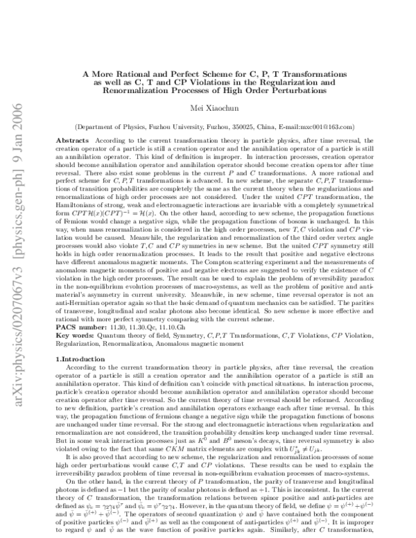
 Mei Xiaochun