Ecological Modelling 247 (2012) 273–285
Contents lists available at SciVerse ScienceDirect
Ecological Modelling
journal homepage: www.elsevier.com/locate/ecolmodel
Compartment-based hydrodynamics and water quality modeling of a Northern
Everglades Wetland, Florida, USA夽
Hongqing Wang a,∗ , Ehab A. Meselhe b , Michael G. Waldon c , Matthew C. Harwell d , Chunfang Chen e
a
U.S. Geological Survey, National Wetlands Research Center, Baton Rouge, LA 70803, USA
The Water Institute of the Gulf, One American Place, 301 Main St, Suite 2000, Baton Rouge, LA 70825, USA
110 Seville Blvd, Lafayette, LA 70503, USA
d
US EPA Gulf Ecology Division, One Sabine Island Drive, Gulf Breeze, FL 32561, USA
e
Center for Louisiana Inland Waters Studies, Institute of Coastal Ecology and Engineering, University of Louisiana at Lafayette, P.O. Box 42291, Lafayette, LA 70504, USA
b
c
a r t i c l e
i n f o
Article history:
Received 3 May 2012
Received in revised form 5 September 2012
Accepted 7 September 2012
Available online 29 September 2012
Keywords:
Everglades
Compartmental modeling
Hydrodynamics
Water quality
Water managment
Sensitivity analysis
a b s t r a c t
The last remaining large remnant of softwater wetlands in the US Florida Everglades lies within the Arthur
R. Marshall Loxahatchee National Wildlife Refuge. However, Refuge water quality today is impacted by
pumped stormwater inflows to the eutrophic and mineral-enriched 100-km canal, which circumscribes
the wetland. Optimal management is a challenge and requires scientifically based predictive tools to
assess and forecast the impacts of water management on Refuge water quality. In this research, we
developed a compartment-based numerical model of hydrodynamics and water quality for the Refuge.
Using the numerical model, we examined the dynamics in stage, water depth, discharge from hydraulic
structures along the canal, and exchange flow among canal and marsh compartments. We also investigated the transport of chloride, sulfate and total phosphorus from the canal to the marsh interior driven
by hydraulic gradients as well as biological removal of sulfate and total phosphorus. The model was
calibrated and validated using long-term stage and water quality data (1995–2007). Statistical analysis indicates that the model is capable of capturing the spatial (from canal to interior marsh) gradients
of constituents across the Refuge. Simulations demonstrate that flow from the eutrophic and mineralenriched canal impacts chloride and sulfate in the interior marsh. In contrast, total phosphorus in the
interior marsh shows low sensitivity to intrusion and dispersive transport. We conducted a rainfall-driven
scenario test in which the pumped inflow concentrations of chloride, sulfate and total phosphorus were
equal to rainfall concentrations (wet deposition). This test shows that pumped inflow is the dominant factor responsible for the substantially increased chloride and sulfate concentrations in the interior marsh.
Therefore, the present day Refuge should not be classified as solely a rainfall-driven or ombrotrophic
wetland. The model provides an effective screening tool for studying the impacts of various water management alternatives on water quality across the Refuge, and demonstrates the practicality of similarly
modeling other wetland systems. As a general rule, modeling provides one component of a multi-faceted
effort to provide technical support for ecosystem management decisions.
© 2012 Published by Elsevier B.V.
1. Introduction
Abbreviations: CA, cluster analysis; CL, chloride; DMSTA, dynamic model for
storm water treatment; EAA, everglades agricultural area; ET, evapotranspiration;
SFWMD, South Florida Water Management District; STA, stormwater treatment
area; SO4 , sulfate; SRSM, simple refuge screening model; TP, total phosphorus;
USACE, U.S. Army Corp of Engineers; USEPA, U.S. Environmental Protection Agency;
USFWS, U.S. Fish and Wildlife Service; USGS, U.S. Geological Survey; WCA, water
conservation area.
夽 Peer review disclaimer: This draft manuscript is distributed solely for purposes
of scientific peer review. Its content is deliberative and predecisional, so it must
not be disclosed or released by reviewers. Because the manuscript has not yet been
approved for publication by the U.S. Geological Survey (USGS), it does not represent
any official USGS finding or policy.
∗ Corresponding author. Tel.: +1 850 443 7870; fax: +1 225 578 7927.
E-mail address: wangh@usgs.gov (H. Wang).
0304-3800/$ – see front matter © 2012 Published by Elsevier B.V.
http://dx.doi.org/10.1016/j.ecolmodel.2012.09.007
The Arthur R. Marshall Loxahatchee National Wildlife Refuge
(Refuge), which overlays Water Conservation Area 1 (WCA1), is an
impounded freshwater marsh established in the 1950s for protection of wildlife habitat (e.g., the endangered Everglade snail kite) as
well as sources of water supply to croplands, water storage across
the dry and wet seasons, and flood protection to the neighboring
urban environment (Brandt et al., 2004; USFWS, 2007). The Refuge
is a remnant of the once contiguous Everglades that extended from
the Kissimmee Chain of Lakes south to Florida Bay. In the historic
Everglades, water generally flowed from north to south following
the natural elevation gradient as sheet flow. Presently, the Refuge
marsh is encircled by a 100-km levee and its associated borrow
�274
H. Wang et al. / Ecological Modelling 247 (2012) 273–285
canal with an average width of 40 m, which was completed by the
U.S. Army Corps of Engineers in the early 1960s.
Land use in the drainage basin upstream of the Refuge has
changed from historic Everglades marsh to primarily agriculture
and some urban use. This change has resulted in substantially elevated nutrient and mineral concentrations in the inflow into the
Refuge (USFWS, 2007). Water quality even in the interior marsh of
the Refuge has been affected by intrusion of eutrophic and mineralenriched waters in the canal that surrounds the Refuge (Gilmour
et al., 2008; Harwell et al., 2008; Surratt et al., 2008; Wang et al.,
2009; Chen et al., 2012). There are two major mechanisms responsible for the increase in nutrient and mineral concentrations in
the Refuge, inflow and intrusion. First, inflows into the Refuge
from pumped agricultural stormwater runoff (USFWS, 2007) bring
agricultural nutrients and elevated mineral concentrations to the
Refuge. Nearly half of the average annual water inputs to the Refuge
originate in these inflows, with direct rainfall accounting for the
remainder (Arceneaux et al., 2007; Meselhe et al., 2010). Constructed wetlands, termed Stormwater Treatment Areas (STAs),
bordering the northern part of the Refuge were created to remove
total phosphorus (TP), often removing over 80% of TP, but they
remove less than 20% of sulfate (SO4 ) (He, 2007). Second, rather
than being discharged from the Refuge rim canal through outflow
structures that discharge to WCA2, much of the inflow enters the
Refuge interior marsh as overbank flows from the canals, similar to
a floodplain wetland, resulting in elevated concentrations of nutrient and minerals in marsh interior (Harwell et al., 2008; Surratt
et al., 2008). Modeling presented here quantifies these mechanisms
and their impacts.
Degradation of water quality in the Refuge could greatly
affect the structure, function, and health of the Refuge ecosystem. Phosphorus enrichment is a major driving factor responsible
for vegetation and landscape changes within the Refuge and
across WCA2A (McCormick et al., 2009). Most of the ecological
responses to phosphorus enrichment ultimately occur within a relatively narrow range of water-column TP concentration between
approximately 0.01 and 0.03 mg l−1 (10 and 30 g l−1 ) (McCormick
et al., 2002). Therefore, even a small change in TP concentration may cause substantial shifts in native biological populations
(McCormick et al., 2002). Recognizing this sensitivity, the State of
Florida set the numerical criterion for TP in the Refuge at a geometric mean of 0.01 mg l−1 (10 g l−1 , Walker and Kadlec, 2011). As for
the ecological impact of SO4 , previous studies (Bates et al., 1998;
Gilmour et al., 1998, 2008; Orem et al., 2002) indicated that high
levels of SO4 entering the Everglades marsh could stimulate microbial sulfate reduction, causing buildup of sulfide in pore water,
and production of methylmercury (a neurotoxin to fish and other
wildlife).
It is a challenge for the Refuge to identify management
alternatives that maximize benefits for wildlife while meeting
constraints of flood control and water supply. The optimal management requires physical-based predictive tools to assess and
forecast the impacts of water management on Refuge water quality.
Integrated hydrodynamic and water quality models provide such
predictive capability. Previously, there have been limited modeling
efforts that link hydrodynamics and water quality in the Refuge.
The Everglades Landscape Model (ELM) (Fitz and Trimble, 2006;
Fitz et al., 2011), which imports part of its flow simulation from the
South Florida Water Management Model (SFWMM) (South Florida
Water Management District, 2005), simulates hydrology and water
quality in a large area of South Florida including the Refuge but
at a coarse resolution (2-mile × 2-mile) with consideration of discharge only for major hydraulic structures within the model grid.
The commercial MIKE-FLOOD model combined with ECOLab (DHI,
http://www.mikebydhi.com/Products/ECOLab.aspx) has also been
used to simulate Refuge stage and water quality at a high spatial
resolution (400-m × 400 m; Chen et al., 2010, 2012). While this
model performs well, it is computational costly. It requires very
long run time relative to the model presented here, and requires
a significant level of user training and sophistication. Arceneaux
et al. (2007) conducted water budget and water quality modeling for the Refuge using concentric four-compartment delineation
(one canal compartment, and three inner marsh compartments)
termed the Simple Refuge Screening Model (SRSM). Such delineation was not sufficient to capture the large spatial variations in
hydrodynamics and constituent transport among different areas
where the characteristics of soil, topography, and vegetation show
spatial heterogeneity within the Refuge (e.g., variations in water
quality parameters in marsh areas along the east and west of the
rim canal). Development of the SRSM has continued (Meselhe et al.,
2010; Roth and Meselhe, 2010), and it has been applied in a number of management applications where Refuge-wide aggregated
results are of interest. The model described herein evolved from
the concept of the SRSM, and was conceived to provide a compartmental model, which combines ease-of-use and computational
efficiency, similar to that of the SRSM, but with improved spatial
resolution. It should be noted that each of these Refuge models
has particular applications for which they are useful, and no model
meets all needs.
Identification of superior management strategies requires
answering questions such as what conditions (e.g., timing and location of structure inflows) would cause canal water intrusion into the
marsh interior, and what inflow amount and concentrations would
lead to spikes of TP and SO4 in the marsh interior? In this research,
our objectives are to: (1) develop a spatially-lumped model to
examine the spatial and temporal variations in water quantity and
water quality parameters (CL, TP and SO4 ) in the Refuge; and (2)
examine the influence of canal water on marsh water quality in
the Refuge through scenario analyses in a fast and computationally
efficient way.
2. Methods
2.1. Study site
The Arthur R. Marshall Loxahatchee National Wildlife Refuge
is located in the subtropical region of South Florida (latitude
26◦ 21.36′ to 26◦ 41.04′ N; longitude 80◦ 13.32′ to 80◦ 26.7′ W; Fig. 1).
It is bordered on the northwest by drained wetlands converted to
Fig. 1. Location of the A.R.M. Loxahatchee National Wildlife Refuge (LNWR), Florida
(inset) and distribution of hydraulic structures and water level stations in the Refuge.
�H. Wang et al. / Ecological Modelling 247 (2012) 273–285
275
agriculture known as Everglades Agricultural Area (EAA), by urban
development on the east, and on the southwest by WCA2. Much of
the average annual rainfall, approximately 1400 mm, occurs during
May to October (wet season), and more than half of this annual
rainfall occurs between June and September (USFWS, 2000). Soils
in the Refuge are classified as Histosols, and have an average thickness of 2–3 m. Refuge interior marsh soil elevations range from 3.2
to 5.6 m (1929 NGVD), and gently decline from north to south with
a slight gradient of 2–3 cm/km (USFWS, 2007; Marchant et al.,
2009). The Refuge covers 57,085 ha (141,000 acres) of marsh. The
marsh is a mosaic of habitats including slough, wet prairie, sawgrass, brush, tree islands, and cattail (USFWS, 2000). The Refuge
provides habitat for over 300 vertebrate species including the
endangered Everglade snail kite and wood stork (USFWS, 2000).
Water is released from the perimeter canal through southwestern and eastern gated structures of S-10E, S-10D, S-10C, S-10A,
S-39, G-94C, G-94A, and G-94B. Several structures, including S-5AS,
G-338, G-301, and G-300, are bidirectional. There are six continuous
water level stations established and operated by the USGS: five of
them are located in the Refuge interior (1–7, 1–9, 1–8T, Lox North,
and Lox South), and one located in the rim canal (1–8C) (Fig. 1).
2.2. Data acquisition
The hydrological, meteorological, and water quality data were
obtained mainly from the South Florida Water Management
District (SFWMD) DBHYDRO database (http://www.sfwmd.gov/
dbhydroplsql/show dbkey info.main menu). The data were collected and compiled for January 1, 1995 to December 31, 2007,
which corresponded to our study period. The concentrations of CL,
TP and SO4 at hydraulic structures were measured various frequencies including biweekly, monthly or quarterly depending on the
specific constituent and sampling periods (e.g., SO4 in most inflows
is measured quarterly).
Monitoring data for model calibration and validation are available from water quality monitoring sites. Observations within the
canal are available at outflow hydraulic structures (i.e., S-39, S10A, S-10C, S-10D, and S-10E; Fig. 1), and monitoring data within
the Refuge are available from SFWMD Everglades Protection Area
(EVPA) interior marsh sites (14 sites), SFWMD District Transect
monitoring sites (XYZ sites) (9 marsh sites and 2 canal sites), and
the Refuge’s Enhanced Monitoring sites by USFWS (34 marsh sites
and 5 canal sites; Fig. 2) (Harwell et al., 2008; Surratt et al., 2008).
We used data from 2004 to 2007 as the calibration period because
a more complete set of observations was available for this period
(e.g., monitoring at the Enhanced sites started in September 2004),
and we had greater confidence in the more recent data. We used
the period from 1995 to 2003 for model validation. A value of onehalf of the detection limit was used for sulfate concentration when
observed concentration was reported as below the limit of quantification (USFWS, 2007).
2.3. Classification of water quality zones
Wang et al. (2008) applied cluster analysis (CA) to objectively
determine the number of compartments and to spatially delineate
compartments with similar descriptive features in the Refuge for
water quality modeling. The delineation was based on the analysis of concentrations of CL, TP, SO4 , and calcium measured during
1995–2006 at sites distributed throughout the Refuge (Fig. 2). The
Refuge was classified into six marsh compartments: Perimeter East
(PE), Perimeter West (PW), Transition East (TE), Transition West
(TW), Interior North (IN), and Interior South (IS), and three canal
segments: Canal East (CE, corresponding to the L-40 Canal), Canal
Northwest (CN, corresponding to the L-7 Canal), and Canal Southwest (CS, corresponding to L-39 Canal) (Fig. 2). Interested readers
Fig. 2. Map of the nine water quality compartments defined by cluster analysis
and water quality monitoring stations in the A.R.M. Loxahatchee National Wildlife
Refuge (LNWR), Florida.
are referred to Wang et al. (2008) for more details on selection of the
four water quality parameters in the CA, inclusion of water quality
monitoring stations within each compartment, selection of cut-off
distance for determining the best number of clusters, and statistics
of the classified water quality zones in the Refuge.
2.4. Model and simulation platform
The state variables in this model include hydrodynamics variables (discharge and compartmental volume), and water quality
variables (CL, TP, and SO4 compartmental mass). Stage and depth
are calculated from volume. Consistent with our source data, TP
mass is measured as phosphorus, not phosphate, and SO4 mass
is measured as sulfate, not sulfur. We selected a link-node model
design (Fig. 3) because link-node models are conceptually straightforward, and computationally efficient. This compartment-based
model allows us to simulate stage and constituents (CL, TP, and SO4 )
in the rim canal and marsh areas for multiple years in a few minutes
on a desktop computer. Input data include daily inflows, outflows
(including water supply and hurricane releases), precipitation, ET,
and inflow concentrations of CL, TP, and SO4 . All three constituents
are simulated based on mass balance. For canal compartments, the
constituent transport includes loads through hydraulic structure,
flow (advective), dispersion, aerial deposition, groundwater and
biological reactive processes. For marsh compartments, mass was
calculated from all these sources except hydraulic structure load.
The dispersive mass flux is calculated by:
A
M = kd �C
L
(1)
�276
H. Wang et al. / Ecological Modelling 247 (2012) 273–285
Fig. 3. Diagram of link-node structure of the Simple Refuge Model (SRM). SRM
includes six marsh compartments (PE = perimeter east, PW = perimeter west,
TE = transition east, TW = transition west, IN = interior north, and IS = interior south)
and three canal segments (CE = canal east, CN = canal northwest, and CS = canal
southwest).
where Kd is the dispersion coefficient (m2 day−1 ), A is exchange
area (m2 ), L is length of a link calculated from centroid distance
(m), �C is the concentration difference between the two compartments (nodes). The CL concentration was modeled as a conservative
constituent (Harwell et al., 2008; Surratt et al., 2008; Waldon
et al., 2009; Meselhe et al., 2010), that is, no kinetic processes or
parameters were associated with CL modeling. The reactive loss
of SO4 resulting from microbial sulfate reduction in the underlying sediments of the marsh was estimated from the apparent
settling coefficients incorporated in the model. The reactive loss
of TP was estimated based on a biologically stored TP component that regulates P uptake, recycling, and generation of stable TP
stored in accreting peat (a permanent storage component) using
the Dynamic Model for Storm Water Treatment (DMSTA2) model
(http://wwwalker.net/dmsta/doc/doc pcycle.htm) (Walker, 1995;
Walker and Kadlec, 2005, 2011). Total phosphorus was modeled
under two vegetation conditions: emergent macrophyte vegetation (EMG, peat) and preexisting wetland (PEW, wetland vegetation
existed naturally). The detailed description of other model equations for hydrodynamic and mass transport of CL, TP and SO4 are
given in Appendix A. Values of model parameters and constants
are from literature or calibration of this study. They are summarized in Table 1 and also described in Waldon et al. (2009). Internal
TP loading (remobilization of TP from sediments to water column)
in canal compartments was calibrated to 0 mg m−2 yr−1 . That is, TP
is modeled as a conservative within the canal.
The hydrodynamics and water quality integrated model is
implemented using the differential equations solver, Berkeley Madonna (version 8.3.9) (http://www.berkeleymadonna.com),
which is a proprietary software developed by Macey et al. (2000).
Numerical method was fourth order Runge–Kutta (RK4) with a time
step of 0.005 day (7.2 min), and output was stored daily. Details
about application of Berkeley Madonna for Refuge modeling can be
found in Meselhe et al. (2009).
2.5. Impact of rim canal water intrusion on marsh water quality
In order to analyze the impact of canal water intrusion on spatial and temporal variations in water quality in the Refuge marsh,
we defined a canal water intrusion event when two conditions
were met: (1) net inflow larger than 32 m3 s−1 ; and (2) the stage
difference between canal and marsh exceeded than 0.07 m. These
conditions were based on a previous study using conductivity data
along transects in the Refuge (Surratt et al., 2008). Surratt et al.
(2008) found that it might take a few days (e.g., 4–7 days) for canal
water to intrude into the interior marsh during an intrusion event.
Therefore, we compared the simulated water quality during the
intrusion events with a 7-day window for each event with water
quality averaged over the 13 years to examine the impact of canal
water intrusion. Approximately 4% of the study period (1995–2007)
or 162 days were identified as intrusion days. The longest continuous intrusion event lasted for 12 days from August 4 to August
15, 2003. Historically, prior to its establishment in 1951, the Refuge
Table 1
Parameters and constants used in the Refuge hydrodynamics and water quality modeling (1995–2007).
Parameter
Description
Unit
Value
Source
Physical
lseep
rseep
B1
B2
B5
fETmin
Het
evap
kd
Canal seepage constant
Marsh seepage constant
Transport coefficient between canal and marsh compartments
Transport coefficient between marsh and marsh compartments
Transport coefficient between canal and canal segments
Minimum ET reduction factor
Depth below which ET is reduced
Fraction of ET that is evaporation
Dispersion coefficient
day−1
day−1
m−1 day−1
m−1 day−1
m−1 day−1
m2 day−1
0.042
0.000131527
3
14
450
0.2
0.25
0.65
43,200
Arceneaux et al. (2007)
Arceneaux et al. (2007)
This study
This study
This study
Arceneaux et al. (2007)
Arceneaux et al. (2007)
Arceneaux et al. (2007)
This study
Biological
KmaxSO4 (D)
k
KhalfSO4 (D/k)
K1tp
K2tp
K3tp
InterP
Sulfate maximum removal rate
Sulfate settling coefficient
Sulfate half saturation constant
Total phosphorus maximum uptake rate
Total phosphorus recycle rate
Total phosphorus burial rate
Total phosphorus internal loading rate
g m−2 yr−1
m yr−1
g m−3
m3 g−1 yr−1
m2 g−1 yr−1
yr−1
mg m−2 yr−1
14.4
14.4
1
0.1064 (EMG) 0.2210 (PEW)
0.0020 (EMG) 0.0042 (PEW)
0.3192 (EMG) 0.6631 (PEW)
0
Wang et al. (2009)
Wang et al. (2009)
Wang et al. (2009)
Walker and Kadlec (2005)
Walker and Kadlec (2005)
Walker and Kadlec (2005)
This study
Constants
wd cl
dd cl
wd tp
dd tp
wd so4
dd so4
Wet deposition, chloride
Dry deposition, chloride
Wet deposition, total phosphorus
Dry deposition, total phosphorus
Wet deposition, sulfate
Dry deposition, sulfate
mg l−1
mg m−2 yr−1
mg l−1
mg m−2 yr−1
mg l−1
mg m−2 yr−1
2
1136
0.01
40
1
138.2
Walker (1995)
Walker (1995)
Walker (1995)
Walker (1995)
Gilmour et al. (2008), He (2007)
Wang et al. (2009)
m
�H. Wang et al. / Ecological Modelling 247 (2012) 273–285
277
Table 2
Model performance statistics for stage, chloride, sulfate and total phosphorus for canal and marsh components in the Refuge during 1995–2007.
Statistic
CN
Stage (m, NGVD29)
−0.003
Bias
4.910
Ave. Obs.
Ave. Sim.
4.907
VR
0.78
R
0.88
Efficiency
0.78
−1
Chloride (mg l )
Bias
−20.12
128.31
Ave. Obs.
Ave. Sim.
108.19
0.47
VR
0.69
R
0.16
Efficiency
−1
Sulfate (mg l )
Bias
−13.13
55.26
Ave. Obs.
42.13
Ave. Sim.
0.60
VR
R
0.78
Efficiency
0.27
Total phosphorus (mg l−1 ) PEW
0.003
Bias
0.039
Ave. Obs.
0.042
Ave. Sim.
0.58
VR
R
0.77
Efficiency
0.57
Total phosphorus (mg l−1 ) (EMG)
Bias
0.005
Ave. Obs.
0.039
Ave. Sim.
0.045
VR
0.59
R
0.77
Efficiency
0.56
CS
CE
0.052
4.910
4.962
0.73
0.86
0.68
0.001
4.962
4.963
0.76
0.87
0.76
PW
0.055
4.915
4.970
0.72
0.85
0.68
TW
PE
0.058
4.915
4.973
0.72
0.85
0.67
TE
0.047
4.947
4.994
0.75
0.87
0.70
IN
0.049
4.947
4.996
0.74
0.86
0.69
−0.052
5.005
4.954
0.66
0.87
0.45
IS
−0.062
4.996
4.934
0.78
0.90
0.69
−8.74
107.69
98.95
0.53
0.75
0.45
10.82
80.37
91.19
−0.10
0.37
−0.23
−41.85
119.81
77.96
0.33
0.60
−1.32
−20.27
81.09
60.83
0.52
0.72
0.15
−7.06
61.47
54.40
−0.21
0.49
−0.32
−10.51
61.64
51.14
0.16
0.47
0.03
−16.17
46.76
30.58
0.39
0.63
0.07
7.55
24.24
31.79
−2.24
−0.08
−2.80
−12.95
51.94
38.98
0.46
0.68
0.14
−0.03
29.96
29.93
0.05
0.40
0.05
−21.44
47.47
26.03
0.44
0.67
−0.59
−6.42
24.32
17.90
0.48
0.69
0.34
3.48
10.98
14.46
0.19
0.45
0.13
0.77
12.79
13.56
0.08
0.37
0.08
−2.48
6.70
4.21
0.39
0.63
0.30
0.68
2.34
3.02
−0.44
0.00
−0.46
0.003
0.046
0.049
0.09
0.68
0.08
−0.035
0.086
0.051
0.14
0.38
−0.01
−0.006
0.021
0.015
−0.01
0.21
−0.13
−0.004
0.009
0.007
−0.19
0.05
−0.32
−0.044
0.055
0.011
0.07
0.48
−0.44
−0.007
0.013
0.006
−0.03
0.11
−0.45
−0.002
0.008
0.006
−0.05
0.24
−0.29
−0.005
0.009
0.004
−0.04
0.10
−1.59
0.006
0.046
0.051
0.11
0.68
0.07
−0.031
0.086
0.055
0.15
0.38
0.02
−0.001
0.021
0.020
−0.03
0.25
−0.04
0.001
0.009
0.010
−0.44
0.04
−0.46
−0.039
0.055
0.016
0.08
0.42
−0.32
−0.022
0.013
0.010
−0.23
0.02
−0.30
−0.001
0.008
0.007
−0.12
0.21
−0.15
−0.004
0.009
0.005
−0.11
0.02
−1.07
Note: Ave. Obs. = average of observed values, Ave. Sim. = average of simulated values, VR = variance reduction, R = correlation coefficient, Efficiency = Nash–Sutcliffe efficiency,
CN = canal northwest, CS = canal southwest, CE = canal east, PW = perimeter west, TW = transition west, PE = perimeter east, TE = transition east, IN = interior north, IS = interior
south. Total phosphorus was modeled under two vegetation conditions: emergent marsh (EMG) and preexisting wetland (PEW).
was an oligotrophic peatland system that received most of its water
and nutrients from rainfall (Davis, 1994). Therefore, we modeled
a completely rainfall-driven scenario for CL, TP and SO4 in which
rim canal inflow concentrations of CL, TP and SO4 were set equal
rainfall concentrations and used to model wet atmospheric deposition (Table 2). Comparison of this scenario with our base model
run allows us to quantify the impacts of elevated concentrations of
pumped inflow on marsh water quality, as well as specific intrusion
and non-intrusion events.
2.6. Statistical analysis
We used a number of common statistical measures to evaluate model performance during both calibration and validation
and entire study period (1995–2007). These measures include
bias, correlation coefficient (R), variance reduction (VR), and
Nash–Sutcliffe efficiency (Efficiency) (Nash and Sutcliffe, 1970;
Legates and McCabe, 1999). Appendix B details these calculations
and implications of these statistical measures. Some reduction
of model performance during the validation period (1995–2003)
compared with model performance during the calibration period
(2004–2007) is expected, but any large reduction would suggest
that the model fit may not be robust, or that some important factor
changed between the periods and is no longer simulated properly.
2.7. Sensitivity analysis
We conducted a formal sensitivity analysis of model outputs to
parameters over the calibration period (2004–2007). There are a
total of 15 model parameters (excluding the sulfate half saturation
constant or KhalfSO4 that is the ratio of sulfate maximum removal
rate (D) to sulfate settling coefficient (k) in Table 1) in the model
that can be divided into two types: physical and biological factors.
Physical factors are the parameters that control the physical processes (e.g., inflows, seepage, ET, dispersion, etc.) while biological
factors are those that determine the biological processes in water
quality constituents (e.g., vegetation TP uptake, burial and sulfate
reduction). Some of the physical parameters have been estimated
in previous studies (Arceneaux et al., 2007; Meselhe et al., 2010)
and the best estimates were used in this research. The best estimates of the transport coefficients, dispersion coefficient and all
biological parameters were obtained by a calibration process in
which the closest agreement between simulation and observation
on stage and water quality variables was reached. Sensitivity analysis of the parameters was performed prior to further calibration in
order to simplify the calibration procedure. In the sensitivity analysis, parameters were changed by ±25% (varying one parameter at
a time) followed the protocol of Fitz and Trimble (2006) to observe
the corresponding changes in stage and water quality variables. The
relative sensitivity index (RSI) of parameter i to state variable j was
defined using the following equation:
RSI(Pi , Xj ) =
�
�Xj /Xj
�Pi /Pi
�
× 1000
(2)
where Pi is parameter i, Xj is state variable j (or stage, concentrations of CL, TP and SO4 ), �Pi is the change in parameter i, � Xj is
the change in average value of state variable j over the period of
2004–2007 due to the parameter change. The higher the RSI of a
�278
H. Wang et al. / Ecological Modelling 247 (2012) 273–285
parameter, the more sensitive the model is to that parameter. An
RSI value of 1000 means that the relative change in a variable equals
that of the parameter of interest. Negative values of RSI indicate
the negative relationship between parameter change and change
in state variable. A mean RSI of parameter i to all variables (stage,
concentrations of CL, TP and SO4 in both canal and marsh) was generated from the absolute values of individual RSIs to indicate the
overall importance of a parameter in the model.
3. Results
3.1. Model performance
3.1.1. Stage and outflow
Because the magnitudes and seasonal patterns in both simulated
and observed stage at all the compartments are similar, or insensitive to spatial pattern, we selected Canal Southwest and Transition
West as two examples to illustrate comparisons between simulated
and observed daily stage at canal and marsh in the Refuge (Fig. 4).
Daily water level data at S-10D and the average daily water level
data of S-10D and G-301 were used as observed stage for Canal
Southwest and Transition West, respectively. Statistics for all nine
compartments are given in Table 2. Daily water level data at G301 and 1–8C along the canal were used for comparisons for Canal
Northwest and Canal East. For other marsh compartments, daily
water level data at 1–8T, Lox North and Lox South were used in
the comparisons. Our hydrodynamics model generally reproduced
the observed daily water levels and captured the overall trends and
seasonal variations in stage for the canal and marsh compartments
(Table 2 and Fig. 4). Over the entire simulation period (1995–2007),
simulated stage showed good agreement with observations for
both the canal and marsh compartments with low bias, high variance reduction, high correlation coefficient and high Nash–Sutcliffe
efficiency. Model biases were smaller for the canal (0.001–0.052 m)
than for the marsh (0.047–0.062 m), for the marsh near the east
canal (0.047–0.049 m) than for the marsh near the west canal
(0.055–0.058), and for the interior north (0.052 m) than for the
interior south (0.062 m). Correlation coefficients were >0.85 for
Fig. 4. Comparison between simulated and observed daily stage in selected canal
(top panel) and marsh components (bottom panel) in the Refuge during 1995–2007.
all compartments. Values of variance reduction and Nash–Sutcliffe
efficiency were larger than 0.7 and 0.67 for all compartments except
Interior North (0.66 and 0.45, respectively). The consistency among
correlation coefficient, variance reduction and Nash–Sutcliffe efficiency for canal and marsh (except Interior North) indicates that the
model produced similar magnitudes, trends and temporal patterns
in water level compared to the observations.
This model also simulated monthly outflow very well. The values of variance reduction, correlation coefficient and Nash–Sutcliffe
efficiency were 0.74, 0.87 and 0.74, respectively. This addition to
the model is very important in terms of predicting impacts of water
management alternatives and regulation schedule on Refuge water
quality.
3.1.2. Water quality parameters
Plots comparing simulated and observed water quality concentrations (CL, SO4 and TP) are given in Figs. 5–7. Canal Southwest was
used as an example for model performance assessment for canal
compartments while Transition West and Interior North were used
as examples for marsh compartments. Monthly averaged values of
both simulation and observation were used in the comparisons.
These three compartments were selected for model performance
assessment because at least six sites from EVPA, XYZ and enhanced
monitoring sites with field data could be used to represent the
water quality conditions within these compartments. For example, there were 27 monitoring sites within Interior North. Some
compartments such as Perimeter West, Perimeter East and Canal
Northwest had three sites or less and may not be sufficient in representing the water quality condition in the compartments in which
they are located for reliable comparisons. Statistics of model performance for all nine compartments are provided in Table 2.
Overall, the observed data and the water quality simulation
results show close agreements in spatial and temporal (inter-
Fig. 5. Comparison between simulated and observed monthly averaged concentrations of chloride (CL) in selected canal (top panel) and marsh compartments (middle
and bottom panels) in the Refuge during 1995–2007.
�H. Wang et al. / Ecological Modelling 247 (2012) 273–285
Fig. 6. Comparison between simulated and observed monthly averaged concentrations of sulfate (SO4 ) in selected canal (top panel) and marsh compartments (middle
and bottom panels) in the Refuge during 1995–2007.
annual and seasonal) variation in the concentrations of CL, SO4 and
TP for most compartments. The model tended to underestimate
concentrations of CL and SO4 for both marsh and canal zones and TP
concentration for marsh areas (Table 2; Figs. 5–7). Model simulations captured three water quality gradients that are also shown by
field observations: (1) west gradient: west canal ≥ perimeter west
marsh ≥ transition west marsh ≥ interior marsh; (2) east gradient:
east canal ≥ perimeter east marsh ≥ transition east marsh ≥ interior
marsh; and (3) north-south gradient (Table 2). The model simulated the three water quality concentrations better for canal
compartments than for marsh compartments. For those compartments with low or negative variance reductions and Nash–Sutcliffe
efficiencies, the model is less successful at explaining the temporal
patterns of CL, SO4 and TP. The water quality model tended to
simulate CL concentration better than SO4 and TP concentrations.
Compared to the performance in stage simulations, the model is
clearly less successful in simulating concentrations of CL, SO4 and
TP. This is not surprising since any water quality model can only
be as good as the hydrodynamic model that drives the transport of
water constituents in the system.
3.2. Sensitivity analysis
Overall, the model is most sensitive to three parameters, fraction of ET that is evaporation (evap), water depth below which
ET is reduced (Het ), and dispersion coefficient (kd ) (Table 3). Values for these three parameters have greater impact on the model
performance than the others. Moreover, for different state variables and Refuge zones, the three most important parameters of
impact could be different. For example, for stage in the canal and
the marsh, water depth below which ET is reduced (Het ) is the most
important parameter followed by the canal seepage constant (lseep)
279
Fig. 7. Comparison between simulated and observed monthly averaged concentrations of total phosphorus (TP) in selected canal (top panel) and marsh compartments
(middle and bottom panels) in the Refuge during 1995–2007. Two different simulations are presented: PEW = pre-existing wetland condition; EMG = emergent marsh
condition.
and the marsh seepage constant (rseep). For CL in the canal and
the marsh compartments, fraction of ET that is evaporation (evap),
water depth below which ET is reduced (Het ) and dispersion coefficient (kd ) are the three most important parameters (Table 3). In
terms of TP in the marsh compartments, the model is sensitive to
the maximum uptake rate of total phosphorus (k1tp, RSI = -547.4),
recycle rate of total phosphorus (k2tp, RSI = 448.6) and water depth
below which ET is reduced (Het , RSI = -267). For TP in the canal
compartments, internal P loading rate (interP, RSI = 217.5), dispersion coefficient (kd, RSI = −194.8) and water depth below which ET
is reduced (Het , RSI = −172.2) are the three parameters to which
the model is most sensitive. For SO4 in the marsh, the model
is most sensitive to sulfate maximum removal rate (KmaxSO4,
RSI = −384.1), fraction of ET that is evaporation (evap, RSI = 288.9)
and dispersion coefficient (kd, RSI = 227.1). For SO4 in the canal,
dispersion coefficient (kd, RSI = −116.7), water depth below which
ET is reduced (Het , RSI = −106.2) and sulfate maximum removal
rate (KmaxSO4, RSI = −87.9) are the three most important parameters (Table 3). To a larger degree, sensitivity analysis indicates
that evapotranspiration-related factors determine the model performance for both hydrodynamics and water quality. It appears that
hydrological processes control the status of all the three water quality variables in the canal and also chloride in the marsh whereas
biological processes, together with physical processes, control the
dynamics of TP and SO4 in the marsh.
3.3. Impact of canal water on marsh water quality
Our numerical modeling provides quantitative evidence that
water quality in the perimeter and transitional zones and even
the marsh interior is affected by the intrusion of rim canal water
�280
H. Wang et al. / Ecological Modelling 247 (2012) 273–285
Table 3
Relative sensitivity index (RSI) of parameters in the Refuge hydrodynamic and water quality model.
Parameter
Zone
Stage
CL
TP
SO4
lseep
Canal
Marsh
Canal
Marsh
Canal
Marsh
Canal
Marsh
Canal
Marsh
Canal
Marsh
Canal
Marsh
Canal
Marsh
Canal
Marsh
Canal
Marsh
Canal
Marsh
Canal
Marsh
Canal
Marsh
Canal
Marsh
Canal
Marsh
−14.6
−6.1
−5.7
−2.9
3.5
0.3
6.4
0.9
−0.6
0.1
−0.2
−0.3
27.7
13.9
0.0
0.0
0.0
0.0
0.0
0.0
0.0
0.0
0.0
0.0
0.0
0.0
0.0
0.0
0.0
0.0
−39.7
−90.3
4.5
−11.9
1.9
10.3
−1.5
−0.6
−9.1
1.0
1.4
2.3
−88.8
−132.2
218.2
665.0
−62.9
105.3
0.0
0.0
0.0
0.0
0.0
0.0
0.0
0.0
0.0
0.0
0.0
0.0
27.6
71.9
33.2
47.6
−3.4
10.1
−35.0
−13.9
−30.5
2.4
2.5
5.9
−172.2
−267.0
6.0
56.1
−194.8
55.7
0.0
0.0
0.0
0.0
−125.1
−547.4
105.0
448.6
−56.5
−68.0
217.5
53.8
−22.0
−109.8
18.1
12.1
4.6
45.0
−9.8
32.8
−13.0
5.9
1.4
3.4
−106.2
−150.1
69.3
288.9
−116.7
227.1
12.9
90.4
−87.9
−384.1
0.0
0.0
0.0
0.0
0.0
0.0
0.0
0.0
rseep
B1
B2
B5
fETmin
Het
evap
kd
KhalfSO4
KmaxSO4
K1tp
K2tp
K3tp
interP
All variable
47.8
17.0
9.9
12.6
7.8
2.2
119.8
162.9
95.3
12.9
59.0
84.1
69.2
15.6
33.9
Note: Refer to Table 1 for parameter description. “All variable” column gives the mean RSI of parameter i in the context of all four state variables (stage, CL, TP, and SO4 )
combined (canal + marsh compartments). Mean RSI is an indicator of importance of each parameter in the model.
with elevated constituent concentration. If the concentrations of
CL, TP, and SO4 discharging through the inflow structures were
equal to that of wet atmospheric deposition (a rainfall-driven
condition), there would be no high concentration occurrences
above rainfall-driven marsh concentrations of CL (∼5–6 mg l−1 ),
TP (0.004–0.007 mg l−1 ), and SO4 (0.1–0.6 mg l−1 ). Elevated marsh
concentrations would also be avoided if canal water intrusion
events were eliminated. However, intrusion events would bring
canal water into the marsh interior, resulting in elevated concentrations of CL and SO4 in the marsh interior. For example, CL
concentrations would be ∼88–103 mg l−1 in the perimeter zone,
∼64–79 mg l−1 in the transitional zone, and ∼30 mg l−1 in the interior marsh (Table 4). These results represent increases of >22-fold,
>13-fold, >5-fold of the CL concentrations compared to that under
the rainfall-driven condition at the perimeter, transitional and interior marsh, respectively. For SO4 , the concentrations would be
∼32–42 mg l−1 in the perimeter zone, ∼20–29 mg l−1 in the transitional zone, and ∼4–7 mg l−1 in the interior marsh (Table 4).
Compared to the assumed rainfall-driven condition, canal water
intrusion would result in increases of >42-fold, >35-fold, and >21fold of SO4 concentrations at the perimeter, transitional and interior
marsh zones, respectively (Table 4). Moreover, even without intrusion events as defined in this research, the rim canal water with
elevated concentrations of CL and SO4 would also cause substantial increases in the concentrations at the perimeter and transitional
zones by exchange of flows and transport between canal and marsh
(8–13 and 21–56 times for CL and SO4 , respectively) and moderate
increases at the interior marsh (∼6, and 20–30 times for CL, and
SO4 , respectively) (Table 4).
For TP, the impact of canal water intrusion would be limited
within the perimeter and transition zones. TP concentrations would
be ∼0.026–0.036 mg l−1 in perimeter zone and ∼0.01–0.016 mg l−1
in transitional zone, respectively (Table 4). Compared to
the assumed reference condition (inflow equals to rainfall
concentration, 0.01 mg l−1 ), canal water would cause approximately 4.3-fold and 2.5-fold of increases in the TP concentrations
at perimeter and transition marsh, respectively. Average surface
water TP concentrations in the interior marsh, as averaged at the
coarse spatial scale shown in Fig. 3, seem not likely to be impacted
by canal water intrusion as indicated by relatively stable concentrations of 0.004–0.007 mg l−1 (Table 4).
4. Discussion
4.1. Model performance
Although the model simulates stage well, the performance
declines during dry periods (low water levels) (Fig. 4). For example, the model did not capture water level during the dry period in
Spring of 2001 (Fig. 4). This could be due to the lack of a groundwater component to account for the interaction between surface
water and groundwater in the Refuge, which was identified as an
important factor determining water budget during the Everglades
dry season (e.g., Harvey et al., 2004). Spatially, we anticipated that it
would be more difficult to accurately model the temporal variations
of water level for the marsh than for the rim canal because interior
marsh areas tend to have complicated topography and vegetation
patterns, which makes it difficult to accurately estimate ET in different marsh zones. As indicated by the sensitivity analysis (Section
3.2), the fraction of ET that is evaporation (evap) and water depth
below which ET is reduced (Het ) are the most important parameters
affecting model performance for the marsh. There is only one Het
parameter for all six marsh compartments, and the ET observations
for the marsh come from only one ET station near the Northwest
corner of the Refuge (USFWS, 2007), thus the spatial variation in
ET in the Refuge could not be fully represented in the model. It is
known that ET and the depth below which ET is reduced could be
affected by vegetation types (Abtew, 1996). Therefore, the model
�Note: PW = perimeter west, TW = transition west, PE = perimeter east, TE = transition east, IN = interior north, IS = interior south, PEW = pre-existing wetland condition, EMG = emergent marsh condition.
5.05
19.19
1.01
1.05
5.62
21.13
1.11
1.17
5.95
29.26
1.00
1.05
6.89
29.72
1.09
1.16
8.24
21.89
1.41
1.88
13.85
35.64
2.09
2.53
10.75
26.12
3.18
3.81
22.72
42.79
4.34
5.09
10.61
46.84
1.52
1.90
Ratio (actual inflow concentration/rainfall concentration)
CL
30.43
13.42
19.48
56.64
39.90
56.09
SO4
TPPEW
4.48
3.02
2.37
4.99
3.28
2.75
TPEMG
6.37
0.14
0.004
0.005
5.34
0.20
0.004
0.005
5.08
0.13
0.006
0.007
4.36
0.21
0.006
0.006
6.15
0.48
0.004
0.005
4.62
0.57
0.005
0.006
5.83
0.62
0.005
0.006
3.88
0.74
0.006
0.007
4.05
0.51
0.005
0.006
With inflow concentration as rainfall
CL
3.40
5.30
0.74
0.56
SO4
TP PEW
0.006
0.004
TPEMG
0.007
0.005
5.45
0.33
0.004
0.005
32.19
2.76
0.004
0.005
30.04
4.32
0.004
0.006
30.19
3.91
0.006
0.007
30.01
6.39
0.006
0.007
50.66
10.61
0.006
0.010
64.03
20.29
0.010
0.015
62.66
16.17
0.015
0.022
88.14
31.59
0.026
0.035
57.85
15.66
0.006
0.010
78.89
28.59
0.011
0.016
With actual inflow concentration
CL
103.44
71.07
SO4
41.83
22.46
TP PEW
0.029
0.013
0.018
0.036
TP EMG
Non-intrusion
Intrusion
period
IS
Non-intrusion
Intrusion
period
IN
Non-intrusion
Intrusion
period
TE
Non-intrusion
Intrusion
period
PE
Intrusion
period
Non-intrusion
TW
Intrusion
period
Non-intrusion
PW
Compartment
Table 4
Comparison between simulated water quality parameter (unit: mg l−1 ) with pumped inflow concentration and that with inflow concentrations equals to rainfall concentration under intrusion and non-intrusion conditions over
the period of 1995–2007 in Refuge marsh compartments.
H. Wang et al. / Ecological Modelling 247 (2012) 273–285
281
would be improved if ET measurements were available from field
stations well-distributed within the marsh.
Statistical analysis indicated that the water quality model was
unable to describe the dynamics of CL, SO4 and TP for some marsh
compartments as indicated by the low or negative variance reduction and Nash–Sutcliffe efficiency (Table 2). The model did not
capture the observed CL concentration spikes (>100 mg l−1 ) during the Spring of 2001 although it produced the highest simulated
CL concentrations (Fig. 5). This is may have resulted from the overestimated stage and volume during this dry period. The model was
not able to capture the spikes of SO4 concentration from June 1999
to July 2001 and from September 2002 to June 2003 (Fig. 6). These
SO4 spikes could not be solely explained by canal water intrusion
and dispersive transport (e.g., Wang et al., 2009), and this suggests some factor outside our model design (e.g., increased aerial
deposition or reflux from soil) may have occurred during these
periods. Local variations in topography and patterns of vegetative
resistance to flow affect canal water intrusion into different parts
of the Refuge (Surratt et al., 2008; McCormick et al., 2011), and
a better understanding of these factors might provide a basis for
model improvement. The sensitivity analysis identifies the dispersion coefficient as one of the top three parameters determining
model projections for CL and SO4 but not TP. Moreover, CL and
SO4 are more sensitive to the dispersion coefficient in the marsh
than in the canal. This suggests that dispersive transport plays an
important role in mass transport from the rim canal to the interior marsh for CL and SO4 . Our results are consistent with Chen
et al. (2012) who found that CL is transported mainly by dispersion in interior marsh while CL transport in the canal is dominated
by advection. Chen et al. (2012) found that increasing the dispersion coefficient (0.001–2.0 m2 s−1 ) from the fringe marsh to
the most interior marsh improved model performance in Refuge
water quality simulations using a 400 m regular square grid spatially explicit model. We used a constant dispersion coefficient
(kd = 43,200 m2 day−1 , or 0.5 m2 s−1 ) in our model. Our spatially
uniform dispersion coefficient, although falling within the range,
may not be able to capture the variations in the mass transport of CL
and SO4 in the interior marsh compartments. The limited number
of water quality monitoring sites within some compartments of our
model also may contribute to discrepancies with observations and
this limitation is independent of model spatial structure. The sites
in a compartment may not be representative of the water quality
conditions in the entire compartment even though that is the intention of the compartment-based model design. There was only one
water quality observation from a single monitoring station for some
periods. This single-measurement issue may cause larger discrepancies particularly when the sampled station is not representative
of the whole compartment. Moreover, missing data due to sampling
gaps at the marsh sites when water depth was too low to sample
(no samples are collected when depth of clear water is less than
10 cm) also reduced the reliability of the comparisons. Therefore,
increased sampling sites and sampling frequency might improve
the model’s statistical performance. Water quality measurement
accuracy and precision may be an additional factor limiting statistical model performance. For example, for unknown reasons marsh
TP data in portions of 1996–1997 appear to be unreasonably low
and in error (Dr. Bill Walker, pers. comm.).
4.2. Impact of canal water intrusion on marsh water quality
Both observation and model simulation suggested that
the magnitude of the gradients declines in the order of
west > east > north–south. Therefore, canal water intrusion and dispersive transport of CL and SO4 , especially from the western canal,
is the most important factor controlling Refuge marsh water quality and habitat suitability for fish and wildlife (Harwell et al., 2008;
�282
H. Wang et al. / Ecological Modelling 247 (2012) 273–285
Surratt et al., 2008). The north–south gradients of modeled CL and
SO4 generally correspond to relatively dry periods (Figs. 5 and 6)
because of the lower water depth in the North (resulting from a
topographic gradient from north to south). There tended to be no
north–south gradient for TP (Table 2), implying the importance
of vegetation and soil processes in impacting surface water TP
(e.g., plant uptake and sediment TP sequestration) (e.g., Walker and
Kadlec, 2005; Gu, 2008).
Previous studies indicated that water quality in the interior
marsh zones have been affected by canal water intrusion (e.g.,
McCormick et al., 2002, 2011; Reddy et al., 2008; Surratt et al.,
2008). For example, Reddy et al. (2008) found that the TP enrichment front extended 1.5, 2.5 and 2.0 km (or Interior North in this
study) from STA-1E, 1W and S-6 transects. Other studies identified
a phosphorus enrichment zone from the canal community pattern
extending ∼1.3–2.5 km into the interior marsh and a zone of canal
influence extending ∼4.5 km into the interior marsh in terms of
specific conductance (McCormick et al., 2002; Harwell et al., 2008).
Our simulation results (Table 4) also indicate that intrusion of canal
water tends to be greatest across the western side of the Refuge due
to the greater inflow and lower soil elevation along the southwestern perimeter that is consistent with previous studies (e.g., Surratt
et al., 2008; Marchant et al., 2009; McCormick, 2010; McCormick
et al., 2011). The position of the intrusion front was found to be
correlated with the edge of the cattail incursion in the perimeter marsh zones (e.g., Marchant et al., 2009). Our rainfall-driven
scenario test indicates that canal water intrusion impacts all of
the marsh compartments, but does not measurably affect surface
water TP in the most interior marsh (IN and IS). This is presumably because P is taken up rapidly in the perimeter and transition
zones (e.g., Walker and Kadlec, 2011), and is controlled in the interior by uptake into biological storage. Our interior marsh grid is
spatially different from the analytical designs cited above. Thus,
a larger body of information is needed to draw inferences about
water quality impacts.
Analysis of the rainfall-driven scenario shows that the rim canal
water with elevated concentrations of CL would transport significant amount of CL into the interior marsh, resulting in >5-fold
increase in CL concentrations (Table 4). One may argue that such
dramatic increases in CL concentration in the interior marsh might
be due to the concentrating effect of evaporation during the dry
season rather than exogenous pumped inflow. Our simulations
revealed that when the inflow CL concentration equals that of the
rainfall (2 mg l−1 ), the maximum CL concentration in the interior
marsh would be 23.7 mg l−1 during the dry season when ET and
seepage exceed precipitation. CL concentrations would maintain at
3–4.5 and 5–7.3 mg l−1 for the wet and dry seasons, respectively. In
contrast, with the CL concentration from the pumped inflow along
the rim canal, CL concentrations in the interior marsh would be
as high as 98.5 mg l−1 . The mean CL concentration would increase
from 27.8 mg l−1 in the wet season to 36.3 mg l−1 in the dry season. Observed average CL concentrations in the interior marsh were
∼25–46 mg l−1 (Table 2), and also showed a factor of 5–10 higher
CL concentration than it would be if driven by evaporation. Our
results are consistent with the conclusion of Chen et al. (2012) that
although evaporation during the dry season does at times increase
simulated CL concentrations, most of the chloride mass observed
at the interior marsh originates at pumped inflow rather than from
aerial deposition. Therefore, we conclude that CL concentration,
even in the interior, is currently dominated by pumped inflow. Calcium monitoring data were used to establish the spatial design of
the marsh cells (Wang et al., 2008). In future, efforts might extend
this model to include the utility of this model to understanding
calcium concentrations in the Refuge.
Simulated events of short-duration elevated SO4 concentration
(spikes) at the interior marsh (Fig. 6) indicate that canal water
penetrates and impacts the interior. Similar short-duration events
of high water column TP simulated at all marsh compartments are
eliminated when inflow is set at 0.01 mg l−1 (10 ppb).
Spatial aggregation of the model design make it inappropriate
for most site-specific applications because it is not capable of precisely simulating the pollutant intrusion fronts observed in transect
monitoring (e.g., Smith and McCormick, 2001; Reddy et al., 2008;
Surratt et al., 2008).
5. Conclusions
In this research, we developed a compartment-based water and
constituent model for the Arthur R. Marshall Loxahatchee National
Wildlife Refuge. Our goal was to balance the need to include enough
complexity to reasonably characterize the 57,085 ha wetland but
not resorting solely to using a high spatial resolution model.
Through calibration and validation using long-term (1995–2007)
field observations, our compartmental modeling approach proves
to be a conceptually straightforward and computationally efficient
screening tool for examining and predicting wetland surface water
quality distribution along the gradient from the canal to the marsh
interior. This model is useful for predicting water quality under different water management scenarios for purposes of general analyses and interpretation, including comparisons across different scenarios. No single model for water quality is suitable for all applications, this model is part of a larger suite of models designed to help
guide the management decision making processes. Our experience
suggests that similar compartmental modeling could be of value
in developing understanding and testing alternatives for management for other wetland ecosystems. The model is limited by the
specific patterns of spatial aggregation assumed in its design. The
sources of simulation errors include uncertainty in the flow, rainfall, ET, and inflow concentrations of CL, SO4 and TP; low frequency
of monitoring data; coarse spatial resolution; and simplification of
complex phosphorus and sulfur biogeochemical processes.
Water quality in the interior zones of the Refuge marsh
has, in the past, been described as partially rainfall-driven or
ombrotrophic (Harwell et al., 2008; McCormick, 2010). The analysis performed in this paper shows that rainfall, ET, and hydraulic
structure inflow into the Refuge dominate the hydrological processes, specifically water stage, hydroperiod, and water exchange
between the rim canal and the marsh interior. Our analyses show
that the inflow mass of CL, SO4 and TP through the perimeter structures greatly influence CL, SO4 and TP balance and concentrations
in the marsh interior (except TP at IN and IS zones). The completely
rainfall-driven scenario test suggests that the pumped inflow is the
dominant factor responsible for the increased chloride and sulfate
concentrations in the interior marsh. Therefore, under current conditions the Refuge should not be classified solely as rainfall-driven
or ombrotrophic wetland.
In a hydrologically managed system such as the modern Everglades, linked hydrological and water quality models provide
needed management decision support. These tools quantify the
implications of proposed future water management decisions on
Refuge water quality and habitat suitability. Modeling efforts
should be combined with monitoring, research studies, and other
technical efforts to provide management decision support. Our
modeling approach could be applied in assessment of the hydrodynamics and water quality status in other areas of the Everglades
and other similarly impacted wetlands.
Acknowledgements
This research was funded by the US Fish and Wildlife Service
through a cooperative agreement with the University of Louisiana
�H. Wang et al. / Ecological Modelling 247 (2012) 273–285
at Lafayette. We thank the South Florida Water Management District (SFWMD) for providing water quality and flow data. We thank
Nicholas G. Aumen, Robert H. Kadlec, Sarai Piazza, Gregory D.
Steyer, William W. Walker and two anonymous reviewers for their
valuable suggestions and comments that significantly improved the
manuscript. The findings and conclusions in this article are those
of the authors and do not necessarily represent the views of the
U.S. Fish and Wildlife Service, U.S. Geological Survey, US Department of Interior, or US Environmental Protection Agency. The work
was conducted independent of EPA employment and has not been
subjected to EPA’s peer and administrative review.
Appendix A. Model description
A.1. Hydrodynamics
The rate of change of compartment volumes is calculated using
the following differential equation. The equation is based on water
budget for each compartment:
dVi
= Qnet + Ai (P − Gi − ETi )
dt
(A1)
where i denotes compartment i, Vi is the compartmental volume (m3 ), t is time (day), Qnet is total flow into a compartment
(m3 day−1 ), = Qin –Qout –Qexc , Qin is inflow (m3 day−1 ), Qout is outflow (m3 day−1 ), Qexc is exchange flow among compartments
(m3 day−1 ), Ai is compartment surface area (m2 ), P is precipitation
(m day−1 ), Gi is loss due to groundwater seepage (m day−1 ), ETi is
loss due to evapotranspiration (m day−1 ) = fet * ETobs , fet is ET correction factor for estimating actual ET, and ETobs is field observed
ET measurement (m day−1 ).
Exchange flow for each link (Fig. 3) is calculated using the power
law equation based on Kadlec and Knight (1996):
Qexc(i) = 107
�B W �
i
Ri
i
H 3 (Ek − El )
(A2)
where i is link number, Bi is the calibrated transport coefficient, Wi
is average marsh width (m), Ri is average radius of the marsh (m),
H is maximum(0, Ei − E0 ) (m), Ek is stage of up compartment (m), El
is stage of down compartment (m), and E0 is average marsh ground
elevation (m).
In a previous study, all the parameters except transport
coefficients (i.e., Bi factors) for hydrodynamics modeling were calibrated (Arceneaux et al., 2007; Meselhe et al., 2010; Waldon et al.,
2009). Therefore, where possible, previously calibrated parameters were used in this modeling work, and we calibrated only the
B factors, which we believe to be scale-dependent parameters. In
other words, if when there are large changes in compartment size
or shape, Bi factors have to be re-calibrated.
Groundwater seepage for each compartment is calculated by:
Gi = seepi (Ei − Eb )
(A3)
where i is marsh or canal compartment, Gi is seepage rate
(m day−1 ), seepi is calibrated seepage coefficient (day−1 ), Ei is stage
in marsh or canal compartment (m), and Eb is boundary stage (m).
ET reduction for marsh compartments is used to estimate ET
when water depth is lower than a threshold. The ET reduction factor
is estimated as the following equation:
�
�
fet = MAX fET min , MIN 1,
H
Het
��
(A4)
where fet is ET correction factor, fETmin is minimum reduction of ET
due to shallow water depth (0.2), H is Maximum(0, Em − E0 ) (m),
and Het is depth reduction boundary (0.25 m).
A water regulation schedule (WRS) for the Refuge has been
defined by the U.S. Army Corps of Engineers in collaboration with
283
others to maximize benefits for flood control, water supply, and
protection of fish and wildlife habitat. To meet these objectives,
when water levels in the Refuge exceed a WRS-defined datedependent stage, there is a mandatory release of water from the
Refuge (USACE, 1994). The regulation schedule that matched our
simulation period was initiated in May 1995 after approximately
five years of analysis and negotiation. In the hydrodynamics submodel, we simulated outflow from the outflow structures such as
S-39 and S-10s (S10A, C, and D) in the south based on the Refuge
water regulation schedule in order for the model to assess different water management scenarios (Fig. 1). Water supply deliveries
through the outflow structures were included in this modeling
using historical flows. Details about the Refuge regulation schedule
are provided in USFWS (2000), Brandt (2006), and Arceneaux et al.
(2007).
A.2. Water quality parameters
Chloride provides a tracer for water movement, which lends
support to hydrodynamics modeling calibration and verification
(Harwell et al., 2008; Surratt et al., 2008; Waldon et al., 2009;
Meselhe et al., 2010). Chloride is also highly correlated to water
hardness in the Refuge (Surratt et al., 2008), and thus CL gives
an indication of the impact of hard water originating in pumped
inflows on the naturally softwater interior marsh.
We simulated TP dynamics using the (DMSTA2) model (Walker
and Kadlec, 2011). The DMSTA2 model has been widely applied
in evaluation of TP removal in natural wetlands and constructed
treatment wetlands. In the DMSTA2 model, two phosphorus state
variables are assumed, mass of phosphorus per unit area in the
surface water, m, and phosphorus mass per unit area in immobile
storage, S, as described by the following:
dm
= −(fc fz K1 S)c + k2 S 2 + L(t)
dt
dS
= fc fz K1 Sc − k2 S 2 − K3 S
dt
(A5)
where K1 , K2 , and K3 are constants. The two factors, fc and fz , are
concentration and depth multipliers within the range of zero to
one. The concentration multiplier reduces uptake of TP when marsh
concentration is high:
fc =
C2
c + C2
(A6)
where C2 is the concentration at which uptake is reduced by 50%.
The depth multiplier reduces uptake when depth is sub-optimal. It
is defined as a piecewise linear function of depth with vertices (0,
0), (Z1, 1), (Z2, 1), (Z3, FZ3), (∞, FZ3). Total phosphorus was modeled
under two vegetation conditions: emergent marsh (EMG) and preexisting wetland (PEW), with two sets of K1 , K2 , and K3 as well
as associated Z factors. We model TP as a conservative in the canal.
Details about DMSTA2 and parameters can be found in Waldon et al.
(2009) and Walker and Kadlec (2011).
We used a Monod formulation (also referred as the
Michaelis–Menton formulation) to simulate SO4 dynamics in
the Refuge:
dm
c(t)
+ L(t)
= −D
dt
(D/K) + c(t)
(A7)
where D is the maximum sulfate mass removal rate (or KmaxSO4), k
is the apparent settling coefficient, the term D/k is termed the halfsaturation constant (or KhalfSO4). In this formulation, sulfate mass
disappears at a constant rate, D, when concentration is large relative
to D/k, and disappears at a first-order rate, k, when sulfate is small
�284
H. Wang et al. / Ecological Modelling 247 (2012) 273–285
relative to D/k. Parameter values were derived from calibration in
a previous Refuge sulfate model (Wang et al., 2009).
Appendix B. Statistical measures
We used the following statistical measures to evaluate model
performance:
(1) Bias:
Bias =
�n
i=1
(Mi − Oi )
(B1)
N
where Mi and Oi are modeled and observed values at each time
i. N is the number of total observations.
(2) The correlation coefficient (R):
R=
⎧
⎪
⎪
⎪
⎪
⎪
⎨
�
⎪
⎪
⎪
⎪
⎪
⎩
N
i=1
N
i=1
�
�
Oi − O
Oi − O
�2
��
�0.5 �
Mi − M
N
i=1
�
�
⎫
⎪
⎪
⎪
⎪
⎪
⎬
�0.5 ⎪
⎪
⎪
⎪
Mi − M
⎪
⎭
�2
(B2)
R measures the linear association between the modeled and
observed data.
(3) Variance reduction (VR):
VR = 1 −
� � �2
E
(B3)
�O
Variance reduction is unaffected by bias, and quantitatively
measures how well the model follows variations in observed
data.
(4) Nash–Sutcliffe efficiency:
Nash–Sutcliffe efficiency = 1.0 −
�N
(Oi − Mi )2
i=1
2
N
(Oi − O)
i=1
(B4)
�
The Nash–Sutcliffe efficiency (Efficiency) determines the relative magnitude of the residual variance (“noise”) compared to
the measured data variance (“information”) (Nash and Sutcliffe,
1970). It indicates how well the plot of observed versus simulated data fits the 1:1 line. The Efficiency ranges between −∞
and 1.0. Negative Efficiency indicates that the mean observed
value is a better predictor than the simulated value, and this is
generally considered to be indicative of unacceptable model
performance. Nash–Sutcliffe efficiency can be a problematic
measure when observations have limited variation (Legates and
McCabe, 1999).
References
Abtew, W., 1996. Evapotranspiration measurements and modeling for three wetland
systems in South Florida. Journal of the American Water Resources Association
32, 465–473.
Arceneaux, J.C., Meselhe, E.A., Waldon, M.G., 2007. The Arthur R. Marshall Loxahatchee National Wildlife Refuge water budget and water quality models. In:
U.S. Fish and Wildlife Service Open-File Report LOXA-07-004. Boynton Beach,
FL, USA.
Bates, A.L., Spiker, E.C., Holmes, C.W., 1998. Speciation and isotopic composition of
sedimentary sulfur in the Everglades, Florida. Chemical Geology 146, 155–170.
Brandt, L.A., Harwell, M.C., Waldon, M.G., 2004. Work plan: water quality monitoring and modeling for the A.R.M. Loxahatchee National Wildlife Refuge.
Arthur R. Marshall Loxahatchee National Wildlife Refuge, U.S. Fish and
Wildlife Service, Boynton Beach, FL, USA. Available from: http://sofia.usgs.gov/
lox monitor model/workplans/2004-2006 workplan.html#pdf
Brandt, L.A., 2006. Benefits anticipated from the 1995 water regulation schedule for
water conservation area 1: review and analysis. In: Report number: LOX06-006.
U.S. Fish and Wildlife Service. Boynton Beach, FL, USA.
Chen, C., Meselhe, E., Waldon, M., Griborio, A., Wang, H., Harwell, M.C., 2010. Spatially
explicit modeling of hydrodynamics and constituent transport within the A.R.M.
Loxahatchee National Wildlife Refuge, Northern Everglades, Florida. In: US Fish
and Wildlife Service Report #LOXA10-003. Boynton Beach, FL, USA.
Chen, C., Meselhe, E.A., Waldon, M.G., 2012. Assessment of mineral concentration
impacts from pumped stormwater on an Everglades Wetland, Florida, USA, using
a spatially explicit model. Journal of Hydrology 452-453, 25–39.
Davis, S.M., 1994. Phosphorus inputs and vegetation sensitivity in the Everglades.
In: Davis, S.M., Ogden, J.C. (Eds.), Everglades: The Ecosystem and its Restoration.
St. Lucie Press, Delray Beach, FL, USA, pp. 357–378.
Fitz, H.C., Trimble, B., 2006. Documentation of the Everglades Landscape Model: ELM
v2.5. South Florida Water Management District. http://my.sfwmd.gov/elm
Fitz, H.C., Kiker, G.A., Kim, J.B., 2011. Integrated ecological modeling and decision
analysis within the Everglades landscape. Critical Reviews in Environmental
Science and Technology 41 (6), 517–547.
Gilmour, C., Riedel, G.S., Ederington, M.C., Bell, J.T., Benoit, J.M., Gill, G.G., Stordal,
M.C., 1998. Methylmercury concentrations and production rates across a trophic
gradient in the northern Everglades. Biogeochemistry 40, 327–345.
Gilmour, C., Roden, E., Harris, R., 2008. Approaches to modeling sulfate reduction and
methylmercury production in the Everglades. 2008 South Florida Environmental
Report. Florida Water Management District, West Palm Beach, FL, USA, Available
from: http://www.sfwmd.gov
Gu, B., 2008. Phosphorus removal in small constructed wetlands dominated by submersed aquatic vegetation in South Florida, USA. Journal of Plant Ecology 1 (1),
67–74.
Harvey, J.W., Krupa, S.L., Krest, J.M., 2004. Ground water recharge and discharge in
the Central Everglades. Ground Water 42, 1090–1102.
Harwell, M.C., Surratt, D.D., Barone, D.M., Aumen, N.G., 2008. Conductivity as a
tracer of agricultural and urban runoff to delineate water quality impacts in the
northern Everglades. Environmental Monitoring and Assessment 147, 445–462,
http://dx.doi.org/10.1007/s10661-007-0131-3.
He, G., 2007. Efficiency of Stormwater Treatment Areas in Removing Contaminants.
Everglades National Park and University of Miami/RSMAS-MGG. Homestead, FL,
USA.
Legates, D.R., McCabe Jr., G.J., 1999. Evaluating the use of goodness-of-fit measures
in hydrologic and hydroclimatic model validation. Water Resources Research 35
(1), 233–242.
Kadlec, R.H., Knight, R.L., 1996. Treatment Wetlands. Lewis Publishers, Boca Raton,
FL, USA.
Macey, R., Oster, G., Zahnley, T., 2000. Berkeley Madonna User’s Guide Version 8.0.
University of California, Department of Molecular and Cellular Biology, Berkeley,
CA, USA.
Marchant, B.P., Newman, S., Corstanje, R., Reddy, K.R., Osborne, T.Z., Lark, R.M., 2009.
Spatial monitoring of a non-stationary soil property: phosphorus in a Florida
water conservation area. European Journal of Soil Science 60, 757–769.
McCormick, P.V., Newman, S., Miao, S., Gawlik, D., Marley, D., Reddy, K.R., Fontaine, T.,
2002. Effects of anthropogenic phosphorus inputs on the Everglades. In: Porter,
J.W., Porter, K.G. (Eds.), The Everglades, Florida Bay, and Coral Reefs of the Florida
Keys: An Ecosystem Source Book. CRC Press, pp. 83–126.
McCormick, P.V., 2010. Soil and periphyton indicators of anthropogenic waterquality changes in a rainfall-driven wetland. Wetlands Ecology and Management
19, 19–34.
McCormick, P.V., Newman, S., Vilchek, L.W., 2009. Landscape responses to wetland
eutrophication: loss of slough habitat in the Florida Everglades, USA. Hydrobiologia 621, 105–114.
McCormick, P.V., Harvey, J.W., Grawford, E.S., 2011. Influence of changing water
sources and mineral chemistry on the Everglades ecosystem. Critical Reviews in
Environmental Science and Technology 41, 28–63.
Meselhe, E.A., Waldon, M.G., Roth, W., 2009. A.R.M. Loxahatchee National Wildlife
Refuge Simple Refuge Screening Model Version 4.00 User’s Manual. US Fish and
Wildlife Service Report #LOXA009-002. Boynton Beach, FL, USA.
Meselhe, E.A., Arceneaux, J.C., Waldon, M.G., 2010. Water budget model for a
remnant northern Everglades wetland. Journal of Hydraulic Research 48,
100–105.
Nash, J.E., Sutcliffe, J.V., 1970. River flow forecasting through conceptual models part
I – a discussion of principles. Journal of Hydrology 10, 282–290.
Orem, W., Lerch, H., Bates, A., Corum, M., Beck, M., 2002. Sulfur contamination and
geochemistry of the Everglades. USGS Open-File Report 03-54. Available from:
http://sofia.usgs.gov/publications/ofr/03-54/
Reddy, K.R., Osborne, T.Z., Zimmerman, M.S., 2008. Long term changes in phosphorus
storage in selected hydrologic units of the Everglades. In: Final Report, USDOI
NPS Task Agreement J5297070080. University of Florida, Gainesville, FL, USA.
Roth, W.B., Meselhe, E.A., 2010. The development of a screening model for the
Arthur R. Marshall Loxahatchee National Wildlife Refuge. Prepared for the US
Fish and Wildlife Service, Department of Interior by Institute of Coastal Ecology
and Engineering, University of Louisiana-Lafayette, Report #LOXA10-006.
Smith, E.P., McCormick, P.V., 2001. Long-term relationship between phosphorus
inputs and wetland phosphorus concentrations in a Northern Everglades marsh.
Environmental Monitoring and Assessment 68, 153–176.
South Florida Water Management District, 2005. Documentation of the South Florida
Water Management Model version 5.5. Hydrologic Systems Modeling Division,
Planning Department, SFWMD, West Palm Beach, FL, USA.
Surratt, D.D., Waldon, M.G., Harwell, M.C., Aumen, N.G., 2008. Time-series and spatial
tracking of polluted canal water intrusion into wetlands of a national wildlife
refuge in Florida, USA. Wetlands 28, 176–183.
USFWS, 2000. Arthur R. Marshall Loxahatchee National Wildlife Refuge Comprehensive Conservation Plan. US Fish and Wildlife Service, Boynton Beach, FL, USA.
Available from: http://loxahatchee.fws.gov
USFWS, 2007. A.R.M. Loxahatchee National Wildlife Refuge – Enhanced Monitoring and Modeling Program – 2nd Annual Report–February 2007. LOXA06-008,
�H. Wang et al. / Ecological Modelling 247 (2012) 273–285
US Fish and Wildlife Service, Boynton Beach, FL, USA. 183 pp. Available from:
http://sofia.usgs.gov/lox monitor model/reports/2nd annual 07.html#pdf
USACE, 1994. Environmental Assessment Modification of the Regulation Schedule
Water Conservation Area No. 1. Jacksonville, FL, US Army Corps of Engineers.
Waldon, M.G., Meselhe, E.A., Ross, W.B., Wang, H., Chen, C., 2009. A.R.M. Loxahatchee
Refuge water quality modeling – rates, constants, and kinetic formulations. In:
US Fish and Wildlife Service Report #LOXA009-003. Boynton Beach, FL, USA.
Walker, W.W., 1995. Design basis for Everglades stormwater treatment areas. Water
Resources Bullet 31 (4), 671–685.
Walker, W.W., Kadlec, R.H., 2005. Dynamic Model for Stormwater Treatment
Areas, Model Version 2. Prepared for the U.S. Department of the Interior
285
& U.S. Army Corps of Engineers. Available from: http://www.wwwalker.net/
dmsta/index.htm
Walker, W.W., Kadlec, R.H., 2011. Modeling phosphorus dynamics in Everglades
wetlands and stormwater treatment areas. Critical Reviews in Environmental
Science and Technology 41, 430–446.
Wang, H., Meselhe, E.A., Waldon, M.G., Surratt, D., Abdou, S., Chen, C., Harwell, M.C.,
2008. Compartment delineation for a wetland water quality model in the Northern Everglades, Florida, USA. Journal of Environmental Hydrology 16, Paper 36.
Wang, H., Waldon, M.G., Meselhe, E.A., Arceneaux, J.C., Chen, C., Harwell, M.C., 2009.
Surface water sulfate dynamics in the northern Florida Everglades, USA. Journal
of Environment Quality 38, 1–8.
�
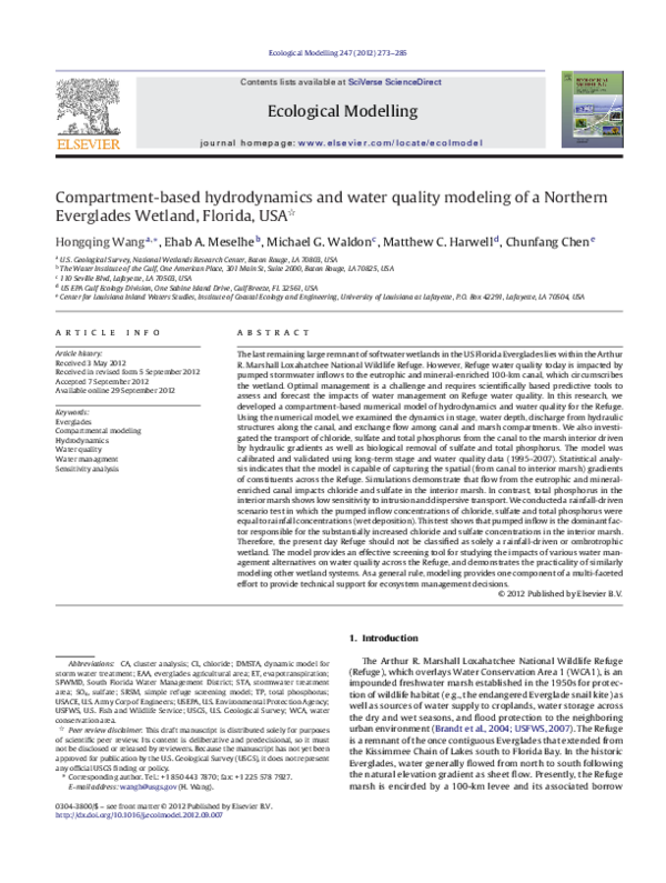
 Hongqing Wang