TESLA Report 2003-09 Tomasz Czarski, Ryszard Romaniuk, Krzysztof Pozjniak, Warsaw ELHEP Group ISE, Warsaw University of Technology TESLA, DESY, Hamburg Cavity Control System Models’ Simulations For TESLA Linear Accelerator ABSTRACT The fundamental knowledge contained in the previous paper “Cavity Control System Essential Modeling for TESLA Linear Accelerator” is applied for Matlabs’ Simulink implementation of the basic models for the cavity resonator. Elementary simulations of the cavity behavior are carried out and some experimental results for signals and power considerations are presented. 1. 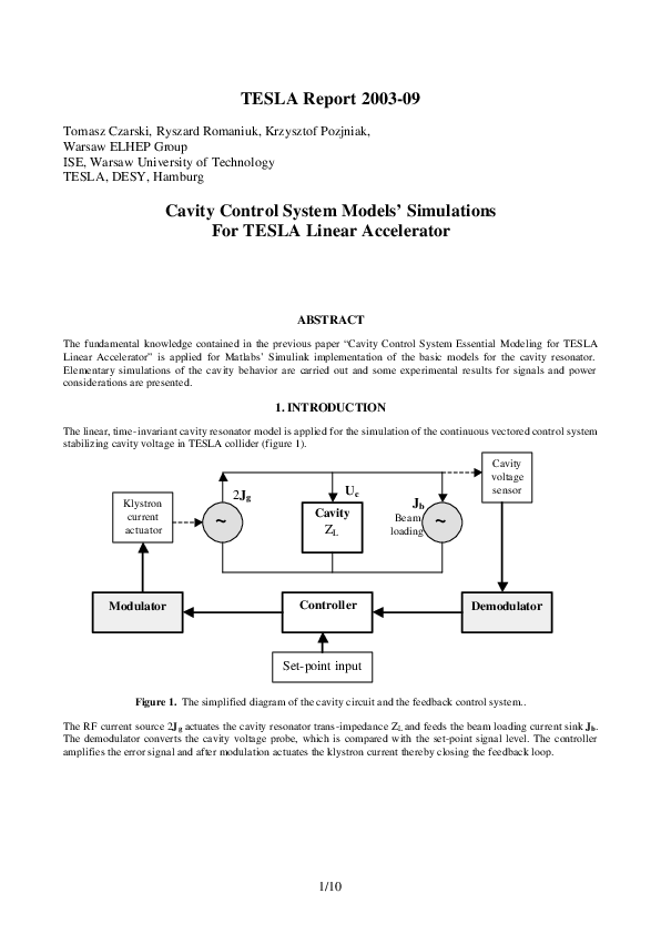INTRODUCTION The linear, time-invariant cavity resonator model is applied for the simulation of the continuous vectored control system stabilizing cavity voltage in TESLA collider (figure 1). Klystron current actuator Modulator Uc 2Jg ~ Cavity ZL Controller Cavity voltage sensor Jb Beam loading ~ Demodulator Set-point input Figure 1. The simplified diagram of the cavity circuit and the feedback control system.. The RF current source 2J g actuates the cavity resonator trans-impedance ZL and feeds the beam loading current sink J b. The demodulator converts the cavity voltage probe, which is compared with the set-point signal level. The controller amplifies the error signal and after modulation actuates the klystron current thereby closing the feedback loop. 1/10 The essential modeling of the system is based on the analytical signal idea. According to the generator’s constant frequency and due to a narrow resonator bandwidth, the cavity current and voltage signal is modeled as a generalized oscillation with its p/2 shifted Hilbert transform. After complex demodulation the low level frequency components inphase (I) and quadrature (Q) are detected and are used for controllers’ converting. Then after complex modulation the analytical signal again actuates the cavity. The complex cavity model relies on the fact that the parallel cavity linear transformation preserves the analytical signal for generalized oscillation, which can be used for demodulation. Double cavity model is implemented for a vector as well as for a phasor (in complex domain) representation of the analytical signal. However due to practical reasons: computation errors and long simulation time, it is implemented for the relatively high level signal and reasonably lower generator frequency. The complex cavity representation can be effectively simplified for signals with a narrow spectral range relative to the generator frequency close to cavity resonance pulsation. Composing modulation, cavity narrow bandwidth transformation and demodulation yields the approximated direct relation between input and output in-phase, quadrature components. Thus the resultant simple state space equation depends on the cavity bandwidth and detuning only. 2. MATLAB’S SIMULINK IMPLEMETATION of CAVITY CONTROL SYSTEM MODELS. 2.1 Vector representation for complex cavity system. The model of cavity control system applying the vector representation is composed in Simulink according to figure 2. Figure 2. The vector implementation of the complex cavity model. The parallel double cavity resonators transform the current analytical signal according to its LCR circuit transfer function. The vector demodulation converts the voltage signal to the in-phase and quadrature components. The controller matrix gain compares the signal with the required set-point signal level and amplifies the error. The vector 2/10 modulator creates the analytical signal according to the generator frequency (1MHz). The beam loading current sink subtracts its two mutually p/2 shifted pulsed structures components and the resultant current vector actuates the cavity. The beam loading is simulated by the pulse generator with the period of 10 µs and the width 1% of the period. The analytical signal is created only for the generator frequency Fourier component. This approximation is quite sufficient and the results for the cavity voltage response are illustrated in figure 3. As an example of the cavity behavior it is driven by the step signal on the resonance condition (detuning = 0) in the open loop mode. When the cavity field has reached half of its maximum (no reflection) the appropriate beam loading current is injected resulting in so called flattop operation. Figure 3. Cavity voltage response for step input signal and delayed beam loading current. 2.1 Phasor representation for complex cavity system. The model of the cavity control system applying the phasor representation is composed according to figure 2. 3/10 Figure 4. The phasor implementation of the complex cavity model. The complex cavity resonator transforms the analytical signal, which subsequently is demodulated to the phasor representation of the in-phase and quadrature components. The controller matrix gain compares the signal with the reference phasor and amplifies the error. The phasor modulator creates again the analytical signal, which loaded by the beam actuates the cavity. The beam loading is represented as the analytical signal for the generator frequency Fourier component only. As an example of the cavity behavior it is driven on three different resonance conditions in the open loop mode by step input, delayed beam loading and then turning off both signals (figure 5). 4/10 Figure 5. Cavity voltage response on resonance for frequencies: 1 MHz (cyan), 10 kHz (blue), 1 kHz (black) . 2.3 Control system implementation for state space cavity representation. The model of the cavity control system applying the state space representation is composed according to figure 2. Figure 6. The state space model implementation for the cavity control system. 5/10 The cavity is represented by its state space equation, which directly transforms the in-phase and quadrature signal components. The extracted beam loading current is related to its generator’s frequency component, which equals double value of the average current. The set-point input delivers the required signal level, which is compared to the actual cavity voltage. The proportional controller amplifies the signal error and closes the feedback loop. As an example of the cavity behavior it is driven on the resonance condition in the open loop mode by the step input signal (figure 7). Figure 7. Cavity voltage response and power monitoring for step input signal. 3. EXPERIMENTAL RESULTS OF SIMULATION. For the simulation purpose the only common “driving” Matlabs’ m.file is used to control three models implemented by the Simulink Toolbox. The main parameters of the models are available from this file and are combined in the table below. CAVITY parameters BW = 215; SET-POINT parameters bandwith [Hz] A = 1; signal relative amplitude det = 0; detuning [rad/s] v = 1/BW; time constant for filling [s] R = 1.5625; load resistance [Gom] T = 1.3e-3; pulse time [s] del = 1e -6; waveguide delay [s] ph= 0; phase of cavity voltage FEEDBACK parameters BEAM parameters loop = 0; open - loop = 0; closed - loop = 1 Beam = 8; beam current value [mA] k = 100; gain B_D = log(2)*v; beam delay time [s] lat = 4e -6; controller latency [s] 6/10 The three colored (red, blue, black) graphs comparison for three implemented models of the cavity system shows practically no visual difference of the cavity responses. As an example of the cavity behavior it is driven on resonance for three models by step input, delayed beam loading and then turning off both signals (figure 8) . Figure 8. Cavity models responses in open and closed loop mode and power monitoring for open loop mode. In the real operational condition the cavity system is driven in feedback mode according to its natural open loop response (figure 8). During the first stage of the operation the cavity is filled with constant forward power resulting in an exponential increase of the electromagnetic field. When transmitted power has reached the value of the forward power (no reflection) the beam loading current is injected resulting the steady-state flattop operation. Turning off both generator and beam current yields an exponential decay of the cavity field. The main reason of the cavity voltage destabilization is the resonance frequency changing caused by micrphonics and Lorentz force detuning. The detuning influence on the cavity behavior in the open loop mode is shown in figures 9, 10. [ MV ] [ MV ] Figure 9. Cavity voltage step response for different detuning. 7/10 [ MV ] [ MV ] Figure 10. Cavity voltage I/Q graph and power monitoring for different detuning. The feedback system stabilizes the cavity voltage at the expense of an additional forward power. The efficiency of the proportional controller during the operational condition for different gains at the constant detuning is shown in figure11. [ MV ] Figure 11. Cavity amplitude response and power monitoring for different controller gains (detuning = 400 Hz). 8/10 A high enough controller gain stabilizes the cavity voltage but the larger detuning the more power is required (fig. 12). Power monitoring [kW] 400 400 Hz 350 Phase of signal [rad] 1.8 1.6 forward power 400 Hz 1.4 300 300 Hz 1.2 300 Hz Phase [rad] power [kW] 250 200 Hz 200 detuning=0 Hz 1 0.8 150 0.6 transmitted power 200 Hz 100 0.4 50 0 0.2 0 0.5 1 time [s] 0 1.5 x 10 -3 detuning=0 Hz 0 0.5 1 time [s] 1.5 2 x 10 -3 Figure 12. Cavity power monitoring for different detuning (gain = 100) and phase shift during field decay. The high controller gain for the better accuracy and fast response of the cavity field is limited by the stability of the feedback system. The loop phase shift is the reason of the potential instability. The time delays caused by the waveguide and the digital controller latency are important contributions to the phase shift in the closed loop of the feedback system. The detuned cavity behavior for different loop delays at the constant controller gain shows figure 13. Delay 1 µs 3 µs 5 µs Figure 13. Cavity step response and I/Q graph for different loop delays (detuning =400Hz, controller gain = 200). 9/10 The detuned cavity behavior for different controller gains at the constant loop delay is shown in figure 14. Gain 50 100 200 Figure 14. Cavity step response and I/Q graph for different gains (detuning =400Hz, loop delay = 4 µs). 4. CONCLUSION. Using three models implemented in Matlabs’ Simulink Toolbox carries out the elementary simulations of the cavity resonator behavior. The approximate state space representation of the cavity control system is simple and useful for quite a satisfactory initial analysis of the system. The control feedback is very efficient to stabilize the detuned cavity voltage. However an additional forward power is necessary to obtain an accurate and fast cavity response. The controller gain is limited by the system instability mainly caused by the loop delay. In TESLA accelerator the auxiliary adaptive feed forward is applied to compensate the repetitive perturbations induced by the beam loading and dynamic Lorentz force detuning. The linear time-invariant cavity model is the first approximation of the resonator behavior. The next one should take into account the time-variant Lorentz force detuning during pulse operation and pass-band modes of the cavity. The design of a fast and efficient digital feedback controller is a challenging task and it is an important contribution to the optimization of TESLA accelerator. REFERENCES 1. T. Schilcher, “Vector Sum Control of Pulsed Accelerating Fields in Lorentz Force Detuned Superconducting Cavities”, Hamburg, August 1998. 2. T. Czarski, S. Simrock, K. Pozniak, R. Romaniuk “Cavity Control System Essential Modeling For TESLA Linear Accelerator”. Nov. 2002 3. W. Zabolotny, R. Romaniuk, K. Pozniak ...... “Design and Simulation of FPGA Implementation of RF Control System for Tesla Test Facility”. Warsaw University of Technology, Nov.2002. This paper was published in Proc. SPIE, vol. 5125 10/10