Proceedings of the 44th IEEE Conference on Decision and Control, and the European Control Conference 2005 Seville, Spain, December 12-15, 2005 TuA03.2 Stable Cooperative Surveillance Alvaro E. Gil, Kevin M. Passino and Jose B. Cruz, Jr. Dept. Electrical and Computer Engineering The Ohio State University 2015 Neil Avenue, Columbus, OH 43210-1272 Abstract— We consider a cooperative surveillance problem for a group of autonomous air vehicles (AAVs) that periodically receives information on suspected locations of targets from a satellite and then must cooperate to decide which AAV should search for each target. This cooperation must be performed in spite of imperfect inter-vehicle communications, less than full communication connectivity between vehicles, uncertainty in target locations, and imperfect vehicle search sensors. We represent the state of the search progress with a “search map,” and use an invariant set to model the set of states where there is no useful information on target locations. We show that the invariant set is exponentially stable for a class of cooperative surveillance strategies. Next, we show via simulations the impact of imperfect communications, imperfect vehicle search sensors, uncertainty in search locations, and pop-up suspected locations on performance. I. I NTRODUCTION Groups of possibly many AAVs of different types, connected via a communication network to implement a “vehicle network,” are technologically feasible and hold the potential to greatly expand operational capabilities at a lower cost. Cooperative control for navigation of such vehicle groups involves coordinating the activities of several agents so they work together to complete tasks in order to achieve a common goal. Here, we study how to perform a cooperative AAV surveillance task that involves two components: (i) search for stationary targets located in a region and (ii) reacting to “pop up” suspected target locations that are provided by a satellite (or other high-flying platform). There is a significant amount of current research activity focused on cooperative control of AAVs and some research directions in this field are identified in [1]. Solutions to general cooperative control problems can be obtained via solutions to vehicle route planning (VRP) problems [2]. Additional VRP-related work focusing on cooperative search and coordinated sequencing of tasks is in [3]-[6]. Using such approaches, significant mission performance benefits can be realized via cooperation in some situations, most notably when there is not a high level of uncertainty. One challenge in cooperative control problems is to overcome the effects of uncertainty so that benefits of cooperThe authors would like to thank AFRL/VA and AFOSR for financial support of the OSU Collaborative Center of Control Science (CCCS) where this research was performed (Grant F33615-01-2-3154). The authors would like to thank Andrew Sparks from AFRL for assistance in formulating the problem and Yong Liu for some initial collaboration on this problem. Correspondence should be directed to K. Passino at (614)-292-5716, fax: (614)-292-7596, passino@ece.osu.edu. A. Gil is now with Xerox Corporation, Webster, NY. 0-7803-9568-9/05/$20.00 ©2005 IEEE ation can still be realized. When uncertainty dominates the system, cooperative strategies will not be able to achieve the high level of coordination achieved in many of the abovementioned studies that assume perfect communications. The most that can be hoped for is to achieve some benefit from cooperation. Along these lines, recent work considering imperfect communications is found in [7]-[11]. Here, we continue along the lines of such work, but with a focus on cooperative surveillance when there are a variety of information flow constraints. Of all the current work in cooperative control, the most closely related to this study are the “persistent area denial (PAD)” [12], search theory [13], [14], and the “map-based approaches” in [15]-[18]. The main contributions of this paper are (i) the use of search-theoretic ROR maps [14] for the coordination of the search efforts of multiple AAVs, (ii) a novel characterization of cooperation objectives as stability properties of an invariant set, and (iii) the use of standard Lyapunov stability-theoretic methods for verification of cooperative control systems. In Section II the cooperative surveillance problem is formulated and modeled. The stability analysis is in Section III. Simulations are in Section IV. II. C OOPERATIVE S URVEILLANCE P ROBLEM F ORMULATION Suppose that there is a group of AAVs that performs surveillance of a given area and can use information from a satellite to pursue suspected locations in that area. Assume that the set of AAVs is given a number of targets to search for with their respective likely locations. AAVs must work together autonomously in order to try to maximize the probability of finding targets in the environment with minimal AAV effort. A. Discrete Event System Model The cooperative surveillance problem is modeled as a nonlinear discrete time asynchronous dynamic system [19] with the model G = (X , E, fe , g, Ev ). Here, X is the set of states. The set of events is denoted by E. State transitions are defined by fe : X −→ X , e ∈ E. The enable function, g, defines the occurrence of an event e by g : X −→ P(E)−{∅} being P(E) the power set of E. Note that fe is defined when e ∈ g. Let k ≥ 0 represent the time indices associated with both the states x(k) ∈ X and the enabled events e(k) ∈ g. 2182 Let Ev denote a set of “valid” event trajectories. Next, we define these for the cooperative surveillance problem. B. Vehicle Model Suppose that the mth AAV flies at a constant altitude and obeys a continuous time kinematic model given m m by the Dubin’s car [20], ẋm 1 (t) = v cos θ (t), ẋ2 (t) = m m m m v sin θ (t), θ̇ (t) = ωmax u (t) where x1 is its horizontal position, xm 2 is its vertical position, v is its forward (constant) velocity, θm is its heading direction, ωmax is its maximum angular velocity, and −1 ≤ um ≤ 1 is the steering input. Hence, um = +1(−1) stands for the sharpest possible turn to the right (respectively, left). The minimum turn radius for v the vehicle is R = ωmax . Rather than allow um (t) to be arbitrary, vehicles will either travel on the minimum turn radius or on straight lines that are the optimal paths from a vehicle’s current location and orientation to a desired location and orientation [21]. C. Search Environment and Targets The search environment is assumed to be rectangular with length L and width W . Divide the edge with length L into r ∈ Z+ segments and the edge with length W into s ∈ Z+ segments (Z+ is the set of the positive integers). This decomposes the search area into rs cells, each with a size of LW rs . Thus, there are NQ = rs discrete cells to search, and these cells are numbered so that the discretized search space is Q = {1, . . . , NQ }. It is assumed that all the AAVs know how the cells are numbered and hence know NQ . It is also assumed that there are NV AAVs that search for targets and let V = {1, . . . , NV } denote the set of vehicles. Assume that there are ND distinct valid stationary targets that the AAVs are searching for and let D = {1, . . . , ND } denote the set of targets. Suppose that the size of each target is considerably smaller than the size of each cell. Also, there could be more than one target located in one cell; however, it is assumed that all targets inside the same cell are separated in such a way that they can be detected by the sensors of the AAVs if, for example, they take enough “looks” at the cell. AAV sensors return information about the targets. Assume that the sensor of AAV m has a rectangular “footprint” with mL mW m m m + depth dm f1 = Nℓ r , width df2 = Nw s , Nℓ , Nw ∈ Z m m with Nℓ < r, Nw < s, and the distance from AAV m to the center of the footprint is denoted by dm s for all m ∈ V . Whenever a AAV is going to search a cell, it will approach this cell at an angle in the set {0, π2 , π, 3π 2 }. Due to sensor inaccuracies, it is assumed that searching a cell once may not result in finding a target even if it is there. Multiple searches of the same cell may be needed to find a target. In order to avoid detection by an adversary, AAVs turn their sensors on only when they have reached the desired orientation and location with respect to the center of the cell where the target is suspected to be located. Once a AAV takes a snapshot of the cell to be searched, the AAV will turn its sensor off until a new cell of interest is reached again. When targets are placed on the boundaries of the cells, it is assumed that when a cell is searched the search includes the left and lower boundaries of the cell, but it does not include the two endpoints lying opposite to where the boundaries join. This guarantees that the same object cannot be found by searching two different cells. D. The Rate of Return (ROR) Map Let pm j (q) be the AAV m ∈ V a priori probability that target j ∈ D is in cell q ∈ Q. These a priori probabilities must be specified by information gathering sources (e.g., the satellite or other high-flying platform). For simplicity, we assume here that pm j (q) = pj (q) for all m ∈ V so all AAVs get the same information. Let ℓm (q, k) ∈ {0, 1, . . .} be the number of looks (passes when a “snapshot” is taken) performed in cell q ∈ Q by AAV m ∈ V by time index k, which is a measure of the amount of search effort dedicated to cell q ∈ Q [14]. The AAVs share ℓm (q, k) for all m ∈ V , via inter-vehicle send/receive communications that may have arbitrary but finite delays. These delays should not be thought of as arising only from delays on, for instance, communication network links, but also from occlusions and sensing/communication range constraints, or temporary loss of a communication link between vehicles. The maximum delay between AAV ′ m′ and AAV m is known and equal to B m m ∈ Z+ . The unknown but bounded delay is modeled by a random choice ′ ′ ′ of τkm m , 1 ≤ τkm m ≤ B m m (with no assumption on the ′ underlying statistics). If m = m′ , then τkm m = 0 for all k since a vehicle knows its own information. Each AAV ′ ′ m ∈ V stores the values of ℓm (q, k − τkm m ) (i.e., the most recent information update that it has received from AAV ′ m′ ∈ V ) if the received ℓm (·) is greater than the current ′ value held by AAV m. Otherwise, AAV m discards ℓm (·) and keeps the old one (this event could arise due to the random nature of the inter-vehicle communication that could ′ result in message misordering of the ℓm (·) values sent by AAV m′ ). Each AAV m ∈ V in general only has up to date information on ℓm (q, k) (its own number of looks), not on the number of looks of other AAVs m′ = m that are out of ′ date by k − τkm m . AAV m ∈ V uses the latest information it
N ′ ′ has to form ℓ̂m (q, k) = mV′ =1 ℓm (q, k−τkm m ) its estimate of the total number of looks taken by all NV AAVs. Let Lm ⊂ V be a set that contains the AAVs m′ , m′ = m that have looked at cells q ∈ Q, possibly multiple times ′ denoted by nm (ℓm (q, k)) ≥ 1, between the time when AAV m decides to perform an additional look at target j in cell q and the time when AAV m actually receives the new looks. Let Qm ⊂ Q be the set held by AAV m, which represents the cells that have been visited by AAV m′ ∈ Lm ⊂ V . Let Cm denote the set of cells covered by the sensor footprint of AAV m. Define for each   the mset mof “local” events m, Lm , Qm , Cm Cm , , e AAV m as e1m, L , Q , em, 3 2 m m L ,Q where em, = “Reception of looks at q ∈ 1 Cm m ′ = Q from m ∈ Lm ,” em, 2 m m “AAV mm sensor on for cells q ∈ Cm ,” e3m, L , Q , Cm = m L ,Q Cm occur simultaneously” so that the and em, “em, 2 1 set of events of the system such that e(k) ∈ g is any subset 2183 and an additional look will be executed by AAV m in cell q. Clearly AAV m would like to place search effort in cells where this quantity is the largest. of E =P N V  m=1  L em, 1 m , Qm Cm , , em, 2 m m e3m, L , Q , Cm   E. Detection of Targets − {∅} (1) that contains all the elements of the right side of Equation (1) except that only one of the three types of local events can be in any event e ∈ E. Thus, the enable function g allows the occurrence of a set of possible events at the same time. Let am j,q > 0 be a parameter that is proportional to the sensor capabilities of AAV m for target j in cell q. Let m πj,q ∈ (0, 1] be the probability that AAV m detects target j in cell q on a single look, given that target j is in cell q. ′ m′ Assume that AAV m knows each πj,q and am j,q from AAV m′ , m′ = m, m ∈ V . Let the detection function [13], [14], m bm j (ℓ̂ (q, k)), be the conditional probability of detecting target j in cell q by AAV m, given that target j is in cell q. If each cell look has an independent probability of finding m the target, then the detection function is bm j (ℓ̂ (q, k)) =  NV m′ m m′ m′ ′ ) m aj,q ℓ (q,k−τk . Since ℓ̂m (q, k) is an ) 1 − m′ =1 (1 − πj,q m m estimate, bj (ℓ̂ (q, k)) should be thought of as an estimate of the probability j ∈ D was found. AAV m ∈ V will use this estimate to decide where to search. The cost for searching for target j with ℓm (q, k) looks is m m defined as cm j (ℓ (q, k)) = c ℓ (q, k) where c > 0 is the cost of a single search. Note that the cost of one look at target j m in cell q is given by γjm (ℓm (q, k) + 1) = cm j (ℓ (q, k) + 1) − m m cj (ℓ (q, k)) = c. In our simulations we will incorporate the cost of moving to a location as part of the decision making; however, in our theory c is independent of distance. It is a future direction to incorporate distance into c for the theory. Let β̂jm (ℓ̂m (q, k) + 1) be the mth AAV’s probability of failing to detect target j on the first ℓ̂m (q, k) looks in cell q and succeeding on the ℓ̂m (q, k)th + 1 look (where 1 in the expression ℓ̂m (q, k)+1 is the look that AAV m is considering whether to take), given that target j is in cell q and assuming that no other AAVs look at cell q before AAV m does. The variable β̂jm (ℓ̂m (q, k) + 1) is m m m β̂jm (ℓ̂m (q, k) + 1) = b̂m j (ℓ̂ (q, k) + 1) − bj (ℓ̂ (q, k)) (2) m where b̂m j (ℓ̂ (q, k) + 1) is the estimated detection function computed by time index k when AAV m will perform an additional look in cell q. It is an estimated value since there exists the possibility that new number of looks by AAVs m′ = m could be taken before AAV m takes the look at cell q, which would change the expression shown in Equation (2). The rate of return (ROR) [14] in cell q for target j and AAV m can be defined in order to determine the benefit that AAV m obtains at time index k when an additional look will be performed to find target j in cell q. Hence, pj (q)β̂jm (ℓ̂m (q,k)+1) m ρ̂m which gives the ratio j (ℓ̂ (q, k) + 1) = γjm (ℓm (q,k)+1) of the increase in probability to the increase in cost when ℓ̂m (q, k) looks for target j have been performed in cell q Note that when AAV m finds target j, this AAV makes pj (q) = 0 and communicates this information to the satellite, which broadcasts to all the AAVs the target that has been found. Hence, all the AAVs make their respective pj (q) = 0 as well. By making pj (q) = 0, the AAV that found target j along with the ones that received this information are forcing their ROR maps to be equal to zero. This means that this target is no longer of interest to these AAVs. Below, in our stability analysis we will assume either that targets are not found, or that if one is then this corresponds to a state perturbation and hence is viewed as restarting the process. F. Percentage Rate of Return (PROR) Map Next, we introduce what we call the “percentage rate of m return” (PROR) map ρm j (ℓ̂ (q, k) + 1), which is the ratio of the percentage change in probability to the percentage change in cost when ℓ̂m (q, k) looks for target j have been performed by AAV m in cell q and an additional look will m be executed by AAV m in cell q. Hence, ρ̂j (ℓ̂m (q, k)+1) = m pj (q)β̂jm (ℓ̂m (q,k)+1)cm j (ℓ (q,k)) . Note that there are differences between the PROR and the ROR map cases. However, as in the ROR case, AAV m would like to place search effort in m cells where ρ̂j (ℓ̂m (q, k) + 1) is the largest. m m m bm j (ℓ̂ (q,k))γj (ℓ (q,k)+1) G. Cooperative Surveillance Strategies The ROR maps will be used in the strategies; however, the PROR maps can also be used by replacing each variable m ρ̂m j (·) by ρ̂j (·). Next, one choice for search strategies is discussed. This strategy commands a AAV to search for the target in the cell with the highest ROR map that is obtained using both its own number of looks and the possibly outdated number of looks received from other AAVs through communications. In particular, the search decision for AAV m ∈ V at time index k is q ∗ (m, k) ∈ Q which defines the cell it will search in next. Here, the strategy “go to the cell where a single target is most likely to be present” is chosen as    ρ̂m q ∗ (m, k) = arg max (3) ℓ̂m (q, k) + 1 j j∈D, q∈Q and once AAV m reaches the location where cell q ∗ (m, k) is, it searches for all target types in it (break ties arbitrarily or via going to the closest cell). If AAV m receives a new look value for cell q from any AAV m′ = m while AAV m is heading to cell q, this could lead AAV m to cell q ′ = q next if the ROR map of cell q is not the maximizer at the reception time of the new information. Thus, AAV decision reconsiderations about the current maximum benefit are allowed in this framework. 2184 A policy “go look in any cell such that any target is most likely to be present” can be defined as follows ⎧ ⎫ ⎨ ⎬   m ρ̂m (q, k) + 1 (4) q ∗ (m, k) = arg max ℓ̂ j q∈Q ⎩ ⎭ j∈D where ties are broken arbitrarily or by going to the closest cell. Note that both policies only rely on information at time index k that is locally available at AAV m; hence, they can be implemented in a distributed fashion. Also, both policies are computationally simple. H. Distributed ROR Map Updates The cooperative AAV surveillance problem can be viewed as being composed of NV subsystems and AAV m ∈ V is associated with the mth subsystem. Let the state ND NQ where xm (k) = of AAV m be xm (k) ∈ R+  ⊤ m m m ρm is the vector that 1 (ℓ̂ (1, k)), . . . , ρND (ℓ̂ (NQ , k)) contains all the ROR map values that AAV m holds by time index k. Let x(k) = [x1 (k)⊤ , . . . , xNV (k)⊤ ]⊤ = X ∈ NV ND NQ be the states of the system at time index k. R+ Let the sequence {x(k − 1)} ∈ X N denote the state trajectory such that x(k) = fe(k) (x(k − 1)) for some e(k) ∈ g(x(k)) for all k ≥ 0. Define the sequence {e(k)} ∈ E N as an event trajectory such that there exists a state trajectory, {x(k −1)} ∈ X N , where e(k) ∈ g(x(k)) for every k. The set of all event trajectories is denoted by E ⊂ E N . Since each ′ ′ AAV m stores ℓm (q, k − τkm m ) from any AAV m′ = m when it is greater than the current value that AAV m holds, the set Ev ⊂ E can account for these events and it prunes the set E. An ROR map will be updated at anytime when an event e(k) ∈ g(x(k)) occurs using the state transition function fe . Thus, there are three ways of updating the ROR maps for each AAV corresponding to the three event types. An ROR map update is performed by AAV m when it is not visiting a cell of interest and receives one ormmore number m, L (q,k), Qm (k) of looks from AAV m′ = m. For event e1 ∈ e(k) ∈ g(x(k)), components of xm (k) with q ∈ Qm (k) m m m m have ρm j (ℓ̂ (q, k)) = ρj (ℓ̂ (q, k − 1))h(ℓ (q, k)) where ′′  m m′′ m′′ am ) j,q n (ℓ (q,k)) . The h(ℓm (q, k)) = m′′ ∈Lm (q,k) (1−πj,q m, C (k) ∈ e(k) ∈ g(x(k)) forces occurrence of event e2 m m ( ℓ̂ (q, k)) so that the components of AAV m to update ρm j m m xm (k) with q ∈ Cm (k) have ρm ( ℓ̂ (q, k)) = ρm j j (ℓ̂ (q, k − m m m, L (q,k), Q (k), Cm (k) m am ∈ 1))(1 − πj,q ) j,q . When an event e3 m e(k) ∈ g(x(k)) occurs, the components of x (k) with  m m m q ∈ Cm (k) Qm (k) have ρm j (ℓ̂ (q, k)) = ρj (ℓ̂ (q, k − m m am 1))(1 − πj,q ) j,q h(ℓ (q, k)), the components with q ∈ m m m (Cm (k) − Qm (k)) have ρm j (ℓ̂ (q, k)) = ρj (ℓ̂ (q, k − m am j,q 1))(1 − πj,q ) , while the components of xm (k) with m m m q ∈ (Qm (k) − Cm (k)) have ρm j (ℓ̂ (q, k)) = ρj (ℓ̂ (q, k − m 1))h(ℓ (q, k)). If the PROR approach is used, then map updates can also be derived as above. III. S TABILITY A NALYSIS Let H = {1, . . . , NV ND NQ }. If z is a vector, then (z)i denotes the ith component of this vector. Let Xε = {x(k) ∈ X : 0 ≤ (x(k))i ≤ ε, for all i ∈ H} , ε > 0 be the set that holds the AAVs’ ROR map values that are less than or equal to ε at time index k. Typically, ε is chosen to be small so that, since the search cost c is fixed, the set Xε characterizes when the probability that further looks of any cell are unlikely to find a target. Hence, when the state is in Xε the group of AAVs has “used up” the information about likely target locations that was provided initially by the satellite. Initially, the AAVs by themselves are assumed to have no target location information (so the state is in Xε ) and then at k = 0 the satellite provides pj (q) and this corresponds to a perturbation from the Xε set. Let d(x(k), Xε ) : X → R+ denote a metric on R+ d(x(k), Xε ) = inf{max{|(x(k))i − (x′ )i |}} (5) i for all i ∈ H, x′ ∈ Xε . We are interested in showing that the cooperative surveillance strategy will drive perturbations from Xε back into Xε . To do that, we first introduce a lemma that shows that every component (x(k))i will get closer to the set Xε several time indices after k. The derivation of these time indices after k depends on temporal (i.e., delays) and spatial (i.e., the position of all the AAVs at time index k, and the density of the suspected target locations) characteristics of the cooperative surveillance problem. Finally, we use the result obtained in the lemma to show that Xε is exponentially stable. ′ Lemma 3.1: Let Nqm be the number of times that AAV ′ m′ visits cell q between time indices k and k + C(Nqm ). Let q ℓ be the last cell visited by AAV m at time index ′ k + C(Nqm ). If we define a Lyapunov function V (k) = maxi {|(x(k))i − ε|} and NV AAVs use any cooperative surveillance strategy that satisfies Equation (3), then there exists a function ⎡ NQ ′ C(Nqm ) = NQ N V − NV + 1 + m′ =m ′ + q=q
′ ⎣ Nqm ′ q=1 ⎤ Nqm (NV − 1) + Nqm
(NV − 2)⎦ (6) ′ that guarantees that V (k + C(Nqm )) < V (k). ′ Remark 1 A lower bound for C(Nqm ) could be obtained in Equation (6) for the special case where every AAV visits ′ every cell once (i.e., Nqm = 1 for all m′ ∈ V, q ∈ Q) and the delays are so large so that Equation (6) is now C(1) = NQ NV . Remark 2 A similar result to Remark 1 can be obtained for the case when the delays are small and when every AAV m visits a differentgroup of cells between k and ′ ′ ′ k +C(Nqm ) such that Qm Qm c c = {∅} for all m = m and  NV m m m=1 Qc = Q. Assume that Nq = 1, and that every AAV m′ = m receives this information. Using Equation (6) for 2185 this particular case, C(1) = NV NQ . The benefit of sharing information is shown in this particular scenario since every AAV does not have to visit every cell, which minimizes AAV’s fuel expenditure. Theorem 3.2: If NV AAVs use any cooperative surveillance strategy that satisfies Equation (3), then the set Xε is invariant and exponentially stable in the large w.r.t. Ev . For c1 = c2 = 1, 0 < σ < 1, and 0 < c3 = max{π a , 1 − max {(1 − π)a , σ}} < c2 , Equations (7) and (8) are satisfied c1 d(x(k), Xε ) ≤ V (k) ≤ c2 d(x(k), Xε ) ′ V (k + C(Nqm )) − V (k) ≤ −c3 d(x(k), Xε ) (7) each ROR map covered by the sensor footprint in its previous projection length before making any decision about the cell to be visited next. Let L = 10000 meters, W = 10000 meters, r = s = 100, NV = 3, v = 150 meters/sec, R = 800 meters, m m dm f1 = df2 = 500 meters, ds = 400 meters, ND = 4 (i.e., four suspected areas in the environment, see Figure 1), ′ m′ = 0.8, am πj,q j,q = 0.9 (e.g., imperfect sensors), for all m ∈ V, j ∈ D, q ∈ Q, the sampling time Ts = 0.1 sec., and the simulation length of 600 sec. All these above parameters are used in the simulations unless otherwise stated. (8) for all x(0) ∈ X , k ≥ 0 with 0 < c3 /c2 < 1 for some ′ specified C(Nqm ) > 0. Remark 3 The ROR map values will enter faster into the invariant set when the probability of detecting targets in cells on one single look is close to 1 (i.e., π = π ≈ 1) and the AAVs’ group possesses high quality sensors (i.e., a ≫ 1) for all m ∈ V, j ∈ D, q ∈ Q (see the variables in c3 ). Remark 4 An analogous stability analysis can be carried out for the strategy shown in Equation (4). Moreover, an analysis can be conducted for showing the stability of Xε when PROR maps are used. Remark 5 A “noncooperative” case can be defined if the AAVs do not communicate with each other so they do not share the number of looks. It can be shown that the performance of the cooperative strategies can be no worse than the noncooperative ones under some special cases. IV. S IMULATIONS Here, two simulation are shown in this section. Travel distances between cells are considered for each AAV at each decision time. Let xq = [xq1 , xq2 ]⊤ denote the coordinates in the (xq1 , xq2 ) plane of the center of the q th cell. Let ds (xm (k), xq ) > 0 be the minimum distance that AAV m must travel at index k from its current location and m m ⊤ to take a orientation xm (k) = [xm 1 (k), x2 (k), θ (k)] snapshot at cell q. Notice that since all AAVs are moving all the time, it is not possible to have ds (xm (k), xq ) = 0 due to if an AAV needs to take two consecutive snapshots of the same cell, then this particular AAV will travel a distance, different from zero, determined by the path generated by Dubin’s car. The cooperative strategy defined in Equa∗ tion (3) is modified  for the nonplanning case as q (m,k) = 1 m m arg maxj∈D, q∈Q ρ̂j ℓ̂ (q, k) + 1 + ds (xm (k),xq ) . Consider, for the cooperative strategy with planning, that AAV m plans to visit a sequence of cells next at index k. The planning cooperative surveillance strategy for AAV m is made over the ROR maps. Suppose now that the AAVs share the cells included in the planning horizon along with the number of looks for all m ∈ V , via inter-vehicle communications with arbitrary but finite delays. 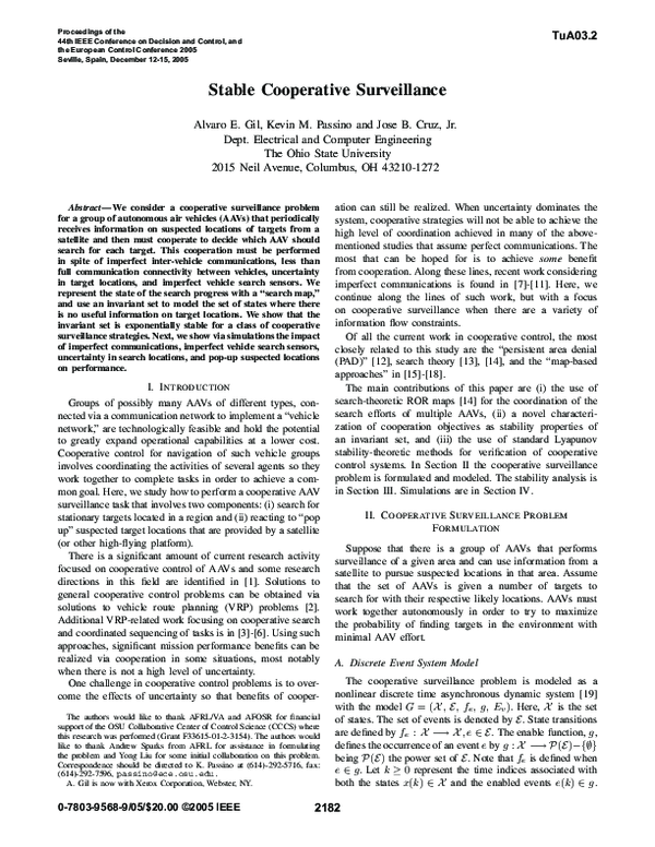Thus, each AAV m first flattens out each ROR map associated with each cell contained in the projection length of each AAV m′ = m, and then it further flattens out, except in the first projection, Suspected locations for target 1 Suspected locations for target 4 AAVs Suspected locations for target 3 Suspected locations for target 2 Fig. 1. Initial positions and orientations of AAVs and suspected locations of targets. AAVs are labeled 1 up to 3 from left to right. A. Performance in the Presence of Pop-Up Suspected Locations The behavior of the cooperative strategies with planning is shown in this section when some suspected locations pop-up when the group of AAVs have already begun the mission. The same parameters mentioned above are used in this simulation except the following: The suspected area of targets 1 and 2 are available to all the AAVs at the beginning of the simulation, while the suspected areas of targets 3 and 4 pop up at time 230 sec. Moreover, the horizon length for ′ each AAV is 3 and the communication delays, 1 ≤ τkm m ≤ 3 sec., are fixed randomly between AAVs during the mission. The trajectories of the AAVs are shown in Figure 2. Note (a) Mission performance without targets 3 and 4 (b) Mission performance with targets 3 and 4 Fig. 2. Performance of cooperative surveillance strategies in the presence of pop-up suspected locations. that the group of AAVs focus their effort in the suspected locations of targets 1 and 2 since the beginning of the mission and up to the 230 sec. (see Figure 2(a)). Thus, the suspected locations of targets 3 and 4 pop-up 230 sec. after the mission has begun and the group of AAVs focus on those new areas and finally make some visits to the location where targets 1 and 2 might be (see Figure2(b)). 2186 B. Influences of Communication Delays and Plan Horizons We focus here on the AAVs’ performance when both nonplanning and planning strategies are used for the cooperative surveillance in a mission. We would like to obtain conditions under which it is best to plan over the maps and when it is best not to do it in the presence of communications delays. We run a Monte Carlo simulation with the following values: ′ the maximum delay in a range B m m ∈ {0.2, 1, 3, 5, 10, 20} ′ ′ sec. for each m, m , m = m , and a projection lengths range of P ∈ {1, 3, 5}. Each delay-projection length case consists of 35 simulations where the communication delays are randomly generated in each of these simulations such ′ ′ that 1 ≤ τkm m ≤ B m m for all m = m′ . The number of simulations for each delay-projection length combination was chosen such that the standard deviation of the performance measures did not change significantly and settled to a relatively small constant value beyond 35 simulations. We use the metric defined in Equation (5) as a way to evaluate performance. We compute the average of the average of the metric at each delay-projection length case with ε = 10−4 . We also compute the maximum of the average of this quantity over the entire simulation run. Figure 3(a) shows the performance of both the nonplanning and planning case for the average of the average of the metric. Notice that the 3 11 3 x 10 11 x 10 10.5 10.5 10 10 9.5 9 9.5 8.5 9 8 Nonplanning 1 look ahead 2 looks ahead 3 looks ahead 4 looks ahead 5 looks ahead 6 looks ahead 7.5 7 0 2 4 6 8 10 delays(sec. ) 12 14 (a) Average of average of metric Fig. 3. 16 18 Nonplanning 1 look ahead 2 looks ahead 3 looks ahead 4 looks ahead 5 looks ahead 6 looks ahead 8.5 20 8 0 2 4 6 8 10 delays(sec. ) 12 14 16 18 20 (b) Maximum of average of metric Performance measures of the nonplanning and planning case. performance of the nonplanning case stays almost constant for the range of communication delays considered in the simulation. For the planning case, the performance decreases for small delays, except for the “one look ahead” case, due to the fact that most of the time the AAVs make decisions at the same time, which results in a worst performance for the bounded delay equals to 0.2 second. Then, all the performances increase almost steadily for larger delays than 1 second. It is important to highlight that it is worthwhile to consider large projection lengths for small communication delays. However, when the communication delays are large then the value of planning ahead over the maps is not useful (e.g., note, for instance, how the performance for all the projection lengths have almost the same value for a delay of 20 seconds). Moreover, if we run the simulation for larger delays, then the performance of the planning case will eventually be equal to the nonplanning case. Figure 3(b) shows the performance for both the nonplanning and planning case when the maximum of the average of the metric is used as a performance measure. Notice that it is better to use a nonplanning strategy for the AAVs instead of some planning strategies for delays greater than 3 seconds. However, all the planning strategies are superior than the nonplanning one for delays less than 3 seconds. Note that when the delay is equal to 20 seconds all the performances are about the same so it is better to use a nonplanning strategy for large delays. R EFERENCES [1] P. Chandler and M. Pachter, “Research issues in autonomous control of tactical UAVs,” in Proc. of the ACC, Philadelphia, PA, 1998, pp. 394–398. [2] G. Laporte, “The vehicle routing problem: An overview of the exact and approximate algorithms,” European Journal of Operational Research, vol. 59, pp. 345–358, 1992. [3] J. Bellingham, A. Richards, and J. How, “Receding horizon control of autonomous aerial vehicles,” in Proc. of the ACC, Anchorage, AK, 2002, pp. 3741–3746. [4] W. Li and C. G. Cassandras, “Stability properties of a receding horizon controller for cooperating UAVs,” in Proc. IEEE CDC, Paradise Island, Bahamas, 2004, pp. 2905–2910. [5] R. Beard, T. McLain, and M. Goodrich, “Coordinated target assignment and intercept for unmanned air vehicles,” in Proc. IEEE Int. Conference on Robotics and Automation, Washington, DC, 2002, pp. 2581–2586. [6] M. G. Earl and R. D’Andrea, “Iterative MILP methods for vehicle control problems,” in Proc. IEEE CDC, Paradise Island, Bahamas, 2004, pp. 4369–4374. [7] D. A. Castanon and C. Wu, “Distributed algorithms for dynamic reassigment,” in Proc. IEEE CDC, Maui, HI, 2003, pp. 13–18. [8] R. W. Beard and T. W. McLain, “Multiple UAV cooperative search under collision avoidance and limited range communication constraints,” in Proc. IEEE CDC, Maui, HI, 2003, pp. 25–30. [9] A. E. Gil, K. M. Passino, S. Ganapathy, and A. Sparks, “Cooperative scheduling of tasks for networked uninhabited autonomous vehicles,” in Proc. IEEE CDC, Maui, HI, 2003, pp. 522–527. [10] J. Finke, K. M. Passino, and A. Sparks, “Cooperative control via task load balancing for networked uninhabited autonomous vehicles,” in Proc. IEEE CDC, Maui, HI, 2003, pp. 31–36. [11] B. J. Moore and K. M. Passino, “Coping with information delays in the assignment of mobile agents to stationary tasks,” in Proc. IEEE CDC, Paradise Island, Bahamas, 2004. [12] Y. Liu and J. B. Cruz, “Coordinating networked uninhabited air vehicles for persistent area denial,” in Proc. IEEE CDC, Paradise Island, Bahamas, 2004, pp. 3351–3356. [13] B. O. Koopman, Search and Screening, 2nd ed. Elmsford, New York: Pergamon Press, 1980. [14] L. D. Stone, Theory of Optimal Search, 2nd ed. Arlington, Virginia: Academis Press, 1989. [15] K. M. Passino et al., “Cooperative control for autonomous air vehicles,” in Cooperative Control and Optimization, R. Murphey and P. M. Pardalos, Eds. Kluwer Academic Publishers, 2002, vol. 66, pp. 233–271. [16] M. Baum and K. Passino, “A search-theoretic approach to cooperative control for uninhabited air vehicles,” in AIAA GNC Conference, Monterrey, CA, Aug. 2001. [17] J. Hespanha and H. Kizilocak, “Efficient computation of dynamic probabilistic maps,” in Proceedings of the 10th Mediterranean Conference on Control and Automation, Lisbon, Portugal, July 2002. [18] S. Ganapathy and K. Passino, “Agreement strategies for cooperative control of uninhabited autonomous vehicles,” in Proc. of the ACC, Denver, CO, 2003, pp. 1026–1031. [19] K. Passino and K. Burgess, Stability Analysis of Discrete Event Systems. John Wiley and Sons, Inc., NY, 1998. [20] L. Dubins, “On curves of minimal length with a constraint on average curvature, and with prescribed initial and terminal position,” American Journal of Math, vol. 79, pp. 497–516, 1957. [21] H. J. Sussman and G. Tang, “Shortest paths for the Reeds-Shepp car: a worked out example of the use of geometric techniques in nonlinear optimal control,” Rutgers University, New Brunswick, NJ, Tech. Rep. SYCON-91-10, 1991. 2187