C∗ -ALGEBRAS OVER TOPOLOGICAL SPACES:
THE BOOTSTRAP CLASS
arXiv:0712.1426v3 [math.KT] 11 Dec 2008
RALF MEYER AND RYSZARD NEST
Abstract. We carefully define and study C∗ -algebras over topological spaces,
possibly non-Hausdorff, and review some relevant results from point-set topology along the way. We explain the triangulated category structure on the
bivariant Kasparov theory over a topological space and study the analogue of
the bootstrap class for C∗ -algebras over a finite topological space.
1. Introduction
If X is a locally compact Hausdorff space, then there are various equivalent
characterisations of what it means for X to act on a C∗ -algebra A. The most
common definition uses an essential ∗ -homomorphism from C0 (X) to the centre of
the multiplier algebra of A. An action of this kind is equivalent to a continuous
map from the primitive ideal space Prim(A) of A to X. This makes sense in general:
A C∗ -algebra over a topological space X, which may be non-Hausdorff, is a pair
(A, ψ), where A is a C∗ -algebra and ψ : Prim(A) → X is a continuous map. One of
the purposes of this article is to discuss this definition and relate it to other notions
due to Eberhard Kirchberg and Alexander Bonkat [4, 10].
An analogue of Kasparov theory for C∗ -algebras over locally compact Hausdorff
spaces was defined already by Gennadi Kasparov in [9]. He used it in his proof
of the Novikov conjecture for subgroups of Lie groups. Kasparov’s definition was
extended by Eberhard Kirchberg to the non-Hausdorff case in [10], in order to
generalise classification results for simple, purely infinite, nuclear C∗ -algebras to
the non-simple case. In his thesis [4], Alexander Bonkat studies an even more
general theory and extends the basic results of Kasparov theory to this setting.
This article is part of an ongoing project to compute the Kasparov groups
KK∗ (X; A, B) for a topological space X and C∗ -algebras A and B over X. The aim
is a Universal Coefficient Theorem in this context that is useful for the classification
programme. At the moment, we can achieve this goal for some finite topological
spaces (see [16]), but the general situation, even in the finite case, is unclear.
Here we describe an analogue of the bootstrap class for C∗ -algebras over a topological space. Although we also propose a definition for infinite spaces in §4.4, most
of our results are limited to finite spaces.
Our first task is to clarify the definition of C∗ -algebras over X; this is the main
point of Section 2. Our definition is quite natural, but more restrictive than the
definitions in [4, 10]. The approach there is to use the map O(X) → O(Prim A)
induced by ψ : Prim(A) → X, where O(X) denotes the complete lattice of open
subsets of X. If X is a sober space – this is a very mild assumption that is also made
under a different name in [4, 10] – then we can recover it from the lattice O(X),
and a continuous map Prim(A) → X is equivalent to a map O(X) → O(Prim A)
that commutes with arbitrary unions and finite intersections.
2000 Mathematics Subject Classification. 19K35, 46L35, 46L80, 46M20.
1
�2
RALF MEYER AND RYSZARD NEST
The definition of the Kasparov groups KK∗ (X; A, B) still makes sense for any
map O(X) → O(Prim A) (in the category of sets), that is, even the restrictions
imposed in [4,10] can be removed. But such a map O(X) → O(Prim A) corresponds
to a continuous map Prim(A) → Y for another, more complicated space Y that
contains X as a subspace. Hence the definitions in [4, 10] are, in fact, not more
general. But they complicate computations because the discontinuities add further
input data which must be taken into account even for examples where they vanish
because the action is continuous.
Since the relevant point-set topology is widely unknown among operator algebraists, we also recall some basic notions such as sober spaces and Alexandrov
spaces. The latter are highly non-Hausdorff spaces – Alexandrov T1 -spaces are
necessarily discrete – which are essentially the same as preordered sets. Any finite
topological space is an Alexandrov space, and their basic properties are crucial
for this article. To get acquainted with the setup, we simplify the description of
C∗ -algebras over Alexandrov spaces and discuss some small examples. These rather
elementary considerations appeared previously in the theory of locales.
In Section 3, we briefly recall the definition and the basic properties of bivariant
Kasparov theory for C∗ -algebras over a topological space. We omit most proofs
because they are similar to the familiar arguments for ordinary Kasparov theory
and because the technical details are already dealt with in [4]. We emphasise the
triangulated category structure on the Kasparov category over X because it plays
an important role in connection with the bootstrap class.
In Section 4, we define the bootstrap class over a topological space X. If X is
finite, we give criteria for a C∗ -algebra over X to belong to the bootstrap class.
These depend heavily on the relation between Alexandrov spaces and preordered
sets and therefore do not extend directly to infinite spaces.
We define the X-equivariant bootstrap class B(X) as the localising subcategory
of the Kasparov category of C∗ -algebras over X that is generated by the basic
objects (C, x) for x ∈ X, where we identify x ∈ X with the corresponding constant
map Prim(C) → X. Notice that this is exactly the list of all C∗ -algebras over X
with underlying C∗ -algebra C.
We show that a nuclear C∗ -algebra (A, ψ) over X belongs to the X-equivariant
bootstrap class if and only if its “fibres” A(x) belong to the usual bootstrap class
for all x ∈ X. These fibres are certain subquotients of A; if ψ : Prim(A) → X is a
homeomorphism, then they are exactly the simple subquotients of the C∗ -algebra A.
The bootstrap class we define is the class of objects where we expect a Universal Coefficient Theorem to hold. If A and B belong to the bootstrap class, then
an element of KK∗ (X; A, B) is invertible if and
� only if it is �fibrewise invertible on
K-theory, that is, the induced maps K∗ A(x) → K∗ B(x) are invertible for all
x ∈ X. This follows easily from our definition of the bootstrap class. The proof of
our criterion for a C∗ -algebra over X to belong to the bootstrap class already provides a spectral sequence that computes KK∗ (X; A, B) in terms of non-equivariant
Kasparov groups. Unfortunately, this spectral sequence is not useful for classification purposes because it rarely degenerates to an exact sequence.
We call a C∗ -algebra over X tight if the map Prim(A) → X is a homeomorphism.
This implies that its fibres are simple. We show in Section 5 that any separable nuclear C∗ -algebra over X is KK(X)-equivalent to a tight, separable, nuclear, purely
infinite, stable C∗ -algebra over X. The main issue is tightness. By Kirchberg’s
classification result, this model is unique up to X-equivariant ∗ -isomorphism. In
this sense, tight, separable, nuclear, purely infinite, stable C∗ -algebras over X are
classified up to isomorphism by the isomorphism classes of objects in a certain triangulated category: the subcategory of nuclear C∗ -algebras over X in the Kasparov
�C∗ -ALGEBRAS OVER TOPOLOGICAL SPACES: THE BOOTSTRAP CLASS
3
category. The difficulty is to replace this complete “invariant” by a more tractable
one that classifies objects of the – possibly smaller – bootstrap category B(X) by
K-theoretic data.
If C is a category, then we write A ∈∈ C to denote that A is an object of C – as
opposed to a morphism in C.
2. C∗ -algebras over a topological space
We define the category C∗ alg(X) of C∗ -algebras over a topological space X. In
the Hausdorff case, this amounts to the familiar category of C0 (X)-C∗ -algebras. For
non-Hausdorff spaces, our notion is related to another one by Eberhard Kirchberg.
For the Universal Coefficient Theorem, we must add some continuity conditions to
Kirchberg’s definition of C∗ alg(X). We explain in §2.9 why these conditions result
in essentially no loss of generality. Furthermore, we explain briefly why it is allowed
to restrict to the case where the underlying space X is sober, and we consider some
examples, focusing on special properties of finite spaces and Alexandrov spaces.
2.1. The Hausdorff case. Let A be a C∗ -algebra and let X be a locally compact
Hausdorff space. There are various equivalent additional structures on A that
turn it into a C∗ -algebra over X (see [17] for the proofs of most of the following
assertions). The most common definition is the following one from [9]:
Definition 2.1. A C0 (X)-C∗ -algebra is a C∗ -algebra A together with an essential
∗
-homomorphism ϕ from C0 (X) to the centre of the multiplier algebra of A. We
abbreviate h · a := ϕ(h) · a for h ∈ C0 (X).
A ∗ -homomorphism f : A → B between two C0 (X)-C∗ -algebras is C0 (X)-linear
if f (h · a) = h · f (a)�for all h ∈ C0 (X), a ∈ A.
Let C∗ alg C0 (X) be the category of C0 (X)-C∗ -algebras, whose morphisms are
the C0 (X)-linear ∗ -homomorphisms.
A map ϕ as above is equivalent to an A-linear essential ∗ -homomorphism
ϕ̄ : C0 (X, A) ∼
= C0 (X) ⊗max A → A,
f ⊗ a 7→ ϕ(f ) · a,
which exists by the universal property of the maximal tensor product; the centrality
of ϕ ensures that ϕ̄ is a ∗ -homomorphism and well-defined. Conversely, we get ϕ
back from ϕ̄ by restricting to elementary tensors; the assumed A-linearity of ϕ̄
ensures that ϕ(h) · a := ϕ̄(h ⊗ a) is a multiplier of A. The description via ϕ̄ has two
advantages: it requires no multipliers, and the resulting class in KK0 (C0 (X, A), A)
plays a role in connection with duality in bivariant Kasparov theory (see [8]).
Any C0 (X)-C∗ -algebra is isomorphic to the C∗ -algebra of C0 (X)-sections of an
upper semi-continuous C∗ -algebra bundle over X (see
[17]). Even more, this yields
�
an equivalence of categories between C∗ alg C0 (X) and the category of upper semicontinuous C∗ -algebra bundles over X.
Definition 2.2. Let Prim(A) denote the primitive ideal space of A, equipped with
the usual hull–kernel topology, also called Jacobson topology.
The Dauns–Hofmann Theorem� identifies the centre of the multiplier algebra of A
with the C∗ -algebra Cb Prim(A) of bounded continuous functions on the primitive
ideal space of A. Therefore, the map ϕ in Definition 2.1 is of the form
ψ ∗ : C0 (X) → Cb (Prim A),
f 7→ f ◦ ψ,
for some continuous map ψ : Prim(A) → X (see [17]). Thus ϕ and ψ are equivalent
additional structures. We use such maps ψ to generalise Definition 2.1 to the nonHausdorff case.
�4
RALF MEYER AND RYSZARD NEST
2.2. The general definition. Let X be an arbitrary topological space.
Definition 2.3. A C∗ -algebra over X is a pair (A, ψ) consisting of a C∗ -algebra A
and a continuous map ψ : Prim(A) → X.
Our next task is to define morphisms between C∗ -algebras A and B over the
same space X. This requires some care because the primitive ideal space is not
functorial for arbitrary ∗ -homomorphisms.
Definition 2.4. For a topological space X, let O(X) be the set of open subsets
of X, partially ordered by ⊆.
Definition 2.5. For a C∗ -algebra A, let I(A) be the set of all closed ∗ -ideals in A,
partially ordered by ⊆.
The partially ordered sets (O(X), ⊆) andV(I(A), ⊆) are completeWlattices, that is,
any subset in them has S
both an infimum S and a supremum T S. Namely, in
O(X), the supremum is S, and the infimum is the interior of S; in I(A), the
infimum and supremum are
^
\
_
X
I=
I,
I=
I.
I∈S
I∈S
I∈S
I∈S
�
We always identify O Prim(A) and I(A) using the isomorphism
\
�
p
(2.6)
O Prim(A) ∼
U 7→
= I(A),
p∈Prim(A)\U
(see [7, §3.2]). This is a lattice isomorphism and hence preserves infima and
suprema.
Let (A, ψ) be a C∗ -algebra over X. We get a map
ψ ∗ : O(X) → O(Prim A) ∼
= I(A),
U 7→ {p ∈ Prim(A) | ψ(p) ∈ U } ∼
= A(U ).
We usually write A(U ) ∈ I(A) for the ideal and ψ ∗ (U ) or ψ −1 (U ) for the corresponding open subset of Prim(A). If X is a locally compact Hausdorff space, then
A(U ) := C0 (U ) · A for all U ∈ O(X).
Example 2.7. For any C∗ -algebra A, the pair (A, idPrim A ) is a C∗ -algebra over
Prim(A); the ideals A(U ) for U ∈ O(Prim A) are given by (2.6). C∗ -algebras over
topological spaces of this form play an important role in §5, where we call them
tight.
Lemma 2.8. The map ψ ∗ is compatible with arbitrary suprema (unions) and finite
infima (intersections), so that
�\ �
�[ � X
\
A(U ),
A
U =
A(U )
A
U =
U∈S
U∈S
U∈F
U∈F
for any subset S ⊆ O(X) and for any finite subset F ⊆ O(X).
Proof. This is immediate from the definition.
�
Taking for S and F the empty set, this specialises to A(∅) = {0} and A(X) = A.
Taking S = {U, V } with U ⊆ V , this specialises to the monotonicity property
U ⊆V
=⇒
A(U ) ⊆ A(V );
We will implicitly use later that these properties follow from compatibility with
finite infima and suprema.
The following lemma clarifies when the map ψ ∗ is compatible with infinite infima.
�C∗ -ALGEBRAS OVER TOPOLOGICAL SPACES: THE BOOTSTRAP CLASS
5
Lemma 2.9. If the map ψ : Prim(A) → X is open or if X is finite, then
T the map
ψ ∗ : O(X)T→ I(A) preserves infima – that is, it maps the interior of U∈S U to
the ideal U∈S A(U ) for any subset S ⊆ O(X). Conversely, if ψ ∗ preserves infima
and X is a T1 -space, that is, points in X are closed, then ψ is open.
Since preservation of infinite infima is automatic for finite X, the converse assertion cannot hold for general X.
Proof. If X is finite, then any subset of O(X) is finite, and
T there is nothing more to
prove. Suppose that ψ is open. Let V be the interior T
of U∈S U . Let W ⊆ Prim(A)
be the open subset that corresponds to the ideal U∈S ψ ∗ (U ). We must show
ψ ∗ (V ) = W . Monotonicity yields ψ ∗ (V ) ⊆ W . Since ψ is open, ψ(W ) is an open
subset of X. By construction,
ψ(W ) ⊆ U for all U ∈ S and hence ψ(W ) ⊆ V .
�
Thus ψ ∗ (V ) ⊇ ψ ∗ ψ(W ) ⊇ W ⊇ ψ ∗ (V ), so that ψ ∗ (V ) = W .
Now suppose, conversely, that ψ ∗ preserves infima and that points in X are
closed. Assume that ψ is not open. Then there is an open subset W in Prim(A)
for which ψ(W ) is not open in X. Let S := {X \ {x} |Tx ∈ X \ ψ(W )} ⊆
O(X); this is where we need
� points to be closed. We have U∈S U = ψ(W ) and
T
∗
−1
ψ(W ) . Since ψ(W ) is not open, the infimum V of S in O(X)
U∈S ψ (U ) = ψ
∗
is strictly smaller than
� ψ(W ). Hence ψ (V ) cannot contain W . ∗But W is an open
−1
subset of ψ
ψ(W ) and hence contained in the infimum of ψ (S) in O(Prim A).
Therefore, ψ ∗ does not preserve infima, contrary to our assumption. Hence ψ must
be open.
�
For a locally compact Hausdorff space X, the map Prim(A) → X is open if and
only if A corresponds to a continuous C∗ -algebra bundle over X (see [17, Theorem
2.3]).
Definition 2.10. Let A and B be C∗ -algebras over �a topological space X. A
-homomorphism f : A → B is X-equivariant if f A(U ) ⊆ B(U ) for all U ∈ O(X).
∗
For locally compact Hausdorff spaces, this is equivalent to C0 (X)-linearity by
the following variant of [4, Propositon 5.4.7]:
Proposition 2.11. Let A and B be C∗ -algebras over a locally compact Hausdorff
space X, and let f : A → B be a ∗ -homomorphism. The following assertions are
equivalent:
(1) f is C0 (X)-linear;
�
(2) f is X-equivariant, that is, f A(U ) ⊆ B(U ) �for all U ∈ O(X);
(3) f descends to the fibres, that is, f A(X \ {x}) ⊆ B(X \ {x}) for all x ∈ X.
To understand the last condition, recall that the fibres of the C∗ -algebra bundle
associated to A are Ax := A / A(X \ {x}). Condition (3) means that f descends to
maps fx : Ax → Bx for all x ∈ X.
Proof. It is clear that (1)=⇒(2)=⇒(3). The equivalence (3) ⇐⇒ (1) is the assertion
of [4, Propositon 5.4.7]. To check that (3) implies (1), take h ∈ C0 (X) and a ∈ A.
We get f (h · a) = h · fQ
(a) provided both sides have the same values at all x ∈ X
because the map A� → x∈X Ax is injective. Now (3) implies f (h·a)x = h(x)·f (a)x
because h − h(x) · a ∈ A(X \ {x}).
�
Definition 2.12. Let C∗ alg(X) be the category whose objects are the C∗ -algebras
over X and whose morphisms are the X-equivariant ∗ -homomorphisms. We write
HomX (A, B) for this set of morphisms.
�
Proposition 2.11 yields an isomorphism of categories C∗ alg C0 (X) ∼
= C∗ alg(X).
In this sense, our theory for general spaces extends the more familiar theory of
C0 (X)-C∗ -algebras.
�6
RALF MEYER AND RYSZARD NEST
2.3. Locally closed subsets and subquotients.
Definition 2.13. A subset C of a topological space X is called locally closed if
it is the intersection of an open and a closed subset or, equivalently, of the form
C = U \ V with U, V ∈ O(X); we can also assume V ⊆ U here. We let LC(X) be
the set of locally closed subsets of X.
A subset is locally closed if and only if it is relatively open in its closure. Being
locally closed is inherited by finite intersections, but not by unions or complements.
Definition 2.14. Let X be a topological space and let (A, ψ) be a C∗ -algebra
over X. Write C ∈ LC(X) as C = U \ V for open subsets U, V ⊆ X with V ⊆ U .
We define
A(C) := A(U ) / A(V ).
Lemma 2.15. The subquotient A(C) does not depend on U and V above.
Proof. Let U1 , V1 , U2 , V2 ∈ O(X) satisfy V1 ⊆ U1 , V2 ⊆ U2 , and U1 \ V1 = U2 \ V2 .
Then V1 ∪U2 = U1 ∪U2 = U1 ∪V2 and V1 ∩U2 = V1 ∩V2 = U1 ∩V2 . Since U 7→ A(U )
preserves unions, this implies
A(U2 ) + A(V1 ) = A(U1 ) + A(V2 ).
We divide this equation by A(V1 ∪ V2 ) = A(V1 ) + A(V2 ). This yields
A(U2 ) + A(V1 ) ∼
A(U2 )
A(U2 )
A(U2 )
� =
=
=
A(V1 ∪ V2 )
A(U2 ) ∩ A(V1 ∪ V2 )
A(V2 )
A U2 ∩ (V1 ∪ V2 )
on the left hand side and, similarly, A(U1 ) / A(V1 ) on the right hand side. Hence
A(U1 ) / A(V1 ) ∼
�
= A(U2 ) / A(V2 ) as desired.
Now assume that X = Prim(A) and ψ = idPrim(A) . Lemma 2.15 associates a
subquotient A(C) of A to each locally closed subset of Prim(A). Equation (2.6)
shows that any subquotient of A arises in this fashion; here subquotient means: a
quotient of one ideal in A by another ideal in A. Open subsets of X correspond
to ideals, closed subsets to quotients of
� A. For any C ∈ LC(Prim A), there is a
canonical homeomorphism Prim A(C) ∼
= C. This is well-known if C is open or
closed, and the general case reduces to these special cases.
Example 2.16. If Prim(A) is a finite topological T0 -space, then any singleton {p} in
Prim(A) is locally closed (this holds more generally for the Alexandrov T0 -spaces
introduced in §2.7 and follows from the description of closed subsets in terms of the
specialisation preorder).
Since Prim A(C) ∼
= C, the subquotients Ap := A({p}) for p ∈ Prim(A) are
precisely the simple subquotients of A.
Example 2.17. Consider the interval [0, 1] with the topology where the non-empty
closed subsets are the closed intervals [a, 1] for all a ∈ [0, 1]. A non-empty subset is
locally closed if and only if it is either of the form [a, 1] or [a, b) for a, b ∈ [0, 1] with
a < b. In this space, singletons are not locally closed. Hence a C∗ -algebra with this
primitive ideal space has no simple subquotients.
2.4. Functoriality and tensor products.
Definition 2.18. Let X and Y be topological spaces. A continuous map f : X → Y
induces a functor
f∗ : C∗ alg(X) → C∗ alg(Y ),
∗
(A, ψ) 7→ (A, f ◦ ψ).
Thus X 7→ C alg(X) is a functor from the category of topological spaces to the
category of categories (up to the usual issues with sets and classes).
�C∗ -ALGEBRAS OVER TOPOLOGICAL SPACES: THE BOOTSTRAP CLASS
Since (f ◦ ψ)−1 = ψ −1 ◦ f −1 , we have
�
(f∗ A)(C) = A f −1 (C)
7
for all C ∈ LC(Y ).
If f : X → Y is the embedding of a subset with the subspace topology, we also
write
iYX := f∗ : C∗ alg(X) → C∗ alg(Y )
and call this the extension functor from X to Y . We have (iYX A)(C) = A(C ∩ X)
for all C ∈ LC(Y ).
Definition 2.19. Let X be a topological space and let Y be a locally closed subset
of X, equipped with the subspace topology. Let (A, ψ) be a C∗ -algebra over X.
Its restriction to Y is a C∗ -algebra A|Y over Y , consisting of the C∗ -algebra A(Y )
defined as in Definition 2.14, equipped with the canonical map
∼
=
ψ
Prim A(Y ) −
→ ψ −1 (Y ) −
→ Y.
Thus A|Y (C) = A(C) for C ∈ LC(Y ) ⊆ LC(X).
It is clear that the restriction to Y provides a functor
Y
rX
: C∗ alg(X) → C∗ alg(Y )
Y
Z
X
that satisfies rYZ ◦ rX
= rX
if Z ⊆ Y ⊆ X and rX
= id.
If Y and X are Hausdorff and locally compact, then a continuous map f : Y → X
also induces a pull-back functor
�
�
f ∗ : C∗ alg(X) ∼
= C∗ alg C0 (X) → C∗ alg C0 (Y ) ∼
= C∗ alg(Y ),
A 7→ C0 (Y ) ⊗C0 (X) A.
For the constant map Y → ⋆, this functor C∗ alg → C∗ alg(Y ) maps a C∗ -algebra A to
f ∗ (A) := C0 (Y, A) with the obvious C0 (Y )-C∗ -algebra structure. This functor has
no analogue for a non-Hausdorff space Y . Therefore, a continuous map f : Y → X
need not induce a functor f ∗ : C∗ alg(X) → C∗ alg(Y ). For embeddings of locally
Y
closed subsets, the functor rX
plays the role of f ∗ .
Lemma 2.20. Let X be a topological space and let Y ⊆ X.
(a) If Y is open, then there are natural isomorphisms
�
HomX (iX (A), B) ∼
= HomY A, rY (B)
Y
X
∗
if A and B are C -algebras over Y and X, respectively.
Y
In other words, iX
Y is left adjoint to rX .
(b) If Y is closed, then there are natural isomorphisms
�
HomY (rY (A), B) ∼
= HomX A, iX (B)
X
Y
if A and B are C∗ -algebras over X and Y , respectively.
Y
In other words, iX
Y is right adjoint to rX .
Y
(c) For any locally closed subset Y ⊆ X, we have rX
◦ iX
Y (A) = A for all
∗
C -algebras A over Y .
Proof. We first prove (a). We have iX
Y (A)(U ) = A(U ∩Y ) for all U ∈ O(X), and this
∗
is an ideal in A(U ). A morphism ϕ : iX
Y (A) → B is equivalent to a -homomorphism
ϕ : A(Y ) → B(X) that maps A(U ∩ Y ) → B(U ) for all U ∈ O(X). This holds for
all U ∈ O(X) once it holds for U ∈ O(Y ) ⊆ O(X). Hence ϕ is equivalent to a
∗
-homomorphism ϕ′ : A(Y ) → B(Y ) that maps A(U ) → B(U ) for all U ∈ O(Y ).
Y
(B). This proves (a).
The latter is nothing but a morphism A → rX
X
Now we turn to (b). Again, we have iY (B)(U ) = B(U ∩ Y ) for all U ∈ O(X),
but now this is a quotient of B(U ). A morphism ϕ : A → iX
Y (B) is equivalent
to a ∗ -homomorphism ϕ : A(X) → B(Y ) that maps A(U ) → B(U ∩ Y ) for all
�8
RALF MEYER AND RYSZARD NEST
U ∈ O(X). Hence A(X \ Y ) is mapped to B(∅) = 0, so that ϕ descends to a
map ϕ′ from A / A(X \ Y ) ∼
= A(Y ) to B(Y ) that maps A(U ∩ Y ) to B(U ) for all
Y
U ∈ O(X). The latter is equivalent to a morphism rX
(A) → B as desired. This
finishes the proof of (b).
Assertion (c) is trivial.
�
∼
Example 2.21. For each x ∈ X, we get a map ix = iX
x : ⋆ = {x} ⊆ X from the onepoint space to X. The resulting functor C∗ alg → C∗ alg(X) maps a C∗ -algebra A
to the C∗ -algebra ix (A) = (A, x) over X, where x also denotes the constant map
x : Prim(A) → X,
p 7→ x
for all p ∈ Prim(A).
If C ∈ LC(X), then
(
A if x ∈ C;
ix (A)(C) =
0 otherwise.
The functor ix plays an important role if X is finite. The generators of the bootstrap
class are of the form ix (C). Each C∗ -algebra over X carries a canonical filtration
whose subquotients are of the form ix (A).
Lemma 2.22. Let X be a topological space and let x ∈ X. Then
� �
�
∼ Hom A {x} , B
HomX A, iX (B) =
x
for all A ∈∈ C∗ alg(X), B ∈∈ C∗ alg, and
�
�
\
∼
HomX (iX
(A),
B)
Hom
A,
B(U
)
.
=
x
U∈Ux
∗
∗
for all A ∈∈ C alg, B ∈∈ C alg(X), where Ux denotes the open neighbourhood filter
of x in X. If x has a minimal open neighbourhood Ux , then this becomes
�
HomX (iX (A), B) ∼
= Hom A, B(Ux ) .
x
Recall that A ∈∈ C means that A is an object of C.
x, so that
Proof. Let C := {x}. Then any non-empty open subset V ⊆ C contains
�
C
∼
iC
(B)(V
)
=
B.
This
implies
Hom
(A,
i
(B))
Hom
A(C),
B
.
Combining
this
=
C
x
x
X
C
with iX
=
i
◦
i
and
the
adjointness
relation
in
Lemma
2.20.(b)
yields
x
x
C
�
�
HomX A, iX (B) ∼
= Hom(A(C), B).
= HomC rC (A), iC (B) ∼
x
∗
X
x
iX
x A
An X-equivariant -homomorphism
→ B restricts to a family of compatible
∗
maps A = T
(iX
x A)(U ) → B(U ) for all U ∈ Ux , so that we get a -homomorphism
T
∗
from A to U∈Ux B(U ). Conversely, any such -homomorphism A → U∈Ux B(U )
provides an X-equivariant ∗ -homomorphism iX
x A → B. This yields the second
assertion.
�
Let A and B be C∗ -algebras and let A⊗B be their minimal (or spatial) C∗ -tensor
product. Then there is a canonical continuous map
Prim(A) × Prim(B) → Prim(A ⊗ B).
Therefore, if A and B are C∗ -algebras over X and Y , respectively, then A ⊗ B is a
C∗ -algebra over X × Y . This defines a bifunctor
⊗ : C∗ alg(X) × C∗ alg(Y ) → C∗ alg(X × Y ).
In particular, if Y = ⋆ is the one-point space, then we get endofunctors ⊗ B
on C∗ alg(X) for B ∈∈ C∗ alg because X × ⋆ ∼
= X.
If X is a Hausdorff space, then the diagonal in X × X is closed and we get an
internal tensor product functor ⊗X in C∗ alg(X) by restricting the external tensor
product in C∗ alg(X × X) to the diagonal. This operation has no analogue for
general X.
�C∗ -ALGEBRAS OVER TOPOLOGICAL SPACES: THE BOOTSTRAP CLASS
9
2.5. Restriction to sober spaces. A space is sober if and only if it can be recovered from its lattice of open subsets. Any topological space can be completed to a
sober space with the same lattice of open subsets. Therefore, it usually suffices to
study C∗ -algebras over sober topological spaces.
Definition 2.23. A topological space is sober if each irreducible closed subset of X
is the closure {x} of exactly one singleton of X. Here an irreducible closed subset
of X is a non-empty closed subset of X which is not the union of two proper closed
subsets of itself.
If X is not sober, let X̂ be the set of all irreducible closed subsets of X. There
is a canonical map ι : X → X̂ which sends a point x ∈ X to its closure. If S ⊆ X is
closed, let Ŝ ⊆ X̂ be the set of all A ∈ X̂ with A ⊆ S. The map S 7→ Ŝ commutes
with finite unions and arbitrary intersections; in particular, it maps X itself to all
of X̂ and ∅ to ˆ
∅ = ∅. Hence the subsets of X̂ of the form Ŝ for closed subsets S ⊆ X
form the closed subsets of a topology on X̂.
The map ι induces a bijection between the families of closed subsets of X and X̂.
Hence ι is continuous, and it induces a bijection ι∗ : O(X̂) → O(X). It also follows
that X̂ is a sober space because X and X̂ have the same irreducible closed subsets.
Since the morphisms in C∗ alg(X) only use O(X), the functor
ι∗ : C∗ alg(X) → C∗ alg(X̂)
is fully faithful. Therefore, we do not lose much if we assume our topological spaces
to be sober.
The following example shows a pathology that can occur if the separation axiom T0 fails:
Example 2.24. Let X carry the chaotic topology O(X) = {∅, X}. Then X̂ = ⋆ is
the space with one point. By definition, an action of X on a C∗ -algebra A is a map
Prim(A) → X. But for a ∗ -homomorphism A → B between two C∗ -algebras over X,
the X-equivariance condition imposes no restriction. Hence all maps Prim(A) → X
yield isomorphic objects of C∗ alg(X).
Lemma 2.25. If X is a sober topological space, then there is a bijective correspondence between continuous maps Prim(A) → X and maps O(X) → I(A) that
commute with arbitrary suprema and finite infima; it sends a continuous map
ψ : Prim(A) → X to the map
�
ψ ∗ : O(X) → O Prim(A) = I(A).
Proof. We have already seen that a continuous map ψ : Prim(A) → X generates a
map ψ ∗ with the required properties for any space X.
Conversely, let ψ ∗ : O(X) → I(A) be a map that preserves arbitrary unions and
finite intersections. Given p ∈ Prim(A), let Up be the union of all U ∈ O(X) with
p∈
/ ψ ∗ (U ). Then p ∈
/ ψ ∗ (Up ) because ψ ∗ preserves unions, and Up is the maximal
open subset with this property. Thus Ap := X \Up is the minimal closed subset with
p∈
/ ψ ∗ (X \ Ap ). This subset is non-empty because ψ ∗ (X) = Prim(A) contains p,
and irreducible because ψ ∗ preserves finite intersections.
Since X is sober, there is a unique ψ(p) ∈ X with Ap = {ψ(p)}. This defines a
map ψ : Prim(A) → X. If U ⊆ X is open, then ψ(p) ∈
/ U if and only if Ap ∩ U = ∅,
if and only if p ∈
/ ψ ∗ (U ). Hence ψ ∗ (U ) = ψ −1 (U ). This shows that ψ is continuous
and generates ψ ∗ . Thus the map ψ → ψ ∗ is surjective.
Since sober spaces are T0 , two different continuous maps ψ1 , ψ2 : Prim(A) → X
generate different maps ψ1∗ , ψ2∗ : O(X) → I(A). Hence the map ψ → ψ ∗ is also
injective.
�
�10
RALF MEYER AND RYSZARD NEST
2.6. Some very easy examples. Here we describe the categories of C∗ -algebras
over the three sober topological spaces with at most two points.
Example 2.26. If X is a single point, then C∗ alg(X) is isomorphic to the category
of C∗ -algebras (without any extra structure).
Up to homeomorphism, there are two sober topological spaces with two points.
The first one is the discrete space.
Example 2.27. The category of C∗ -algebras over the discrete two-point space is
equivalent to the product category C∗ alg × C∗ alg of pairs of C∗ -algebras.
More generally, if X = X1 ⊔ X2 is a disjoint union of two subspaces, then
(2.28)
C∗ alg(X) ≃ C∗ alg(X1 ) × C∗ alg(X2 ).
Thus it usually suffices to study connected spaces.
Example 2.29. Another sober topological space with two points is X = {1, 2} with
�
O(X) = ∅, {1}, {1, 2} .
A C∗ -algebra over this space comes with a single distinguished ideal A(1)⊳ A, which
is arbitrary. Thus we get the category of pairs (I, A) where I is an ideal in A. We
may associate to this data the C∗ -algebra extension I A ։ A/I. In fact, the
morphisms in HomX (A, B) are the morphisms of extensions
A(1) /
/A
/ / A / A(1)
�
B(1) /
�
/B
�
/ / B / B(1).
Thus C∗ alg(X) is equivalent to the category of C∗ -algebra extensions. This example
is also studied in [4].
2.7. Topologies and partial orders. Certain non-Hausdorff spaces are closely
related to partially ordered sets. In particular, there is a bijection between sober
topologies and partial orders on a finite set. Here we recall the relevant constructions.
Definition 2.30. Let X be a topological space. The specialisation preorder �
on X is defined by x � y if the closure of {x} is contained in the closure of {y} or,
equivalently, if y is contained in all open subsets of X that contain x. Two points
x and y are called topologically indistinguishable if x � y and y � x, that is, the
closures of {x} and {y} are equal.
The separation axiom T0 means that topologically indistinguishable points are
equal. Since this is automatic for sober spaces, � is a partial order on X in all
cases we need. As usual, we write x ≺ y if x � y and x 6= y, and x � y and x ≻ y
are equivalent to y � x and y ≺ x, respectively.
The separation axiom T1 requires points to be closed. This is equivalent to the
partial order � being trivial, that is, x � y if and only if x = y. Thus our partial
order is only meaningful for highly non-separated spaces.
The following notion goes back to an article by Paul Alexandrov from 1937
([1]); see also [2] for a more recent reference, or the english Wikipedia entry on the
Alexandrov topology.
Definition 2.31. Let (X, ≤) be a preordered set. A subset S ⊆ X is called
Alexandrov-open if S ∋ x ≤ y implies y ∈ S. The Alexandrov-open subsets form a
topology on X called the Alexandrov topology.
�C∗ -ALGEBRAS OVER TOPOLOGICAL SPACES: THE BOOTSTRAP CLASS
11
A subset of X is closed in the Alexandrov topology if and only if S ∋ x and
x ≥ y imply S ∋ y. It is locally closed if and only if it is convex, that is, x ≤ y ≤ z
and x, z ∈ S imply y ∈ S. In particular, singletons are locally closed (compare
Example 2.16).
The specialisation preorder for the Alexandrov topology is the given preorder.
Moreover, a map (X, ≤) → (Y, ≤) is continuous for the Alexandrov topology if and
only if it is monotone. Thus we have identified the category of preordered sets with
monotone maps with a full subcategory of the category of topological spaces.
It also follows that if a topological space carries an Alexandrov topology for
some preorder, then this preorder must be the specialisation preorder. In this case,
we call the space an Alexandrov space or a finitely generated space. The following
lemma provides some equivalent descriptions of Alexandrov spaces; the last two
explain in what sense these spaces are finitely generated.
Lemma 2.32. Let X be a topological space. The following are equivalent:
• X is an Alexandrov space;
• an arbitrary intersection of open subsets of X is open;
• an arbitrary union of closed subsets of X is closed;
• every point of X has a smallest neighbourhood;
• a point x lies in the closure of a subset S of X if and only if x ∈ {y} for
some y ∈ S;
• X is the inductive limit of the inductive system of its finite subspaces.
Corollary 2.33. Any finite topological space is an Alexandrov space. Thus the construction of Alexandrov topologies and specialisation preorders provides a bijection
between preorders and topologies on a finite set.
Definition 2.34. Let X be an Alexandrov space. We denote the minimal open
neighbourhood of x ∈ X by Ux ∈ O(X).
We have
Ux ⊆ Uy ⇐⇒ x ∈ Uy ⇐⇒ y ∈ {x} ⇐⇒ {y} ⊆ {x} ⇐⇒ y � x.
If X is an Alexandrov space, then we can simplify the data for a C∗ -algebra
over X as follows:
Lemma 2.35. A C∗ -algebra over a sober Alexandrov space X is determined uniquely
by a C∗ -algebra A together with ideals A(Ux ) ⊳ A for all x ∈ X, subject to the two
P
conditions x∈X A(Ux ) = A and
X
(2.36)
A(Ux ) ∩ A(Uy ) =
A(Uz )
for all x, y ∈ X.
z∈Ux ∩Uy
Proof. A map O(X) → I(A) that preserves suprema and maps Ux to A(Ux ) for
W
P
W
all x ∈ X must map U = x∈U Ux to x∈U A(Ux ) =
x∈U A(Ux ). The map
so defined preserves suprema by construction. The two hypotheses of the lemma
ensure A(X) = A and A(Ux ∩ Uy ) = A(Ux ) ∩ A(Uy ) for all x, y ∈ X. Hence they
are necessary for preservation of finite infima.
Since the lattice I(A) ∼
= O(Prim A) is distributive, (2.36) implies
_
_
_
A(U ) ∧ A(V ) =
A(Ux ) ∧ A(Vy )
A(Ux ) ∧
A(Vy ) =
x∈U
y∈V
(x,y)∈U×V
=
_
A(Ux ∩ Vy ) = A(U ∩ V );
(x,y)∈U×V
the last step uses that U 7→ A(U ) commutes with suprema. We clearly have
A(∅) = {0} as well, so that U 7→ A(U ) preserves arbitrary finite intersections.
�12
RALF MEYER AND RYSZARD NEST
Therefore, our map O(X) → I(A) satisfies the conditions in Lemma 2.25 and hence
comes from a continuous map Prim A → X.
�
Of course, a ∗ -homomorphism A → B between two C∗ -algebras over X is
X-equivariant if and only if it maps A(Ux ) → B(Ux ) for all x ∈ X.
Equation (2.36) implies A(Ux ) ⊆ A(Uy ) if Ux ⊆ Uy , that is, if x � y. Thus
the map x 7→ A(Ux ) is order-reversing. It sometimes happens that Ux ∩ Uy =
Uz for some x, y, z ∈ X. In this case, we may drop the ideal A(Uz ) from the
description of a C∗ -algebra over X and replace the condition (2.36) for x, y by
A(Uw ) ⊆ A(Ux ) ∩ A(Uy ) for all w ∈ Ux ∩ Uy .
2.8. Some more examples. A useful way to represent finite partially ordered sets
and hence finite sober topological spaces is via finite directed acyclic graphs.
To a partial order � on X, we associate the finite directed acyclic graph with
vertex set X and with an arrow x ← y if and only if x ≺ y and there is no z ∈ X
with x ≺ z ≺ y. We can recover the partial order from this graph by letting x � y
if and only if the graph contains a directed path x ← x1 ← · · · ← xn ← y.
We have reversed arrows here because an arrow x → y means that A(Ux ) ⊆
A(Uy ). Furthermore, x ∈ Uy if and only if there is a directed path from x to y.
Thus we can read the meaning of the relations (2.36) from the graph.
Example 2.37. Let (X, ≥) be a set with a total order, such as {1, . . . , n} with the
order ≥. The corresponding graph is
1
/2
/3
/ ···
/ n.
For totally ordered X, (2.36) is equivalent to monotonicity of the map x 7→ A(Ux )
with respect to the opposite order ≤ on X. As a consequence, a C∗ -algebra over X
is nothing but a C∗ -algebra
A together with a monotone map (X,�≤) → I(A),
W
x 7→ A(Ux ), such that x∈X A(Ux ) = A. For X = {1, . . . , n}, ≥ , the latter
condition just means A(Un ) = A, so that we can drop this ideal. Thus we get
C∗ -algebras with an increasing chain of n − 1 ideals I1 ⊳ I2 ⊳ · · · ⊳ In−1 ⊳ A. This
situation is studied in detail in [16].
Using that any finite topological space is an Alexandrov space, we can easily list
all homeomorphism classes of finite topological spaces with, say, three or four elements. We only consider sober spaces here, and we assume connectedness to further
reduce the number of cases. Under these assumptions, Figure 1 contains a complete
list. The first and fourth case are already contained in Example 2.37. Lemma 2.35
describes C∗ -algebras over the spaces in Figure 1 as C∗ -algebras equipped with
three or four ideals A(Ux ) for x ∈ X, subject to some conditions, which often make
some of the ideals redundant.
Example 2.38. The second graph in Figure 1 describes C∗ -algebras with three ideals
A(Uj ), j = 1, 2, 3, subject to the conditions A(U2 ) ∩ A(U3 ) = A(U1 ) and A(U2 ) +
A(U3 ) = A. This is equivalent to prescribing only two ideals A(U2 ) and A(U3 )
subject to the single condition A(U2 ) + A(U3 ) = A.
Example 2.39. Similarly, the third graph in Figure 1 describes C∗ -algebras with two
distinguished ideals A(U1 ) and A(U2 ) subject to the condition A(U1 )∩A(U2 ) = {0};
here U3 = X implies A(U3 ) = A.
Example 2.40. The ninth case above is more complicated. We label our points by
1, 2, 3, 4 such that 1 → 3 ← 2 → 4. Here we have a C∗ -algebra A with four ideals
Ij := A(Uj ) for j = 1, 2, 3, 4, subject to the conditions
I1 ⊆ I3 ,
I1 ∩ I4 = {0},
I2 = I3 ∩ I4 ,
I3 + I4 = A.
�C∗ -ALGEBRAS OVER TOPOLOGICAL SPACES: THE BOOTSTRAP CLASS
/•
•
•
/•
/•
•
/•
�
•
�
/•
/•
/•
•@
@@
@@
@@
�
•
/•
/•
/•
•
@@
@@
@@
@�
•
/
/
•
•
•@
•@
@@ ?
@@
@
@
@@
@@
@�
@�
/•
/•
•
•
•@
?•
@@
@@
@@
�
/•
/•
•@
•
?
@@
@@
@@
�
•
•
•
•
13
/•
?
/•
•@
@@
@@
@@
�
•
/•
/
•
•
?
•
/•
Figure 1. Connected directed acyclic graphs with three or four vertices
Thus the ideal I2 is redundant, and we are left with three ideals I1 , I3 , I4 subject
to the conditions I1 ⊆ I3 , I1 ∩ I4 = {0}, and I3 + I4 = A.
2.9. How to treat discontinuous bundles. The construction of X-equivariant
Kasparov theory in [4,10] works for any map ψ ∗ : O(X) → I(A), we do not need the
conditions in Lemma 2.25. Here we show how to reduce this more general situation
to the case considered above: discontinuous actions of O(X) as in [4, 10] are equivalent to continuous actions of another space Y that contains X as a subspace. The
category C∗ alg(Y ) contains C∗ alg(X) as a full subcategory, and a similar statement
holds for the associated Kasparov categories. As a result, allowing general maps ψ ∗
merely amounts to replacing the space X by the larger space Y . For C∗ -algebras
that really live over the subspace X, the extension to Y significantly complicates
the computation of the Kasparov groups. This is why we always require ψ ∗ to satisfy the conditions in Lemma 2.25, which ensure that it comes from a continuous
map Prim(A) → X.
Example 2.41. Let X = {1, 2} with the discrete topology. A monotone map
ψ ∗ : O(X) → A with ψ ∗ (∅) = {0} and ψ ∗ (X) = A as considered in [4, 10] is equivalent to specifying two arbitrary ideals A(1) and A(2). This automatically generates
the ideals A(1)∩A(2) and A(1)∪A(2). We can encode these four ideals in an action
of a topological space Y with four points {1 ∩ 2, 1, 2, 3} and open subsets
∅,
{1 ∩ 2},
{1 ∩ 2, 1},
{1 ∩ 2, 2},
{1 ∩ 2, 1, 2},
{1 ∩ 2, 1, 2, 3}.
The corresponding graph is the seventh one in Figure 1. The map ψ ∗ maps these
open subsets to the ideals
{0},
A(1) ∩ A(2),
A(1),
A(2),
A(1) ∪ A(2),
A,
respectively. This defines a complete lattice morphism O(Y ) → I(A), and any
complete lattice morphism is of this form for two ideals A(1) and A(2). Thus an
action of O({1, 2}) in the generalised sense considered in [4, 10] is equivalent to an
action of Y in our sense.
�14
RALF MEYER AND RYSZARD NEST
Any X-equivariant ∗ -homomorphism A → B between two such discontinuous
C -algebras over X will also preserve the ideals A(1)∩A(2) and A(1)∪A(2). Hence it
is Y -equivariant as well. Therefore, the above construction provides an equivalence
of categories between C∗ alg(Y ) and the category of C∗ -algebras with an action of
O(X) in the sense of [4, 10].
Whereas the computation of
�
�
KK∗ (X; A, B) ∼
= KK∗ A(1), B(1) × KK∗ A(2), B(2)
∗
for two C∗ -algebras A and B over X is trivial, the corresponding problem for
C∗ -algebras over Y is an interesting problem: this is one of the small examples
where filtrated K-theory does not yet suffice for classification.
∼ O(Prim A)
This simple example generalises as follows. Let f : O(X) → I(A) =
be an arbitrary map. Let Y := 2O(X) be the power set of O(X), partially ordered
by inclusion. We describe the topology on Y below. We embed the original space X
into Y by mapping x ∈ X to its open neighbourhood filter:
U : X → Y,
x 7→ {U ∈ O(X) | x ∈ U }.
We define a map
ψ : Prim(A) → Y,
p 7→ {U ∈ O(X) | p ∈ f (U )}.
For y ∈ Y , let Y⊇y := {x ∈ Y | x ⊇ y}. For a singleton {U } with U ∈ O(X), we
easily compute
ψ −1 (Y⊇{U} ) = f (U ) ∈ I(A) ∼
= O(Prim A).
Moreover, Y⊇y∪z = Y⊇y ∩ Y⊇z , so that we get
ψ −1 (Y⊇{U1 ,...,Un } ) = f (U1 ) ∩ · · · ∩ f (Un ).
A similar argument shows that
U −1 (Y⊇{U1 ,...,Un } ) = U −1 (Y⊇U1 ) ∩ · · · ∩ U −1 (Y⊇Un ) = U1 ∩ · · · ∩ Un .
We equip Y with the topology that has the sets Y⊇F for finite subsets F of O(X)
as a basis. It is clear from the above computations that this makes the maps ψ
and U continuous; even more, the subspace topology on the range of U is the given
topology on X.
As a consequence, any map f : O(X) → I(A) turns A into a C∗ -algebra over the
space Y ⊇ X. Conversely, given a C∗ -algebra over Y , we define f : O(X) → I(A) by
f (U ) := ψ −1 (Y⊇{U} ). This construction is inverse to the one above. Furthermore,
a ∗ -homomorphism A → B that maps fA (U ) to fB (U ) for all U ∈ O(X) also maps
∗
∗
ψA
(U ) to ψB
(U ) for all U ∈ O(Y ). We can sum this up as follows:
Theorem 2.42. The category of C∗ -algebras equipped with a map f : O(X) → I(A)
is isomorphic to the category of C∗ -algebras over Y .
If f has some additional properties like monotonicity, or is a lattice morphism,
then this limits the range of the map ψ above and thus allows us to replace Y by
a smaller subset. In [10, Definition 1.3] and [4, Definition 5.6.2], an action of a
space X on a C∗ -algebra is defined to be a map f : O(X) → I(A) that is monotone
and satisfies f (∅) = {0} and f (X) = A. These assumptions are equivalent to
U ∈ ψ(p),
U ⊆V
=⇒
V ∈ ψ(p)
and ∅ ∈
/ ψ(p) and X ∈ ψ(p) for all p ∈ Prim(A). Hence the category of C∗ -algebras
with an action of X in the sense of [4,10] is equivalent to the category of C∗ -algebras
over the space
/ y, X ∈ y},
Y ′ := {y ⊆ O(X) | y ∋ U ⊆ V =⇒ V ∈ y, ∅ ∈
equipped with the subspace topology from Y .
�C∗ -ALGEBRAS OVER TOPOLOGICAL SPACES: THE BOOTSTRAP CLASS
15
3. Bivariant K-theory for C∗ -algebras over topological spaces
Let X be a topological space. Eberhard Kirchberg [10] and Alexander Bonkat [4]
define Kasparov groups KK∗ (X; A, B) for separable C∗ -algebras A and B over X.
More precisely, instead of a continuous map Prim(A) → X they use a separable
C∗ -algebra A with a monotone map ψ ∗ : O(X) → I(A) with A(∅) = {0} and A(X) =
A. This is more general because any continuous map Prim(A) → X generates such
a map ψ ∗ : O(X) → I(A). Hence their definitions apply to C∗ -algebras over X in our
sense. We have explained in §2.9 why the setting in [4, 10] is, despite appearences,
not more general than our setting.
If X is Hausdorff and locally compact, KK∗ (X; A, B) agrees with Gennadi Kasparov’s theory RKK∗ (X; A, B) defined in [9]. In this section, we recall the definition
and some basic properties of the functor KK∗ (X; A, B) and the resulting category
KK(X), and we equip the latter with a triangulated category structure.
3.1. The definition. We assume from now on that the topology on X has a countable basis, and we restrict attention to separable C∗ -algebras.
Definition 3.1. A C∗ -algebra (A, ψ) over X is called separable if A is a separable C∗ -algebra. Let C∗ sep(X) ⊆ C∗ alg(X) be the full subcategory of separable
C∗ -algebras over X.
To describe the cycles for KK∗ (X; A, B) recall that the usual Kasparov cyles for
KK∗ (A, B) are of the form (ϕ, HB , F, γ) in the even case (for KK0 ) and (ϕ, HB , F )
in the odd case (for KK1 ), where
•
•
•
•
•
HB is a right Hilbert B-module;
ϕ : A → B(HB ) is a ∗ -representation;
F ∈ B(HB );
ϕ(a)(F 2 − 1), ϕ(a)(F − F ∗ ), and [ϕ(a), F ] are compact for all a ∈ A;
in the even case, γ is a Z/2-grading on HB – that is, γ 2 = 1 and γ = γ ∗ –
that commutes with ϕ(A) and anti-commutes with F .
The following definition of X-equivariant bivariant K-theory is equivalent to the
ones in [4, 10], see [10, Definition 4.1], and [4, Definition 5.6.11 and Satz 5.6.12].
Definition 3.2. Let A and B be C∗ -algebras over X (or, more generally, C∗ -algebras
with a map O(X) → I(A)). A Kasparov cycle (ϕ, HB , F, γ) or (ϕ, HB , F ) for
KK∗ (A, B) is called X-equivariant if
�
ϕ A(U ) · HB ⊆ HB · B(U )
for all U ∈ O(X).
Let KK∗ (X; A, B) be the group of homotopy classes of such X-equivariant Kasparov cycles for KK∗ (A, B); a homotopy is an X-equivariant Kasparov cycle for
KK∗ (A, C([0, 1]) ⊗ B), where we view C([0, 1]) ⊗ B as a C∗ -algebra over X in the
usual way (compare §2.4).
The subset HB · B(U ) ⊆ HB is a closed linear subspace by the Cohen–Hewitt
Factorisation Theorem.
If X is Hausdorff, then the extra condition in Definition 3.2 is equivalent to
C0 (X)-linearity of ϕ (compare Proposition 2.11). Thus the above definition of
KK∗ (X; A, B) agrees with the more familiar definition of RKK∗ (X; A, B) in [9].
If X = ⋆ is the one-point space, the X-equivariance condition is empty and we
get the plain Kasparov theory KK∗ (⋆; A, B) = KK∗ (A, B).
The same arguments as usual show that KK∗ (X; A, B) remains unchanged if we
strengthen the conditions for Kasparov cycles by requiring F = F ∗ and F 2 = 1.
�16
RALF MEYER AND RYSZARD NEST
3.2. Basic properties. The Kasparov theory defined above has all the properties
that we can expect from a bivariant K-theory.
(1) The groups KK∗ (X; A, B) define a bifunctor from C∗ sep(X) to the category
of Z/2-graded Abelian groups, contravariant in the first and covariant in
the second variable.
(2) There is a natural, associative Kasparov composition product
KKi (X; A, B) × KKj (X; B, C) → KKi+j (X; A, C)
if A, B, C are C∗ -algebras over X.
Furthermore, there is a natural exterior product
KKi (X; A, B) × KKj (Y ; C, D) → KKi+j (X × Y ; A ⊗ C, B ⊗ D)
for two spaces X and Y and C∗ -algebras A, B over X and C, D over Y .
The existence and properties of the Kasparov composition product and
the exterior product are verified in a more general context in [4, §3.2].
Definition 3.3. Let KK(X) be the category whose objects are the separable
C∗ -algebras over X and whose morphism sets are KK0 (X; A, B).
(3) The zero C∗ -algebra acts as a zero object in KK(X), that is,
KK∗ (X; {0}, A) = 0 = KK∗ (X; A, {0})
for all A ∈∈ KK(X).
∗
(4) The C0 -direct sum of a sequence of C -algebras behaves like a coproduct,
that is,
� M
� Y
KK∗ X;
KK∗ (X; An , B)
An , B ∼
=
n∈N
n∈N
if An , B ∈∈ KK(X) for all n ∈ N.
(5) The direct sum A ⊕ B of two separable C∗ -algebras A and B over X is a
direct product in KK(X), that is,
∼ KK∗ (X; D, A) ⊕ KK∗ (X; D, B)
KK∗ (X; D, A ⊕ B) =
for all D ∈∈ KK(X) (see [4, Lemma 3.1.9]).
Properties (3)–(5) are summarised as follows:
Proposition 3.4. The category KK(X) is additive and has countable coproducts.
(6) The exterior product is compatible with the Kasparov product, C0 -direct
sums, and addition, that is, it defines a countably additive bifunctor
⊗ : KK(X) ⊗ KK(Y ) → KK(X × Y ).
This operation is evidently associative.
(7) In particular, KK(X) is tensored over KK(⋆) ∼
= KK, that is, ⊗ provides an
associative bifunctor
⊗ : KK(X) ⊗ KK → KK(X).
(8) The bifunctor (A, B) 7→ KK∗ (X; A, B) satisfies Bott periodicity, homotopy
invariance, and C∗ -stability in each variable. This follows from the corresponding properties of KK using the tensor structure in (7).
For instance, the Bott periodicity isomorphism C0 (R2 ) ∼
= C in KK yields
∼
A ⊗ C0 (R2 ) ∼
A
⊗
C
A
in
KK(X)
for
all
A
∈∈
KK(X).
=
=
(9) The functor f∗ : C∗ alg(X) → C∗ alg(Y ) for a continuous map f : X → Y
descends to a functor
f∗ : KK(X) → KK(Y ).
In particular, this covers the extension functors iYX for a subspace X ⊆ Y .
�C∗ -ALGEBRAS OVER TOPOLOGICAL SPACES: THE BOOTSTRAP CLASS
17
Y
(10) The restriction functor rX
for Y ∈ LC(X) also descends to a functor
Y
rX
: KK(X) → KK(Y ).
Definition 3.5 (see [4, Definition 5.6.6]). A diagram I → E → Q in C∗ alg(X) is an
extension if, for all U ∈ O(X), the diagrams I(U ) → E(U ) → Q(U ) are extensions
of C∗ -algebras. We write I E ։ Q to denote extensions.
An extension is called split if it splits by an X-equivariant ∗ -homomorphism.
An extension is called semi-split if there is a completely positive, contractive
section Q → E that is X-equivariant, that is, it restricts to sections Q(U ) → E(U )
for all U ∈ O(X).
If I E ։ Q is an extension of C∗ -algebras over X, then we get C∗ -algebra
extensions I(Y ) E(Y ) ։ Q(Y ) for all locally closed subsets Y ⊆ X. If the
original extension is semi-split, so are the extensions I(Y ) E(Y ) ։ Q(Y ) for
Y
Y ∈ LC(X). Even more, the functor rX
: C∗ alg(X) → C∗ alg(Y ) maps extensions in
∗
∗
C alg(X) to extensions in C alg(Y ), and similarly for split and semi-split extensions.
Theorem 3.6. Let I E ։ Q be a semi-split extension in C∗ sep(X) and let B
be a separable C∗ -algebra over X. There are six-term exact sequences
/ KK0 (X; E, B)
/ KK0 (X; I, B)
KK1 (X; I, B) o
KK1 (X; E, B) o
�
KK1 (X; Q, B)
KK0 (X; B, I)
O
/ KK0 (X; B, E)
/ KK0 (X; B, Q)
KK1 (X; B, E) o
�
KK1 (X; B, I),
KK0 (X; Q, B)
O
∂
∂
and
∂
KK1 (X; B, Q) o
∂
where the horizontal maps in both exact sequences are induced by the given maps
I → E → Q, and the vertical maps are, up to signs, Kasparov products with the
class of our semi-split extension in KK1 (Q, I).
Furthermore, extensions with a completely positive section are semi-split.
Proof. The long exact sequences for semi-split extensions follow from [4, Satz 3.3.10]
or from [4, Korollar 5.6.13].
The last sentence plays a technical role in the proof of Proposition 4.10. We
have to replace an X-equivariant completely positive section s : Q → E by another section that is an X-equivarant completely positive contraction. Without
X-equivariance, this is done in [6, Remark 2.5]. We claim that the constructions
during the proof yield X-equivariant maps if we start with X-equivariant maps.
Let Q+ and E + be obtained by adjoining units to Q and E. Let (un )n∈N be
an approximate unit in Q and let vn := sup(1, s(un )) in E + . Since vn ≥ 1, vn is
invertible. The maps
sn : Q + → E + ,
q 7→ vn− /2 s(un/2 qun/2 )vn− /2
1
1
1
1
considered in [6] are unital and completely positive and hence contractive. They
are X-equivariant if s is X-equivariant. Since vn lifts 1 ∈ Q+ , the maps (sn ) lift
1/2
1/2
the maps q 7→ un qun , which converge pointwise to the identity map.
It remains to show that the space of maps Q+ → Q+ that lift to an X-equivariant
unital completely positive map Q+ → E + is closed in the topology of pointwise
norm convergence. Without X-equivariance, this is [3, Theorem 6]. Its proof is
based on the following construction. Let ϕ, ψ : Q+ ⇉ E + be two unital completely
�18
RALF MEYER AND RYSZARD NEST
positive maps and let (em )m∈N be a quasi-central approximate unit for I in Q+ .
Then Arveson uses the unital completely positive maps
q 7→ em/2 ϕ(q)em/2 + (1 − em ) /2 ψ(q)(1 − em ) /2 .
1
1
1
1
Clearly, this map is X-equivariant, if ϕ and ψ are X-equivariant. Hence the argument in [3] produces a Cauchy sequence of X-equivariant unital completely positive
maps ŝn : Q+ → E + lifting sn . Its limit is an X-equivariant unital completely positive section Q+ → E + .
�
Theorem 3.7. The canonical functor C∗ sep(X) → KK(X) is the universal splitexact C∗ -stable (homotopy) functor.
Proof. This follows from [4, Satz 3.5.10], compare also [4, Korollar 5.6.13]. The
homotopy invariance assumption is redundant because, by a deep theorem of Nigel
Higson, a split-exact, C∗ -stable functor is automatically homotopy invariant. This
holds for C∗ sep itself and is inherited by C∗ sep(X) because of the tensor product
operation C∗ sep(X) × C∗ sep → C∗ sep(X).
�
3.3. Triangulated category structure. We are going to turn KK(X) into a triangulated category as in [14]. We have already remarked that KK(X) is additive.
The suspension functor is Σ(A) := C0 (R, A) = C0 (R) ⊗ A. This functor is an
automorphism (up to natural isomorphisms) by Bott periodicity.
The mapping cone triangle
(3.8)
A `A
AA
AA
A
ϕ
Cϕ
/B
}
}
◦}
~}}}
of a morphism ϕ : A → B in C∗ sep(X) is defined as in [14] and is a diagram in
KK(X). The circled arrow from B to Cϕ means a ∗ -homomorphism Σ(B) → Cϕ . A
triangle in KK(X) is called exact if it is isomorphic in KK(X) to the mapping cone
triangle of some morphism in C∗ sep(X).
As in [14], there is an equivalent description of the exact triangles using semi-split
extensions in C∗ sep(X). An extension
p
i
(3.9)
IE։Q
gives rise to a commuting diagram
ΣQ
I
ΣQ
�
/ Cp
i
/E
/E
p
p
/Q
/ Q.
Definition 3.10. We call the extension admissible if the map I → Cp is invertible
in KK(X).
The proof of the Excision Theorem 3.6 shows that this is the case if the extension
is semi-split; but there are more admissible extensions than semi-split extensions.
If the extension is admissible, then there is a unique map ΣQ → I so that the
top row becomes isomorphic to the bottom row as a triangle in KK(X). Thus any
admissible extension in C∗ sep(X) yields an exact triangle ΣQ → I → E → Q,
called extension triangle.
Conversely, if ϕ : A → B is a morphism in C∗ sep(X), then its mapping cone
triangle is isomorphic in KK(X) to the extension triangle for the canonically semisplit extension Cϕ Zϕ ։ B, where Zϕ denotes the mapping cylinder of ϕ, which
�C∗ -ALGEBRAS OVER TOPOLOGICAL SPACES: THE BOOTSTRAP CLASS
19
is homotopy equivalent to A. The above arguments work exactly as in the case of
undecorated Kasparov theory discussed in [14].
As a result, a triangle in KK(X) is isomorphic to a mapping cone triangle of
some morphism in C∗ sep(X) if and only if it is isomorphic to the extension triangle
of some semi-split extension in C∗ sep(X).
Proposition 3.11. The category KK(X) with the suspension automorphism and
extension triangles specified above is a triangulated category.
Proof. Most of the axioms amount to well-known properties of mapping cones and
mapping cylinders, which are proven by translating corresponding arguments for
the stable homotopy category of spaces, see [14].
The only axiom that requires a new argument in our case is (TR1), which asserts
that any morphism in KK(X) is part of some exact triangle. The argument in [14]
uses the description of Kasparov theory via the universal algebra qA by Joachim
Cuntz. This approach can be made to work in KK(X), but it is rather unflexible
because the primitive ideal space of qA is hard to control.
The following argument, which is inspired by [4], also applies to interesting
subcategories of KK(X) like the subcategory of nuclear C∗ -algebras over X, which
is studied in §5. Hence this is a triangulated category as well.
Let f ∈ KK0 (X; A, B). We identify KK0 (X; A, B) ∼
= KK1 (X; A, ΣB). Represent
the image of f in KK1 (X; A, ΣB) by a cycle (ϕ, H, F ). Adding a degenerate cycle,
if necessary, we can achieve that the map Φ : A ∋ a 7→ F ∗ ϕ(a)F mod K(H) is an
injection from A into the Calkin algebra B(H) / K(H) of H and that H is full,
so that K(H) is KK(X)-equivalent to ΣB. The properties of a Kasparov cycle
mean that Φ is the Busby invariant of a semi-split extension K(H) E ։ A
of C∗ -algebras over X. The composition product of the map ΣA → K(H) in
the associated extension triangle and the canonical KK(X)-equivalence K(H) ≃
ΣB is the suspension of f ∈ KK0 (X; A, B). Hence we can embed f in an exact
triangle.
�
3.4. Adjointness relations.
Proposition 3.12. Let X be a topological space and let Y ∈ LC(X).
If Y ⊆ X is open, then we have natural isomorphisms
�
KK∗ (X; iX (A), B) ∼
= KK∗ Y ; A, rY (B)
X
Y
Y
for all A ∈∈ KK(Y ), B ∈∈ KK(X), that is, iX
Y is left adjoint to rX as functors
KK(Y ) ↔ KK(X).
If Y ⊆ X is closed, then we have natural isomorphisms
�
∼ KK∗ X; A, iX (B)
KK∗ (Y ; rY (A), B) =
X
for all A ∈∈ KK(X), B ∈∈ KK(Y ), that is,
KK(Y ) ↔ KK(X).
Y
iX
Y
Y
is right adjoint to rX
as functors
Y
Proof. Since both iX
Y and rX descend to functors between KK(X) and KK(Y ), this
follows from the adjointness on the level of C∗ alg(X) and C∗ alg(Y ) in Lemma 2.20;
an analogous assertion for induction and restriction functors for group actions on
C∗ -algebras is proven in [14, §3.2]. The point of the argument is that an adjointness
relation is equivalent to the existence of certain natural transformations called unit
and counit of the adjunction, subject to some conditions (see [12]). These natural transformations already exist on the level of ∗ -homomorphisms, which induce
morphisms in KK(X) or KK(Y ). The necessary relations for unit and counit of
adjunction hold in KK(. . . ) because they already hold in C∗ alg(. . . ). The unit and
counit are natural in KK(. . . ) and not just in C∗ alg(. . . ) because of the uniqueness
part of the universal property of KK.
�
�20
RALF MEYER AND RYSZARD NEST
Proposition 3.13. Let X be a topological space and let x ∈ X. Then
�
� �
KK∗ X; A, ix (B) ∼
= KK∗ A {x} , B
for all A ∈∈ C∗ sep(X), B ∈∈ C∗ sep.
� That is, the functor ix : KK → KK(X) is right
adjoint to the functor A 7→ A {x} . Moreover,
�
�
\
∼
B(U )
KK∗ (X; ix (A), B) = KK∗ A,
U∈Ux
∗
∗
for all A ∈∈ C sep, B ∈∈ C sep(X), where Ux denotes the open neighbourhood
filter T
of x in X, That is, the functor ix : KK → KK(X) is left adjoint to the functor
B 7→ U∈Ux B(U ). If x has a minimal open neighbourhood Ux , then
�
KK∗ (X; ix (A), B) ∼
= KK∗ A, B(Ux ) ,
Proof. ThisTfollows from Lemma 2.22 in the same way as Proposition 3.12. Notice
that B 7→ U∈Ux B(U ) commutes with C∗ -stabilisation and maps (semi)-split extensions in C∗ alg(X) again to (semi)-split extensions in C∗ alg; therefore, it descends
to a functor KK(X) → KK.
�
4. The bootstrap class
Throughout this section, X denotes a finite and sober topological space. Finiteness is crucial here. First we construct a canonical filtration on any C∗ -algebra
over X. We use this to study the analogue of the bootstrap class in KK(X). Along
the way, we also introduce the larger category of local C∗ -algebras over X. Roughly
speaking, locality means that all the canonical C∗ -algebra extensions that we get
from C∗ -algebras over X are admissible. Objects in the X-equivariant bootstrap
category have the additional property that their fibres belong to the usual bootstrap
category.
4.1. The canonical filtration. We recursively construct a canonical filtration
∅ = F0 X ⊂ F1 X ⊂ · · · ⊂ Fℓ X = X
of X by open subsets Fj X, such that the differences
Xj := Fj X \ Fj−1 X
are discrete for all j = 1, . . . , ℓ. In each step, we let Xj be the subset of all open
points in X \ Fj−1 X – so that Xj is discrete – and put Fj X = Fj−1 X ∪ Xj .
Equivalently, Xj consists of all points of X \ Fj−1 X that are maximal for the
specialisation preorder ≺. Since X is finite, Xj is non-empty unless Fj−1 X = X,
and our recursion reaches X after finitely many steps.
Definition 4.1. The length ℓ of X is the length of the longest chain x1 ≺ x2 ≺
· · · ≺ xℓ in X.
We assume X finite to ensure that the above filtration can be constructed. It
is easy to extend our arguments to Alexandrov spaces of finite length; the only
difference is that the discrete spaces Xj may be infinite in this case, so that we need
infinite direct sums in some places, forcing us in Proposition 4.7 to drop (2) and
replace triangulated by localising in the last sentence. It should be possible to treat
Alexandrov spaces of infinite length in a similar way. Since such techniques cannot
work for non-Alexandrov spaces, anyway, we do not pursue these generalisations
here.
Definition 4.2. We shall use the functors
Y
∗
∗
PY := iX
Y ◦ rX : C alg(X) → C alg(X)
for Y ∈ LC(X). Thus (PY A)(Z) ∼
= A(Y ∩ Z) for all Z ∈ LC(X).
�C∗ -ALGEBRAS OVER TOPOLOGICAL SPACES: THE BOOTSTRAP CLASS
21
If Y ∈ LC(X), U ∈ O(Y ), then we get an extension
(4.3)
PU (A) PY (A) ։ PY \U (A)
∗
in C alg(X) because of the extensions A(Z ∩ U ) A(Z ∩ Y ) ։ A(Z ∩ Y \ U ) for
all Z ∈ LC(X).
Let A be a C∗ -algebra over X. We equip A with the canonical increasing filtration
by the ideals
Fj A := PFj X (A),
j = 0, . . . , ℓ,
so that
(4.4)
Fj A(Y ) = A(Y ∩ Fj X) = A(Y ) ∩ A(Fj X)
for all Y ∈ LC(X).
Equation (4.3) shows that the subquotients of this filtration are
M
M
�
(4.5) Fj A / Fj−1 A ∼
Px (A) =
ix A(x) .
=
= PFj X\Fj−1 X (A) = PXj (A) ∼
x∈Xj
x∈Xj
Here ix = iX
x for x ∈ X denotes the extension functor from the subset {x} ⊆ X:
(
∼
B if x ∈ Y ,
ix
=
ix : KK −
(ix B)(Y ) =
→ KK({x}) −→ KK(X),
0 if x ∈
/ Y.
Example 4.6. Consider the space X = {1, 2} with the non-discrete topology described in Example 2.29. Here
F0 X = ∅,
F1 X = {1},
F2 X = {1, 2} = X,
X1 = {1},
X2 = {2}.
∗
The filtration Fj A on a C -algebra over X has one non-trivial layer F1 A because
F0 A = {0} and F2 A = A. Recall that C∗ -algebras over X correspond to extensions
of C∗ -algebras. For a C∗ -algebra extension I A ։ A/I, the first filtration layer
is simply the extension I I ։ 0, so that the quotient A/F1 A is the extension
0 A/I ։ A/I. Our filtration decomposes I A ։ A/I into an extension of
C∗ -algebra extensions as follows:
(I I ։ 0) (I A ։ A/I) ։ (0 A/I ։ A/I).
Proposition 4.7. The following are equivalent for a separable C∗ -algebra A over X:
(1) The extensions Fj−1 A Fj A ։ Fj A / Fj−1 A in C∗ sep(X) are admissible
for j = 1, . . . , ℓ.
(2) A ∈∈ KK(X) belongs to the triangulated subcategory of KK(X) generated
by objects of the form ix (B) with x ∈ X, B ∈∈ KK.
(3) A ∈∈ KK(X) belongs to the localising subcategory of KK(X) generated by
objects of the form ix (B) with x ∈ X, B ∈∈ KK.
(4) For any Y ∈ LC(X), U ∈ O(Y ), the extension
PU (A) PY (A) ։ PY \U (A)
in C∗ sep(X) described above is admissible.
Furthermore, if A satisfies these conditions, then� it already belongs to the triangulated subcategory of KK(X) generated by ix A(x) for x ∈ X.
Recall that the localising subcategory generated by a family of objects in KK(X)
is the smallest subcategory that contains the given objects and is triangulated and
closed under countable direct sums.
Proof. (2)=⇒(3) and (4)=⇒(1) are trivial. We will prove (1)=⇒(2) and (3)=⇒(4).
�22
RALF MEYER AND RYSZARD NEST
(1)=⇒(2): Since the extensions Fj−1 A Fj A ։ Fj A / Fj−1 A are admissible,
they yield extension triangles in KK(X). Thus Fj A belongs to the triangulated subcategory of KK(X) generated by Fj−1 A and Fj A / Fj−1 A. Since
F0 A = 0, induction on j and (4.5) show that Fj A belongs to the triangulated subcategory generated by ix A(x) with x ∈ Fj X. Thus A = Fℓ A�
belongs to the triangulated subcategory of KK(X) generated by ix A(x)
for x ∈ X. This also yields the last statement in the proposition.
(3)=⇒(4): It is clear that (4) holds for objects of the form ix (B) because at least
one of the three objects PU ix (B), PY ix (B), or PY \U ix (B) vanishes. The
property (4) is inherited by (countable) direct sums, suspensions, and mapping cones. To prove the latter, we use the definition of admissibility as
an isomorphism statement in KK(X) and the Five Lemma in triangulated
categories. Hence (4) holds for all objects of the localising subcategory
generated by ix (B) for x ∈ X, B ∈∈ KK.
�
Definition 4.8. Let KK(X)loc ⊆ KK(X) be the full subcategory of all objects that
satisfy the equivalent conditions of Proposition 4.7.
The functor f∗ : KK(X) → KK(Y ) for a continuous map f : X → Y restricts to
Y
a functor KK(X)loc → KK(Y )loc because f∗ ◦ iX
x = ix and f∗ is an exact functor.
Y
Similarly, the restriction functor rX : KK(X) → KK(Y ) for a locally closed subset
Y
Y
Y ⊆ X maps KK(X)loc to KK(Y )loc because it is exact and rX
◦ iX
x is ix for x ∈ Y
and 0 otherwise.
Proposition 4.9. Let X be a finite topological�space. Let A, B ∈ KK(X)loc and let
f ∈ KK∗ (X; A, B). If f (x) ∈ KK∗ A(x), B(x) is invertible for all x ∈ X, then f
is invertible in KK(X). In particular, if A(x) ∼
= 0 in KK for all x ∈ X, then A ∼
=0
in KK(X).
Proof. The second assertion follows immediately from the last sentence in Proposition 4.7. It implies the first one by a well-known trick: embed α in an exact triangle
by axiom (TR1) of a triangulated category, and use the long exact sequence to relate
invertibility of α to the vanishing of its mapping cone.
�
Proposition 4.10. Suppose that the C∗ -algebra extensions
A(Ux \ {x}) A(Ux ) ։ A(x)
are semi-split for all x ∈ X. Then A ∈∈ KK(X)loc . In particular, this applies if
the underlying C∗ -algebra of A ∈∈ KK(X) is nuclear.
Proof. We claim that the extensions in Proposition 4.7.(1) are semi-split as extensions of C∗ -algebras over X, hence admissible in KK(X). For this, we need a
completely positive section A(Xj ) → A(Fj X) that is X-equivariant, that is, restricts to maps A(Xj ∩ V ) → A(Fj X ∩ V ) for all V ∈ O(Fj X). We take the sum of
the completely positive sections for the extensions A(Ux \ {x}) A(Ux ) ։ A(x)
for x ∈ Xj . This map has the required property because any open subset containing x also contains Ux ; it is irrelevant whether or not this section is contractive by
the last sentence in Theorem 3.6. If A is nuclear, so are the ideals A(Ux ) and their
quotients A(x) for x ∈ X. Thus the above extensions have completely positive
sections by the Choi–Effros Lifting Theorem (see [5]).
�
It is not clear whether the mere admissibility in C∗ sep of the extensions
A(Ux \ {x}) A(Ux ) ։ A(x)
suffices to conclude that A ∈∈ KK(X)loc . This condition is certainly necessary.
�C∗ -ALGEBRAS OVER TOPOLOGICAL SPACES: THE BOOTSTRAP CLASS
23
The constructions above yield spectral sequences as in [19]. These may be useful
for spaces of length 1, where they degenerate to a short exact sequence. We only
comment on this very briefly.
Let A ∈∈ KK(X)loc . The admissible extensions Fj−1 A Fj A ։ Fj A / Fj−1 A
for j = 1, . . . , ℓ produce exact triangles in KK(X). A homological or cohomological
functor such as KK(X; D, ) or KK(X; , D) maps these exact triangles to a sequence of exact chain complexes. These can be arranged in an exact couple, which
generates a spectral sequence (see [11]). This spectral sequence could, in principle,
be used to compute KK∗ (X; A, B) in terms of
Y
Y
�
KK∗ (X; ix A(x), B) ∼
KK∗ (X; Fj A / Fj−1 A, B) ∼
KK∗ A(x), B(Ux ) ,
=
=
x∈Xj
x∈Xj
where we have used Proposition 3.13. These groups comprise the E1 -terms of the
spectral sequence that we get from our exact couple for the functor KK(X; , B).
For instance, consider again the situation of Example 4.6. Let I ⊳ A and J ⊳ B
be C∗ -algebras over X, corresponding to C∗ -algebra extensions I A ։ A/I and
J B ։ B/J. The above spectral sequence degenerates to a long exact sequence
KK0 (A/I, B)
O
/ KK0 (X; I ⊳ A, J ⊳ B)
/ KK0 (I, J)
KK1 (X; I ⊳ A, J ⊳ B) o
�
KK1 (A/I, B).
δ
δ
KK1 (I, J) o
The boundary map is the diagonal map in the following commuting diagram:
/ KK0 (I, B)
KK0 (I, J)
QQQ
QQQδ
QQQ
QQQ
�
(
�
/ KK1 (A/I, B).
KK1 (A/I, J)
We can rewrite the long exact sequence above as an extension:
coker δ KK∗ (X; I ⊳ A, J ⊳ B) ։ ker δ.
But we lack a description of ker δ and coker δ as Hom- and Ext-groups. Therefore,
the Universal Coefficient Theorem of Alexander Bonkat [4] seems more attractive.
4.2. The bootstrap class. The bootstrap class B in KK is the localising subcategory generated by the single object C, that is, it is the smallest class of separable
C∗ -algebras that contains C and is closed under KK-equivalence, countable direct
sums, suspensions, and the formation of mapping cones (see [16]).
A localising subcategory of KK(X) or KK is automatically closed under various
other constructions, as explained in [14]. This includes admissible extensions, admissible inductive limits (the appropriate notion of admissibility is explained in [14]),
and crossed products by Z and R and, more generally, by actions of torsion-free
amenable groups.
The latter result uses the reformulation of the (strong) Baum–Connes property for such groups in [14]. This reformulation asserts that C with the trivial
representation of an amenable group G belongs to the localising subcategory of
KK(G) generated by C0 (G). Carrying this over to KK(X), we conclude that A ⋊ G
for A ∈∈ KK(X)
belongs to the localising subcategory of KK(X) generated by
�
A ⊗ C0 (G) ⋊ G, which is Morita–Riefel equivalent to A.
The following definition provides an analogue B(X) ⊆ KK(X) of the bootstrap
class B ⊆ KK for a finite topological space X:
�24
RALF MEYER AND RYSZARD NEST
Definition 4.11. Let B(X) be the localising subcategory of KK(X) that is generated by ix (C) for x ∈ X.
Notice that {ix (C) | x ∈ X} lists all possible ways to turn C into a C∗ -algebra
over X.
Proposition 4.12. Let X be a finite topological space and let A ∈∈ KK(X). The
following conditions are equivalent:
(1) A ∈∈ B(X);
(2) A ∈∈ KK(X)loc and A(x) ∈∈ B for all x ∈ X;
(3) the extensions Fj−1 A Fj A ։ Fj A/Fj−1 A are admissible for j = 1, . . . , ℓ,
and A(x) ∈∈ B for all x ∈ X;
In addition, in this case A(Y ) ∈∈ B for all Y ∈ LC(X).
Proof. The equivalence of (2) and (3) is already contained in Proposition 4.7. Using
the last sentence of Proposition 4.7, we also get the implication (3)=⇒(1) because ix
is exact and commutes with direct sums. The only asertion that is not yet contained
in Proposition 4.7 is that A ∈∈ B(X) implies A(Y ) ∈∈ B for all Y ∈ LC(X). The
reason is that the functor KK(X) → KK, A 7→ A(Y ), is exact, preserves countable
direct sums, and maps the generators iy (C) for y ∈ X to either 0 or C and hence
into B.
�
Corollary 4.13. If the underlying C∗ -algebra of A is nuclear, then A ∈∈ B(X) if
and only if A(x) ∈∈ B for all x ∈ X.
Proof. Combine Propositions 4.10 and 4.12.
�
∗
Example 4.14. View a separable nuclear C -algebra A with only finitely many ideals
as a C∗ -algebra over Prim(A). Example 2.16 and Corollary 4.13 show that A
belongs to B(Prim A) if and only if all its simple subquotients belong to the usual
bootstrap class in KK.
Proposition 4.15. Let X be a finite topological space. Let� A, B ∈∈ B(X)
� and
B(x)
for all
K
let f ∈ KK∗ (X; A, B). If f induces invertible maps K∗ A(x) →
� ∗
x ∈ X, then f is invertible in KK(X). In particular, if K∗ A(x) = 0 for all x ∈ X,
then A ∼
= 0 in KK(X).
Proof. As in the proof of Proposition 4.9, it suffices �to show the second assertion.
Since A(x) ∈∈ B for all x ∈ X, vanishing of K∗ A(x) implies vanishing of A(x) in
KK, so that Proposition 4.9 yields the assertion.
�
4.3. Complementary subcategories. It is often useful to replace a given object
of KK(X) by one in the bootstrap class or KK(X)loc that is as close to the original
as possible. This is achieved by localisation functors
LB : KK(X) → B(X),
L : KK(X) → KK(X)loc
that are right adjoint
� to the embeddings of these subcategories. That is, we want
KK∗ X; A, LB (B) ∼
= KK∗ (X; A, B) for all A ∈∈ B(X), B ∈ KK(X) and similarly
for L. These functors come with natural transformations LB ⇒ L ⇒ id, and
the defining property is equivalent to L(A)x → Ax being a KK-equivalence and
K∗ (LB (A)x ) → K∗ (Ax ) being invertible for all x ∈ X, respectively.
The functors L and LB exist because our two subcategories belong to complementary pairs of localising subcategories in the notation of [14]. The existence of
this complementary pair is straightforward to prove using the techniques of [13].
Definition 4.16. Let KK(X)⊣loc be the class of all A ∈∈ KK(X) for which A(x) is
KK-equivalent
to 0 for all x ∈ X. Let B(X)⊣ be the class of all A ∈∈ KK(X) with
�
K∗ A(x) = 0.
�C∗ -ALGEBRAS OVER TOPOLOGICAL SPACES: THE BOOTSTRAP CLASS
25
Theorem 4.17. The pair of subcategories (B(X), B(X)⊣) is complementary. So is
the pair (KK(X)loc , KK(X)⊣loc ).
Proof. We first prove the assertion for KK(X)loc . Consider the exact functor
Y
F : KK(X) →
KK,
A 7→ (Ax )x∈X .
x∈X
Let I be the kernel of F on morphisms. Since F is an exact functor that commutes
with countable direct sums, I is a stable homological ideal that is compatible with
direct sums (see [13, 15]). The kernel of F on objects is exactly KK(X)⊣ . Proposition 3.13 shows that the functor F has a left adjoint, namely, the functor
M
�
F ⊢ (Ax )x∈X :=
ix (Ax ).
x∈X
Therefore, the ideal I has enough projective objects by [15, Proposition 3.37]; furthermore, the projective objects are retracts of direct sums of objects of the form
ix (Ax ). Hence the localising subcategory generated by the I-projective objects is
KK(X)loc by Proposition 4.7. Finally, [13, Theorem 4.6] shows that the pair of
subcategories (KK(X)loc , KK(X)⊣loc ) is complementary.
The argument for the bootstrap category is almost literally the same, but using
Q
the stable homological functor K∗ ◦ F : KK(X) → x∈X AbZ/2
instead of F , where
c
Z/2
Abc denotes the category of countable Z/2-graded Abelian groups. The adjoint
of K∗ ◦ F is defined on families of countable free Abelian groups, which is enough to
conclude that ker(K∗ ◦ F ) has enough projective objects. This time, the projective
objects generate the category B(X), and the kernel of F on objects is B(X)⊣ .
Hence [13, Theorem 4.6] shows that the pair of subcategories (B(X), B(X)⊣ ) is
complementary.
�
Lemma 4.18. The following are equivalent for A ∈∈ KK(X):
�
(1) K∗ A(x) � = 0 for all x ∈ X, that is, A ∈∈ B(X)⊣ ;
(2) K∗ A(Y )� = 0 for all Y ∈ LC(X);
(3) K∗ A(U ) = 0 for all U ∈ O(X).
Proof. It is clear that (2) implies both (1) and (3). Conversely, (3) implies (2):
write Y ∈ LC(X) as U \ V with U, V ∈ O(X), V ⊆ U , and use the K-theory
long exact sequence for the extension A(U ) A(V ) ։ A(Y ). It remains to check
that (1) implies (2).
�
We prove by induction on j that (1) implies K∗ A(Y ) = 0� for all Y ∈ LC(Fj X).
This is trivial for j = 0. If Y ⊆ Fj+1 X, then K∗ A(Y ∩ Fj X) = 0 by the induction
assumption. The K-theory long exact sequence for the extension
M
A(Y ∩ Fj X) A(Y ) ։
A(x)
x∈Xj+1 ∩Y
�
yields K∗ A(Y ) = 0 as claimed.
�
We can also apply the machinery of [13, 15] to the ideal I to generate a spectral sequence that computes KK∗ (X; A, B). This spectral sequence is more useful
than the one from the canonical filtration because its second page involves derived
functors. But this spectral sequence rarely degenerates to an exact sequence.
4.4. A definition for infinite spaces. The ideas in §4.3 suggest a definition of
the bootstrap class for infinite spaces.
⊣
Definition 4.19. Let X be a topological space.
� Let B(X) ⊆ KK(X) consist of
∗
all separable C -algebras over X with K∗ A(U ) = 0 for all U ∈ O(X).
�26
RALF MEYER AND RYSZARD NEST
Lemma 4.18 shows that this agrees with our previous definition for finite X.
Furthermore, the same�argument as in the proof of Lemma 4.18 yields A ∈∈ B(X)⊣
if and only if K∗ A(Y ) = 0 for all Y ∈ LC(X). The first condition in Lemma 4.18
has no analogue because of Example 2.17.
It is clear from the definition that B(X)⊣ is a localising subcategory of KK(X).
Definition 4.20. Let X be a topological space. We let B(X) be the localisation
of KK(X) at B(X)⊣ .
For finite X, we have seen that B(X)⊣ is part of a complementary pair of localising subcategories, with partner B(X). This shows that the localisation of KK(X)
at B(X)⊣ is canonically equivalent to B(X). For infinite X, it is unclear whether
B(X)⊣ is part of a complementary pair. If it is, the partner must be
D := {A ∈∈ KK(X) | KK∗ (X; A, B) = 0 for all B ∈∈ B(X)⊣ }.
T
Since B ∈∈ B(X)⊣ implies nothing about the K-theory of U∈Ux B(U ), in general, Proposition 3.13 shows that ix C does not belong to D in general.
If X is Hausdorff, then C0 (U ) ∈∈ B(X)⊣ for all U ∈ O(X). Nevertheless, it is
not clear whether (D, B(X)⊣ ) is complementary.
5. Making the fibres simple
∗
Definition 5.1. A C -algebra (A, ψ) over X is called tight if ψ : Prim(A) → X is
a homeomorphism.
Tightness implies that the fibres Ax = A(x) for x ∈ X are simple C∗ -algebras.
But the converse does not hold: the fibres are simple if and only if the map
ψ : Prim(A) → X is bijective.
To equip KK(X) with a triangulated category structure, we must drop the tightness assumption because it is usually destroyed when we construct cylinders, mapping cones, or extensions of C∗ -algebras over X. Nevertheless, we show below that
we may reinstall tightness by passing to a KK(X)-equivalent object, at least in the
nuclear case.
The special case where the space X in question has only one point is already
known:
Theorem 5.2 ([18, Proposition 8.4.5]). Any separable nuclear C∗ -algebra is KKequivalent to a C∗ -algebra that is separable, nuclear, purely infinite, C∗ -stable and
simple.
Stability is not part of the assertion in [18], but can be achieved by tensoring with
the compact operators, without destroying the other properties. The main difficulty
is to achieve simplicity. We are going to generalise this theorem as follows:
Theorem 5.3. Let X be a finite topological space. Any separable nuclear C∗ -algebra
over X is KK(X)-equivalent to a C∗ -algebra over X that is tight, separable, nuclear,
purely infinite, and C∗ -stable.
For the zero C∗ -algebra, viewed as a C∗ -algebra over X, this reproves the known
statement that there is a separable, nuclear, purely infinite, and stable C∗ -algebra
with spectrum X for any finite topological space X.
Proof. Since A is separable and nuclear, so are the subquotients Ax . Hence Theorem 5.2 provides simple, separable, nuclear, stable, purely infinite C∗ -algebras Bx
and KK-equivalences fx ∈ KK0 (Ax , Bx ) for all x ∈ X.
We use the canonical filtration Fj X of X and the resulting filtration Fj A introduced in §4.1, see (4.4). The subquotients
A0j := Fj A / Fj−1 A
�C∗ -ALGEBRAS OVER TOPOLOGICAL SPACES: THE BOOTSTRAP CLASS
27
of the filtration are described in (4.5) in terms of the subquotients Ax for x ∈ X.
We will recursively construct a sequence Bj of C∗ -algebras over X that are
supported on Fj X and KK(X)-equivalent to Fj A for j = 0, . . . , ℓ, such that Fj Bk =
Bj for k ≥ j and each Bj is tight over Fj X, separable, nuclear, purely infinite, and
stable. The last object Bℓ in this series is KK(X)-equivalent to Fℓ A = A and
has all the required properties. Since F0 X = ∅, the recursion must begin with
B0 = A0 = {0}. We assume that Bj has been constructed. Let
M
0
:=
Bj+1
ix (Bx ).
x∈Xj+1
0
We will construct Bj+1 as an extension of Bj by Bj+1
. This ensures that the fibres
of Bj are Bx for x ∈ Fj X and 0 for x ∈ X \ Fj X.
First we construct, for each x ∈ Xj+1 , a suitable extension of Bx by Bj . Let
Ux ⊆ Fj+1 X be the minimal open subset containing x and let Ux′ := Ux \ {x}.
Since Xj+1 is discrete, Ux′ is an open subset of Fj X. The extension
A(Ux′ ) A(Ux ) ։ Ax
�
is semi-split and thus provides a class δxA in KK1 Ax , A(Ux′ ) because Ax is nuclear.
Since Bx ≃ Ax , Fj A ≃� Bj and Fj A(Ux′ ) = A(Ux′ ), we can transform this class to
δxB in KK1 Bx , Bj (Ux′ ) .
We abbreviate Bjx := Bj (Ux′ ) to simplify our notation. Represent δxB by an odd
Kasparov cycle (H, ϕ, F ), where H is a Hilbert Bjx -module, ϕ : Bx → B(H) is a
∗
-homomorphism, and F ∈ B(H) satisfies F 2 = 1, F = F ∗ , and [F, ϕ(b)] ∈ K(H) for
all b ∈ Bx . Now we apply the familiar correspondence between odd KK-elements
and C∗ -algebra extensions. Let P := 21 (1 + F ), then
ψ : Bx → B(H) / K(H),
b 7→ P ϕ(x)P
is a ∗ -homomorphism and hence the Busby invariant of an extension of Bx by
K(H). After adding a sufficiently big split extension, that is, a ∗ -homomorphism
ψ0 : Bx → B(H′ ), the map ψ : Bx → B(H) / K(H) becomes injective and the ideal
in K(H) generated by K(H)ψ(Bx )K(H) is all of K(H). We assume these two extra
properties from now on.
We also add to ψ the trivial extension Bj Bj ⊕ Bx ։ Bx , whose Busby
invariant is the zero map. This produces an extension of Bx by K(Bj ⊕ H) ∼
= Bj ;
the last isomorphism holds because Bj is stable, so that Bj ⊕ H′ ∼
= Bj for any
Hilbert Bj -module H′ . Since ψ is injective, the extension we get is of the form
Bj Ejx ։ Bx . This extension is still semi-split, and its class in KK1 (Bx , Bj )
is the composite of δxB with the embedding Bjx → Bj . Our careful construction
ensures that the ideal in Bj generated by Bj ψ(Bx )Bj is equal to B(Ux′ ).
Now we combine these extensions
for all x ∈ X by taking their external direct
L
0
Bx = Bj+1
by the C∗ -algebra of compact
sum. This is an extension of
x∈XL
j+1
operators on the Hilbert Bj -module x∈Xj+1 Bj ∼
= Bj , where we used the stability
0
of Bj once more. Thus we obtain an extension Bj Bj+1 ։ Bj+1
. We claim that
the primitive ideal space of Bj+1 identifies naturally with Fj+1 X.
0
The extension Bj Bj+1 ։ Bj+1
decomposes Prim(Bj+1 ) into an open subset homeomorphic to Prim(Bj ) ∼
= Fj X and a closed subset homeomorphic to the
0
discrete set Prim(Bj+1
) = Xj+1 . This provides a canonical bijection between
Prim(Bj+1 ) and Fj+1 X. We must check that it is a homeomorphism.
First let U ⊆ Fj+1 X be open in Fj+1 X. Then U ∩ Fj X is open and contains Ux′
for each x ∈ U ∩ Xj+1 . Our construction ensures that
Pψ(Bx ) ⊆ Bj+1 multiplies Bj
into Bjx ⊆ Bj (U ∩ Fj X). Hence Bj (U ∩ Fj X) + x∈U∩Xj+1 ψ(Bx ) is an ideal
in Bj+1 . This shows that U is open in Prim(Bj+1 ).
�28
RALF MEYER AND RYSZARD NEST
Now let U ⊆ Fj+1 X be open in Prim(Bj+1 ). Then U ∩ Fj must be open in
Fj X ∼
= Prim(Bj ). Furthermore, if x ∈ U ∩ Xj+1 , then the subset of Prim(Bj )
corresponding to the ideal in Bj generated by Bj ψ(Bx )Bj is contained in U . But
our construction ensures that this subset is precisely Ux′ . Hence
[
U = (U ∩ Fj X) ∪
Ux ,
x∈U∩Xj+1
proving that U is open in the topology of Fj+1 X. This establishes that our canonical
map between Prim(Bj+1 ) and Fj+1 X is a homeomorphism. Thus we may view Bj+1
as a C∗ -algebra over X supported in Fj+1 X. It is clear from our construction that
0
0
Bj Bj+1 ։ Bj+1
is an extension of C∗ -algebras over X. Here we view Bj+1
as
∗
a C -algebra over X in the obvious way, so that Bx is its fibre over x for x ∈ Xj+1 .
There is no reason to expect Bj+1 to be stable or purely infinite. But this is
0
easily repaired by tensoring with K ⊗ O∞ . This does not change Bj and Bj+1
, up
to isomorphism, because these are already stable and purely infinite, and it has no
effect on the primitive ideal space, nuclearity or separability. Thus we may achieve
that Bj+1 is stable and purely infinite.
By assumption, there is a KK(X)-equivalence fj ∈ KK0 (X; Fj A, Bj ). Further0
0
more, our construction of Bj+1
ensures a KK(X)-equivalence fj+1
between A0j+1
0
and Bj+1 . Due to the nuclearity of A, the arguments in §4.1 show that
Fj A Fj+1 A ։ A0j+1
is a semi-split extension of C∗ -algebras over X and hence provides an exact triangle
in KK(X). The same argument provides an extension triangle for the extension
0
Bj Bj+1 ։ Bj+1
. Let δjA and δjB be the classes in KK1 (X; A0j+1 , Fj A) and
0
KK1 (Bj+1 , Bj ) associated to these extension; they appear in the exact triangles
described above.
Both classes δjA and δjB are, essentially, the sum of the classes δxA and δxB for
x ∈ Xj+1 , respectively. More precisely, we have to compose each δxA with the
embedding A(Ux′ ) → Fj A. Hence the solid square in the diagram
ΣA0j+1
δjA
0
∼
Σfj+1
=
�
0
ΣBj+1
/ Fj A
fj ∼
=
δjB
�
/ Bj
/ Fj+1 A
/ A0j+1
fj+1 ∼
=
0
∼
fj+1
=
�
/ Bj+1
�
0
/ Bj+1
commutes. By an axiom of triangulated categories, we can find the dotted arrow
making the whole diagram commute. The Five Lemma for triangulated categories
0
asserts that this arrow is invertible because fj and fj+1
are. This shows that Bj+1
has all required properties and completes the induction step.
�
Theorem 5.4. Let X be a finite topological space and let A be a separable C∗ -algebra
over X. The following are equivalent:
• A ∈∈ KK(X)loc and Ax is KK-equivalent to a nuclear C∗ -algebra for each
x ∈ X;
• A is KK(X)-equivalent to a C∗ -algebra over X that is tight, separable, nuclear, purely infinite, and C∗ -stable.
Proof. The proof of Theorem 5.3 still works under the weaker assumption that
A ∈∈ KK(X)loc and Ax is KK-equivalent to a nuclear C∗ -algebra for each x ∈ X.
The converse implication is trivial.
�
Corollary 5.5. Let X be a finite topological space and let A be a separable C∗ -algebra
over X. The following are equivalent:
�C∗ -ALGEBRAS OVER TOPOLOGICAL SPACES: THE BOOTSTRAP CLASS
29
• A ∈∈ B(X);
• A is KK(X)-equivalent to a C∗ -algebra over X that is tight, separable, nuclear, purely infinite, C∗ -stable, and has fibres Ax in the bootstrap class B.
Proof. Combine Theorem 5.4 and Proposition 4.12.
�
By a deep classification result by Eberhard Kirchberg (see [10]), two tight, separable, nuclear, purely infinite, stable C∗ -algebras over X are KK(X)-equivalent if and
only if they are isomorphic as C∗ -algebras over X. Therefore, the representatives
found in Theorems 5.3 and 5.4 are unique up to X-equivariant ∗ -isomorphism.
Let KK(X)nuc be the subcategory of KK(X) whose objects are the separable
nuclear C∗ -algebras over X. This is a triangulated category as well because the
basic constructions like suspensions, mapping cones, and extensions never leave
this subcategory. The subcategory of KK(X) whose objects are the tight, separable, nuclear, purely infinite, stable C∗ -algebras over X is equivalent to KK(X)nuc by
Theorem 5.3 and hence inherits a triangulated category structure. It has the remarkable feature that isomorphisms in this triangulated category lift to X-equivariant
∗
-isomorphisms.
Recall that a C∗ -algebra belongs to B if and only if it is KK-equivalent to a commutative C∗ -algebra. This probably remains the case at least for finite spaces X, but
the authors do not know how to prove this. For infinite spaces, it is even less clear
whether B(X) is equivalent to the KK(X)-category of commutative C∗ -algebras
over X. We only have the following characterisation:
Theorem 5.6. A separable C∗ -algebra over X belongs to the bootstrap class B(X)
if and only if it is KK(X)-equivalent to a C∗ -stable, separable C∗ -algebra over X
of type I.
Proof. Follow the proof of Theorem 5.3, but using stabilisations of commutative
C∗ -algebras Bx instead of nuclear purely infinite ones. The proof shows that we
can also achieve that the fibres Bx are all of the form C0 (Yx ) ⊗ K for second
countable locally compact spaces Yx .
�
6. Outlook
We have defined a bootstrap class B(X) ⊆ KK(X) over a finite topological
space X, which is the domain on which we should expect a Universal Coefficient
Theorem to compute KK∗ (X; A, B). We have seen that any object of the bootstrap class is KK(X)-equivalent to a tight, purely infinite, stable, nuclear, separable
C∗ -algebra over X, for which Kirchberg’s classification results apply.
There are several spectral sequences that compute KK∗ (X; A, B), but applications to the classification programme require a short exact sequence. For some
finite topological spaces, such a short exact sequence is constructed in [16] based
on filtrated K-theory, so that filtrated�K-theory is a complete invariant. This invariant comprises the K-theory K∗ A(Y ) of all locally closed subsets Y of X together
with the action of all natural transformations between them. This is a consequence
of a Universal Coefficient Theorem in this case. It is also shown in [16] that there
are finite topological spaces for which filtrated K-theory is not yet a complete invariant. At the moment, it is unclear whether there is a general, tractable complete
invariant for objects of B(X).
Another issue is to treat infinite topological spaces. A promising approach is
to approximate infinite spaces by finite non-Hausdorff spaces associated to open
coverings of the space in question. In good cases, there should be a lim1 -sequence
←−
that relates KK∗ (X; A, B) to Kasparov groups over such finite approximations to X,
reducing computations from the infinite to the finite case. Such an exact sequence
�30
RALF MEYER AND RYSZARD NEST
may be considerably easier for X-equivariant E-theory, where we do not have to
worry about completely positive sections.
References
[1]
[2]
[3]
[4]
[5]
[6]
[7]
[8]
[9]
[10]
[11]
[12]
[13]
[14]
[15]
[16]
[17]
[18]
[19]
Paul Alexandroff, Diskrete Räume, Mat. Sb. (N.S.) 2 (1937), 501–518 (German).
Francisco Garcı́a Arenas, Alexandroff spaces, Acta Math. Univ. Comenian. (N.S.) 68 (1999),
no. 1, 17–25. MR 1711071
William Arveson, Notes on extensions of C∗ -algebras, Duke Math. J. 44 (1977), no. 2, 329–
355. MR 0438137
Alexander
Bonkat,
Bivariante
K-Theorie
für
Kategorien
projektiver
Systeme von C ∗ -Algebren, Ph.D. Thesis, Westf. Wilhelms-Universität Münster,
2002 (German). electronically available at the Deutsche Nationalbibliothek at
http://deposit.ddb.de/cgi-bin/dokserv?idn=967387191 .
Man Duen Choi and Edward G. Effros, The completely positive lifting problem for
C ∗ -algebras, Ann. of Math. (2) 104 (1976), no. 3, 585–609. MR 0417795
Joachim Cuntz and Georges Skandalis, Mapping cones and exact sequences in KK-theory, J.
Operator Theory 15 (1986), no. 1, 163–180. MR 816237
Jacques Dixmier, Les C∗ -algèbres et leurs représentations, Deuxième édition. Cahiers Scientifiques, Fasc. XXIX, Gauthier-Villars Éditeur, Paris, 1969 (French). MR 0246136
Heath Emerson and Ralf Meyer, Dualities in equivariant Kasparov theory (2007), eprint.
arXiv:0711.0025.
Gennadi G. Kasparov, Equivariant KK-theory and the Novikov conjecture, Invent. Math. 91
(1988), no. 1, 147–201. MR 918241
Eberhard Kirchberg, Das nicht-kommutative Michael-Auswahlprinzip und die Klassifikation
nicht-einfacher Algebren, C ∗ -Algebras (Münster, 1999), Springer, Berlin, 2000, pp. 92–141
(German). MR 1796912
Saunders Mac Lane, Homology, Classics in Mathematics, Springer, Berlin, 1995. Reprint of
the 1975 edition. MR 1344215
Saunders MacLane, Categories for the working mathematician, Springer-Verlag, New York,
1971. Graduate Texts in Mathematics, Vol. 5. MR 0354798
Ralf Meyer, Homological algebra in bivariant K-theory and other triangulated categories. II
(2008), eprint. arXiv:0801.1344.
Ralf Meyer and Ryszard Nest, The Baum–Connes conjecture via localisation of categories,
Topology 45 (2006), no. 2, 209–259. MR 2193334
, Homological algebra in bivariant K-theory and other triangulated categories. I (2007),
eprint. arXiv:math.KT/0702146.
, C ∗ -Algebras over topological spaces: filtrated K-theory (2007), eprint.
arXiv:0810.0096.
May Nilsen, C ∗ -bundles and C0 (X)-algebras, Indiana Univ. Math. J. 45 (1996), no. 2, 463–
477. MR 1414338
Mikael Rørdam and Erling Størmer, Classification of nuclear C ∗ -algebras. Entropy in operator algebras, Encyclopaedia of Mathematical Sciences, vol. 126, Springer-Verlag, Berlin, 2002.
Operator Algebras and Non-commutative Geometry, 7. MR 1878881
Claude L. Schochet, Topological methods for C ∗ -algebras. I. Spectral sequences, Pacific J.
Math. 96 (1981), no. 1, 193–211. MR 0634772
Mathematisches Institut, Georg-August-Universität Göttingen, Bunsenstraße 3–5,
37073 Göttingen, Germany,
E-mail address: rameyer@uni-math.gwdg.de
Københavns Universitets Institut for Matematiske Fag, Universitetsparken 5, 2100
København, Denmark
E-mail address: rnest@math.ku.dk
�
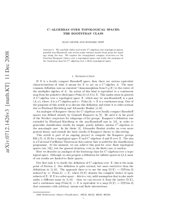
 Ryszard Nest