Systems & Control Letters 20 (1993) 279-288 North-Holland 279 Robust adaptive control of revolute flexible-joint manipulators using sliding technique C h i - M a n K w a n a n d K a i S. Y e u n g Department of Electrical Engineering, The University of Texas at Arlington, Box 19016, Arlington, TX 76019, USA Received 26 April 1992 Revised 7 August 1992 Abstract: In this paper, we present a 3-step procedure to robustly control the revolute flexible-joint manipulator in the presence of parameter variations and bounded input disturbances such as torque ripples. By treating the difference of motor angle and link angle as the input to the rigid link part of the manipulator dynamics, our first step is to design a smooth adaptive reference signal for this input to globally stabilize the rigid subsystem. The second step is to drive the difference of motor and link angles to this desired reference signal exponentially by using sliding control. In the third step we exploit the model reduction capability of sliding control to perform the stability analysis. It is well-known that sliding control can reduce the system order by n if the number of control inputs is n. The exploitation of this property of sliding control makes our stability analysis a lot simpler than other approaches. Global stability in the sense of Lyapunov can be guaranteed and errors in link position and velocity are driven to zero when the system is in sliding mode. No weak elasticity assumption is needed. Keywords: Adaptive control; sliding control; flexible-joint manipulators; Lyapunov function; global stability. 1. Introduction It is quite difficult to control the flexible-joint robot manipulators because the number of degrees of freedom is larger than the number of control inputs. There are several existing approaches to control the system. The integral manifold approach [11] restricts the flexible-joint dynamics to lie on a suitable integral manifold in state space. Only link position and velocity are required for implementation. The demerit is the lack of robustness to parameter variations. Another approach is the feedback linearization method 1-10] which uses nonlinear state transformations to convert the system to the Brunovsky form. This method, however, requires link position, velocity, acceleration and jerk for implementation and is not robust to parameter variations. The third class of controllers is the adaptive control approach. Spong 1,12] combined the globally stable adaptive control law of Slotine and Li 1,8] for the rigid manipulators with an additional correction damping term. Singular perturbation arguments were used to discuss the stability of the closed-loop system. It has been pointed out by Ghorbel et al. 1,3] that the global convergence of the rigid link adaptive control law and the global stability of the boundary layer do not guarantee the stability of the closed-loop flexible-joint system. Several instability mechanisms may destroy the system if some cautions have not been taken into account. Another disadvantage is that only the weak elasticity case has been considered. Chen and Fu 1,1] also attempts to solve the motion control of the flexible-joint system by using adaptive control. Their result is a local result even in the absence of parameter uncertainties. Recently Lozano et al. 1,5] presented a globally stable adaptive control law without using acceleration measurement for the revolute flexible-joint manipulators. Correspondence to." C.-M. Kwan, Department of Electrical Engineering, The University of Texas at Arlington, Box 19016, Arlington, TX 76019, USA. 0167-6911/93/$06.00 © 1993 - Elsevier Science Publishers B.V. All rights reserved 280 C.-M. Kwan, K.S. Yeuny Robust adaptive ~ontrol O[ flexible.:joint manipulator.s In this paper we present a robust adaptive-sliding control law for the revolute flexible-joint manipulator. By treating the difference of motor angle and link angle as the input to the rigid link part of the manipulator dynamics, our first step is to design a smooth adaptive reference signal for this input to globally stabilize the rigid subsystem. The second step is to drive the difference of motor and link angles to this desired reference signal exponentially by using sliding control. In the third step we exploit the model reduction capability of sliding control to perform the stability analysis. It is well-known that sliding control can reduce the system order by n if the number of control inputs is n. The exploitation of this property of sliding control makes our stability analysis a lot simpler than other approaches [1, 4, 5]. Moreover, the external disturbances such as torque ripples can be suppressed easily. In addition, weak joint elasticity is not needed. Global stability in the sense of Lyapunov can be guaranteed and errors in link position and velocity are driven to zero when the system is in sliding mode. The main advantage of this approach is that we can break up the analysis of a complicated problem into several tractable steps. This renders both the analysis and design of complicated systems much simpler and easier. Our paper is organized as follows. Sectio~a 2 describes the design procedure of our approach. The study will be divided into three cases with increasing complexity. A simple one-link example will be given in Section 3 to illustrate our design procedure and performance. Finally some concluding remarks will be included in Section 4. 2. Design procedure The revolute flexible-joint manipulator model [10] can be described as follows: D(ql)¢l + C ( q l , ¢ X ) ¢ l + G ( q l ) = K ( q 2 - ql), (2.1) Jq2 - K ( q l (2.2) - q2) = u + D(ql ) is in R" x, and is known as the inertia matrix. C01 is a vector in R" of the Coriolis and centripetal terms. G is the gravity vector in R". J is the motor inertia matrix in R" ×". ql, 01, ¢1, q2, q2 are vectors in R" which denote the link angles, velocities, accelerations, motor angles, velocities, respectively. K is the joint stiffness matrix in R" ×" which is assumed to be diagonal, d is a vector in R" of bounded external disturbances such as torque ripples, u is a vector in R" of motor torques. The following properties of the rigid part of the manipulator (2.1) are well known in the robotics literature [8, 12]. Property 1: D(ql) is symmetric and positive definite. Property 2." 10(q1) - 2C(ql, ¢1) is skew-symmetric for a suitable representation C(ql, 01). Property 3." (2.1) is linear parametrizable (LP), i.e. /)(ql)¢1 + C(ql, ¢1)01 q- G(ql) = Y(ql, ¢1, ¢1) ~9 where Y is a matrix of known functions, oq~R' is the vector of unknown parameters. We need the following general assumptions throughout the paper: Assumption 1: The bounds of the unknown parameters are known a priori. Assumption 2: qld, the desired trajectory of ql, is continuously differentiable and bounded up to including the fourth order. Assumption 3." ql, 01, ¢1, q2, ¢2 are measurable. Throughout this paper, we shall define q2 - ql in (2.1) as z. Our algorithm can be divided into 3 steps. first step is to find an adaptive reference signal zd which can globally stabilize (2.1) and drive the errors in position and velocity to zero. The second step is to realize the signal Zd by driving z to Zd exponentially. third step is to perform a closed-loop stability analysis when the system is in sliding mode. and The link The C.-M. Kwan, K.S. Yeung / Robust adaptive control of flexible-joint manipulators 281 We divide our studies into the following three cases with increasing complexity: Case 1: Parameters are unknown except for the stiffness matrix K. Case 2: All parameters including K = k ! are unknown. Case 3: All parameters are unknown. K is any diagonal joint stiffness matrix. 2.1. Parameters are unknown except f o r the stiffness matrix K Step 1. Determination of an adaptive reference signal Zd which can globally stabilize (2.1). Using the same notations as in [12], we choose Zd = g-1(19a + Cv + G - (2.3a) gDr) where/), C and t~ represent the corresponding terms D, C and G in (2.1) with estimated parameter values, KD is a known positive definite diagonal matrix, and el = ql -- qld, lY= #ld -- A e l , r = #1 -- v = el + A e l , a = 6. A is a positive definite diagonal matrix and is also a design parameter. Replacing z in (2.1) by Zd in (2.3a) yields D~ + Cr + KDr = Da + Cv + G = Y ( q l , # l , v, a) where 6=fi-O, C, iT= t -G, With the Lyapunov function candidate [12] V = ½ rtOr + ½ el Pc, + ½ g ' r ~ and the adaptation law (2.3b) ,9 = - F - 1 yt r where P and F are symmetric and positive definite constant matrices. It can be easily shown [12] that (2.1) is globally stable in the sense of Lyapunov and e~ and ~ converge to zero. Step 2. Realization of the reference signal Zd (2.3a). After determining the form of Zd, we need to find a way to realize it. If we define r / = z - Zd, Z = q2 -- q~, then our objective in this step is to drive r/to zero. We define the sliding variable as a = ~ + ~q (2.4) where • = diag { ~bx, ~b2. . . . . ~b,} is a positive definite matrix which determines the rate of convergence of q. The reason for the sliding variable definition (2.4) is because, once the system is in sliding, a is confined to zero and q will decay to zero exponentially. Hence, z is driven to Zd exponentially. Note a involves Zd which contains the link acceleration, ~ . Since we do not know parameters exactly, we cannot substitute ql from dynamical equation (2.1). Therefore, we need Assumption 3 of the availability of ~ so that tr is synthesizable. Differentiating a yields (2.5) 6" =/~ + ¢ , f / = f + J - l(u - Kz + d) where f i s a function of q~, 41, q~, q2, #2 and derivatives of the desired trajectory q~d. (2.5) can be expressed as (2.6) 6 = f o + A f + (Jo + AJ)-~(u - Kz + d). Jo and fo are the nominal values of J and f, respectively. Following Assumption 1, the bounds of unknown parameters in D, C, G, J, K are known. A f c a n be shown to be boundable by known functions. Suppose I(Af)~l < Fi, I(J-Xd)~] < Li, I(JolAJ(l+ where F~, L~ and M~j are known functions. J o l A J))~jl < Mij, 282 C.-M. Kwan, K.S. Yeuny. Robust adaptive control (if flexible:joint manipulators From standard results [9] the control law is chosen as (2.7) u = Jo[ - ] o - k~sgn(a)] + K z where -kslsgn(°l)l, k~sgn(a) = k~,sgn(G) .] sgn(.) is the signum function which equals 1 if ( . ) > 0 , according to (l-Mii)k~i>_Fi+Li+ ~ Mi;[(fo)jl+ ~ j=1 0 i f ( o ) = 0 , and - 1 if ( . ) < 0 . k~ is chosen Mijksj+ei, e l > O , i = 1,2 . . . . . n. j=~ i This control law guarantees the following reaching condition for sliding mode: ai6"i < - e i l a ~ ] , i = 1, 2. . . . . n. Hence a goes to zero in finite time, i.e. q tends to zero exponentially. ~ determines the reaching time to sliding. Thus the adaptive reference signal (2.3a) is realized exponentially. Step 3. Stability analysis when system is in sliding mode. The system in sliding is described by Di" + Cr + Kor = Y ~ + Krl, (2.8a) 0 + 4~r/= 0, (2.8b) el + Ael = r. (2.8c) Note that q is an exponentially decaying function. It is a standard practice to neglect the term Kr/in (2.8a) in adaptive control (see p. 213 of [6] and the arguments therein). Consider the following Lyapunov function candidate: 1 t V = ½rtDr + ~eIPel + ½,gtF,9 (2.9a) where P, F are positive definite and symmetric constant matrices. Differentiating (2.9a) along the trajectory of (2.8) and replacing P by 2AtKI:, yields I) = rtDr + ½rtlOr + e~Pdl + ~ t / - ~ = _ ~Kndl _ e~AtKl)Ael <_ O. (2.9b) This shows V, r, et, ~ = r - A e l , and ~ are bounded, which in turn implies i~1 is bounded following Assumption 2 and using (2.1). Thus we see that e~, dl are uniformly continuous as a result of the boundedness of bl, bt. To show el, d~ go to zero as t ~ oo, we need to show in addition that e~, bl are square integrable. Defining y = [e~ b~]t and integrating both sides of (2.9b) from t = 0 to t = ~ , we get V(oo) - V(O) = - y t H y dt (2.10) where H = diag{AtKDA, KD}. From the boundedness of V(t), we conclude that the term on the right-hand side of (2.10) is also bounded which implies that y is square integrable. This together with the uniform continuity and boundedness of ei and ~ imply e~, ~ tend to zero as t ~ oe [6]. The boundedness of q2, q2 follows from (2.8b). Also zd, ~a are bounded because they are functions of bounded quantities el, ~ , and i~. Rem~,rk 1. When all parameters are exactly known (,,Q= 0), there is no need of adaptation and I2 is negative definite. This shows that the system is globally asymptotically stable. Furthermore, there is no need of link acceleration measurement because il~ can be obtained from (2.1). C.-M. Kwan, K.S. Yeung / Robust adaptive control of flexible-joint manipulators 283 Remark 2. When the signum functions in (2.7) are replaced by saturation functions, (2.8b) then becomes, following notations of (2.4), /li + ~bir/i = oi(t), lai(t)l < fii, i = 1, 2. . . . . n. (2.11a) 6i's are known as the sliding layer widths. From [9], the bound for rh in (2.1 la) is given by I~(t)l -< e-¢'tlrh(0)l + 6d~bi. For ease of exposition, we set r//(0) to zero. The case of including rh(0) in the development is straightforward. Hence I1~/11= II['h . . . r/,-Itll < II1-1 1 . . . 1-1t6/~bll = x/n6/q9 (2.11b) where 6 = max{6i}, 4' = min{¢~}, i = 1, 2. . . . , n. Kr/represents a bounded noisy input to (2.8a). Using the same Lyapunov function candidate (2.9a) and notations of (2.10) and (2.11b), V now becomes I I = _ ~tt K D ~ 1 - - e ~ A t K o A e l + rtKrl = - y t H y +yt[A l]tKrl -< -- )~m,n(n)l]Yll 2 + 2m,~(K)Px/~6/¢IIYll = - ~.min(n)liY[I ( Ilyll - 2m"~(K)P'c/n6/dP) 2min(n ) where p = III- Z 1 ] ~11. ~. The technique of 'dead zone' I-6-7, 9] can be used in the adaptation law (2.3b) by setting ,9 = 0 when IlY II -< (2m,x(K)Px/~6/c~)/Amin(H). This guarantees that 1/is non-positive outside the 'dead zone' and hence all parameters and e~, ~ ale bounded. The boundedness of a also guarantees the boundedness of ~/and therefore q2, (h are bounded. Note that the size of'dead zone' depends on 6. Therefore the tradeoff between chattering and tracking accuracy is compromised through the sliding layer width. 2.2. All parameters including K = k ! are unknown Step 1. Determination of an adaptive reference signal Zd. Replacing K by kI in (2.1), we obtain D~h + C(h + G = kz. (2.12) Dividing by k on both sides of (2.12) yields 1 [D(ql)ill + C(qt, ql)ql -~ G(q~)] = z. (2.13) This implies the linear parametrizability (Property 3) is still valid by just redefining the vector of unknown parameters to account for the unknown parameter k. It is obvious that Properties 1 and 2 of the rigid subsystem (2.1) are still valid. We then rewrite (2.13) as Dill + Cql + G = z where D, (7, G denote D/k, C/k and G/k, respectively. Then we choose Zd of the form Zd = Ba + ~V + ~ -- KDr. (2.14a) The notations in (2.14a) have similar meanings as those in (2.3a). Substituting (2.14a) into (2.12) and using the same procedure as in Section 2.1, we obtain the following adaptation law: (2.14b) = -- F - 1 y t r where the following LP property is utilized: + C , + Kor = B a + + = ro All the symbols here have similar meanings as in Section 2.1. Note that Y is still the same as in Section 2.1. Steps 2 and3. The developments in these two parts are exactly analogous to Section 2.1 and hence omitted for brevity. The closed-loop system is globally stable in the sense of Lyapunov and errors in link position and 284 C.-M. Kwan, K.S. Yeung : Robust adaptive control of flexible-joint manipulators velocity converge to zero when system is in sliding. The discussion of using a saturation function is also similar to that of Section 2.1. The design procedure in this subsection will be further illustrated in an example in Section 3 for a 1-1ink robot with strong joint flexibility. 2.3. All parameters are unknown. K is any diagonal joint stifjhess matrix Step 1. Determination of an adaptive reference signal Zd. Multiplying by K-1 on both sides of (2.1) yields D l q l + C l q l + G~ = Z (2.15) where D1, C~ and G~ denote K- 1D, K- 1C and K- ~G, respectively. Though Properties 1 and 2 do not hold in general, equation (2.15) is still LP, i.e. D l q l + C l q I -+ G 1 = Y l ( q l , q l , q l ) L g . We will use Craig's adaptive law [2] to design the reference signal Zd because this approach does not require the skew-symmetry property of (2.15). Zd is then chosen as Zd ---~/)l(qld -- Kvel -- Kpex) + C t q l + G1 (2.16) where Kv, Kp are n x n diagonal positive definite matrices. Substituting (2.16) into (2.15) gives Dlql + Clql + G1 = D1(¢Id-- Kvel -- Kpel) + ~'1 + (~1. (2.17) Adding and subtracting/)~/i on the left-hand side of (2.17) yields 151[~ + Kvi~ + Kpe1] = /)lql + Clql + G1 = (2.18) Y1 ~ where (;)1 = (;)1 - ( ' ) i . The error dynamics is then given by ~ + K~ (2.19) + Kpel = D;1 y ~ (2.19) can be expressed in state-space form: (2.20) fg = A X -'~ BD 1 1 El ~ where A = [ 0 --Kp ' ]' -K~ S = [0], x: Fell Lell' ~ : ~-- tg. Choose the Lyapunov function candidate (2.21) V = ½ x t p x + ½,gtro where P and F are positive definite and symmetric matrices. Taking the derivative of (2.21) along the trajectory of (2.19) yields (2.22) i~ = _ ½ x t Q x + ,~t/-~ + ~ t y ~ l ~ [ 1 B t p x where A t p + P A = - Q, Q = Qt > O. The adaptation law is chosen as O= - F - ~ Y~ Ig~' BtPx. ^ (2.23) It should be noted that parameter projection is needed to ensure the invertibility of D1-t [2]. Substituting (2.23) into (2.22), we get I) = - ½xtQx. (2.24) C.-M. Kwan, K.S. Yeun 9 / Robust adaptive control of flexible-joint manipulators 285 Following a quite similar argument as in Step 3 below (or see Craig [2]), it can be shown that x tends to zero as t--* ~ . Step 2. Realization of zd. Define the sliding variable as a = 0 + ¢,r/ (2.25) where r / = z - zd, z = qz - ql. Following a similar procedure as in Section 2.1, a control law can be chosen to satisfy the sliding condition ai#~ < - e~lail, i = 1, 2 . . . . . n. Step 3. Stability analysis of system in sliding mode. When the system is in sliding mode, the behavior of the system is described by Yc = A x + BD? 1 Y1 ~ + BD? a~l, (2.26a) 0 + q'n = 0. (2.26b) Similar to Step 3 of Case 1, we neglect the effect of t/ because r/ is exponentially decaying. Choose the following Lyapunov function candidate: V = ½ x t p x + ½~tF~ (2.27) Using adaptation law (2.23), it can be shown that (7 = _ ½xt Qx. (2.28) Hence /2 < 0. This implies x e L ~ " , ~ e L L . It follows that zd is bounded, which in turn shows, using Assumption 2 and (2.15) that i~1 is bounded. Hence a~EL~". The boundedness of a~ implies x is uniformly continuous. Now we need to show that x is square integrable. Integrating both sides of (2.28) leads to the conclusion that x is square integrable (see similar arguments as in Step 3 of Section 2.1). Thus x is bounded, uniformly continuous and square integrable. This implies x --+ 0 and t + 00 [6]. The boundedness of q2, q2 can be concluded from the boundedness of r/. Remark 3. The case of using saturation function instead of signum function is completely analogous to the discussion in Section 2.1 and is hence omitted here. 3. Example We consider the same one-link example as in [12]. lgtl + M g L s i n ( q l ) = k(q2 - qt), (3.1a) J?12 - k(ql - q2) = u + d. (3.1b) d is a bounded disturbance which is chosen as 0.5 sin(t)Nm in this example. Defining z = q2 - ql, we then rewrite (3.1a) as I MgL /h + T sin(q1) = z. (3.2) The unknown parameter vector in (3.2) is ,9t = [Ilk, M g L / k ] t. We assume the following values for the parameters in (3.1). The nominal values of I, J, M g L and k are Io = 1 kgm 2, Jo = 1 kgm 2, (MgL)o = 10 Nm, ko = 5 N m / r a d , respectively. The parameter uncertainties in I, J, M g L , k are AI = 0.1 kgm 2, A J = 0.1 kgm 2, A M g L = 5 Nm, Ak = 2.5 Nm/rad, respectively. It should be noted that the stiffness constant k is much smaller than the value of k = 1600 N m / r a d in [12]. This illustrates that our method can handle very flexible manipulators. 286 C.-M. Kwan, K.S. Yeung Robust adaptit;e control of flexible-joint manipulator.s qz O, (tad.) @ l tmae(sec) error in link angle el 0.1~1 <ta°~-a.ml1 \ ~ O i 2 ~ ~ t0 time(see) 9L -O.|U (rad.sec. a) -0.~ O | 0 , 2 4 5 8 LO time(sec) 92 (tad.) time (se~) controlutorque 1 ~ ~ 5 ( i (Nm) O "- 0 | rune(sec) 8 sliding s a b l e it e ,i ~ d lb (sec) Fig. 1. Simulation results of a one-link flexible-joint manipulator. 4. E4. link ~ngle 3. £4. ^ 02 2.t4, el (rad.) (rad.) 1.[4, =I0 2 5. [9 4 5 Ume (sec) time (see) 1. tl~ 4. [9 control torque 2.E8 (Nrn) u (rad.sec. z) time Csee) 5.L14 time (see) Fig. 2. Simulation result of Spong's adaptive controller. C.-M. Kwan, K.S. Yeung / Robust adaptive control of flexible-joint manipulators 287 Our first step is to determine a smooth adaptive reference signal which can stabilize (3.1). Following the procedures in Section 2.2, we can design the following reference signal: (3.3) Zd = ~la + ~2sin(ql) -- kDr where (units are omitted for brevity) qld ---- 1 - - e -t, a : qld F = el -- '~el, ÷ 2el, ko = 10, ,L = 1. The parameter update law is given by ,91 = -- gtar, ,92 = -- g2sin(ql)r, according to (2.14b) gl, g2 are chosen to be 1 and 80 respectively. For the convergence of z to the reference signal Zd, we define r/= z - Zd, Z = q2 variable as a = 0 + ~br/ -- ql, and the sliding (3.4) where ~b is chosen to be 25. Differentiating (3.4) and using (3.1), we get 6 =f+ J-l(u- (3.5) kz + d) where / = ~r) + (~12 + kD) ho = - (glar - ko)el ~ ÷ ~---41COS(q,)--qld]j+ho, gla2(el ÷ t~el) ÷ 2 g l a ( q ~ ) -- ~ l ) r - - ,91qld^ (4) ÷ glarqld(3) ÷ rg2 sin (2ql)41 + (el + ~b~l)g2 sinE(q1 ) - 32 cos (ql)01 ^ ÷ ,9242 sin(q1) ÷ 0.5 g2rsin(2ql)41 + koq~el Following the procedures in Section 2, the control law u is chosen as u = [f~ - ks(t)sat(a/6)] where a=koz + Jo [ - h o - ~ b r l - ( ~ 1 2 +kD) (3)'~1 ToZ~,~,cos(ql)-qld)|, (ko.(MgL)oz ks(t)= ~ 0.5~1(~12 + kD)~l +0.5----)-~o 10, cos(q~)l + 10 +(8-- 1)lal, 1 Jo fl -< Jo + A-------J -< ~ (= 1.1 in this example). The sliding layer width 6 is chosen to be 0.1 radian per second. 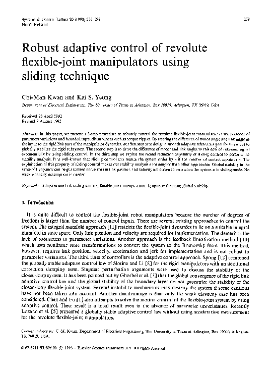All simulations are performed using SIMNON Version 3.1. Simulation results are shown in Figure 1. It is seen that the performance is very good. We have also tried to use Spong's adaptive controller. The system was unstable as shown in Figure 2 because of the strong flexibility k = 7.5 Nm/rad in this example, as compared to k = 1600 Nm/rad in [12]. 4. Conclusion A method of combining sliding and adaptive techniques to control the revolute flexible-joint manipulators is presented. Global stability in the sense of Lyapunov can be guaranteed and errors in link position and 288 C.-M. Kwan, K.S. Yeung / Robust adaptive control qf./texible-joint manipulators velocity are driven to zero when the system is in sliding mode. No assumption of weak elasticity is needed. Our method can also easily suppress input disturbances such as torque ripples. This approach of breaking up a difficult problem into several tractable steps gives a simpler and easier way of analysis and design. The idea here has potential applications in other complicated systems such as the flexible-link manipulators and the force control of multi-link flexible-joint robots. Acknowledgments The authors would like to thank the anonymous reviewers for their many constructive suggestions and comments that lead to a smoother presentation. References [1] K.P. Chen and L.C. Fu, Nonlinear adaptive motion control for a manipulator with flexible joints, in: Proc. IEEE Int. Conj'. Robotics and Automation, 1989. [2] J.J. Craig, Adaptive Control of Mechanical Manipulators (Addison-Wesley, Reading, MA, 1988). [3] F. Ghorbel, J.Y. Hung and M.W. Spong, Adaptive control of flexible joint manipulators, IEEE Control Systems Magazine 9 (1989) 9-13. [4] K.Y. Lian, J.H. Jean and L.C. Fu, Adaptive force control of single-link mechanism with joint flexibility, IEEE Trans. Robotics and Automation 7 (1991) 540-545. [5] R. Lozano and B. Brogliato, Adaptive control of robot manipulators with flexible joints, IEEE Trans. Automat. Contr. 37 (1992) 174 181. [6] K.S. Narendra and A.M. Annaswamy, Stable Adaptive Systems (Prentice-Hall, Englewood Cliffs, N J, 1989). [7] J.E. Slotine and J.A. Coetsee, Adaptive sliding controller synthesis for nonlinear systems, Int. J. Control 48 (1986) PAGES? [8] J.E. Slotine and W. Li, Adaptive manipulator control: A case study, IEEE Trans. Automat. Control 33 (1988) 995-1003. [9] J.E. Slotine and W. Li, Applied Nonlinear Control (Prentice-Hall, Englewood Cliffs, NJ, 1991). [10] M.W. Spong, Modelling and control of elastic joint manipulators. J. Dynam. Systems Measurement Control 109 (1987) 310-319. [11] M.W. Spong, K. Khorasani and P.V. Kokotovic, An integral manifold approach to the feedback control of flexible joints robots, IEEE J. Robotics and Automation 3 (1987) 291-300. [12] M.W. Spong, Adaptive control of flexible joint manipulators, Systems Control Lett. 13 (1989) 15-21.