Title: Southern Ocean carbon sink enhanced by sea-ice feedbacks at the Antarctic Cold Reversal Authors: C.J. Fogwill1,2, C.S.M. Turney2,3,4, L. Menviel2,5, A. Baker2, M. E. Weber6, B. Ellis7, Z.A. Thomas2,3,4, N. R. Golledge8,9, D. Etheridge10, M. Rubino1,10,11, D.P. Thornton10, T.D. van Ommen12,13, A.D. Moy12,13, M.A.J. Curran12,13, S. Davies14, M.I. Bird15,16, N.C. Munksgaard15,17, C.M. Rootes18, H. Millman1,4, J. Vohra2, A. Rivera19,20, A. Mackintosh21, J. Pike22, I.R. Hall22, E.A. Bagshaw22, E. Rainsley1, C. Bronk-Ramsey23, M, Montenari1, A.G. Cage1, M.R.P. Harris1, R. Jones24†, A. Power24, J. Love24, J. Young25, L.S. Weyrich3,25, A. Cooper26 Affiliations: 1School of Geography, Geology and the Environment, Keele University, Staffordshire, UK 2Palaeontology, Geobiology and Earth Archives Research Centre, School of Biological Earth and Environmental Sciences, University of New South Wales, 2052, Australia 3ARC Centre of Excellence in Australian Biodiversity and Heritage, School of Biological Earth and Environmental Sciences, University of New South Wales, 2052, Australia 4Chronos 14Carbon-Cycle 5Climate Facility, University of New South Wales, 2052, Australia Change Research Centre, School of Biological Earth and Environmental Sciences, University of New South Wales, 2052, Australia 6Department of Geochemistry and Petrology, Institute of Geosciences, University of Bonn, Bonn, 53115, Germany 7Research 8Antarctic School of Earth Sciences, Australian National University, Canberra, Australia Research Centre, Victoria University of Wellington, Wellington 6140, New Zealand 9GNS Science, Lower Hutt, 5001, New Zealand 10CSIRO Oceans and Atmosphere, Aspendale, Victoria, 3195 Australia 11Dipartimento di Matematica e Fisica, Università della Campania "Luigi Vanvitelli", viale Lincoln, 5-81100 Caserta, Italy 12Department of Agriculture, Water and the Environment, Australian Antarctic Division, 203 Channel Highway, Kingston, Tasmania 7050, Australia 13Antarctic Climate & Ecosystems Cooperative Research Centre, University of Tasmania, Private Bag 80, Hobart, Tasmania 7001, Australia 14Department 15Centre of Geography, Swansea University, Swansea, United Kingdom for Tropical Environmental and Sustainability Science, College of Science, Technology and Engineering, James Cook University, Cairns, Australia 16ARC Centre of Excellence in Australian Biodiversity and Heritage, James Cook University, Cairns, Australia 17Research Institute for the Environment and Livelihoods, Charles Darwin University, Australia 18Department of Geography, University of Sheffield, United Kingdom 19 Instituto de Conservación, Biodiversidad y Territorio, Universidad Austral de Chile, Chile 20 Departamento de Geografia, Universidad de Chile, Portugal 84, Santiago 8331051, Chile 21School of Earth, Atmosphere and Environment, Monash University, Melbourne, Australia 22School of Earth and Ocean Sciences, University of Cardiff, Wales, UK 23Research Laboratory for Archaeology and the History of Art, University of Oxford, Dyson Perrins Building, South Parks Road, Oxford, OX1 3QY, UK 24BioEconomy Centre, The Henry Wellcome building for Biocatalysis, Biosciences, Stocker Road, Exeter University, Exeter, EX4 4QD, UK 25Australian 26South Centre for Ancient DNA, University of Adelaide, 5005, Australia Australian Museum, Adelaide, South Australia 5005, Australia †Deceased Contact Information: *Correspondence to c.j.fogwill@keele.ac.uk The Southern Ocean occupies some 14% of the planet’s surface and plays a fundamental role in the global carbon cycle and climate. It provides a direct connection to the deep ocean carbon reservoir through biogeochemical processes that include surface primary productivity, remineralisation at depth, and the upwelling of carbonrich water masses. However, the role of these different processes in modulating past and future air-sea carbon flux remains poorly understood. A key period in this regard is the Antarctic Cold Reversal (ACR, 14.6-12.7 kyr BP), when mid- to high-latitude Southern Hemisphere cooling coincided with a sustained plateau in the global deglacial rise in atmospheric CO2. Here we reconstruct high-latitude Southern Ocean surface productivity from marine-derived aerosols captured in a highly-resolved horizontal ice core. Our multiproxy reconstruction reveals a sustained signal of enhanced marine productivity across the ACR. Transient climate modelling indicates this period coincided with maximum seasonal variability in sea-ice extent, implying that sea-ice biological feedbacks enhanced CO2 sequestration and created a significant regional marine carbon sink, which contributed to the plateau in CO2 at the ACR. Our results highlight the role Antarctic sea ice plays in controlling global CO2, and demonstrates the need to incorporate such feedbacks into climate-carbon models. 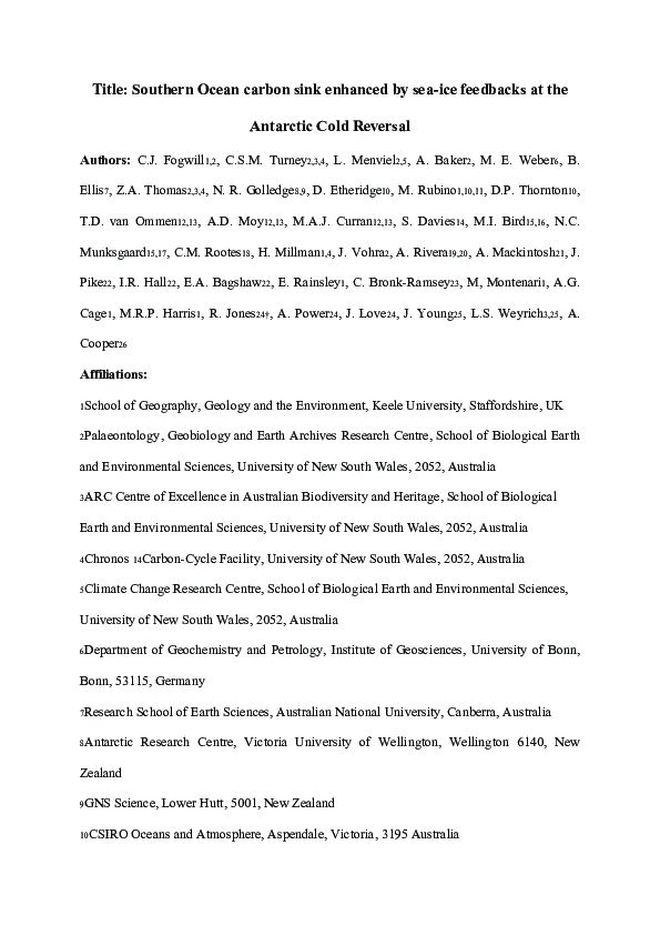The Last Glacial Transition (LGT; 18,000-11,000 years ago or 18-11 kyr BP) experienced rapid and sustained changes in atmospheric CO2 (rising from approximately 190 parts per million (ppm) to around 270 ppm; Figure 1), providing us with the potential to gain valuable insights into climate-carbon dynamics1. Detailed analysis of the stable isotopic composition of atmospheric carbon dioxide (δ13C-CO2)1,2 from Antarctic ice cores suggests terrestrial carbon may have played a substantial role in rapid CO 2 rises, but variability across the LGT may reflect a combination of sources, sinks and feedbacks. Parallel changes in Antarctic temperature and atmospheric CO2 have been interpreted as the Southern Ocean playing a key role in the global carbon budget3-5, but detailed mechanisms remain unresolved. Several physical and biological mechanisms have been invoked to explain these observations, including: changes in the strength and/or latitudinal migration of the mid-latitude jet stream and prevailing surface westerly airflow influencing Southern Ocean overturning4,6-8; variations in iron (dust) fertilisation of subantarctic phytoplankton impacting the biological carbon pump efficiency9-11; sea-ice controlling CO2 exchange12,13 and carbon drawdown14; and the potential impacts of a warming ocean on CO2 exchange1. The role of the Southern Ocean as a source or sink of atmospheric carbon during the LGT remains highly contested, with the above processes not fully accounting for the changes in CO2 recorded over this period9, implying that one or more mechanisms are currently not captured in our understanding15,16. A striking feature of the LGT record is a 1,900 year-long plateau in CO2 concentration, when the ongoing rise in CO2 paused at a near-constant 240 ppm during the Antarctic Cold Reversal (ACR)17, a period characterised by surface cooling across the mid- to high-latitudes of the Southern Hemisphere18-20. The ACR was coincident with sustained warming across the Northern Hemisphere (the North Atlantic Bølling-Allerød interstadial)9,17 and abrupt global sea level rise21,22, as well as major disruptions to atmospheric and ocean circulation8,22 and the carbon cycle (Figure 1)9,10,23. Whilst the global sequence of events during the ACR is reasonably well known19, a clear understanding of the drivers and impacts of contrasting polar climate changes on global CO2 trends has proved elusive, owing to the challenges in precisely aligning ice and marine records across this period9. This reflects the lack of wellresolved, high-accumulation marine sedimentary records from the high-latitude Southern Ocean. One crucial record in this regard comes from marine sediment core TN057-13 (~53°S 5°E)4,9 (Figure 2), which suggests the ACR was characterised by reduced carbon sequestration in the mid to high-latitudes (measured by decreased biological productivity or export production 4,5; Figure 1E). This was possibly the result of enhanced stratification, which decreased the vertical supply of nutrients across the high-nutrient, low-chlorophyll (HNLC) sectors of the Southern Ocean during cooling4. However, such a hypothesis is difficult to test in the absence of a network of well-resolved records of productivity from the high latitudes of the Southern Ocean. Southern Ocean productivity polewards of TN057-13 has been previously recorded in the Scotia Sea from marine core MD07-3134, (~59°S 42°W; Figures 1F and 2; see Supplementary Information)21. In common with core TN057-13, this sequence is exceptionally well-resolved (with sedimentation rates of 20 to 200 cm/kyr21) and, given the location, records changes south of the Polar Front, even during glacial terminations24. After accounting for sediment focussing with 230 Th normalisation (see Supplementary Information)25, MD07-3134 opal burial rates provide estimated changes in biological productivity (export production) (Figure 1F). This suggests that export production in the high-latitude Southern Ocean increased from ~17 ka, in line with that shown to the north in core TN057-13; however, subsequently, export production in the high-latitude Southern Ocean (MD07-3134) continued to increase through the ACR, in antiphase to the trend recorded further north (TN057-13)4 (Figures 1 and 2). This indicates that different driver(s) of marine biological activity may have operated across the high latitudes, contributing to the sustained ACR CO2 plateau. In the absence of a network of highly-resolved marine records from the high-latitude Southern Ocean (that are normalised through 230Th)24, we present a new reconstruction of high-latitude surface ocean productivity from aerosol derived marine biomarkers captured in a highly-resolved horizontal ice core from the Weddell Sea, Antarctica22 that record regionalscale environmental processes operating across the south Atlantic sector of the Southern Ocean during the LGT (Figure 2)22,26. The Patriot Hills blue ice record A new ‘horizontal’ ice core record was developed from the exposed blue ice area (BIA) at the Patriot Hills in Horseshoe Valley, Ellsworth Mountains (Figure 2) 22, where ancient ice has been drawn up to the surface of the ice sheet. With a well-constrained chronology, uninterrupted sequence of ice through the LGT (Figure 3; Methods), and contemporary precipitation and aerosol delivery from the South Atlantic sector of the Southern Ocean (Figure 2; Supplementary Information)27, the Patriot Hills is ideally placed to record environmental changes across the high-latitude South Atlantic. The record provides unrestricted volumes of ice of known age, offering a unique opportunity to develop innovative multiproxy biomarker reconstructions22,28. In contrast to many other BIAs, the site has not been mixed through ice flow, providing a coherent stratigraphic succession across the LGT (Figure 3, Methods and Supplementary Information)22,29. Identifying marine biomarkers in ancient ice To examine regional environmental responses through the LGT, fluorescent organic matter (fOM) analysis and liquid chromatography organic carbon detection (LC-OCD)30 was undertaken across the Patriot Hills record, to identify biomarker signals and quantify changes in dissolved organic carbon (DOC) before and after the ACR (see Figure 4, Methods and Supplementary Information)30. Detailed analysis (using an Aqualog®) of fOM emission spectra from samples taken at depth identified two protein-like components in ice across the profile, TRYLIS and TYLIS: tryptophan and tyrosine-like substances31 (see Methods and Supplementary Information). Whilst there are limited studies of such biomarkers in ancient Antarctic ice32, past work has unambiguously demonstrated that a strong TRYLIS microbial signal is found in contemporary Antarctic snow and ice derived from precipitation and aerosols from the marine environment33-35. Previous work on the West Antarctic Ice Sheet Divide ice core (WAIS Divide) using similar fOM approaches, epifluorescence microscopy and flow cytometry, has identified chlorophyll and tryptophan in ancient ice, demonstrating that these are primarily derived from marine aerosol sources, rather than being solely geomicrobial (in situ) in origin34,35 (Methods and Supplementary Information). These studies have also identified inter-annual variability in the fOM signal, concluding that in situ secondary production or post-depositional alteration of fOM in ice are unlikely to be primary factors in interpreting marine fOM signals in Antarctic ice cores (see Methods and Supplementary Information)34,35. To examine the source of the fOM signal in the Patriot Hills BIA, and test our hypothesis of a marine origin35 we applied imaging flow cytometry (IFC; ImageStream®) and Scanning Electron Microscopy (SEM) to the Patriot Hills samples to identify microscopic populations within the ice (Figure 4, see Methods and Supplementary Information). IFC on samples across the record reveals four significant non in-situ microbial populations (Figure 4C) based on the autofluorescence and morphology of particulates: nanoplankton36; eukaryotic picoplankton37; chitin37; and crypto-tephra and/or wind-blown dust22. SEM analysis on unvortexed samples demonstrates that the eukaryotic picoplankton and the chitin populations are related (Figure 4D). These marine populations are represented in all samples analysed throughout the profile, and whilst IFC is not quantitative it provides valuable independent support for the fOM signal being marine in origin. Together, the fOM, LC-OCD and IFC analysis indicate that marine biomarkers are present throughout the profile, in agreement with other Antarctic ice core studies34,35. Intercomparison of biomarkers from the Patriot Hills BIA In comparing the records of fOM across the LGT we observe a pronounced intensity peak related to autofluorescence of marine biomarkers across the ACR section of the Patriot Hills BIA (Figure 4A and 5F). This change in fOM signal could reflect marked changes in precipitation source over the LGT; however, we discount this through regime shift analysis38 on the deuterium-excess profile, which reveals no significant variability across the ACR or the LGT, at either 99% or 95% confidence, indicating that the precipitation source remained constant over the LGT (Figure 3B). This implies that the intensity of the fOM signal reflects an increase in the autofluorescent marine biomarkers in the precipitation and aerosol source regions, associated with nanoplankton, picoplankton and picoeukaryotes as identified through IFC. We focus on the variation in the TRYLIS fOM component, which represents 83.33% of the variance in fOM signal (Methods and Supplementary Information). The TRYLIS component is highly variable across the BIA record, but has a sustained high concentration across the period defined by the ACR (Figures 4 and 5). This pattern is mirrored in samples taken from a parallel transect from the Patriot Hills BIA, demonstrating the robustness of the fOM signal (Extended Data). To further investigate the detail of the marine biomarker signals, large-volume ice samples were taken across key transitions of the Patriot Hills BIA to extract ancient bacterial DNA in situ by directly melting and filtering ice from specific time-horizons –maximising the signal and minimising contamination (Figure 4B, Methods and Supplementary Information) – allowing the identification of picoplankton, picoeukaryotes and nanoplankton at a taxa level. 16S rRNA indexing reveals that a marked ecological switch – characterised by the appearance of an exceptionally diverse range of halotolerant microorganisms commonly found in seawater – was observed during the ACR, coincident with the increase in fOM TRYLIS signal (Figure 4B). Specifically, we found that the marine-associated taxa Salinibacterium, (f) Erythrobacteraceae, Rhodobacteraceae, Marinobacter and Pseudidiomarina are statistically associated with the ACR period (p<0.038). The increase in species diversity (predominantly marine taxa) compared to that observed during either the mid-Holocene or Last Glacial Maximum is marked (Figures 4 and 5). Whilst the source of this signal could have been from brine pools associated with sea-ice build-up, the signal likely reflects an enhanced diversity and productivity from an open marine, or marginal seaice zone, an interpretation that agrees with the WAIS divide ice core analysis34,35. With four independent approaches (LC-OCD, IFC analysis, fOM and DNA) providing a record of marine biological productivity in the high-latitude South Atlantic sector of the Southern Ocean, our results strongly suggest that the ACR was a period of enhanced marine biological productivity and diversity. With the enhanced picoplankton and picoeukaryotes signals derived from the surface precipitation and aerosol source waters of the HNLC Southern Ocean during the ACR, we suggest that there was sustained strengthening of the biological pump, similar to the effects of contemporary iron fertilisation experiments16, a finding that supports the enhanced export production recorded in marine sediments from the Scotia Sea (Figure 1F)21. Comparison between marine and terrestrial records To reconcile the apparent conflict between the increase in marine productivity across the ACR recorded in marine cores from the Scotia Sea (MD07-3134) and the Patriot Hills BIA with the decrease reported further north in the South Atlantic (TN057-13)4,9 (Figure 1), we compare our record of marine biomarkers (fOM) captured in the Patriot Hills ice with potential drivers of Southern Ocean productivity: iceberg rafted debris (IBRD; a proxy for Antarctic iceberg discharge)21, sea salt sodium (ssNa+) from the EDML ice core (a proxy for sea-ice extent)39, and proxy sea-ice reconstructions40,41. We further compare these records to published independent transient modelling experiments using LOVECLIM, which include fresh water hosing in the Ross and Weddell Seas42 (Figure 5; Supplementary Information). During the LGT, these comparisons indicate weak relationships between inferred marine biological productivity, sea-ice expansion, atmospheric CO2 variability and the peak in marine derived biomarkers (fOM) between ~24 and ~14.6 kyr BP, agreeing with previous studies (Figure 5)43. This contrasts with the period defined by the ACR, where we observe a strong relationship between marine fOM in the Patriot Hills BIA, increased production of biogenic opal in the Scotia Sea, and the extended atmospheric CO 2 plateau (Figures 1 and 5). Given that this increase in marine productivity seen in the Scotia Sea during the ACR is not apparent in mid-latitude marine records (Figure 2)4,9, we focus on possible high-latitude drivers of CO2 exchange: iron fertilisation from enhanced IBRD flux44; a reduction in Antarctic Bottom Water (AABW) formation due to enhanced freshwater flux 45-47; and sea-ice feedbacks40. IBRD contains high concentrations of bioavailable iron, making iceberg melt a potential source for increased primary productivity and carbon sequestration through fertilisation across the HNLC regions of the high-latitude Southern Ocean44. However, despite significant evidence for potential enhanced iron fertilisation of the Southern Ocean through increased delivery of IBRD at around 20-19 kyr BP and 17-16 kyr BP21, there does not appear to be a strong biological response in the Patriot Hills fOM or Scotia Sea opal flux records (Figures 2 and 5), suggesting enhanced IRBD influx did not lead to increased high-latitude marine export production. Another possibility is ice-sheet drawdown across the Weddell Sea Embayment21,22, with associated meltwater influx that may have triggered stratification and substantial circulation changes across the broader Southern Ocean, magnified by associated shifts in the intensity and/or location of surface westerly air flow4,9,22,48; this is supported by independent ice-sheet and Earth system modelling experiments21,42. However, the disparity in the opal flux records between marine cores from the mid-latitude South Atlantic4 and Scotia Sea argues that the enhanced ACR export production was focussed on the high-latitude South Atlantic across the Scotia Sea (Figure 1). An alternative mechanism involves sea-ice feedbacks, which have been implicated in amplifying climate and ice sheet feedbacks across the ACR 19,46. Recent studies of full glacial conditions suggest that reduced surface–deep ocean exchange and enhanced micro nutrient consumption by phytoplankton in the Southern Ocean may have lowered atmospheric CO240,43. During the austral winter, sea-ice expansion allowed the mixed layer to deepen, ‘refuelling’ the surface ocean with micro nutrients from the deep ocean reservoir, and enhancing near-surface productivity and export production during the breakup of sea ice in the subsequent summer. This was likely amplified by the addition of iron from sea-ice melt and breakup in the post-glacial HNLC ocean, and possibly also by seasonal temperature changes and CaCO3 dissolution13. Proxy records and the LOVECLIM transient Earth system modelling42 suggest the highest seasonal variability in sea-ice extent across the LGT took place during the ACR (with greatest extent during winter and spring) (Figure 5), implying that sea-ice feedbacks were amplified across this period (Figure 6). These conditions contrast markedly with the periods immediately prior to (Figure 6A) and following (Figure 6D) the ACR, when the seasonal sea ice zone was relatively less variable (Figure 5), the high-latitude Southern Ocean less stratified21,42,46, and the locations of the Intertropical Convergence Zone (ITCZ) and mid-latitude Southern Hemisphere Westerlies were relatively south (Figure 2). Set against a backdrop of a warming ocean during the LGT, these conditions likely created ideal conditions for enhanced Southern Ocean productivity in the high-latitude Southern Ocean, especially in sectors of the South Atlantic such as the Weddell and Scotia Seas. Comparison between our continuous Scotia Sea opal flux record 21 and the Patriot Hills BIA fOM record indicates the high-latitude signal of enhanced surface marine primary productivity was related to marked seasonal sea-ice variability during the ACR, a period characterised by a sustained atmospheric CO 2 plateau9,17,23. During the ACR, most marine records across the mid-latitudes suggest the biological pump in the Southern Ocean weakened, in apparent contradiction of the plateau in atmospheric CO 2 at that time (Figure 1). Our results indicate that despite low dust input (Figure 1) and surface cooling across subantarctic waters during the ACR, marked variability in sea-ice extent resulted in increased seasonal surface productivity in the HNLC waters of the high-latitude South Atlantic sector of the Southern Ocean, in comparison to periods prior to and following this event (Figure 5). We suggest that increased seasonal marine primary productivity in fact enhanced the Southern Ocean organic carbon pump, increasing carbon drawdown and leading to enhanced export production (Figure 6). Whilst other mechanisms may have played a part in the ACR CO2 plateau – including iron fertilisation, cool Southern Ocean surface temperatures and possibly reductions in the rate of AABW formation8 – our observation that seasonal Southern Ocean sea-ice feedbacks in the South Atlantic sector of the high-latitude Southern Ocean may have contributed to a slowdown in the rate of CO 2 rise during the ACR has significant implications for our understanding of the role of the Southern Ocean in global carbon dynamics. Our results imply that during periods of Southern Ocean sea-ice expansion, high variability in winter and summer sea-ice extent may result in enhanced carbon sequestration – as seen recently with significant sea ice variability enhancing benthic carbon drawdown14 – providing a negative feedback during periods of rising CO2. This finding has ramifications for our understanding of contemporary ice-ocean-carbon feedbacks, and confirms the dynamic role Antarctic sea ice plays in providing a negative feedback during periods of rising CO2. This mechanism requires detailed modelling assessment with high-resolution tracer enabled models that capture such processes 49, particularly given recent Antarctic sea ice changes50, which may impact the efficiency of the Southern Ocean as carbon sink in the future14. Figure Captions Figure 1. Intercomparison of Antarctic ice core with marine proxy records from independent referenced studies. a. WAIS divide core (WDC51) δ18O isotopic record. b. CO2 concentration from WDC (WD2014 chronology)17 c. Cariaco Basin grey scale (measure of latitudinal changes in the trade winds related to the Intertropical Convergence Zone (ITCZ)48). d. nonsea salt Ca2+ (nssCa2+) from EPICA Dronning Maud Land (EDML)52. E. South Atlantic opal flux from TN057-13 (blue)4. F. Scotia Sea opal flux core MD07-3134 (red)21. Vertical boxes indicate the periods defined by the Antarctic Cold Reversal (ACR) (blue), the Younger Dryas (YD) chronozone (pink; 11.7-12.7 kyr BP). Figure 2. The South Atlantic sector of the Southern Ocean with the locations of Patriot Hills in the Ellsworth Mountains, the EPICA Dronning Maud Land (EDML) ice core52, and marine cores MD07-313421 and TN057-134. Positions of the southern limb of the Antarctic Circumpolar Current (purple line), the polar front (red), subantarctic front (green) and the subtropical front (yellow)53. Inset. Monthly grouped 72-hour atmospheric back trajectories for the Patriot Hills (November 2009), from the NOAA HySPLIT54, with WAIS Divide (WDC) and EDML ice cores. South Pole Stereographic basemap produced in Generic Mapping Tools v5.4.5 (ref55) with the NOAA ETOPO1 Ice Surface dataset. Figure 3. Stratigraphic and chronological details of the Patriot Hill Blue ice area (BIA). a. Schematic stratigraphic succession from Ground Penetrating Radar (GPR), across the Patriot Hills BIA, indicating ice accumulation punctuated by two periods of erosion (D1 and D2; thick black lines), and the position of known tephras (red lines)22. b. d-excess across profile; solid horizontal black lines denote potential regime shifts at 99% confidence, dashed black lines denote potential regime shifts at 95% confidence38. c. Age-depth model between D1 ~21 ka (21,000 years) and D2 ~10 ka (10,000 years) with volcanic ‘tephra’ horizons (TD822a and WCM-93-25) marked (see Supplementary Information22). Figure 4. Marine biomarkers from Patriot Hills blue ice area (BIA). a. 5m resolved fOM intensity. b. Percentage marine taxa from 16S rRNA extractions (top Powerlyzer, middle CTAB), and (Lower) LC-OCD component analysis with dissolved organic carbon (DOC; ppb). LGT and ACR periods highlighted in grey and blue respectfully. c. Marine populations from IFC (ImageSteam®) (sample 380 m), i) Nanoplankton, ii) Eukaryotic picoplankton, iii) Chitin, and iv) non-fluorescent dust (left to right: brightfield (Ch01), autofluorescence (Ch02) and side scatter (Ch06)). Sub-populations differentiated based on Intensity vs Aspect ratio (central plot). d. SEM of picoeukaryotes with chitin (tails) at 7,000 and 16,000 magnification. Figure 5. Regional climate proxy and model intercomparisons with the Patriot Hills record. a. Diatom transfer function-based winter sea-ice concentration41. b. Sea salt (ssNa+) from EPICA Dronning Maud Land (EDML)52. c. Iceberg-rafted debris flux (IBRD) from MD07313421 (normalised 100-year, relative to Holocene). d. Modelled seasonal difference in Antarctic sea-ice area (LOVECLIM42). e. Percentage marine microorganisms from 16S rRNA CTAB extraction (upper), and Powerlyzer (Lower). f. fOM concentration (Component 1; TRYLIS). Vertical boxes indicate the Antarctic Cold Reversal (ACR) (blue), and Younger Dryas (YD) chronozones (11.7-12.7 ka). Black triangles represent the age tie points. Figure 6. Schematic depicting events across mid to high-latitude Southern Ocean during the Last Glacial Transition. a. Post-Last Glacial Maximum (LGM). Displacement of the Southern Hemisphere Westerlies (SHW), enhances overturning of mid-latitude Southern Ocean between ~17 ka- 14.7 ka evidenced by opal flux4. b. Antarctic Cold Reversal (ACR). Enhanced intrusion of Circumpolar Deepwater (CDW) and winter sea-ice (WSI) expansion (winter / spring winter). Increased stratification, mixed layer deepening and reduction in Antarctic Bottom Water (AABW)40. c. ACR (summer/autumn), WSI break up enhances CO2 drawdown at high latitudes. d. Younger Dryas chronozone, reinvigorated mid-latitude overturning and degassing of old CO2 enhancing opal flux. References 1 2 3 4 Bauska, T. K. et al. Carbon isotopes characterize rapid changes in atmospheric carbon dioxide during the last deglaciation. Proceedings of the National Academy of Sciences 113, 3465-3470, (2016). Bauska, T. K. et al. Controls on millennial‐scale atmospheric CO2 variability during the last glacial period. Geophysical Research Letters 45, 7731-7740 (2018). Monnin, E. et al. Atmospheric CO2 Concentrations over the Last Glacial Termination. Science 291, 112-114, (2001). Anderson, R. F. et al. Wind-Driven Upwelling in the Southern Ocean and the Deglacial Rise in Atmospheric CO2. Science 323, 1443-1448, (2009). 5 6 7 8 9 10 11 12 13 14 15 16 17 18 19 20 21 22 23 24 25 Gottschalk, J. et al. Biological and physical controls in the Southern Ocean on past millennial-scale atmospheric CO2 changes. Nature Communications 7, 11539. (2016). Toggweiler, J. R., Russell, J. L. & Carson, S. R. Midlatitude westerlies, atmospheric CO2, and climate change during the ice ages. Paleoceanography 21(2) (2006). Marshall, J. & Speer, K. Closure of the meridional overturning circulation through Southern Ocean upwelling. Nature Geoscience 5, 171-180 (2012). Huang, H., Gutjahr, M., Eisenhauer, A. & Kuhn, G. No detectable Weddell Sea Antarctic Bottom Water export during the Last and Penultimate Glacial Maximum. Nature Communications 11, 424, 14302 (2020). Jaccard, S. L., Galbraith, E. D., Martínez-García, A. & Anderson, R. F. Covariation of deep Southern Ocean oxygenation and atmospheric CO2 through the last ice age. Nature 530, 207-210, (2016). Martínez-García, A. et al. Iron Fertilization of the Subantarctic Ocean During the Last Ice Age. Science 343, 1347-1350, (2014). Jaccard, S. L. et al. Two Modes of Change in Southern Ocean Productivity Over the Past Million Years. Science 339, 1419-1423, (2013). Butterworth, B. J. & Miller, S. D. Air-sea exchange of carbon dioxide in the Southern Ocean and Antarctic marginal ice zone. Geophysical Research Letters 43, 7223-7230. (2016). Delille, B. et al. Southern Ocean CO2 sink: The contribution of the sea ice. Journal of Geophysical Research: Oceans 119, 6340-6355, (2014). Barnes, D. K. A. Antarctic sea ice losses drive gains in benthic carbon drawdown. Current Biology 25, (2015). Boyd, P. W., Claustre, H., Levy, M., Siegel, D. A. & Weber, T. Multi-faceted particle pumps drive carbon sequestration in the ocean. Nature 568, 327-335, (2019). Boyd, P. W. et al. A mesoscale phytoplankton bloom in the polar Southern Ocean stimulated by iron fertilization. Nature 407, 695, (2000). Marcott, S. A. et al. Centennial-scale changes in the global carbon cycle during the last deglaciation. Nature 514, 616-619, (2014). Fogwill, C. J. & Kubik, P. W. A glacial stage spanning the Antarctic Cold Reversal in Torres del Paine (51 degrees S), Chile, based on preliminary cosmogenic exposure ages. Geografiska Annaler Series a-Physical Geography 87A, 403-408 (2005). Pedro, J. B. et al. The spatial extent and dynamics of the Antarctic Cold Reversal. Nature Geosci 9, 51-55. (2015). McGlone, M. S., Turney, C. S. M., Wilmshurst, J. M., Renwick, J. & Pahnke, K. Divergent trends in land and ocean temperature in the Southern Ocean over the past 18,000 years. Nature Geoscience 3, 622-626, (2010). Weber, M. E. et al. Millennial-scale variability in Antarctic ice-sheet discharge during the last deglaciation. Nature 510, 134-138, doi:10.1038/nature13397 (2014). Fogwill, C. et al. Antarctic ice sheet discharge driven by atmosphere-ocean feedbacks at the Last Glacial Termination. Scientific reports 7, 39979 (2017). Schmitt, J. et al. Carbon Isotope Constraints on the Deglacial CO2 Rise from Ice Cores. Science 336, 711-714, 1217161 (2012). Sprenk, D. et al. Southern Ocean bioproductivity during the last glacial cycle – new decadal-scale insight from the Scotia Sea. Geological Society, London, Special Publications 381, 245-261, (2013). Meyer-Jacob, C. et al. Independent measurement of biogenic silica in sediments by FTIR spectroscopy and PLS regression. Journal of Paleolimnology 52, 245-255, (2014). 26 27 28 29 30 31 32 33 34 35 36 37 38 39 40 41 42 43 44 Turney, C. S. M. et al. Late Pleistocene and early Holocene change in the Weddell Sea: a new climate record from the Patriot Hills, Ellsworth Mountains, West Antarctica. Journal of Quaternary Science 28, 697-704 (2013). Tetzner, D., Thomas, E. & Allen, C. A. Validation of ERA5 Reanalysis Data in the Southern Antarctic Peninsula—Ellsworth Land Region, and Its Implications for Ice Core Studies. Geosciences 9. 7. 289 (2019). Turney, C. S. M. et al. Early Last Interglacial ocean warming drove substantial ice mass loss from Antarctica. Proceedings of the National Academy of Sciences 117, 3996-4006, (2020). Winter, K. et al. Assessing the continuity of the blue ice climate record at Patriot Hills, Horseshoe Valley, West Antarctica. Geophysical Research Letters 43, 20192026 (2016). Huber, S. A., Balz, A., Abert, M. & Pronk, W. Characterisation of aquatic humic and non-humic matter with size-exclusion chromatography – organic carbon detection – organic nitrogen detection (LC-OCD-OND). Water Research 45, 879-885, (2011). Jørgensen, L. et al. Global trends in the fluorescence characteristics and distribution of marine dissolved organic matter. Marine Chemistry 126, 139-148 (2011). D'Andrilli, J., Foreman, C. M., Sigl, M., Priscu, J. C. & McConnell, J. R. A 21,000 year record of organic matter quality in the WAIS Divide ice core. Clim. Past Discuss. 2016, 1-15, (2016). Smith, H. J. et al. Microbial formation of labile organic carbon in Antarctic glacial environments. Nature Geosci 10, 356-359, (2017). Rohde, R. A., Price, P. B., Bay, R. C. & Bramall, N. E. In situ microbial metabolism as a cause of gas anomalies in ice. Proceedings of the National Academy of Sciences 105, 8667-8672, (2008). Price, P. & Bay, R. Marine bacteria in deep Arctic and Antarctic ice cores: a proxy for evolution in oceans over 300 million generations. Biogeosciences 9, 3799-3815 (2012). Moorthi, S., Caron, D., Gast, R. & Sanders, R. Mixotrophy: a widespread and important ecological strategy for planktonic and sea-ice nanoflagellates in the Ross Sea, Antarctica. Aquat Microb Ecol 54, 269-277 (2009). Massana, R. Eukaryotic picoplankton in surface oceans. Annual review of microbiology 65, 91-110 (2011). Rodionov, S. N. A sequential algorithm for testing climate regime shifts. Geophys. Research Letters 31 (2004). Wolff, E. W. et al. Southern Ocean sea-ice extent, productivity and iron flux over the past eight glacial cycles. Nature 440, 491-496, (2006). Abelmann, A. et al. The seasonal sea-ice zone in the glacial Southern Ocean as a carbon sink. Nature Communications 6, 8136, (2015). Esper, O. & Gersonde, R. New tools for the reconstruction of Pleistocene Antarctic sea ice. Palaeogeography, Palaeoclimatology, Palaeoecology 399, 260-283, (2014). Menviel, L., A. Timmermann, O. Elison Timm & Mouchet, A. Deconstructing the Last Glacial Termination: the role of millennial and orbital-scale forcings. Quaternary Science Reviews 30, 1155-1172 (2011). Collins, L. G., Pike, J., Allen, C. S. & Hodgson, D. A. High-resolution reconstruction of southwest Atlantic sea-ice and its role in the carbon cycle during marine isotope stages 3 and 2. Paleoceanography 27 (3) (2012). Duprat, L. P. A. M., Bigg, G. R. & Wilton, D. J. Enhanced Southern Ocean marine productivity due to fertilization by giant icebergs. Nature Geoscience 9, 219-221, (2016). 45 46 47 48 49 50 51 52 53 54 55 Fogwill, C. J., Phipps, S. J., Turney, C. S. M. & Golledge, N. R. Sensitivity of the Southern Ocean to enhanced regional Antarctic ice sheet meltwater input. Earth's Future 3, 317-329, (2015). Golledge, N. R. et al. Antarctic contribution to meltwater pulse 1A from reduced Southern Ocean overturning. Nature Communication 5, 6107 (2014). Menviel, L., Timmermann, A., Timm, O. E. & Mouchet, A. Climate and biogeochemical response to a rapid melting of the West Antarctic Ice Sheet during interglacials and implications for future climate. Paleoceanography 25, (2010). Hogg, A. et al. Punctuated shutdown of Atlantic Meridional Overturning Circulation during the Greenland Stadial 1. Scientific Reports 6 (2016). Menviel, L. et al. Southern Hemisphere westerlies as a driver of the early deglacial atmospheric CO2 rise. Nature Communications 9, 2503, (2018). Parkinson, C. L. A 40-y record reveals gradual Antarctic sea ice increases followed by decreases at rates far exceeding the rates seen in the Arctic. Proceedings of the National Academy of Sciences 116, 29, 14414-14423. (2019). WAIS Divide Members. Precise interpolar phasing of abrupt climate change during the last ice age. Nature 520, 661-665, (2015). Wolff, E. et al. Southern Ocean sea-ice extent, productivity and iron flux over the past eight glacial cycles. Nature 440, 491-496. (2006). Orsi, A. H., III, T. W. & W. D. Nowlin, J. On the meridional extent and fronts of the Antarctic Circumpolar Current,. Deep-Sea Research 1, 641-673 (1995). Stein, A. et al. NOAA’s HYSPLIT atmospheric transport and dispersion modeling system. Bulletin of the American Meteorological Society 96, 2059-2077 (2015). Wessel, P. et al., New, improved version of Generic Mapping Tools released. Eos, Transactions American Geophysical Union 79, 579-579 (1998). Acknowledgments: CJF, CSMT, LM, NRG, LSW and AC are supported by their respective Australian Research Council (ARC) and Royal Society of NZ fellowships, and CJF and AC thank Keele University for a Research Development Award that underpinned this research at Keele University Ice Lab and Exeter University. Fieldwork was undertaken under ARC Linkage Project (LP120200724), supported by Linkage Partner Antarctic Logistics and Expeditions whose enduring support we gratefully acknowledge. CSIRO’s contribution was supported in part by the Australian Climate Change Science Program (ACCSP), an Australian Government Initiative. SMD acknowledges financial support from Coleg Cymraeg Cenedlaethol and the European Research Council (ERC grant agreement no. 25923). MEW acknowledges support from the Deutsche Forschungsgemeinschaft (grant We2039/8-1). Finally, we thank Dr Helen Glanville for comments on the final draft of the manuscript. Author contribution: CJF, CSMT, AB and AC conceived this research. CJF, CSMT, AB, MEW, DE, MR DPT, TDvO, ADM, MAJC, SD, MB, NCM, JV, AR, LM, HM, CM, JY, MM, AC, MH, AP, JL, LSW and AC undertook analysis and sampling. CJF, CSMT, AB, MEW, MH and AC wrote the manuscript with input from all the authors. Data availability: The data supporting this study is available at National Oceanic and Atmospheric Administration Paleoclimatology Database (https://www.ncdc.noaa.gov/paleo/study/29415), the data from core MD07-3134 are available on the PANGEA Database http://dx.doi.org/10.1594/PANGAEA.819646. Competing interests: The authors declare no competing interests. Additional information: Extended data and supplementary information accompanies the online version of this paper at www.xxxxxxx. Corresponding author: Correspondence and requests for materials should be addressed to Professor Christopher Fogwill at c.j.fogwill@keele.ac.uk Methods Patriot Hills site description and chronology The Patriot Hills BIA (Horseshoe Valley, Ellsworth Mountains; 80°18′S, 81°21′W) is a slow flowing (<12 m yr-1), locally-sourced compound glacier system situated within an overdeepened catchment that is buttressed by, but ultimately coalesces with, the Institute Ice Stream close to the contemporary grounding line of the AIS22. The Patriot Hills BIA record is chronologically constrained by multiple greenhouse gas species (CO 2, CH4 and N2O) supported by geochemically identified volcanic (tephra) horizons (Figure 3 and Supplementary Information); here we build on the chronology of previous studies 22 with increased sampling and the identification of more tephras, to provide tighter age control through the LGT. The age model demonstrates that this part of the BIA sequence spans from ~2.5 to 50 kyr BP, with two unconformities (Discontinuities D1 and D2), that mark the buildup to (D1), and deglaciation from (D2), the last glacial cycle (Figure 3)22. High-resolution ground penetrating radar and detailed analysis of trace gases and volcanic tephra horizons 22 demonstrate that the conformable BIA layers (or ‘isochrons’) between these two unconformities span the period between ~11 to ~23 kyr BP (Figure 3C). Thus, the horizontal ice core captures a unique highly-resolved record of ice-sheet dynamics22, in an area of exceptionally slow moving ice29, with no chronological breaks or unconformities across the LGT (see Figure 3A). Source areas for delivery of air masses to the Patriot Hills were investigated using the NOAA HySPLIT Lagrangian single-particle model54; interfacing and model parameterization was performed with ëSplitRí and ëopenairí packages for Rv3.6.0. Back-trajectories were forced with GDAS 1∞ meteorological data and generated at 6-hour intervals, resulting in 112-124 (https://ready.arl.noaa.gov/HYSPLIT.php.). trajectories per month Climate reanalysis27 and HySplit particle trajectory analysis demonstrate that contemporary snow and marine aerosol delivery at the site is associated with low-pressure systems that have either tracked across the Weddell Sea from the southern Atlantic Ocean, or that relate to blocking by the Antarctic Peninsula (Figure 2; see Supplementary Information)26,27,56,57. As such, the Patriot Hills BIA profile provides an opportunity to obtain large volume ice samples of known ages for innovative multiproxy biomarker reconstruction, making it the ideal site to build up a record of environmental and ice sheet change in this sector of Antarctica22. Sampling strategy Sterile discrete samples were extracted from depth across the 800 m Patriot Hills BIA profile. For the fOM analysis samples were taken across the full profile at ~5m resolution (Figure 4). To remove surface contaminants, the team first drilled down to 10 cm with a Jiffy ice drill to expose a fresh ice surface. Using a cleaned hand drill, a ~50 mm long x ~25 mm wide ice plug was extracted from the fresh surface and transferred into a gamma-sterilised 50 ml centrifuge tube that was sealed and double bagged. Samples were kept frozen until analysis, then thawed naturally in a refrigerator and analysed within 48 hours before measurement against water and quinine sulfate blanks with no sample manipulation or pre-treatment on an Aqualog® at UNSW Icelab (see supplementary information). Fluorescence organic matter analysis (fOM) Detailed analysis of the fOM fluorescence emission spectra (using an Aqualog®) from samples taken at depth identified two protein-like components in ice across the profile and in contemporary snow (see Supplementary Information). Due to their excitation-emission wavelengths, we can unambiguously identify these fOM biomarker components as those widely reported in precipitation as TRYLIS and TYLIS: tryptophan and tyrosine-like substances31, with TRYLIS making up over 83% of the total fOM signal in all samples analysed (see Supplementary Information). Whilst there are limited studies of such biomarkers in ancient Antarctic ice32, past work has unambiguously demonstrated that a strong TRYLIS microbial signal is found in Antarctic snow and ice derived from precipitation and aerosols from the marine environment33-35. Indeed, previous work on the WAIS Divide ice core using similar fOM approaches, epifloresence microscopy and flow cytometry, has identified chlorophyll and tryptophan in ancient ice, and demonstrated that these are derived from a marine aerosol source as opposed to being geomicrobial (in situ) in origin34,35. Furthermore, results from the WAIS Divide core also highlight that there is seasonal variability in the marine biomarker signal, with an estimated ~25% inter-annual variability at this inland site, and crucially that alteration of fOM in ice is unlikely to be a factor in interpreting the fOM signal in Antarctic ice core studies 35. To test for reproducibility of fOM available a selection of samples from a second parallel transect were run at UNSW Icelab in 2015, and subsequently at Keele Icelab on a different Aqualog® in 2019 (see Supplementary Information). Despite storage, the reproducibility between the transects and repeated analysis was robust and coherent (Figure S2). Identification of marine biomarker populations in ancient ice IFC analysis identified four populations in ancient and contemporary ice samples (Figure 4 and Supplementary Information). The first population is composed of dark angular particles ~5-12m in length, that have a high autofluorescence (Ch02), and a 3-D structure evidenced from a strong side scatter (Ch06) signal, which we classify as nanoplankton 36. The second population is characterised by spheroidal forms ranging in diameter from ~2-5 m, that again have a high autofluorescence (Ch02), and a 3-D structure evidenced from a strong side scatter (Ch06) signal, which we identify as eukaryotic picoplankton and picoeukaryotes 37. The third population is characterised by elongate spicules or rods between 2-10 m, that have a high autofluorescence, and a 3-D structure evidenced from a side scatter (Ch06) signal, which we identify as chitin, most likely related to the second population of eukaryotic picoplankton and picoeukaryotes37, an interpretation confirmed through SEM (Figure 4D). Finally, a fourth population comprising an inorganic fraction ranging from ~2-10m in length, characterised by a flaky flat structure and no autofluorescence, which we interpret as a mixture of crypto- tephra, and / or wind-blown dust22. Beyond these four populations few other events were recorded; these were identified as broken diatom frustules, characterised by a high autofluorescence and a side scatter signal (see Supplementary Information). These populations represent far travelled ‘aerosol’ transported marine detritus, which is not in situ derived or geomicrobial in origin35. Those with high autofluorescence (the eukaryotic picoplankton and picoeukaryotes and chitin) clearly impact the fOM signal, but do not apparently significantly alter the DOC content of the sample; we suggest this reflects the fact that such planktonic forms represent an important dissolved inorganic carbon component of ancient ice from the Patriot Hills BIA record. Of the populations identified through IFC, the nanoplankton, eukaryotic picoplankton and picoeukaryotes and chitin populations made up ~46% of the total, with the non-fluorescent signal comprising ~12%. Finally ~43% of the signal is unclassified at present and includes particulate less than 2µm, which is difficult to identify due to its small size. However, ~20 % of events within this fraction are characteristic of smaller picoeukaryotes, displaying similar properties to eukaryotic picoplankton identified in the > 2 µm fraction 37. The remaining particulate is comprised of ‘elongate fluorescent rods’ (likely chitin), and unclassified angular and round particulate matter again with high autofluorescence (Figure 4 and Supplementary Information). The fact that the picoplankton, picoeukaryotes and chitin populations (>2µm) were not recorded as one population in the IFC analysis was interesting, and likely reflects the process of the flow cytometry, where sheath fluids run through the machine at the same time as the sample – this focuses the sample in a steady stream, so that each ‘event’ can be analysed individually. This effect, or possibly vortexing prior to analysis, may have disaggregated the picoplankton and picoeukaryotes, separating the tails (chitin) from the spheroidal ‘body’ (see Supplementary Information). To test this, Scanning Electron Microscopy (SEM) analysis was undertaken on samples that had not been previously unfrozen or analysed. SEM imaging demonstrated unambiguously that whole picoplankton and picoeukaryotes were present in the water samples from ancient ice, complete with chitin (Figure 4D)37. Defining exotic aerosol derived marine biomarker populations from in situ geomicrobial biomakers fOM analysis across the Patriot Hills BIA profile indicates that the TRYLIS intensity is a persistent signal, highly variable across centennial and millennial timescales. The relationship between in-situ microbial (geomicrobial) production within a given medium and the resulting TRYLIS signal is complex, with microbes capable of producing TRYLIS fluctuations prior to population growth, and creating secondary fluorophores as a result of metabolic activity 58. Given the absence of a relationship between any LC-OCD dissolved organic carbon (DOC) components and the TRYLIS signal, and the IFC analysis identifying the microbial fraction as being predominantly planktonic in nature, we assert that secondary in-situ metabolic activity is an unlikely explanation for the observed fluctuations in the TRYLIS fluorescence signal at Patriot Hills (Figure 4B). It is possible, or even likely, that the presence and/or metabolic activity of microbial populations existing in-situ accounts for a portion of the low ‘baseline’ fluorescence exhibited across many portions of the profile (Figure 4A). It is also possible that external ‘fertilisation’ by the observed marine inputs could constitute a nutrient source for in-situ production, thereby contributing to the TRYLIS intensity signal. However, IFC analysis demonstrates that the significant changes in the fOM signal across the profile relate to the presence of microscopic marine plankton, principally picoplankton and picoeukaryotes, but also with nanoplankton populations up to ~8m in size. The distinct planktonic populations identified from IFC are particularly interesting, and as recorded in contemporary mesoscale experiments16, picoplankton and picoeukaryotes form the basis of the pelagic community’s response to iron fertilisation in the high-latitude HLNC Southern Ocean, and are potentially key to CO 2 drawdown in the polar Southern Ocean15. The origin of these organisms can only be explained by precipitation or aerosols derived marine detritus from the high-latitude Southern Ocean26,34,35,56,57. With the TRYLIS component also being identified in the WAIS Divide core34 and in the fOM signal in contemporary snow cores from the Patriot Hills site that record the past decade (see Methods and Supplementary Information), fOM provides a rapid, reproducible measure of highlatitude surface marine productivity that may be directly linked to export production in this sector of the Southern Ocean16,34,35. This premise is testable through comparison with analyses of marine sediments from sites such as the Scotia Sea (Figure 1F). Analysis of ancient DNA in the Patriot Hills BIA To analyse the DNA content of the ancient ice across the Patriot Hills profile, a new protocol for extracting DNA from large (~5-7 L) discrete ice core samples was devised (see Supplementary Information). The novel ability to process very large volume samples of ancient Antarctic ice in the field (i.e. ~7 kg per temporal sample) under sealed sterile conditions creates a powerful new opportunity to generate sufficient concentration to permit detailed genetic biodiversity surveys. Samples were extracted across the profile to extract 16S ribosomal RNA (rRNA) for analysis at 7.5 kyr BP, 13.7 kyr BP, 16.0 kyr BP, 24 kyr BP and 35 kyr BP to compare taxa across the profile to better understand the diversity of the biomarkers captured in the record. Whilst a limited sample set, the samples covered the full range of glacial to interglacial conditions from the profile, and crucially the LGT (Figure 4). Strict ancient DNA methodologies designed to assess low-biomass microbial samples were applied at all times. Within ACAD, all work was conducted within a UV-treated hood in a still-air room. Each 0.45-micron nitrocellulose filter was cut in half using a sterile scalpel blade. Using sterilised tweezers, one half of the filter was extracted using the PowerLyzer Soil DNA Isolation kit (MOBIO, Carlsbad, CA, USA), following the manufacturer’s instructions, and the second was extracted using the CTAB method59. Both extraction methods were employed to examine microorganisms with different cellular wall structures. Extraction blank controls (EBCs), i.e. extractions containing no sample, control samples from the field (e.g. swabs of coring and filtering equipment), and blank filters were processed in parallel to monitor background DNA levels from laboratory reagents. Following strict ancient DNA techniques60, all DNA extracts and EBCs were amplified using published, universal bacterial 16S rRNA primers that are modified to include Illumina sequencing adapters and a unique sample specific 12 bp Golay barcode61; forward primer515F (AATGATACGGCGACCACCGAGATCTACACTATGGTAATTGTGTGCCAGCMGCCG CGGTAA) and barcoded reverse primer 806R (CAAGCAGAAGACGGCATACGAGATnnnnnnnnnnnnAGTCAGTCAGCCGGACTAC HVGTWTCTAAT). PCR amplifications of the 291 target region were performed in a 25 μL reaction mix containing: 2.5 mM MgCl2, 0.24 mM dNTPs, 0.24 μm of each primer, Invitrogen Platinum HiFi Taq polymerase in 10x reaction buffer (Applied Biosystems, Melbourne Australia), and 2 μL DNA extract. The PCR protocol included the following parameters: 6 mins at 95oC, followed by 35 cycles of 95oC for 30 sec, 50oC for 30 sec, and 72oC for 30 sec, and a final extension at 60oC for 10 mins. PCR amplifications were performed in triplicate and pooled to minimise PCR bias, and a no-template PCR amplification control was included to monitor background DNA levels in PCR reagents. Pooled PCR products were purified using an Agencourt AMPure XP PCR Purification kit (Beckman Coulter Genomics, NSW), and quantified using the HS dsDNA Qubit Assay on a Qubit 2.0 Fluorometer (Life Technologies, Carlsbad, CA, USA). Purified PCR products from all samples were pooled at equimolar concentrations, and diluted to 2nM for sequencing using a 300 cycle, 2x150bp Illumina MiSeq kit. Following DNA sequencing, all individually indexed 16S rRNA libraries were demultiplexed from raw bcl files using CASAVA version 1.8.2 (Illumina), allowing for one mismatch. Sequencing adapters were removed from reads using Cutadapt v.1.1, and sequences were quality filtered (i.e. reads >100 bp and >Q20 for 90% of each sequence) using fastx toolkit v.0.0.14 (https://github.com/agordon/fastx_toolkit.git). Processed sequences were then formatted for use with QIIME v.1.8.062, and sequences with greater than 97% similarity to the Geengenes v13 reference database63 were binned into Operational Taxonomic Units (OTUs) using closed reference clustering in UCLUST. Representative sequences of each OTU were chosen by selecting the most abundant sequence from collapsed sequences. To assess the levels of contamination from laboratory reagents, OTUs detected in the EBCs, known laboratory contaminants64, and genera identified in the Human Oral Microbiome Database (HOMD)65 were filtered from the experimental samples. After filtering, an average of 1.417 sequences per sample remained (minimum of 4 and maximum 7,174 sequences per sample). Extraction methods for each location were pooled, and alpha diversity (diversity within the sample) was compared using Simpson’s, Chao 1, and observed species indexes in QIIME with the following parameters (min: 20; max: 200; step: 10); no statistically significant differences in diversity were detected. Specific taxa were summarized by collapsing OTUs at the genus level (Figure 4). Marine taxa were identified by comparisons to Tara Oceans66, or by performing literature searches for the ‘taxa name; marine’ and determining if a marine source for the taxa was present within the first ten publications (see Supplementary Information). Methods References 56 57 58 59 60 61 62 63 64 65 66 Reijmer, C. H., Greuell, W. & Oerlemans, J. The annual cycle of meteorological variables and the surface energy balance on Berkner Island, Antarctica,. Ann. Glaciol. 29, 49-54 (1999). Abram, N. J., Mulvaney, R., Wolff, E. W. & Mudelsee, M. Ice core records as sea ice proxies: An evaluation from the Weddell Sea region of Antarctica. Journal of Geophysical Research 112 (2007). Fox, B., Thorn, R., Anesio, A. & Reynolds, D. M. The in situ bacterial production of fluorescent organic matter; an investigation at a species level. Water research 125, 350-359 (2017). Turner, C. R., Miller, D. J., Coyne, K. J. & Corush, J. Improved Methods for Capture, Extraction, and Quantitative Assay of Environmental DNA from Asian Bigheaded Carp (Hypophthalmichthys spp.). PLoS ONE 9 (12) (2014). Adler, C. J. et al., Sequencing ancient calcified dental plaque shows changes in oral microbiota with dietary shifts of the Neolithic and Industrial revolutions. Nature Genetics 45, 450–455 (2013). Caporaso, J. G. Ultra-high-throughput microbial community analysis on the Illumina HiSeq and MiSeq platforms. ISME J 6, 1621–1624 (2012). Caporaso, J. G. QIIME allows analysis of high-throughput community sequencing data. Nature Methods 7, 335–336 (2010). DeSantis, T. Z. et al., Greengenes, a Chimera-Checked 16S rRNA Gene Database and Workbench Compatible with ARB. Appl Environ Microbiol 72, 5069–5072 (2006). Salter, S. J. et al., Reagent and laboratory contamination can critically impact sequence-based microbiome analyses. BMC Biology 12 (2014). Chen, T. et al. . The Human Oral Microbiome Database: a web accessible resource for investigating oral microbe taxonomic and genomic information. Database (Oxford) 2010. baq013 (2010). Sunagawa, S. et al.,. Structure and function of the global ocean microbiome. Science 348 (2015). 12 14 kyr BP 16 18 20 22 24 34 38 240 220 40 YD ACR ITCZ North 200 210 200 190 ITCZ South 42 Cariacao Basin Grey scale WAIS CO2 (ppm) 260 180 170 + c Dust Fux 200 – Export Production 6 4 2 0 0 + f Scotia Sea Opal Flux (g cm–2 kyr–1) South Atlantic Opal Flux (g cm–2 kyr–1) 100 1.0 – 0.5 12 14 16 18 kyr BP 20 d EDML nssCa2+ e WDC δ18O (‰) b 36 a 22 24 0 m 8000 ˚W 0˚ 10˚W 20˚W 10˚E 20˚E 30 ˚E 30 30 ˚S W 0˚ 4 ˚W 0 40 50 ˚S 60 ˚ W TN057-13 50 ˚S −8000 70˚ W Dust Delivery ˚S ry cto Patriot Hills EDML ˚S 60°S 0° 65°S 60°S 70 70°S Patriot Hills EDML WDC 75°S 70°S 80°S 75°S 80 ˚S 90°E 90°W 80˚S 70˚S 60˚S 50˚S 40˚S Pre val ent Ae ros ol Tra je 80˚W IBRD WSE 30˚S 60 MD07-3134 75°S 65°S 70°S 75°S 180° Patriot Hills Profile (m) a 700 800 600 500 400 300 D2 760 Elevation (m) 200 100 0 D1 750 740 730 720 710 700 b Towards centre of Horseshoe Valley D2 8 Proximal to Patriot Hills D1 d-excess 6 4 2 0 -2 700 800 20 600 500 400 300 200 100 0 D1 D2 18 16 TD822a 14 12 WCM-93-25 Kyr BP c 10 360 350 340 330 320 310 300 Patriot Hills Profile (m) 290 280 270 260 Key 800 16S rRNA Taxa 700 600 Salinibacterium Arthrobacters nasiphocae Nocardioides (f) Erythrobacteraceae (f) Sphingomonadaceae Sphingobium Marinobacter Pseudidiomarina (o) Alteromonadales (f) OM60 Shewanella (f) Halomonadaceae Halomonas Aurantimonas Synechococcus Balneola Sphingobacterium Arenibacter Sulfurospirillum No marine taxa + 500 400 300 200 ACR 100 – 0 b 16S rRNA and LC-OCD Analysis for key periods 16S rRNA Powerlyzer 16S rRNA Powerlyzer 16S rRNA CTAB LC-OCD analysis DOC 1,831 ppb LC-OCD analysis DOC 1,704 ppb ~7.5 kyr BP 380 c 16S rRNA CTAB 340 16S rRNA Powerlyzer 16S rRNA Powerlyzer 16S rRNA Powerlyzer 16S rRNA CTAB 16S rRNA CTAB 320 ~24.0 kyr BP ~16.0 kyr BP 300 280 260 Populations from ImageStream® analysis 240 ~35.0 kyr BP 220 200 ii) Eukaryotic picoplankton d. SEM: Eukaryotic picoplankton C. iii) Chitin from picoplankton 16S rRNA CTAB Distance across Patriot Hills BIA Profile (m) i) Nanoplankton 7 µm Humics Building Blocks LMW Acids LMW Neutrals LC-OCD analysis DOC 1,495 ppb ~13.7 kyr BP 360 % compoent from Liquid chromatography: organic carbon detection LC:OCD Component 1 TRYLIS fOM sample 16S rRNA sample with age (kyr BP) fOM TRYLIS Signal Intensity a Patriot Hills BIA fOM (component 1, TRYLIS) LGT section of Patriot Hills BIA Profile (m) i) 7 µm iv) Crypto-tephra or dust (Non Fluorescent) 10 µm ii) 5 µm 7 µm 7 µm Kyr BP a 30 20 10 18 20 22 24 + sea ice % 40 16 YD ACR 60 50 14 100 80 – 60 0 40 b EDML % ssNa+ Diatom based winter sea ice concentration % 12 c 0 1.0 d 0.5 18 17 0 Δ seasonal sea ice 16 e 15 14 16S rRNA Taxa 13 Salinibacterium Arthrobacters nasiphocae Nocardioides (f) Erythrobacteraceae (f) Sphingomonadaceae Sphingobium Marinobacter Pseudidiomarina (o) Alteromonadales (f) OM60 Shewanella (f) Halomonadaceae Halomonas Aurantimonas Synechococcus Balneola Sphingobacterium Arenibacter Sulfurospirillum No marine taxa 16S rRNA CTAB – 16S rRNA Powerlyzer 800 Patriot Hills BIA fOM (component 1, TRYLIS) f + 600 400 200 12 0 12 14 16 18 Kyr BP 20 22 24 LOVECLIM seasonal difference in sea ice area (10*12 km2) Scotia Sea IBRD 20 70oS A 50oS CO2 SHW fOM Transport CO2 WSI Enhanced productivity CDW AABW 17-14.7 ka Post LGM configuration enhanced opal flux SHW fOM Transport B Iron accumulation WSI Enhanced basal melt Nutrient accumulation CDW 14.7-12.7 ka ACR (Winter / Spring) C AABW fOM Transport SHW CO2 CO2 Enhanced basal melt CDW CO2 Enhanced productivity and diversity AABW 14.7-12.7 ka ACR (Summer / Autumn) D low opal flux enhanced opal flux fOM Transport SHW CO2 CO2 CO2 WSI CDW 12.6-11.3 ka Younger Dryas Chronozone AABW enhanced opal flux CO2