


Abstract
In this study, the transmissibility estimation of novel coronavirus (COVID-19) has been presented using the generalized fractional-order calculus (FOC) based extended Kalman filter (EKF) and wavelet transform (WT) methods. Initially, the state-space representation for the bats-hosts-reservoir-people (BHRP) model is obtained using a set of fractional order differential equations for the susceptible-exposed-infectious-recovered (SEIR) model. Afterward, the EKF and Kronecker product based WT methods have been applied to the discrete vector representation of the BHRP model. The main advantage of using EKF in this system is that it considers both the process and the measurement noise, which gives better accuracy and probable states, which are the Markovian (processes). The importance of proposed models lies in the fact that these models can accommodate conventional EKF and WT methods as their special cases. Further, we have compared the estimated number of contagious people and recovered people with the actual number of infectious people and recovered people in India and China.
Keywords: Novel coronavirus, Extended Kalman filter, State space model, Transmissibility estimation
1. Introduction
The novel coronavirus (COVID-19) disease has emerged as the world's biggest outbreak of the century. It is a positive sensed group of the single-standard ribonucleic acid (RNA) virus, which belongs to the coronavirdae family. These viruses cause a mild infectious disorder that leads to severe acute respiratory syndrome (SARS) in mammals [1], [2], [3]. Since the infection of COVID-19 is spreading faster, and until now, there is no approved vaccine available for its prevention and control, its transmissibility estimation is of utmost importance. Several methods have been proposed in the literature for the transmissibility estimation of COVID-19 [4], [5], [6], [7], [8]. In [4], Zhao et al. estimated the reproduction rate of coronavirus in China, and they found out that the early outbreak data largely follows the exponential. Li et al. [5] presented a mathematical model for estimating the reproduction number regarding coronavirus's confirmed cases. Lauer et al. [6] presented an incubation period estimation of coronavirus disease and studied its implication on public health. The method proposed in [6] gives good results for mild cases, but its performance falls with the patients' severity. The susceptible-exposed-infectious-recovered (SEIR) is one of the most popular estimation models in the literature, and Tang et al. [7] estimated the transmission risk of COVID-19 disease using this method. In [8], Fanelli et al. proposed susceptible infected recovered dead (SIRD) model-based estimation of COVID-19.
Several parametric Bayesian methods are useful for the parameter estimation of Gaussian and non-Gaussian systems in which states are Markov process. Different parametric Bayesian estimation methods are available in the literature [9], [10], [11], [12], [13], [14], [15], [16], [17], [18], [19], [20], [21], [22], [23], [24], [25], [26], [27], [28], [29], [30], [31], [32] are described in Table 1 . For the non-Gaussian systems, Bayesian computation of conditional probabilities has been used for updating the weights involved in the state estimation. This method can be applied for Markovian state dynamics, i.e., the input is represented using the Ornstein-Uhlenbeck (O.U.) process; further, it is added to the state process to get a non-Gaussian Markov process of larger size. Using the extended Kalman filter (EKF) method, a more accurate estimation of COVID-19 can be performed as the nonlinear dynamical system is modeled as an O.U. process that accounts for both white noise and the Brownian process. EKF is derived from a real-time estimator, i.e., Kushner Kallainpur filter, and has several applications in electronics engineering and biomedical engineering. The main advantage of EKF is that it uses the stochastic approach for estimation; i.e., it considers measurement noise and process noise; consequently, it provides better accuracy. EKF gives the joint evaluation of conditional mean and conditional error covariance; therefore, it provides better estimates than the conventional SEIR model. Recently, the wavelet transform (WT) method has been used in state and parameter estimation of various systems [21] [27], [28], [29]. In this method, different minimum and maximum frequencies are used for each time slot.
Table 1.
State estimation literature survey.
| Method | Merits | Limitations | Applications |
|---|---|---|---|
| WLS* | Real-time modeling. | (i) Inaccurate estimations. (ii) Limited to static systems. |
Electrical power systems [9]. |
| KF** | (i) Least computational burden. (ii) Accurate estimation for linear systems. (iii) Real-time estimation. |
(i) Limited to linear systems but fails for nonlinear systems. (ii) Applicable for Gaussian noise. |
(i) Electrocardiogram [10]. (ii) Epidemic model of chronic disease [11]. (iii) Power system state estimation [12]. (iv) Electromagnetic field estimation [13]. |
| H∞ filter | (i) Accurate estimation even for strongly nonlinear system. (ii) Considers process and measurement noise as non-Gaussian process. |
(i) Real-time implementation constraints. (ii) Fundamental time domain behavior is not addressed when deals with frequency domain. |
(i) Optimal control method for bioneuron [14]. (ii) Blood glucose level optimal control [15]. (iii) Multi-agent financial models [16]. |
| PF*** | (i) Better estimation for strongly nonlinear system. (ii) State process is non-Gaussian process which gives improved accuracy. |
(i) Particle degradation results in estimation error. |
(i) Electrocardiogram denoising [17]. (ii) Cancer patient treatment systems [18] (iii) Heart rate estimation [19]. |
| EKF | (i) Real-time estimations (ii) Moderate computational complexity. (iii) Ideal for weakly and mildly nonlinear systems |
(i) Fails for strongly nonlinear system. |
(i) Electronics engineering [20], [21]. (ii) Biomedical engineering [22], [23]. (iii) Wireless communication [24]. |
| WT | (i) Lesser data stored. (ii) Compressed data. (iii) Better for weakly and mildly nonlinear systems |
(i) Fails for strongly nonlinear system. (ii) Not real time estimation. |
(i) Electronics engineering [21], [27]. (ii) Biomedical engineering [28], [29]. |
| UKF | (i) Accurate estimations (ii) Moderate computational complexity. (iii) It can be used with discontinuous transformation. |
(i) Larger computational time. | (i) Electrical power systems [30]. (ii) Power plant [31]. (iii) Human arm motion tracking [32]. |
Weighted least squares.
Kalman filter.
Particle filter.
Recently, fractional-order calculus (FOC) has been popular amongst researchers in the arena of mathematical analysis [33] [34]. FOC has several advantages over conventional calculus, and therefore several phenomena can better be explained using the FOC. The main advantage of FOC based model representation is that it can be considered as a superset of integer-order calculus. The FOC based model is more accurate than the other integer-order modeling methods presented in the literature. Moreover, the fractional-order process has a simplified model structure and less computational complexity without compromising the model's accuracy. Furthermore, estimation and prediction of transmissibility of any disease can be investigated in a more generalized way using the fractional-order differential equations due to its property of huge global memory. Recently, fractional-order calculus theory has been used in the mathematical modeling of biological systems [35], [36], [37], [38], [39], [40], [41], [42], [43] as shown in Table 2 . Given the several advantages of FOC-based models in terms of the generalized and flexible solution with high accuracy, it is important to investigate the accuracy of these models for the COVID-19 case. Although there are many works in the literature related to the transmutability estimation of COVID-19, none of the previous works have investigated the performance of the prediction model using FOC based EKF and WT methods by transforming the dynamical state equations using Kronecker product (tensor product) [44] [45] into a form, where the gradient algorithm can be applied. The importance of these models lies in the fact that these models can accommodate conventional EKF [26] and WT methods as their special cases. We have also considered bats-hosts-reservoir-people (BHRP) transmission modes [46] for our study. We obtained a continuous-time BHRP based SEIR deterministic mathematical model. This continuous-time deterministic model is converted to a stochastic model by introducing noise to the state-space equations. Then, it is discretized using the Euler-Maruyama method to obtain discrete-time state-space equations to apply the EKF algorithm. Such investigation is essential in the estimation of resources required to fight against this epidemic. Motivated by this, we have performed a detailed analysis of FOC-based EKF and WT methods for the transmissibility estimation of COVID-19. We can summarize the key contributions of the paper as
-
•
We have proposed the FOC based EKF and WT nonlinear system for transmissibility estimation of COVID-19.
-
•
To improve the accuracy of nonlinear systems in WT method, Kronecker product-based fractional-order system is presented.
-
•
We extensively analyzed the developed models and their special cases for different values of the parameters to estimate the COVID-19 contagious and recovered people.
-
•
The comparison between the transmissibility estimation of COVID-19 using real-time EKF algorithm and block processing based WT method has been provided for different values of the system parameters.
Table 2.
Recent fractional order calculus applications in biomedical science.
The rest of the paper is organized as follows: A brief introduction to EKF and FOC is presented in Section 2 and Section 3. Section 4 presents the state-space modeling of SEIR based BHRP transmission network model. The application of EKF to the BHRP transmission network model is given in Section 5. Kronecker product based fractional-order system representation using the WT method is presented in Section 6. Discussion on results and concluding remarks are given in Section 7 and Section 8, respectively.
2. Extended Kalman filter
Following notations have been used throughout the paper:-
-
(i)
Cap on the bold lower case letters denotes estimated value e.g. .
-
(ii)
Random variables () are denoted using bold lower case letters.
-
(iii)
Bold italic lower case letters denote deterministic vectors .
-
(iv)
Bold italic capital letters denote matrices (, , , ).
Consider a nonlinear dynamical system as shown in Fig. 1 . Mathematically, it can be represented as
| (1) |
| (2) |
where denotes the state vector and is the measurement vector at time k, and are the nonlinear functions of the nonlinear dynamical system. is the known input vector. and are the process noise and measurement noise respectively, having zero mean white Gaussian noise with covariance and respectively. Expand equations (1) and (2) using Taylor series expansion, we have
| (3) |
| (4) |
where and for every , , and , where
| (5) |
| (6) |
| (7) |
| (8) |
Steps involved in EKF algorithm are as shown in Table 3 .
Fig. 1.
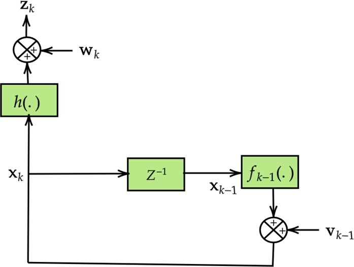
Representation of dynamical system.
Table 3.
Summary of EKF algorithm for nonlinear dynamical system.
| Algorithm 1: Extended Kalman filter. |
|---|
| Initialization: |
| Initialize Pk−1|k−1, , Qk−1 and Rk. |
| Prediction step: |
| Calculate Fk−1 and Lk−1 using (5) and (6) respectively. |
| Calculate predicted mean |
| . |
| Evaluate the predicted covariance Pk|k−1: |
| . |
| Update step: |
| Calculate Hk and Mk using (7) and (8) respectively. |
| Compute the Kalman gain Kk: |
| . |
| Compute estimated mean : |
| . |
| Compute the estimated covariance Pk|k: |
| . |
The EKF algorithm gives the best estimates if following assumptions are fulfilled:
-
•
Matrices and have small norms;
-
•
Initial estimates are equal to actual state of the system;
-
•
Nonlinear functions and are mildly nonlinear functions;
where and denote a prior estimate and post estimate, respectively. I is the identity matrix. The time prediction step consists of computing the state projection and error covariance estimation. Measurement update step (correction step) consists of computing the Kalman gain, state correction, and covariance update. Kalman gain is used to correct the expected state. In this step, observed measurements and expected values are compared for state correction and covariance estimation. The steps involved in the EKF algorithm using flowchart are as shown in Fig. 2 .
Fig. 2.
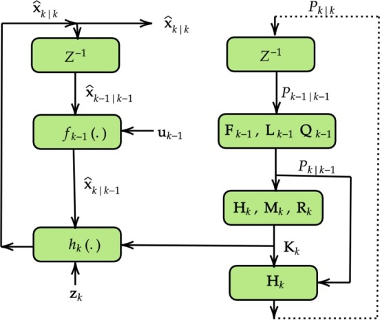
EKF algorithm flowchart.
3. Fractional-order calculus
Fractional order calculus was introduced in 1695 by Leibniz, and it attracted several researchers due to its various advantages. In the literature, mainly, Grünwald-Letnikov, Riemann-Liouville, and Caputo defined fractional-order calculus integral form [33]. Amongst these three, Grünwald-Letnikov definition for fractional-order derivative can be used for state estimation of any nonlinear dynamical system due to its compatibility with various filtering methods [34]. Mathematically, it can be expressed as
| (9) |
where and α denote the integral-differential operator and integral-differential order, respectively. is the memory length. is the Newton Binomial coefficient which is formulated as
| (10) |
where is the Gamma function, mathematically it is expressed as
| (11) |
Continuous time Grünwald-Letnikov fractional-order derivative has the disadvantage that it can not be operated and implemented on computer software as it is infinite dimensional. To get over infinite dimensionality, Grünwald-Letnikov fractional-order derivative is converted to discrete form and reduced to finite dimensional form. Therefore, equation (9) is formulated as
| (12) |
4. State space modeling of BHRP transmission network model
Fig. 3 shows SEIR compartmental model [47], which is based on the clinical progression of the COVID-19. The SEIR model is parameterized in accordance with increase in the number of confirmed cases. The stability of fractional-order SEIR is presented in [48]. Reproduction number denotes the estimated transmission of the disease.
Fig. 3.
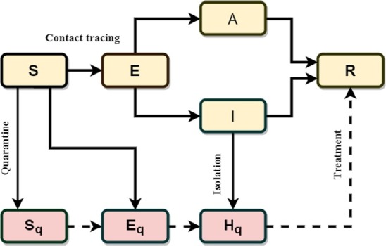
SEIR model.
BHRP model is based on the fact that viruses are transmitted among the bats, and it is transmitted to unknown hosts. These hosts were sent to the seafood market, which was called the reservoir of the COVID-19. Then, it is transmitted to local people, as shown in Fig. 4 . Description of state variables , ... and parameters is as shown in Table 4 and Table 5 respectively. In the proposed generalized SEIR based model, there is the potential presence of unparameterized disease thresholds for both the infected and infectious populations. It should be noted that the total people and infectious people can be directly known by inspecting the day-to-day disease effects by directly taking the required data.
Fig. 4.

BHRP model.
Table 4.
State variable description.
| Source | State variable | Description |
|---|---|---|
| Bat | x1 | Susceptible bats |
| x2 | Exposed bats | |
| x3 | Infected bats | |
| x4 | Removed bats | |
| Hosts | x5 | Susceptible hosts |
| x6 | Exposed hosts | |
| x7 | Infected hosts | |
| x8 | Removed hosts | |
| People | x9 | Susceptible people |
| x10 | Exposed people | |
| x11 | Symptomatic infected people | |
| x12 | Removed people | |
| x13 | Asymptomatic infected people | |
| x14 | SARS-CoV-2 in reservoir | |
Table 5.
Parameter description.
| Source | Parameter | Description |
|---|---|---|
| Bats | nB | Birth rate of bats |
| mB | Death rate of bats | |
| μB | Number of newborn bats | |
| The incubation period of bats | ||
| Infectious period of bats | ||
| Hosts | nH | Birth rate of hosts |
| mH | Death rate of hosts | |
| μH | Number of new hosts | |
| The incubation period of hosts | ||
| Infectious period of hosts | ||
| People | Latent period of people | |
| mP | Death rate of people | |
| The incubation period of people | ||
| Infectious period symptomatic infection of people | ||
| Infectious period asymptomatic infection of people | ||
| Transmission from one source to another source | βB | Transmission rate from infectious bats to susceptible bats |
| βBH | Transmission rate from infectious bats to susceptible hosts | |
| βH | Transmission rate from infectious hosts to susceptible hosts | |
| βP | Transmission rate from infectious people to susceptible people | |
| βW | Transmission rate from infectious people from reservoir to susceptible people | |
| βW | Transmission rate from infectious people from reservoir to susceptible people | |
| Virus lifetime in reservoir | ||
Based on the SEIR model, BHRP model may be obtained. Nonlinear dynamic equations for the SEIR model for bats are
| (13) |
| (14) |
| (15) |
| (16) |
Similarly, dynamic equations for hosts are
| (17) |
| (18) |
| (19) |
| (20) |
Dynamic equations for transmissibility from people are
| (21) |
| (22) |
| (23) |
| (24) |
| (25) |
| (26) |
SIER based model consists of susceptible people (), exposed people (), symptomatic infected people (), asymptomatic infected people (), and removed people () including recovered and death people. The birth rate and death rate of people were defined as and . In this model, we set where denotes the total number of people. The incubation period and latent period of people infection was defined as and .
Total number of infected people due to the COVID-19 are
| (27) |
The above dynamic equations (13) to (27) combined to give BHRP model. Vector form of above BHRP model based fractional-order differential equations are
| (28) |
| (29) |
where ,
where , , , , , , , , , , , , , , .
Consider as reproduction number of infected people of the COVID-19. Using next generation matrix method, we can express for the BHRP model as
| (30) |
Euler-Maruyama method has been used to obtain discrete time state space equation using such that
| (31) |
| (32) |
where is the sampling time [49].
5. Applying EKF to BHRP transmission network model
Discrete time equations of (13)-(26) and (30) in the form of state space model can be formulated as
| (33) |
| (34) |
where
EKF algorithm has been implemented to the discrete equations by adding process noise and measurement noise to (33) and (34) respectively,
| (35) |
| (36) |
6. Kronecker product based fractional-order system representation using WT method
Formalism of the measurement model is
| (37) |
where
denotes the zero mean white Gaussian process. can be expanded using wavelet basis as
| (38) |
where resolution range depends on frequency of operation and the measured time duration and the mother wavelet is given by
| (39) |
Mother wavelet in WT method can be reconstructed from the ‘scaling sequence’ for different type of wavelets (Daubechies wavelet, Haar wavelet, Shannon wavelet etc.) which have specific properties required for specific kinds of applications. Daubechies wavelets are discrete time orthogonal wavelets in which the scaling and the wavelet functions have longer supports, which offers improved capability of these transformations. These transformations offer powerful tool for various signal processing such as compression, noise removal, image enhancement etc. Let mother wavelet range is [a, b], and denote the lowest and the highest frequency of operation. Consider is the measurement time span. Then, for a specified resolution index i, the extent of the transition index k is chosen such that . Therefore, or . Wavelet frequency is mathematically expressed as
| (40) |
where
| (41) |
| (42) |
so the resolution indexes , must be chosen such that
| (43) |
| (44) |
or
| (45) |
| (46) |
Now, resolution index range is selected using this method enables us to reserve lesser data for estimation purpose i.e., estimation is done using compression. The wavelet method is applied either directly to estimate the entire set of the state variables or another way is to formulate a square non-singular matrix. The latter case is formulated as
| (47) |
and so
| (48) |
The signals and are expressed using wavelets as
| (49) |
| (50) |
Substituting (49) and (50) into (48) and neglecting noise terms, we get
| (51) |
where
| (52) |
Now, the inner product is computed with on (51) can be written as
| (53) |
where the input , i.e. . Equation (53) can be formulated as
| (54) |
where , and are formulated in terms of , F, , , . , depend on Θ, so we write
| (55) |
Now, the perturbation method is used to retain terms as
| (56) |
Comparing the coefficients of , , respectively gives
| (57) |
| (58) |
| (59) |
where , and are obtained from WT of , and respectively by equating , and variations expressed in . ⊗ is the Kronecker product of two matrices.
Thus, we can use gradient search algorithm to estimate Θ to minimize
| (60) |
7. Results and discussion
The mathematical model proposed here is a generalized method that can be applied to any population under different scenarios. In this work, we have applied the proposed model to estimate the number of infected and the recovered people due to COVID-19 in India and China. Fig. 5, Fig. 6, Fig. 7, Fig. 8, Fig. 9, Fig. 10, Fig. 11 depict the number of estimated infected people and recovered people using FOC-based EKF method and WT method, and it is compared with the actual number of infected people and recovered people [50]. The values of the parameters used for the estimation are: The incubation period is set to 5.2 days, i.e. 95% confidence interval is 4.1-7.0, , the mean infectious period of the cases as 5.8 days i.e. , . The transmission rate from infectious people to susceptible people () is 0.31. Transmissibility of symptomatic infection is considered to be twice the transmissibility of asymptomatic infection; thus, . . The reproduction number during this period for India and China is found to be 3.85 and 2.74, respectively. Parameters and are controlling the estimation of the infected and the recovered population using EKF and WT method and any change in these parameter values leads to a significant change in the infected and the recovered population. The about fact is as shown in Fig. 5 and Fig. 7, which depict the estimation of infected people and recovered people using EKF and WT method as and change from 0.076 to 0.042 and 0.31 to 0.25, respectively. Change in fractional order parameter value also affecting the estimation as shown in Fig. 6 and Fig. 8.
Fig. 5.

Estimation of infected and recovered people in India using SEIR model based EKF and WT method for γP = 0.076, βP = 0.31. Fractional parameter α = 1. (For interpretation of the colors in the figure(s), the reader is referred to the web version of this article.)
Fig. 6.

Estimation of infected and recovered people in India using SEIR model based EKF and WT method for γP = 0.076, βP = 0.31. Fractional parameter α = 1.82.
Fig. 7.

Estimation of infected and recovered people in India using SEIR model based EKF and WT method for γP = 0.042, βP = 0.25. Fractional parameter α = 1.
Fig. 8.

Estimation of infected and recovered people in India using SEIR model based EKF and WT method for γP = 0.042, βP = 0.25. Fractional parameter α = 1.82.
Fig. 9.

Estimation of infected and recovered people in India using SEIR model based EKF for different value of fractional parameter.
Fig. 10.

Estimation of infected and recovered people in China using SEIR model based EKF and WT method for γP = 0.002, βP = 0.16. Fractional parameter α = 1.82.
Fig. 11.
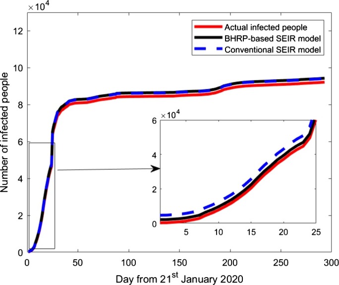
Estimation of infected people using EKF method based on conventional SEIR model and BHRP-based SEIR model.
The comparison of estimation using different values of fractional parameter α is presented in Fig. 9. The fractional-order parameter value gives better estimates as compared to (conventional EKF and WT method). Fig. 10 shows the estimation of infected and recovered people in China using EKF and WT methods for a fixed value of , , and . It is observed that the EKF method gives better estimates than the WT method. A comparison of the proposed BHRP-based SEIR model with the conventional SEIR model for China has been demonstrated in Fig. 11. It is noted that the proposed model outperforms the standard SEIR model for the initial estimation, which further merges with the standard model. This is because, initially, the spreading of coronavirus in China was due to bats, host, and reservoir, so their parameters' effect was more significant. This effect of bats, host, and reservoir parameters got diminished in further spreading of COVID-19 due to the dominance of human transmission. The estimation accuracy of the methods discussed in the preceding sections can be calculated in terms of symmetric mean absolute percentage error (SMAPE) [51] as
| (61) |
where N is the number of samples, and are the cumulative number of cases and estimated number of cases, respectively, for region i at time k. Table 6 and Table 7 show the SMAPE for the estimation of infected and recovered people using EKF and WT methods for India and China for various values of system parameters. It is clear from the results that the FOC-based EKF method gives better performance than the conventional EKF and the WT methods. This is due to the fact that EKF uses the stochastic approach for the estimation; i.e., it considers both the measurement noise and the process noise in which states are Markov process. Moreover, EKF gives the joint evaluation of conditional mean and conditional error covariance; therefore, it gives better estimates.
Table 6.
SMAPE for the estimation of infected people using EKF and WT method.
| Country | Parameter values | EKF method |
WT method |
||||
|---|---|---|---|---|---|---|---|
| India | , | 0.00143 | 0.00138 | 0.00131 | 0.00157 | 0.00154 | 0.00148 |
| India | , | 0.00145 | 0.00140 | 0.00136 | 0.00161 | 0.00162 | 0.00151 |
| India | , | 0.00148 | 0.00145 | 0.00140 | 0.00166 | 0.00164 | 0.00161 |
| China | , | 0.00126 | 0.00118 | 0.00110 | 0.00252 | 0.00248 | 0.00262 |
| China | , | 0.00135 | 0.00120 | 0.00113 | 0.00261 | 0.00257 | 0.00261 |
| China | , | 0.00144 | 0.00131 | 0.00128 | 0.00266 | 0.00264 | 0.00262 |
Table 7.
SMAPE for the estimation of recovered people using EKF and WT method.
| Country | Parameter values | EKF method |
WT method |
||||
|---|---|---|---|---|---|---|---|
| India | , | 0.00150 | 0.00149 | 0.00145 | 0.00170 | 0.00167 | 0.00160 |
| India | , | 0.00153 | 0.00151 | 0.00148 | 0.00173 | 0.00165 | 0.00162 |
| India | , | 0.00160 | 0.00158 | 0.00155 | 0.00175 | 0.00173 | 0.00170 |
| China | , | 0.00137 | 0.00130 | 0.00122 | 0.00264 | 0.00260 | 0.00273 |
| China | , | 0.00145 | 0.00132 | 0.00124 | 0.00269 | 0.00268 | 0.00265 |
| China | , | 0.00156 | 0.00140 | 0.00139 | 0.00276 | 0.00275 | 0.00272 |
General remarks
-
1.When non-Gaussian component is added with the Gaussian distribution of measurement noise, it is called as outlier. EKF can be formulated for this condition also. As EKF is derived from Kushner filter's equation for which the states are Markovian and the measurement noise considered as Gaussian process. When the measurement noise is non-white Gaussian process, nonlinear EKF can be formulated which is based on the Bayesian method for computing the conditional probabilities using non-Gaussian probability density functions. This follows the fact, for non-Gaussian measurement noise, the states are Markovian. First discretize the state model as
(62) (63) (64) (65) (66) (67)
Using these Bayesian arguments, we can develop the nonlinear filter, when states are arbitrary Markovian process and measurement noise is non-Gaussian process. It should be noted that in our notation, is the instantaneous measurement at the time n, while is the aggregate of all measurements taken up to time n.(68) -
2.
Large measurement noise (R) leads to bad estimates in EKF method. However, small value of R leads to large which cause numerical instability. On the other hand, application of gradient search algorithm has computational limitations as matrix is highly nonlinear dependence of parameter Θ.
8. Conclusions
This paper presents the transmissibility and recovery estimation of COVID-19 using the FOC-based EKF and WT methods. The EKF considers measurement and process noise into consideration, which gives better accuracy, while Kronecker product-based WT utilizes the property of scaling/resolution over different-time slots, which results in the compression of data. The importance of proposed models lies in the fact that these models can accommodate conventional EKF and WT methods as their special cases. Further, the estimated number of infected people and recovered people has been compared with the actual number of infected people and recovered people in India and China. Furthermore, the estimation accuracy of the proposed models is obtained in terms of SMAPE forecast errors. It is concluded that the FOC-based EKF method gives better performance than the conventional EKF and WT methods.
CRediT authorship contribution statement
All authors have participated in (a) conception and design, or analysis and interpretation of the data; (b) drafting the article or revising it critically for important intellectual content; and (c) approval of the final version. All the authors have contributed equally to the work reported in the manuscript (e.g., technical help, writing and editing assistance, general support), but who do not meet the criteria for authorship, are named in the Acknowledgements and have given us their written permission to be named. The corresponding author is responsible for ensuring that the descriptions are accurate and agreed by all authors.
Declaration of Competing Interest
The authors declare that they have no known competing financial interests or personal relationships that could have appeared to influence the work reported in this paper.
Biographies

Rahul Bansal received Ph.D. degree from Delhi Technological University (Formerly Delhi College of Engineering), New Delhi, India, in 2020. He was the recipient of Junior Research Fellowship and Senior Research Fellowship from Council for Scientific and Industrial Research (CSIR), India. He received Research Excellence Award from Delhi Technological University, Delhi, India in March 2020. He is a reviewer of several international journals of Springer, IEEE, Elsevier, Taylor & Francis, Emerald. He is currently working as an Assistant Professor with the Department of Electronics and Communication Engineering, Ajay Kumar Garg Engineering College, Ghaziabad, India. His research interests include nonlinear filtering, state and parameter estimation of the systems, nonlinear analysis of systems, stochastic filtering.

Amit Kumar received his Bachelor of Computer Application (BCA) from Dr. Bhimrao Ambedkar University, Agra, India and Master of Computer Application (MCA) from Amity University, Noida, India. Currently, he is working as an Assistant Professor in Dyal Singh College, Delhi University, India. His research interests include parameter estimation of the systems, nonlinear analysis of systems etc.
Amit Kumar Singh received his M.Tech. and Ph.D. degree in Computer Science from Jawaharlal Nehru University, New Delhi, India. He was a postdoc fellow in National Tsing Hua University, Taiwan. He is currently an assistant professor with the department of Computer Science at Ramanujan College, University of Delhi, India. His research interests include performance modeling of wireless networks, information theory, and queueing systems.
Sandeep Kumar received his B. Tech. in electronics and communication from Kurukshetra University, India in 2004 and Master of Engineering in Electronics and Communication from Thapar University, Patiala, India in 2007. He received his Ph.D. from Delhi Technological University, Delhi, India in 2018. He is currently working as Member (Senior Research Staff) at Central Research Laboratory, Bharat Electronics Limited Ghaziabad, India. His research interests include the study of wireless channels, performance modeling of fading channels, cognitive radio networks and parameter estimation of the systems. He is also serving as a reviewer for several international journals of IEEE, Springer, Elsevier etc.
References
- 1.Chen Y., Liu Q., Guo D. Emerging coronaviruses: genome structure, replication, and pathogenesis. J. Med. Virol. 2020;92(4):418–423. doi: 10.1002/jmv.25681. [DOI] [PMC free article] [PubMed] [Google Scholar]
- 2.Carlos W.G., Dela Cruz C.S., Cao B., Pasnick S., Jamil S. Novel Wuhan (2019-nCoV) coronavirus. Am. J. Respir. Crit. Care Med. 2020 doi: 10.1164/rccm.2014P7. [DOI] [PubMed] [Google Scholar]
- 3.Gralinski L.E., Menachery V.D. Return of the coronavirus: 2019-nCoV. Viruses. 2020;12(2) doi: 10.3390/v12020135. [DOI] [PMC free article] [PubMed] [Google Scholar]
- 4.Zhao S., Lin Q., Ran J., et al. Preliminary estimation of the basic reproduction number of novel coronavirus (2019-nCoV) in China, from 2019 to 2020: a data-driven analysis in the early phase of the outbreak. Int. J. Infect. Dis. 2020;92:214–217. doi: 10.1016/j.ijid.2020.01.050. [DOI] [PMC free article] [PubMed] [Google Scholar]
- 5.Li J., Wang Y., Gilmour S., et al. Estimation of the epidemic properties of the 2019, novel coronavirus: a mathematical modeling study. medRxiv. 2020 doi: 10.2139/ssrn.3542150. [DOI] [Google Scholar]
- 6.Lauer S.A., Grantz K.H., Bi Q., et al. The incubation period of coronavirus disease 2019 (COVID-19) from publicly reported confirmed cases: estimation and application. Ann. Intern. Med. 2020;172(9):577–583. doi: 10.7326/M20-0504. [DOI] [PMC free article] [PubMed] [Google Scholar]
- 7.Tang B., Wang X., Li Q., et al. Estimation of the transmission risk of the 2019-nCoV and its implication for public health interventions. J. Clin. Med. 2020;9(2):462. doi: 10.3390/jcm9020462. [DOI] [PMC free article] [PubMed] [Google Scholar]
- 8.Fanelli D., Piazza F. Analysis and forecast of COVID-19 spreading in China, Italy and France. Chaos Solitons Fractals. 2020;134 doi: 10.1016/j.chaos.2020.109761. [DOI] [PMC free article] [PubMed] [Google Scholar]
- 9.Monticelli A. Springer Science & Business Media; 2012. State Estimation in Electric Power Systems: A Generalized Approach. [Google Scholar]
- 10.Zhang Z., Yu Q., Zhang Q., et al. A Kalman filtering based adaptive threshold algorithm for QRS complex detection. Biomed. Signal Process. Control. 2020;58 [Google Scholar]
- 11.Diouf M.L., Iggidr A., Souza M.O. Stability and estimation problems related to a stage-structured epidemic model. Math. Biosci. Eng. 2019;16(5):4415–4432. doi: 10.3934/mbe.2019220. [DOI] [PubMed] [Google Scholar]
- 12.Netto M., Mili L. A robust data-driven Koopman Kalman filter for power systems dynamic state estimation. IEEE Trans. Power Syst. 2018;33(6):7228–7237. [Google Scholar]
- 13.Bansal R., Majumdar S., Parthasarthy H. Stochastic filtering in electromagnetics. IEEE Trans. Antennas Propag. 2020 doi: 10.1109/TAP.2020.3027054. [DOI] [Google Scholar]
- 14.Rigatos G., Wira P., Melkikh A. Nonlinear optimal control for the synchronization of biological neurons under time-delays. Cogn. Neurodyn. 2019;13(1):89–103. doi: 10.1007/s11571-018-9510-4. [DOI] [PMC free article] [PubMed] [Google Scholar]
- 15.Rigatos G., Siano P., Melkikh A. A nonlinear optimal control approach of insulin infusion for blood glucose levels regulation. Intell. Ind. Syst. 2017;3(2):91–102. [Google Scholar]
- 16.Rigatos G. Statistical validation of multi-agent financial models using the H-infinity Kalman filter. Comput. Econ. 2020:1–22. [Google Scholar]
- 17.Hesar H.D., Mohebbi M. Implementation of a square root filtering approach in marginalized particle filters for mixed linear/nonlinear state space models. Int. J. Adapt. Control Signal Process. 2019;33(3):493–511. [Google Scholar]
- 18.Lamien B., Varon L.A., Orlande H.R., et al. State estimation in bioheat transfer: a comparison of particle filter algorithms. Int. J. Numer. Methods Heat Fluid Flow. 2017;27(3):615–638. [Google Scholar]
- 19.Fujita Y., Hiromoto M., Sato T. PARHELIA: particle filter-based heart rate estimation from photoplethysmographic signals during physical exercise. IEEE Trans. Biomed. Eng. 2017;65(1):189–198. doi: 10.1109/TBME.2017.2697911. [DOI] [PubMed] [Google Scholar]
- 20.Feng L., Ding J., Han Y. Improved sliding mode based EKF for the SOC estimation of lithium-ion batteries. Ionics. 2020:1–8. [Google Scholar]
- 21.Bansal R., Majumdar S., Extended Parthasarathy H. Kalman filter based nonlinear system identification described in terms of Kronecker product. AEÜ, Int. J. Electron. Commun. 2019;108:107–117. [Google Scholar]
- 22.Yakoubi M., Hamdi R., Salah M.B. EEG enhancement using extended Kalman filter to train multi-layer perceptron. Biomed. Eng., Appl. Basis Commun. 2019;31(01) [Google Scholar]
- 23.Brovko O., Wiberg D.M., Arena L., et al. The extended Kalman filter as a pulmonary blood flow estimator. Automatica. 1981;17(1):213–220. [Google Scholar]
- 24.Ullah I., Qian S., Deng Z., Lee J.H. Extended Kalman Filter-based localization algorithm by edge computing in Wireless Sensor Networks. Dig. Commun. Netw. 2020 [Google Scholar]
- 25.Ndanguza D., Mbalawata I.S., Haario H., et al. Analysis of bias in an Ebola epidemic model by extended Kalman filter approach. Math. Comput. Simul. 2017;142:113–129. [Google Scholar]
- 26.Gomez-Exposito A., Rosendo-Macias J.A., Gonzalez-Cagigal M.A. 2020 Jan. 1. Monitoring and tracking the evolution of a viral epidemic through nonlinear Kalman filtering: application to the Covid-19 case. medRxiv. [DOI] [PMC free article] [PubMed] [Google Scholar]
- 27.Majumdar S., Parthasarathy H. Wavelet-based transistor parameter estimation. Circuits Syst. Signal Process. 2010;29(5):953–970. [Google Scholar]
- 28.Cartas-Rosado R., Becerra-Luna B., Martinez-Memije R., Infante-Vazquez O., Lerma C., Perez-Grovas H., Rodriguez-Chagolla J.M. Continuous wavelet transform based processing for estimating the power spectrum content of heart rate variability during hemodiafiltration. Biomed. Signal Process. Control. 2020;62 [Google Scholar]
- 29.Tuncer T., Dogan S., Surface Subasi A. EMG signal classification using ternary pattern and discrete wavelet transform based feature extraction for hand movement recognition. Biomed. Signal Process. Control. 2020;58 [Google Scholar]
- 30.Wu C., Magana M.E., Cotilla-Sanchez E. Dynamic frequency and amplitude estimation for three-phase unbalanced power systems using the unscented Kalman filter. IEEE Trans. Instrum. Meas. 2018;68(9):3387–3395. [Google Scholar]
- 31.Metia S., Ha Q.P., Duc H.N., Azzi M. Estimation of power plant emissions with unscented Kalman filter. IEEE J. Sel. Top. Appl. Earth Obs. Remote Sens. 2018;11(8):2763–2772. [Google Scholar]
- 32.Atrsaei A., Salarieh H., Alasty A., Abediny M. Human arm motion tracking by inertial/magnetic sensors using unscented Kalman filter and relative motion constraint. J. Intell. Robot. Syst. 2018;90(1–2):161–170. [Google Scholar]
- 33.Baleanu D., Diethelm K., Scalas E., Trujillo J.J. World Scientific; Singapore: 2010. Fractional Calculus: Models and Numerical Methods. [Google Scholar]
- 34.Hu X., Yuan H., Zou C., Li Z., Zhang L. Co-estimation of state of charge and state of health for lithium-ion batteries based on fractional-order calculus. IEEE Trans. Veh. Technol. 2018;67(11):10319–10329. [Google Scholar]
- 35.Miljkovic N., Popovic N., Djordjevic O., Konstantinovic L., Sekara T.B. ECG artifact cancellation in surface EMG signals by fractional order calculus application. Comput. Methods Programs Biomed. 2017;140:259–264. doi: 10.1016/j.cmpb.2016.12.017. [DOI] [PubMed] [Google Scholar]
- 36.Popovic N.B., Miljkovic N., Sekara T.B. Electrogastrogram and electrocardiogram interference: Application of fractional order calculus and Savitzky-Golay filter for biosignals segregation. 2020 19th International Symposium INFOTEH-JAHORINA; INFOTEH; IEEE; 2020. pp. 1–5. Mar 18. [Google Scholar]
- 37.Rihan F.A., Al-Mdallal Q.M., AlSakaji H.J., Hashish A. A fractional-order epidemic model with time-delay and nonlinear incidence rate. Chaos Solitons Fractals. 2019;126:97–105. [Google Scholar]
- 38.Rihan F.A., Baleanu D., Lakshmanan S., Rakkiyappan R. On fractional SIRC model with salmonella bacterial infection. Abstract and Applied Analysis; Hindawi; 2014 Apr 1. (Vol. 2014) [Google Scholar]
- 39.Latha V.P., Rihan F.A., Rakkiyappan R., Velmurugan G. A fractional-order model for Ebola virus infection with delayed immune response on heterogeneous complex networks. Am. J. Comput. Appl. Math. 2018;339:134–146. [Google Scholar]
- 40.Mawonou K.S., Eddahech A., Dumur D., Beauvois D., Godoy E. Improved state of charge estimation for Li-ion batteries using fractional order extended Kalman filter. J. Power Sources. 2019;435 [Google Scholar]
- 41.Hidalgo-Reyes J.I., Gomez-Aguilar J.F., Alvarado-Martinez V.M., Lopez-Lopez M.G., Escobar-Jimenez R.F. Battery state-of-charge estimation using fractional extended Kalman filter with Mittag-Leffler memory. Alex. Eng. J. 2019 [Google Scholar]
- 42.Wang Y., Gao G., Li X., Chen Z. A fractional-order model-based state estimation approach for lithium-ion battery and ultra-capacitor hybrid power source system considering load trajectory. J. Power Sources. 2020;449 [Google Scholar]
- 43.Huang X., Gao Z., Yang C., Liu F. State estimation of continuous-time linear fractional-order systems disturbed by correlated colored noises via Tustin generating function. IEEE Access. 2020;8:18362–18373. [Google Scholar]
- 44.Brewer J. Kronecker products and matrix calculus in system theory. IEEE Trans. Circuits Syst. 1978;25(9):772–781. [Google Scholar]
- 45.Greub W.H. Springer; Berlin, Heidelberg: 1967. Multilinear Algebra. [Google Scholar]
- 46.Chen T., Rui J., Wang Q., Zhao Z., Cui J-A., Yin L. 2020. A mathematical model for simulating the transmission of Wuhan novel Coronavirus.2020.2001.2019.911669 bioRxiv. [DOI] [PMC free article] [PubMed] [Google Scholar]
- 47.Zha W.T., Pang F.R., Zhou N., Wu B., Liu Y., Du Y.B., Hong X.Q., Lv Y. Research about the optimal strategies for prevention and control of varicella outbreak in a school in a central city of China: based on an SEIR dynamic model. Epidemiol. Infect. 2020:148. doi: 10.1017/S0950268819002188. [DOI] [PMC free article] [PubMed] [Google Scholar]
- 48.Yang Y., Xu L. Stability of a fractional order SEIR model with general incidence. Appl. Math. Lett. 2020;24 [Google Scholar]
- 49.Xiong B., Zhao J., Wei Z., et al. Extended Kalman filter method for state of charge estimation of vanadium redox flow battery using thermal-dependent electrical model. J. Power Sources. 2014;262:50–61. [Google Scholar]
- 50.World Health Organization . World Health Organization; 2020. Novel Coronavirus.https://www.who.int/ Available at. [Google Scholar]
- 51.Hyndman R.J., Koehler A.B. Another look at measures of forecast accuracy. Int. J. Forecast. 2006;22(4):679–688. [Google Scholar]