DE69727505T2 - GENERATION OF PROTOTYPE SIGNALS FOR MULTI-CARRIER TRANSMISSION - Google Patents
GENERATION OF PROTOTYPE SIGNALS FOR MULTI-CARRIER TRANSMISSION Download PDFInfo
- Publication number
- DE69727505T2 DE69727505T2 DE69727505T DE69727505T DE69727505T2 DE 69727505 T2 DE69727505 T2 DE 69727505T2 DE 69727505 T DE69727505 T DE 69727505T DE 69727505 T DE69727505 T DE 69727505T DE 69727505 T2 DE69727505 T2 DE 69727505T2
- Authority
- DE
- Germany
- Prior art keywords
- function
- frequency
- signal
- time
- ofdm
- Prior art date
- Legal status (The legal status is an assumption and is not a legal conclusion. Google has not performed a legal analysis and makes no representation as to the accuracy of the status listed.)
- Expired - Lifetime
Links
- 230000005540 biological transmission Effects 0.000 title claims abstract description 28
- 230000006870 function Effects 0.000 claims description 298
- 238000000034 method Methods 0.000 claims description 36
- 230000004044 response Effects 0.000 claims description 23
- 238000010276 construction Methods 0.000 claims description 19
- 238000012937 correction Methods 0.000 claims description 9
- 238000001914 filtration Methods 0.000 claims description 9
- 238000001228 spectrum Methods 0.000 claims description 7
- 239000000969 carrier Substances 0.000 abstract description 3
- 239000013598 vector Substances 0.000 description 20
- 238000004422 calculation algorithm Methods 0.000 description 18
- 239000011159 matrix material Substances 0.000 description 16
- 230000007423 decrease Effects 0.000 description 15
- 238000012545 processing Methods 0.000 description 14
- 238000012546 transfer Methods 0.000 description 12
- 230000002123 temporal effect Effects 0.000 description 10
- 238000013459 approach Methods 0.000 description 8
- 230000008859 change Effects 0.000 description 8
- 238000005516 engineering process Methods 0.000 description 8
- 230000009466 transformation Effects 0.000 description 8
- 238000009826 distribution Methods 0.000 description 7
- 230000003595 spectral effect Effects 0.000 description 7
- 230000035945 sensitivity Effects 0.000 description 6
- 230000008901 benefit Effects 0.000 description 5
- 238000005562 fading Methods 0.000 description 5
- 230000010363 phase shift Effects 0.000 description 5
- 230000006399 behavior Effects 0.000 description 4
- 238000004364 calculation method Methods 0.000 description 4
- 238000000354 decomposition reaction Methods 0.000 description 4
- 238000013461 design Methods 0.000 description 4
- 230000009977 dual effect Effects 0.000 description 4
- 238000007429 general method Methods 0.000 description 4
- 230000004807 localization Effects 0.000 description 4
- 230000000737 periodic effect Effects 0.000 description 4
- 230000009471 action Effects 0.000 description 3
- 238000011161 development Methods 0.000 description 3
- 230000000694 effects Effects 0.000 description 3
- 238000013507 mapping Methods 0.000 description 3
- 230000036961 partial effect Effects 0.000 description 3
- 238000005070 sampling Methods 0.000 description 3
- 230000003068 static effect Effects 0.000 description 3
- 230000001360 synchronised effect Effects 0.000 description 3
- 238000006243 chemical reaction Methods 0.000 description 2
- 238000004891 communication Methods 0.000 description 2
- ZINJLDJMHCUBIP-UHFFFAOYSA-N ethametsulfuron-methyl Chemical compound CCOC1=NC(NC)=NC(NC(=O)NS(=O)(=O)C=2C(=CC=CC=2)C(=O)OC)=N1 ZINJLDJMHCUBIP-UHFFFAOYSA-N 0.000 description 2
- 238000004321 preservation Methods 0.000 description 2
- 230000008569 process Effects 0.000 description 2
- 230000002829 reductive effect Effects 0.000 description 2
- 241000195493 Cryptophyta Species 0.000 description 1
- 241000196324 Embryophyta Species 0.000 description 1
- 240000007594 Oryza sativa Species 0.000 description 1
- 235000007164 Oryza sativa Nutrition 0.000 description 1
- 239000000654 additive Substances 0.000 description 1
- 230000000996 additive effect Effects 0.000 description 1
- 238000004458 analytical method Methods 0.000 description 1
- 238000009411 base construction Methods 0.000 description 1
- 230000015556 catabolic process Effects 0.000 description 1
- 238000010835 comparative analysis Methods 0.000 description 1
- 230000001419 dependent effect Effects 0.000 description 1
- 238000006073 displacement reaction Methods 0.000 description 1
- HVCNNTAUBZIYCG-UHFFFAOYSA-N ethyl 2-[4-[(6-chloro-1,3-benzothiazol-2-yl)oxy]phenoxy]propanoate Chemical compound C1=CC(OC(C)C(=O)OCC)=CC=C1OC1=NC2=CC=C(Cl)C=C2S1 HVCNNTAUBZIYCG-UHFFFAOYSA-N 0.000 description 1
- 238000011156 evaluation Methods 0.000 description 1
- 230000010354 integration Effects 0.000 description 1
- 230000000670 limiting effect Effects 0.000 description 1
- 230000005923 long-lasting effect Effects 0.000 description 1
- 230000015654 memory Effects 0.000 description 1
- 238000010606 normalization Methods 0.000 description 1
- 230000001681 protective effect Effects 0.000 description 1
- 235000009566 rice Nutrition 0.000 description 1
- 238000007493 shaping process Methods 0.000 description 1
- 241000894007 species Species 0.000 description 1
- 230000007480 spreading Effects 0.000 description 1
- 238000001356 surgical procedure Methods 0.000 description 1
- 230000029305 taxis Effects 0.000 description 1
- 238000000844 transformation Methods 0.000 description 1
- 230000007704 transition Effects 0.000 description 1
- XLYOFNOQVPJJNP-UHFFFAOYSA-N water Substances O XLYOFNOQVPJJNP-UHFFFAOYSA-N 0.000 description 1
Classifications
-
- H—ELECTRICITY
- H04—ELECTRIC COMMUNICATION TECHNIQUE
- H04L—TRANSMISSION OF DIGITAL INFORMATION, e.g. TELEGRAPHIC COMMUNICATION
- H04L27/00—Modulated-carrier systems
- H04L27/26—Systems using multi-frequency codes
- H04L27/2601—Multicarrier modulation systems
- H04L27/2602—Signal structure
-
- H—ELECTRICITY
- H04—ELECTRIC COMMUNICATION TECHNIQUE
- H04L—TRANSMISSION OF DIGITAL INFORMATION, e.g. TELEGRAPHIC COMMUNICATION
- H04L27/00—Modulated-carrier systems
- H04L27/26—Systems using multi-frequency codes
- H04L27/2601—Multicarrier modulation systems
- H04L27/2626—Arrangements specific to the transmitter only
- H04L27/2627—Modulators
- H04L27/264—Pulse-shaped multi-carrier, i.e. not using rectangular window
- H04L27/26416—Filtering per subcarrier, e.g. filterbank multicarrier [FBMC]
-
- H—ELECTRICITY
- H04—ELECTRIC COMMUNICATION TECHNIQUE
- H04L—TRANSMISSION OF DIGITAL INFORMATION, e.g. TELEGRAPHIC COMMUNICATION
- H04L27/00—Modulated-carrier systems
- H04L27/26—Systems using multi-frequency codes
- H04L27/2601—Multicarrier modulation systems
- H04L27/2697—Multicarrier modulation systems in combination with other modulation techniques
- H04L27/2698—Multicarrier modulation systems in combination with other modulation techniques double density OFDM/OQAM system, e.g. OFDM/OQAM-IOTA system
-
- H—ELECTRICITY
- H04—ELECTRIC COMMUNICATION TECHNIQUE
- H04L—TRANSMISSION OF DIGITAL INFORMATION, e.g. TELEGRAPHIC COMMUNICATION
- H04L27/00—Modulated-carrier systems
- H04L27/26—Systems using multi-frequency codes
- H04L27/2601—Multicarrier modulation systems
- H04L27/2647—Arrangements specific to the receiver only
- H04L27/2649—Demodulators
- H04L27/26534—Pulse-shaped multi-carrier, i.e. not using rectangular window
- H04L27/2654—Filtering per subcarrier, e.g. filterbank multicarrier [FBMC]
Landscapes
- Engineering & Computer Science (AREA)
- Computer Networks & Wireless Communication (AREA)
- Signal Processing (AREA)
- Digital Transmission Methods That Use Modulated Carrier Waves (AREA)
- Reduction Or Emphasis Of Bandwidth Of Signals (AREA)
- Mobile Radio Communication Systems (AREA)
Abstract
Description
1. Erfindungsbereich1. Area of invention
1.1 Allgemeiner Bereich1.1 General area
Der Erfindungsbereich ist der des Sendens oder der Übertragung von digitalen Daten oder analoger und abgetasteter Daten, die insbesondere durch mobile Stationen empfangen werden sollen. Genauer gesagt betrifft die Erfindung Signale, die mit Hilfe neuer Modulationen sowie mit den entsprechenden Modulations- und Demodulationstechniken erzeugt werden.The The scope of the invention is that of transmitting or transmitting digital data or analog and sampled data, in particular through mobile Stations are to be received. More specifically, the invention relates to Signals with the help of new modulations as well as with the corresponding ones Modulation and demodulation techniques are generated.
Seit vielen Jahren versucht man, Modulationen zu konstruieren, die stark unstationären Kanälen angepasst sind, beispielsweise Sendekanäle zu mobilen Stationen. In solchen Kanälen ist das gesendete Signal von Fading und Mehrwegeausbreitungen betroffen. Die von der CCETT im Rahmen des europäischen Projektes EUREKA 147 durchgeführten Arbeiten (DAB: Digital Audio Broadcasting oder Audiodigitales Senden) haben gezeigt, dass für diese Art von Kanälen, Mehrträger-Modulationen von Interesse sind und insbesondere das OFDM (Orthogonal Frequency Division Multiplexing, Orthogonales Frequenz-Multiplex).since For many years one tries to construct modulations that are strong unstationären channels are adapted, for example transmission channels to mobile stations. In such channels the transmitted signal is affected by fading and multipath propagation. The CCETT as part of the European project EUREKA 147 conducted Working (DAB: digital audio broadcasting or audio digital broadcasting) have shown that for these types of channels Multi-carrier modulations are of interest and especially the OFDM (Orthogonal Frequency Multiplexing division, orthogonal frequency division multiplex).
Das OFDM wurde im Rahmen dieses europäischen Projektes als Basis der DAB-Norm gewählt. Diese Technik wurde ebenfalls als Modulation für das Senden von Fernsehprogrammen (DVB) gewählt. Man stellt jedoch fest, dass es eine Reihe von Beschränkungen gibt (die weiter vorne genauer erläutert werden), wenn man das Problem von mit hoher spektralen Leistungsfähigkeit kodierten Modulationen angeht, wie beispielsweise von digitalen Fernsehanwendungen verlangt.The OFDM was used as the basis for this European project of the DAB standard. This technique was also used as a modulation for broadcasting TV programs (DVB) selected. However, it is found that there are a number of restrictions there (which are explained in more detail above) if you do that Problem of modulations coded with high spectral performance as required by digital television applications.
1.2 Mögliche Anwendungen1.2 Possible applications
Die Erfindung findet Anwendungen in sehr verschiedenen Bereichen, insbesondere dann, wenn eine hohe spektrale Leistungsfähigkeit gewünscht wird und der Kanal stark unstationär ist.The Invention finds applications in very different fields, in particular when high spectral performance is desired and the channel is strong unstationär is.
Eine erste Kategorie von Anwendungen betrifft terrestrische digitale Funkverbindungen, sowohl für Bilder als auch für Ton und/oder Daten. Insbesondere kann die Erfindung das synchrone Senden betreffen, das in inhärenter Weise lang andauernde Mehrwegeausbreitungen erzeugt. Sie betrifft ebenfalls vorteilhafterweise das Senden zu mobilen Stationen.A first category of applications concerns terrestrial digital Radio connections, both for Pictures as well for Sound and / or data. In particular, the invention can synchronous Sending concern that is inherent Generated long-lasting multipath propagation. It affects also advantageously sending to mobile stations.
Eine andere Kategorie von Anwendungen betrifft digitale Funkkommunikationen. Die Erfindung kann insbesondere in digitalen Kommunikationssystemen zu mobilen Stationen mit hohem Durchsatz, beispielsweise im Rahmen von UMTS, zur Anwendung kommen. Sie kann ebenfalls für lokale Funknetze mit hohem Durchsatz (vom Typ HIPERLAN) ins Auge gefasst werden.A another category of applications relates to digital radio communications. The invention can be used in particular in digital communication systems to mobile stations with high throughput, for example in the frame from UMTS. It can also be used for local High throughput radio networks (of the HIPERLAN type) envisaged become.
Eine dritte Kategorie von Anwendungen sind Unterwasserverbindungen. Bei der Unterwasserakustik ist der Sendekanal stark gestört, aufgrund der geringen Fortpflanzungsgeschwindigkeit der Schallwellen im Wasser. Dies bewirkt eine starke Ausbreitung der Mehrwegeausbreitungen und des Doppler-Spektrums. Mehrfachträger-Modulationstechniken sind demnach diesem Bereich gut angepasst und insbesondere die Techniken, die Gegenstand dieser Erfindung sind.A third category of applications are underwater connections. at Due to the underwater acoustics, the transmission channel is severely disturbed the low propagation speed of sound waves in water. This causes the multipath and spread to spread of the Doppler spectrum. Multi-carrier modulation techniques are accordingly well adapted to this area and in particular the techniques which are the subject of this invention.
2. Stand der Technik2. State of the technology
2.1 Theoretische Bemerkungen zur Darstellung von Signalen2.1 Theoretical comments for displaying signals
Bevor man die Signale nach der Erfindung vorstellt, werden nachfolgend die bekannten Signale beschrieben. Diese Beschreibung beruht auf einem allgemeinen Ansatz bezüglich der von den Erfindern definierten Mehrfachträgersignalen, der an sich neu ist. Diese Verallgemeinerung hat nämlich kein Gegenstück im Stand der Technik und ist für den Fachmann keineswegs selbstverständlich. Sie muss demnach als Teil der Erfindung betrachtet werden und nicht als Teil des Standes der Technik.Before the signals according to the invention are presented below the known signals described. This description is based on a general approach to the multi-carrier signals defined by the inventors, which is new per se is. This generalization has no counterpart in the state of technology and is for by no means a matter of course for the specialist. Accordingly, it must be as Be considered part of the invention and not part of the prior art of the technique.
Man
interessiert sich für
reelle Signale (beispielsweise eine elektrische Größe), mit
endlicher Energie, die Funktion der Zeit sind. Die Signale lassen
sich demnach durch reelle Funktionen von L2(R)
darstellen. Ferner weisen diese Signale ein begrenztes Band auf
und ihr Spektrum ist in![]()
![]()
![]()
![]()
Das Signal s(t) gehört einem vektoriellen Teilraum an (charakterisiert durch die Bandbeschränkung auf ±w/2) des Raumes der komplexen Funktionen einer reellen Variable mit summierbarem Quadrat L2(R). Dieser vektorielle Raum kann in zwei verschiedenen Weisen definiert werden, je nachdem ob man auf dem Körper der komplexen oder der reellen Zahlen aufbaut. Jedem Raum kann man ein Skalarprodukt mit einem Wert in C oder R zuordnen und einen Hilbert-Raum konstruieren. Man nennt H den auf dem Körper der komplexen Zahlen aufgebauten Hilbert-Raum und HR den auf dem Körper der komplexen Zahlen aufgebauten Hilbert-Raum.The signal s (t) belongs to a vectorial subspace (characterized by the band restriction to ± w / 2) of the space of the complex functions of a real variable with a summable square L 2 (R). This vectorial space can be defined in two different ways, depending on whether you are building on the body of complex or real numbers. A scalar product with a value in C or R can be assigned to each space and a Hilbert space can be constructed. H is called the Hilbert space built on the body of the complex numbers and H R the Hilbert space built on the body of the complex numbers.
Die entsprechenden Skalarprodukte schreibt man:The corresponding scalar products are written:

Die damit zusammenhängenden Normen sind offensichtlich in beiden Fällen identisch:The related Standards are obviously identical in both cases:
![]()
![]()
2.2 Allgemeine Prinzipien des OFDM2.2 General principles of the OFDM
Die allgemeinen Prinzipien des OFDM werden beispielsweise in dem am 2. Juli 1986 eingereichten französischen Patent FR-86 09622 vorgestellt. Die Grundidee dieser Technik besteht darin, kodierte Symbole als Formkoeffizienten elementarer Wellen zu senden, die so weit wie möglich im Zeit-Frequenz-Raum eingeschränkt sind und für welche der Sendekanal als örtlich stationär angesehen werden kann. Der Kanal erscheint dann als einfacher multiplikativer Kanal, gekennzeichnet durch die Verteilung des Koeffizientenmoduls, der einem Rice- bzw. ein Rayleigh-Gesetz folgt.The General principles of OFDM are described, for example, in the am French filed July 2, 1986 Patent FR-86 09622 presented. The basic idea of this technique is therein, encoded symbols as shape coefficients of elementary waves send that as much as possible restricted in time-frequency space are and for which the broadcast channel as local stationary can be viewed. The channel then appears as a simple multiplicative Channel, characterized by the distribution of the coefficient module, which follows a Rice or Rayleigh law.
Der Schutz gegen Fading wird dann mit Hilfe eines Codes sichergestellt, der unter gewichteter Entscheidung einsetzbar ist, durch Assoziierung mit einer Zeit- und Frequenzverschachtelung, die garantiert, dass die im Minimalgitter des Codes intervenierenden Symbole so weit wie möglich von unabhängigen Fadingvorgängen betroffen sind.The Protection against fading is then ensured with the help of a code, which can be used under weighted decision, through association with a time and Frequency interleaving that guarantees that in the minimum grating symbols intervening in the code as far as possible affected by independent fading are.
Diese Technik mit Verschachtelung im Zeit-Frequenz-Raum ist unter dem Namen COFDM bekannt. Sie ist beispielsweise im Dokument [22] beschrieben (s. Anhang 1 (um das Lesen zu erleichtern sind die meisten Referenzen zum Stand der Technik in diesem Anhang 1 aufgelistet. Dieser Anhang sowie die Anhänge 2 und 3 müssen selbstverständlich als vollwertige Teile dieser Beschreibung angesehen werden)).This Technique with nesting in the time-frequency space is below that Name known as COFDM. It is described, for example, in document [22] (see Appendix 1 (most references are to make reading easier state of the art in this Appendix 1 listed. This appendix as well as the attachments 2 and 3 must Of course are regarded as full parts of this description)).
Es gibt im wesentlichen zwei Arten bekannter OFDM-Modulationen. Da die in der Literatur verwendeten Bezeichnungen des öfteren nicht eindeutig sind, führen wir hier neue und genauere Bezeichnungen ein, wobei wir auf die Zusammenhänge mit der vorhandenen Literatur hinweisen. Die Grundbezeichnung OFDM benutzen wir gefolgt von einem Suffix, der die Art der Modulation innerhalb dieser Familie präzisiert.It are essentially two types of known OFDM modulations. There the designations used in the literature are often not are clear, lead we’re going to add new and more accurate names, relationships with the available literature. Use the basic designation OFDM we followed by a suffix indicating the type of modulation within this family specified.
2.3 OFDM/QAM2.3 OFDM / QAM
2.3.1 Theoretische Prinzipien2.3.1 Theoretical principles
Eine erste Kategorie von Modulationen besteht aus einem Multiplex von QAM-Trägerwellen (Quadrature Amplitude Modulation) bzw. eventuell von Modulationen nach QPSK (Quadrature Phase Shift Keying) für den besonderen Fall von binären Daten. Im Nachfolgenden werden wir dieses System unter dem Namen OFDM/QAM bezeichnen. Die Trägerwellen sind alle synchronisiert und die Entfernungen zwischen Trägerfrequenzen betragen den Umkehrwert der Symbolzeit. Obwohl sich die Spektren dieser Trägerwellen überlappen, erlaubt es die Systemsynchronisierung, die Orthogonalität zwischen den von den verschiedenen Trägerwellen gesendeten Symbolen zu gewährleisten.A first category of modulations consists of a multiplex of QAM carrier waves (Quadrature Amplitude Modulation) or possibly of modulations according to QPSK (Quadrature Phase Shift Keying) for the special case of binary data. In the following we will refer to this system as OFDM / QAM describe. The carrier waves are all synchronized and the distances between carrier frequencies are the inverse of the symbol time. Although the spectra of these carrier waves overlap, allowed it the system synchronization, the orthogonality between those of the different ones Carrier waves sent Ensure symbols.
Die Referenzen [1] bis [7] geben eine gute Übersicht der diesbezüglich verfügbaren Literatur.The References [1] to [7] provide a good overview of the literature available in this regard.
Für mehr Einfachheit beim Schreiben und dem neuen Ansatz der Erfindung entsprechend werden die Signale in ihrer oben beschriebenen analytischen Form dargestellt. Unter diesen Bedingungen wird die allgemeine Gleichung eines OFDM/QAM Signals wie folgt geschrieben:For more simplicity in writing and in accordance with the new approach of the invention the signals are presented in the analytical form described above. Under these conditions, the general equation of an OFDM / QAM Signals written as follows:
![]()
![]()
Die
Koeffizienten am,n nehmen komplexe Werte
an, welche die gesendeten Daten beschreiben. Die Funktionen xm,n(t) sind im Zeit-Frequenz-Raum verschobene
Werte einer selben Prototypfunktion x(t): 
Unter
diesen Bedingungen stellt man folgendes fest:
Die Baryzentren der Grundfunktionen bilden somit ein Gitter der Zeit-Frequenz-Ebene, das von den Vektoren (τ0, 0) und (0, ν0) erzeugt wird. Dieses Gitter weist Einheitsdichte auf, d. h., ν0τ0 = 1. Eine mehr ins Detail gehende Diskussion dieses Themas ist im Artikel [9] zu finden.The barycenters of the basic functions thus form a grid of the time-frequency level, which is generated by the vectors (τ 0 , 0) and (0, ν 0 ). This grid has unit density, ie, ν 0 τ 0 = 1. A more detailed discussion of this topic can be found in Article [9].
Die Prototypfunktion x(t) hat die Besonderheit, dass die Funktionen {xm,n} untereinander orthogonal sind. Genauer bilden sie eine Hilbert'sche Basis von L2(R), oder:The prototype function x (t) has the special feature that the functions {x m, n } are mutually orthogonal. More precisely, they form a Hilbert base of L 2 (R), or:

Das Projizieren eines Signals unter dieser Basis entspricht einfach dem Zerlegen des Signals in Folgen der Dauer τ0 und im Darstellen aller dieser Folgen durch die entsprechende Entwicklung nach einer Fourier-Reihe. Diese Art der Zerlegung bildet einen ersten Schritt in Richtung auf eine gleichzeitige Lokalisierung nach Zeit und Frequenz, im Gegensatz zur klassischen Fourier- Analyse, die eine perfekte Frequenz-Lokalisierung gewährleistet, bei vollkommenem Verlust der Zeitinformation.The projection of a signal under this basis corresponds simply to the decomposition of the signal into sequences of the duration τ 0 and the representation of all of these sequences by the corresponding development after a Fou rier series. This type of decomposition forms a first step towards simultaneous localization according to time and frequency, in contrast to the classic Fourier analysis, which ensures perfect frequency localization with complete loss of time information.
Ist die zeitliche Lokalisierung perfekt, so ist leider die Frequenz-Lokalisierung viel schlechter, aufgrund der langsamen Abnahme von X(f). Der Satz von Balian-Low-Coifman-Semmes (s. [9], S. 976) zeigt außerdem, dass wenn man X als die Fouriertransformierte von x bezeichnet, so können tx(t) und fX(f) nicht gleichzeitig quadratisch summierbar sein.is the temporal localization is perfect, so is the frequency localization much worse, due to the slow decrease in X (f). The sentence from Balian-Low-Coifman-Semmes (see [9], p. 976) also shows that if one denotes X as the Fourier transform of x, then tx (t) and fX (f) cannot be summed quadratic at the same time.
2.3.2 Das OFDM/QAM mit Schutzintervall2.3.2 The OFDM / QAM with guard interval
Allgemein
kann man die Toleranz einer OFDM-Modulation gegenüber Mehrwegeausbreitung
und Doppler-Ausweitung durch einen Parameter charakterisieren, der
in globaler Weise die Variation des Interferenzniveaus zwischen
Symbolen (IES) als Funktion einer Zeit- oder Frequenzverschiebung
misst. Die Begründung
dieses Konzeptes findet man im Anhang 2. Dieser Toleranzparameter
wird ξ genannt
und wird durch die folgende Beziehung definiert:
Aufgrund der Heisenberg'schen Unschärferelation, kann ξ nicht größer als die Einheit sein.by virtue of Heisenberg's Uncertainty principle, can't ξ larger than be the unit.
Aufgrund des oben erwähnten Satzes von Balian-Low-Coifman-Semmes, nimmt der Parameter ξ den Wert 0 für das OFDM/QAM an. Das ist ein schwerwiegender Fehler der OFDM/QAM-Modulation in der oben beschriebenen Form. Dies macht sich in der Praxis durch eine starke Empfindlichkeit gegenüber Zeitfehlern und somit den Mehrwegeausbreitungen bemerkbar.by virtue of of the above Balian-Low-Coifman-Semmes theorem, the parameter ξ takes the value 0 for that OFDM / QAM. This is a serious error in OFDM / QAM modulation in the form described above. This is going through in practice a strong sensitivity to time errors and thus the Multipath propagation noticeable.
Dieser Fehler lässt sich durch Anwendung eines beispielsweise in [5] beschriebenen Schutzintervalls umgehen. Es handelt sich dabei um einen Kunstgriff, bei dem das rechteckige Fenster der Prototypfunktion verlängert wird. Die Dichte des Basissymbolgitters ist dann streng kleiner als die Einheit.This Leaves mistakes circumvent themselves by using a protection interval described, for example, in [5]. It is an artifice in which the rectangular Prototype window is extended. The density of the The base symbol grid is then strictly smaller than the unit.
Diese Technik ist möglich, weil man im Inneren eines durch ein Schutzintervall verlängerten Symbols eine unendliche Zahl von verschobenen Versionen des Ausgangssymbols findet. Dies funktioniert selbstverständlich nur deshalb, weil die Prototypfunktion ein rechteckiges Fenster ist. In diesem Sinne bildet das OFDM/QAM mit Schutzintervall einen einzigen Sonderpunkt.This Technology is possible because one inside is extended by a guard interval Symbol an infinite number of shifted versions of the source symbol place. Of course, this only works because the Prototype function is a rectangular window. With this in mind the OFDM / QAM with protection interval a single special point.
Die OFDM/QAM-Modulation mit Schutzintervall bildet die Basis des DAB-Systems. Dieses Schutzintervall ermöglicht es, die Interferenz zwischen Symbolen um den Preis eines Leistungsverlustes zu begrenzen, da ein Teil der gesendeten Information nicht wirklich vom Empfänger genutzt wird, sondern nur zum Aufnehmen der Mehrwegeausbreitungen dient.The OFDM / QAM modulation with protection interval forms the basis of the DAB system. This guard interval allows it, the interference between symbols at the cost of a loss of performance limit since part of the information sent is not really from the recipient is used, but only to record the multipath propagation serves.
So beträgt im Falle des DAB-Systems, bei dem das Schutzintervall 25% des nützlichen Symbols beträgt, der Verlust 1 dB. Es gibt darüber hinaus einen zusätzlichen Verlust aufgrund der Tatsache, dass, um einen gegebenen gesamten spektralen Wirkungsgrad zu erzielen, der vom Schutzintervall verursachte Verlust durch einen besseren Wirkungsgrad des verwendeten Codes ausgeglichen werden muss.So is in the case of the DAB system, where the guard interval is 25% of the useful Symbol, the loss 1 dB. There's about it an additional one Loss due to the fact that to a given total to achieve spectral efficiency caused by the guard interval Loss due to better efficiency of the code used must be balanced.
Dieser Verlust ist im Falle des DAB-Systems nebensächlich, aufgrund des schwachen spektralen Wirkungsgrades. Peilt man dagegen einen gesamten spektralen Wirkungsgrad von 4 Bits/Hz an, so muss man einen Code mit 5 Bits/Hz verwenden, was nach dem Satz von Shannon, einen Verlust in der Größenordnung von 3 dB bedeutet. Der Gesamtverlust liegt in diesem Falle in etwa bei 4 dB.This Loss is secondary in the case of the DAB system due to the weak one spectral efficiency. On the other hand, if you take an entire spectral range Efficiency of 4 bits / Hz, you have to enter a code with 5 bits / Hz use what, according to Shannon's theorem, is a loss on the order of 3 dB means. The total loss in this case is approximately 4 dB.
2.3.3 Andere OFDM/QAM-Systeme2.3.3 Other OFDM / QAM systems
Es sind andere Systeme vom Typ OFDM/QAM denkbar. Leider erfüllt keine gefilterte QAM-Modulation (d. h., eine Modulation, die eine konventionelle Formgebung des Typs Halb-Nyquist (oder genauer gesagt, „Quadratwurzel von Nyquist") verwendet) die erforderlichen Orthogonalitäts-Zwänge. Die bekannten Prototypfunktionen, welche die erforderlichen Orthogonalitätskriterien erfüllen, sind:
- – das rechteckige Fenster;
- – der Cardinalsinus.
- - the rectangular window;
- - the cardinal sine.
Diese zwei Beispiele sind trivial und erscheinen gegenseitig dual durch Fouriertransformierte. Der Fall des rechteckigen Fensters entspricht dem OFDM/QAM ohne Schutzintervall. Der Fall des Cardinalsinus entspricht einem klassischen Frequenzmultiplex (d. h., bei dem die Trägerfrequenzen voneinander getrennte Spektren aufweisen), mit einem Roll-off von 0%, was einen in der Praxis schwer zu verwirklichenden asymptotischen Fall darstellt.This two examples are trivial and appear dual to each other Fourier transform. The case of the rectangular window corresponds the OFDM / QAM without protection interval. The case of the cardinal sinus corresponds a classic frequency division multiplex (i.e. where the carrier frequencies have separate spectra), with a roll-off of 0%, which is an asymptotic one that is difficult to achieve in practice Case.
In jedem dieser Fälle stellt man fest, dass die Prototypfunktion entweder in der Zeit oder nach der Frequenz perfekt begrenzt ist, wobei sie jedoch eine mäßige Abnahme (in 1/t bzw. 1/f) im dualen Bereich aufweist.In any of these cases one realizes that the prototype function either in time or perfectly limited by frequency, but it is a moderate decrease (in 1 / t or 1 / f) in the dual range.
Der Satz von Balian-Low-Coifman-Semmes lässt außerdem wenig Hoffnung bezüglich der Möglichkeit der Existenz befriedigender Lösungen offen. Wie bereits erläutert zeigt dieser Satz, dass tx(t) und fX(f) nicht gleichzeitig summierbare Quadrate aufweisen können. Man kann demnach nicht hoffen, eine derartige Funktion x(t) zu finden, dass x(t) und X(f) gleichzeitig abnehmen, mit einem Exponenten, der kleiner als –3/2 ist.The Balian-Low-Coifman-Semmes' theorem also leaves little hope for the Possibility of Existence of satisfactory solutions open. As already explained this theorem shows that tx (t) and fX (f) cannot be summed at the same time Can have squares. One cannot hope to find such a function x (t) that x (t) and X (f) decrease at the same time, with an exponent, the less than -3/2 is.
Dies schließt andererseits die Existenz von Funktionen, die in den Augen eines Ingenieurs befriedigend sind, nicht aus. Ein vor kurzer Zeit veröffentlichter Artikel [10], der dieses Thema behandelt, weist dagegen ein anderes Beispiel einer Prototypfunktion mit den erforderlichen Eigenschaften auf. Der Verlauf der in diesem Artikel vorgeschlagenen Prototypfunktion liegt sehr fern von dem, was bezüglich Zeitkonzentration wünschenswert wäre. Möglicherweise gibt es demnach keine befriedigende Lösung des Typs OFDM/QAM.This includes on the other hand the existence of functions in the eyes of a Engineers are satisfactory, not out. A recently published However, Article [10], which deals with this subject, points to another Example of a prototype function with the required properties on. The history of the prototype function proposed in this article is very far from what regarding Time concentration desirable would. possibly there is therefore no satisfactory OFDM / QAM solution.
Als Schlussfolgerung gilt, dass das OFDM/QAM, welches der Anwendung eines Gitters mit der Dichte 1 und komplexen Koeffizienten am,n entspricht, nur im Falle eines rechteckigen Zeitfensters und bei Anwendung eines Schutzintervalls einsetzbar ist. Der Fachmann, der andere Modulationen sucht, muss sich demnach den unten unter dem Namen OFDM/OQAM beschriebenen Techniken zuwenden.As a conclusion, the OFDM / QAM, which corresponds to the use of a grating with density 1 and complex coefficients a m, n , can only be used in the case of a rectangular time window and when a protective interval is used. The person skilled in the art who is looking for other modulations must therefore use the techniques described below under the name OFDM / OQAM.
2.4 OFDM/OQAM2.4 OFDM / OQAM
Eine zweite Modulationskategorie benutzt in der Tat einen OQAM-Trägermultiplex (Offset Quadrature Amplitude Modulation). Nachfolgend bezeichnen wir dieses System unter dem Namen OFDM/OQAM. Die Trägerwellen sind alle synchronisiert und der Abstand zwischen den Trägerfrequenzen beträgt die Hälfte des Umkehrwertes der Symbolzeit. Obwohl sich die Spektren dieser Trägerwellen überlappen, ermöglicht es die Synchronisierung des Systems und die Wahl der Phasen der Trägerwellen, die Orthogonalität zwischen den von verschiedenen Trägerwellen gesendeten Symbolen zu gewährleisten. Die Referenzen [11–18] geben eine gute Übersicht der diesbezüglich verfügbaren Literatur.A the second modulation category does indeed use an OQAM carrier multiplex (Offset Quadrature Amplitude Modulation). Designate below we call this system called OFDM / OQAM. The carrier waves are all synchronized and the distance between the carrier frequencies is the half the inverse of the symbol time. Although the spectra of this Overlap carrier waves, allows it the synchronization of the system and the choice of phases of the Carrier waves, the orthogonality between the symbols transmitted by different carrier waves to ensure. The references [11-18] give a good overview of that available Literature.
Um die Schreibweise zu vereinfachen, werden die Signale in ihrer analytischen Form dargestellt. Unter diesen Bedingungen wird die allgemeine Gleichung eines OFDM/OQAM-Signals wie folgt geschrieben:Around To simplify the notation, the signals are analytical in their Shown form. Under these conditions, the general equation of an OFDM / OQAM signal written as follows:
![]()
![]()
Die
Koeffizienten am,n nehmen reelle Werte an,
welche die gesendeten Daten darstellen. Alle Funktionen xm,n(t) sind Verschiebungen einer selben Prototypfunktion
x(t) im Zeit-Frequenz-Raum: 
wobei φ eine beliebige
Phase ist, die man in beliebiger Weise auf Null festlegen kann.The coefficients a m, n assume real values which represent the data sent. All functions x m, n (t) are shifts of a same prototype function x (t) in the time-frequency space:
where φ is any phase that can be set to zero in any way.
Die
Baryzentren der Grundfunktionen bilden somit ein Gitter der Zeit-Frequenz-Ebene, das von den Vektoren
(τ0, 0) und (0, ν0) erzeugt
wird, wie in
Dieses Gitter weist die Dichte 2 auf. Die Funktionen xm,n(t) sind orthogonal im Sinne des Skalarproduktes in R. Bei den bekannten Ansätzen ist die Prototypfunktion nach der Frequenz begrenzt, so dass das Spektrum einer jeden Trägerwelle nur das der benachbarten Trägerwellen überlappt. In der Praxis sind die betrachteten Prototypfunktionen gerade (reelle oder eventuell komplexe) Funktionen, welche die folgende Beziehung erfüllen:This grid has a density of 2. The functions x m, n (t) are orthogonal in the sense of the scalar product in R. In the known approaches, the prototype function is limited by the frequency, so that the spec of each carrier wave only overlaps that of the adjacent carrier waves. In practice, the prototype functions considered are straight (real or possibly complex) functions, which fulfill the following relationship:

Eine mögliche Auswahl für x(t) ist die Impulsreaktion eines 100% „roll-off" Halb-Nyquist-Filters, angenommen:A possible Selection for x (t) is the impulse response of a 100% "roll-off" half Nyquist filter, assumed:

Beobachtet man x(t) und seine Fouriertransformierte, merkt man, dass X(f) eine beschränkte Stütze hat und, dass x(t) gemäß t–2 abnimmt, d. h., man hat ein wesentlich besseres Ergebnis als die theoretische Grenze, die sich aus dem Satz von Balian-Low-Coifman-Semmes ergibt. Die elementaren Wellenformen sind besser in der Zeit-Frequenz-Ebene lokalisiert, als dies der Fall beim OFDM/QAM ist, was dieser Modulation ein besseres Verhalten in Gegenwart von Mehrwegeausbreitungen und von Doppler verleiht. Wie vorher kann man den Parameter ξ definieren, welcher die Toleranz der Modulation gegenüber der Verzögerung und dem Doppler misst. Dieser Parameter ξ hat den Wert 0.865.If one observes x (t) and its Fourier transform, one notices that X (f) has a limited support and that x (t) decreases according to t -2 , ie, one has a much better result than the theoretical limit, which is from the theorem of Balian-Low-Coifman-Semmes. The elementary waveforms are better localized in the time-frequency plane than is the case with OFDM / QAM, which gives this modulation better behavior in the presence of multipath and Doppler. As before, you can define the parameter ξ, which measures the tolerance of the modulation to the delay and the Doppler. This parameter ξ has the value 0.865.
2.5 OFDM/MSK2.5 OFDM / MSK
Eine andere Lösung, die im Dokument WO-A-9635278 von denselben Anmeldern wie im Falle der vorliegenden Patentanmeldung beschrieben wird, besteht in der Verwendung einer anderen Prototypfunktion. Diese Prototypfunktion x(t) ist eine gerade Funktion, die außerhalb des Intervalls [–τ0, τ0] null ist, und die folgende Beziehung erfüllt:Another solution, which is described in document WO-A-9635278 by the same applicants as in the case of the present patent application, consists in using a different prototype function. This prototype function x (t) is an even function that is zero outside the interval [–τ 0 , τ 0 ] and fulfills the following relationship:
![]()
![]()
Vorteilhafterweise wird die Prototypfunktion x(t) definiert durch:advantageously, the prototype function x (t) is defined by:

Diese Funktion kann als dual durch Fouriertransformation der im Fall des OFDM/OQAM benutzten eingesetzten Prototypfunktion angesehen werden. Dieser Sonderfall wird OFDM/MSK genannt. Die Leistungen bezüglich Widerstand gegenüber Doppler und Mehrwegeausbreitungen sind dem OFDM/OQAM gleichwertig, wobei die Ausführung des Empfängers einfacher ist.This Function can be described as dual by Fourier transformation which in the case of the OFDM / OQAM used prototype function used. This special case is called OFDM / MSK. The resistance services across from Doppler and multipath propagations are equivalent to the OFDM / OQAM, with execution Recipient is easier.
2.6 OFDM/IOTA2.6 OFDM / IOTA
Eine
andere Lösung,
die ebenfalls in der bereits erwähnten
Patentanmeldung FR-95 05455 beschrieben wird, besteht in der Anwendung
einer weder in der Zeit noch nach der Frequenz begrenzten Prototypfunktion,
die jedoch schnelle Abnahmeeigenschaften, sowohl im Zeitbereich
als auch im Frequenzbereich, aufweist. Diese Prototypfunktion wird
durch die folgende Gleichung charakterisiert: 

Im
Falle der OFDM/IOTA-Modulierung wird der Parameter a auf den Wert
1 festgelegt. In diesem Falle ist die mit ![]()
![]()
Die Ausführung des Empfängers ist einfacher als im Falle des OFDM/OQAM, obwohl sie etwas komplexer ist als im vorherigen Fall, wobei jedoch die Leistungen deutlich höher sind.The execution Recipient is easier than in the case of OFDM / OQAM, although it is somewhat more complex is than in the previous case, but the benefits are clear are higher.
3. Nachteile der bekannten Systeme3. Disadvantages of the known systems
Die bekannten Systeme weisen einige Nachteile und Einschränkungen auf, insbesondere in sehr gestörten Kanälen und/oder wenn eine hohe Leistungsfähigkeit erforderlich ist.The known systems have some drawbacks and limitations on, especially in very disturbed channels and / or when high performance is required.
3.1. OFDM/QAM3.1. OFDM / QAM
Hauptproblem des OFDM/QAM-Systems ist, dass es unbedingt die Anwendung eines Schutzintervalls erfordert. Wie oben angegeben, verursacht dies einen merklichen Verlust an Leistungsfähigkeit, wenn hohe spektrale Leistungen angepeilt werden.main problem of the OFDM / QAM system is that it is absolutely the application of a Guard interval required. As stated above, this causes a noticeable loss of performance when high spectral Services are targeted.
Ferner sind die gesendeten Symbole im Frequenzbereich schlecht konzentriert, was ebenfalls die Leistung in stark nicht stationären Kanälen einschränkt. Insbesondere erschwert diese Ausbreitung die Verwendung von Entzerrern.Further the transmitted symbols are badly concentrated in the frequency domain, which also limits performance in highly non-stationary channels. In particular this spread complicates the use of equalizers.
3.2. OFDM/OQAM3.2. OFDM / OQAM
Umgekehrt sind die Leistungen des OFDM/OQAM bezüglich der Frequenz eher zufrieden stellend, und das mit dem Schutzintervall zusammenhängende Verlustproblem stellt sich nicht. Dafür weist die Impulsantwort der Prototypfunktion eine relativ langsame zeitliche Abnahme auf, nämlich nach 1/x2.Conversely, the OFDM / OQAM's performance in terms of frequency is rather satisfactory and the loss problem associated with the guard interval does not arise. For this, the impulse response of the prototype function shows a relatively slow decrease in time, namely after 1 / x 2 .
Dies impliziert zweierlei Schwierigkeiten. Zuerst, lässt sich die Wellenform schwierig über einen kurzen Zeitabschnitt abschneiden, was eine komplexe Verarbeitung auf der Ebene des Empfängers bedeutet. Ferner kompliziert dies auch mögliche Entzerrungssysteme.This implies two difficulties. First, the waveform is difficult to get over you cut off short period of time, which is complex processing at the recipient level means. This also complicates possible equalization systems.
Anders ausgedrückt, ist die Leistungsfähigkeit der OFDM/OQAM-Technik besser als die der OFDM/QAM-Technik, aber diese Techniken erweisen sich als schwieriger zu realisieren und sind somit kostspielig, insbesondere bei den Empfängern.Different expressed is performance of OFDM / OQAM technology better than that of OFDM / QAM technology, however these techniques prove to be more difficult to implement and are therefore expensive, especially for the recipients.
3.3. OFDM/MSK3.3. OFDM / MSK
Die OFDM/MSK-Modulation ist im Vergleich zu OFDM/OQAM leistungsfähig mit Bezug auf den Widerstand gegen Doppler und Mehrwegeausbreitungen. Diese Leistungsfähigkeit ist geringer als die von OFDM/IOTA. Dagegen vereinfacht die zeitliche Begrenzung der Prototypfunktion den Empfänger.The OFDM / MSK modulation is powerful compared to OFDM / OQAM Relation to resistance to Doppler and multipath propagation. This performance is less than that of OFDM / IOTA. In contrast, the temporal simplifies Limiting the prototype function to the recipient.
3.4. OFDM/IOTA3.4. OFDM / IOTA
Die OFDM/IOTA-Modulation weist eine optimale Leistungsfähigkeit mit Bezug auf den Widerstand gegen Doppler und Mehrwegeausbreitungen auf. Dafür ist die Ausführung des Empfängers komplexer als für OFDM/MSK.The OFDM / IOTA modulation exhibits optimal performance in terms of resistance to Doppler and multipath propagation on. Therefore is the execution Recipient more complex than for OFDM / MSK.
4. Vorstellung der Erfindung4. Presentation the invention
4.1. Ziele der Erfindung4.1. Objects of the invention
Hauptzweck der Erfindung ist es, diesen verschiedenen Nachteilen und Einschränkungen des Standes der Technik entgegenzuwirken.The main purpose The invention is to overcome these various disadvantages and limitations counteract the state of the art.
So besteht ein Zweck der Erfindung im Bereitstellen eines digitalen Signals, das zu Empfängern gesendet oder übertragen werden soll, mit dem vergleichbare Leistungen wie im Falle der besten bekannten Lösungen, d. h. OFDM/IOTA, erzielt werden können, wobei die Konzentration der zeitlichen Antwort der Prototypfunktion verbessert wird, um insbesondere die Verarbeitung im Empfänger zu vereinfachen.So one purpose of the invention is to provide a digital one Signals that go to receivers sent or transmitted should be with the comparable performance as in the case of the best known solutions, d. H. OFDM / IOTA, can be achieved, the concentration the temporal response of the prototype function is improved to in particular to simplify processing in the recipient.
Ferner bezweckt die Erfindung das Bereitstellen eines Signals, mit dem die Verwirklichung von Empfängern begrenzter Komplexität bei mäßigen Kosten ermöglicht wird, insbesondere bezüglich Demodulation und Entzerrung.Further The invention aims to provide a signal with which the realization of recipients limited complexity at moderate costs allows will, especially regarding Demodulation and equalization.
Ein weiterer Zweck der Erfindung ist die Bereitstellung von Sendern, Empfängern und Übertragungs- bzw. Sendeverfahren, Empfangsverfahren und Konstruktionsverfahren, d. h. Definitionsverfahren, einer einem solchen Signal entsprechenden Modulation.On Another purpose of the invention is to provide transmitters, recipients and transmission or Transmission procedures, reception procedures and construction procedures, d. H. Definition method, one corresponding to such a signal Modulation.
4.2. Hauptmerkmale der Erfindung4.2. Main features of the invention
Diese Ziele sowie andere, die im Nachhinein ersichtlich werden, werden nach der Erfidung mittels eines Mehrträgersignals erreicht, das zu digitalen Empfängern gesendet werden soll, insbesondere in einem nicht stationären Sendekanal, welcher dem Frequenzmultiplexieren mehrerer, jeweils einer Symbolreihe entsprechender, elementarer Trägerfrequenzen entspricht, aufgebaut auf einem nicht orthogonalen Zeit-Frequenz-Gitter der Dichte 2.This Goals as well as others that will become apparent afterwards after the invention by means of a multicarrier signal achieved that too digital receivers to be sent, especially in a non-stationary transmission channel, which the frequency multiplexing of several, each corresponding to a symbol row, elementary carrier frequencies corresponds to, built on a non-orthogonal time-frequency grid density 2.
Vorteilhafterweise handelt es sich dabei um ein Quincunxgitter, in dem, weil der Abstand zwischen zwei benachbarten Trägern ν0 ist,
- – die Symbolzeit τ0 dem Viertel des Umkehrwertes des Abstandes ν0 zwischen zwei benachbarten Trägern ist,
- – die über derselben Trägerfrequenz gesendeten Symbole untereinander einen Abstand aufweisen, der 2 mal die Symbolzeit τ0 beträgt,
- – Symbole, die über benachbarte Trägerfrequenzen gesendet werden, um die Symbolzeit τ0 versetzt sind.
- The symbol time τ 0 is the quarter of the inverse of the distance ν 0 between two adjacent carriers,
- The symbols transmitted over the same carrier frequency are at a distance from one another which is twice the symbol time τ 0 ,
- - Symbols that are transmitted over adjacent carrier frequencies are offset by the symbol time τ 0 .
Bevorzugterweise unterliegt jede Trägerfrequenz eine Filterung zum Formen ihres Spektrums.preferably, is subject to any carrier frequency filtering to shape their spectrum.
Diese Filterung wird so ausgewählt, dass die weittestmögliche Konzentration eines jeden Symbolelementes sowohl im Zeitbereich als auch im Frequenzbereich erreicht wird.This Filtering is selected so that the widest possible Concentration of each symbol element both in the time domain as well as in the frequency domain.
Insbesondere
kann ein derartiges Signal der folgenden Gleichung genügen: ![]()
am,n ein
reeller, für
das Quellensignal repräsentativer
Koeffizient ist, der in einem vorgegebenen Modulationsalphabet gewählt wurde;
m
eine die Frequenzdimension darstellende ganze Zahl ist;
n eine
die Zeitdimension darstellende ganze Zahl ist;
t die Zeit darstellt;
xm,n(t) eine in den Zeit-Frequenzraum einer
selben Prototypfunktion x(t) versetzte Grundfunktion ist, wobei
die Funktion x(t) reelle oder komplexe Werte annimmt, d. h.: ![]()
wobei die erwähnten Grundfunktionen {xm,n} untereinander orthogonal sind,
wobei
der reelle Teil des Skalarproduktes zweier verschiedener Grundfunktionen
null ist.In particular, such a signal can satisfy the following equation: ![]()
a m, n is a real coefficient representative of the source signal chosen in a given modulation alphabet;
m is an integer representing the frequency dimension;
n is an integer representing the time dimension;
t represents time;
x m, n (t) is a basic function set in the time-frequency space of a same prototype function x (t), the function x (t) taking real or complex values, ie: ![]()
whereby the mentioned basic functions {x m, n } are mutually orthogonal,
where the real part of the dot product of two different basic functions is zero.
Somit basiert die Erfindung auf einem Modulationssystem, das so weit wie möglich in der Zeit-Frequenz-Ebene konzentrierte Prototypfunktionen verwendet. Das Interessante an diesem Ansatz ist, das man über eine Modulation verfügt, deren Leistung identisch zu derjenigen der OFDM/IOTA-Modulation ist, wobei man über eine Impulsantwort mit schnellerer Abnahme verfügt.Thus, the invention is based on a modulation system that uses prototype functions concentrated as much as possible in the time-frequency plane. The interesting thing about this approach is that you have a modulation whose performance is identical to that of OFDM / IOTA modulation, whereby you have an impulse response with a faster decrease.
Anders gesagt hat die Erfindung neue Modulationssysteme zum Ziel, die wie das OFDM/IOTA-System auf einem Gitter der Dichte 2 aufgebaut sind. Der wesentliche Unterschied im Vergleich zu den bereits bekannten Systemen ist, dass es sich beim Grundgitter um ein Quincunxgitter der Dichte 1/2 handelt.Different said the invention aims at new modulation systems that like the OFDM / IOTA system is built on a grid of density 2. The main difference compared to the already known Systems is that the basic grid is a Quincunx grid density 1/2.
Unter den vorgeschlagenen Modulationen findet man solche, die Prototypfunktionen verwenden, die weder bezüglich der Zeit noch der Frequenz begrenzt sind, die dafür Eigenschaften schneller Abnahme sowohl bezüglich der Zeit als auch der Frequenz sowie eine nahezu optimale Konzentration in der Zeit-Frequenz-Ebene aufweisen.Under In the proposed modulations, one finds the prototype functions use neither regarding the frequency is still limited, the properties for it faster decrease in both terms the time and the frequency as well as an almost optimal concentration in the time-frequency level exhibit.
Nach dem Stand der Technik sind derartige Signale für den Fachmann auf keinen Fall selbstverständlich. Wie bereits oben erwähnt, gibt es grundsätzlich zwei Konstruktionsarten für Modulationen des OFDM-Typs.To Such signals are by no means known to the person skilled in the art in the prior art Of course. As mentioned above, there is basically two types of construction for OFDM type modulations.
Die erste bekannte Konstruktionsart verwendet ein orthogonales Gitter der Dichte 1.The the first known type of construction uses an orthogonal grid density 1.
Diese erste Lösung verwendet eine Zerlegungsbasis der Signale, bei der jedes Signal in Intervalle zerschnitten wird, wobei jedes Intervall dann als Fourier-Reihe zerlegt wird. Dies ist die OFDM/QAM-Lösung. Die Literatur gibt wenige Beispiele von auf demselben Gitter aufgebauten alternativen Lösungen und die erzielten Ergebnisse sind praktisch eher uninteressant [10].This first solution uses a breakdown base of signals at which each signal is cut into intervals, each interval then as Fourier series is broken down. This is the OFDM / QAM solution. The literature are few examples of alternatives built on the same grid solutions and the results achieved are practically uninteresting [10].
Ferner ist die OFDM/QAM-Technik die einzige, die einen Vorteil aus der Methode des Schutzintervalls zieht. Somit stellt die OFDM/QAM-Lösung eine Singularität dar, die keine Erweiterungen ermöglicht.Further OFDM / QAM technology is the only one that takes advantage of the Protection interval method pulls. Thus, the OFDM / QAM solution uniqueness that does not allow extensions.
Die zweite bekannte Konstruktionsmethode verwendet ein orthogonales Gitter der Dichte 2. Sie vereint eine Gruppe von Modulationtechniken, wie OFDM/OQAM, OFDM/MSK und OFDM/IOTA. Diese Modulationen unterscheiden sich untereinander durch die Wahl der Prototypfunktion, die entweder nach der Frequenz (OFDM/OQAM) oder nach der Zeit (OFDM/MSK) begrenzt ist oder weder nach Zeit noch nach Frequenz begrenzt ist, dafür aber eine schnelle Abnahme für beide Dimensionen (OFDM/IOTA) aufweist.The the second known construction method uses an orthogonal Lattice of density 2. It combines a group of modulation techniques, like OFDM / OQAM, OFDM / MSK and OFDM / IOTA. These modulations differ themselves among themselves by choosing the prototype function, either limited by frequency (OFDM / OQAM) or by time (OFDM / MSK) is or is not limited by time or frequency, but one quick decrease for has both dimensions (OFDM / IOTA).
Demnach ist die Konstruktion neuer Modulationen, die nicht auf der Grundlage solcher orthogonaler Gitter beruht, nicht selbstverständlich.Therefore is the construction of new modulations that are not based such an orthogonal grid is not a matter of course.
Alle weiter unten beschriebenen Varianten der Erfindung haben den Vorteil, dass sie eine Prototypfunktion mit schneller Abnahme verwenden, so dass die Funktion einfach abzuschneiden ist.All Variants of the invention described below have the advantage that they’re using a prototype feature with quick decrease, so the function is easy to cut off.
Das Grundprinzip besteht in der Konstruktion einer Prototypfunktion mit den gewünschten Orthogonalitätseigenschaften auf einem Qincunxgitter. Die in Anhang 3 im Detail erläuterte Konstruktionsmethode besteht darin, von einer Prototypfunktion mit den gewünschten Orthogonalitätseigenschaften über ein orthogonales Gitter auszugehen und eine Drehung um 45° in der Zeit-Frequenz-Ebene auszuführen. Der Operator, der eine solche Umdrehung ermöglicht, ist kein klassischer Operator. Er kann mit der Quadratwurzel einer Fouriertransformierten gleichgestellt werden und wird F1/2 geschrieben. Die mathematische Rechtfertigung dieser Schreibweise ist in Anhang 3 gegeben.The basic principle consists in the construction of a prototype function with the desired orthogonality properties on a Qincunx grid. The construction method explained in detail in Appendix 3 consists of starting from a prototype function with the desired orthogonality properties via an orthogonal grid and performing a rotation by 45 ° in the time-frequency plane. The operator that enables such a rotation is not a classic operator. It can be equated with the square root of a Fourier transform and is written F 1/2 . The mathematical justification for this notation is given in Appendix 3.
Im Prinzip lässt sich die Methode auf jede beliebige Prototypfunktion anwenden, mit der sich eine Hilbert'sche Basis über ein orthogonales Gitter der Dichte 1/2 konstruieren lässt. In diesem Sinne sind die Prototypfunktionen des OFDM/OQAM und des OFDM/MSK verwendbar.in the Principle leaves apply the method to any prototype function with who is a Hilbertian Base over can construct an orthogonal grid of density 1/2. In The prototype functions of OFDM / OQAM and OFDM / MSK are in this sense usable.
Sie führen jedoch zu Ergebnissen, die komplexe Funktionen sind. Daher sind die erzielten Ergebnisse praktisch eher uninteressant.she to lead however, to results that are complex functions. Therefore are the results achieved are practically uninteresting.
Betrachten
wir die notwendigen Bedingungen, damit diese Konstruktionsmethode
zu einer reellen Funktion führt.
Man nehme eine gerade, reelle Prototypfunktion x(t), die das Erzeugen
einer Hilbert'schen
Basis über
ein orthogonales Gitter der Dichte 2 ermöglicht sowie die Funktion y(t)
an, welche definiert wird durch: ![]()
![]()
Die Funktion IOTA π/4 wird demnach durch die Beziehung definiert:The IOTA π / 4 function is therefore defined by the relationship:
![]()
![]()
Diese Funktion ist durch ihre Konstruktion reell und gerade. Die Mehrdeutigkeitsfunktion dieser Funktion annulliert sich demnach über ein Quincunxgitter.This Function is real and straight through its construction. The ambiguity function this function is therefore canceled via a quincunx grid.
Die
Menge der Funktionen {![]()
![]()
![]()
![]()
Wenn
man die Indizes neu definiert, lässt
sich die Definition dieser Menge wie folgt erneut schreiben: ![]()
![]()
Die Erfindung betrifft ebenfalls ein Sendeverfahren eines digitalen Signals, insbesondere in einem nicht stationären Sendekanal, das die folgenden Schritte umfasst:
- – Kanalkodierung eines zu sendenden Digitalsignals, das reelle digitale Koeffizienten am,n liefert, die aus einem vorgegebenen Alphabet gewählt wurden;
- – Konstruktion eines Signals s(t), das der oben definierten Gleichung genügt;
- – Senden eines Signals, dessen komplexe Umhüllende das erwähnte Signal s(t) zu mindestens einem Empfänger ist.
- - Channel coding of a digital signal to be transmitted, which delivers real digital coefficients a m, n , which were selected from a given alphabet;
- Construction of a signal s (t) which satisfies the equation defined above;
- - Sending a signal, the complex envelope of which is the mentioned signal s (t) to at least one receiver.
Vorteilhafterweise umfasst ein solches Verfahren ferner einen Verschachtelungsschritt nach Frequenz und/oder Zeit, der auf die das zu sendende digitale Signal bildende binären Elemente oder auf die numerischen Koeffizienten am,n angewandt wird.Such a method advantageously further comprises an interleaving step according to frequency and / or time, which is applied to the binary elements forming the digital signal to be transmitted or to the numerical coefficients a m, n .
Dies sichert optimale Leistung in nicht stationären Kanälen.This ensures optimal performance in non-stationary channels.
Die Erfindung betrifft ebenfalls die Sender eines derartigen Signals.The The invention also relates to the transmitters of such a signal.
Die Erfindung betrifft noch ein Empfangsverfahren eines Signals von der oben beschriebenen Art, das die folgenden Schritte umfasst:
- – Empfang eines Signals, dessen komplexe Umhüllende ein dem Signal s(t) beim Senden entsprechendes Signal r(t) ist;
- – Abschätzen der Antwort des Sendekanals, die eine Abschätzung der gleichphasigen Antwort mit der Phase θm,n und der Antwortamplitude ρm,n umfasst;
- – Demodulierung des Signals r(t), das die folgenden Schritte umfasst:
- – Multiplikation des Signals r(t) durch die Prototypfunktion x(t);
- – Aliasing der gefilterten Wellenform Modulo 2τ0;
- – Anwendung einer Fouriertransformierten (FFT);
- – Auswahl der Muster, für die m + n gerade ist;
- – Korrektur der vom Sendekanal induzierten Phase θm,n;
- – Korrektur
der dem Term entsprechenden Phase;

- – Auswahl des reellen Teils des erhaltenen Koeffizienten a ~m,n, der dem gesendeten Koeffizienten am,n entspricht, welcher von der Antwortamplitude ρm,n des Sendekanals gewichtet wird.
- - Receiving a signal whose complex envelope is a signal r (t) corresponding to the signal s (t) when transmitted;
- - Estimating the response of the transmission channel, which comprises estimating the in-phase response with the phase θ m, n and the response amplitude ρ m, n ;
- Demodulation of the signal r (t), which comprises the following steps:
- Multiplication of the signal r (t) by the prototype function x (t);
- - Aliasing the filtered waveform modulo 2τ 0 ;
- - application of a Fourier transform (FFT);
- - selection of the patterns for which m + n is even;
- - correction of the phase θ m, n induced by the transmission channel;
- - Correction of the term corresponding phase;
- - Selection of the real part of the obtained coefficient a ~ m, n , which corresponds to the transmitted coefficient a m, n , which is weighted by the response amplitude ρ m, n of the transmission channel.
Bevorzugterweise umfasst dieses Empfangsverfahren einen Schritt der Entschachtelung nach der Frequenz und/oder nach der Zeit der digitalen reellen Koeffizienten a ~m,n und, möglicherweise, der entsprechenden Werte ρm,n der Antwort der Kanalamplitude, wobei die Entschachtelung die Umkehrung einer beim Senden angewandten Verschachtelung ist, und/oder einen Dekodierungsschritt nach einer gewichteten Entscheidung, die der beim Senden eingesetzten Kanalkodierung angepasst ist.This reception method preferably comprises a step of deinterleaving after the Frequency and / or after the time of the digital real coefficients a ~ m, n and, possibly, the corresponding values ρ m, n of the response of the channel amplitude, the deinterleaving being the inversion of an interleaving used for transmission, and / or a decoding step after a weighted decision adapted to the channel coding used when transmitting.
Die Erfindung betrifft ebenfalls die entsprechenden Sender.The The invention also relates to the corresponding transmitters.
Zuletzt betrifft die Erfindung ein bevorzugtes Konstruktionsverfahren einer Prototypfunktion x(t) eines Signals von der oben beschriebenen Art. Dieses Verfahren wird in den beigefügten Anlagen erläutert.Last The invention relates to a preferred construction method Prototype function x (t) of a signal of the type described above. This procedure is explained in the attached plants.
5. Beschreibung besonderer Ausführungen der Erfindung5. Description special designs the invention
5.1. Liste der Figuren5.1. List of figures
die
5.2. Allgemeine Prinzipien der Erfindung5.2. General principles the invention
Die
Erfindung beruht auf einem völlig
neuen Ansatz für
die Mehrträgersignale
des Typs OFDM/OQAM, die auf nicht orthogonalen Zeit-Frequenz-Gittern
der Dichte 2 aufgebaut sind. Insbesondere schlägt die Erfindung die Verwendung
eines Quincunxgitters wie in
Anders
gesagt, entspricht die komplexe Umhüllende eines Signals nach der
Erfindung bei Verwendung dieser Verteilung im Zeit-Frequenz-Raum,
der folgenden Gleichung: ![]()
am,n ein
für das
Quellensignal repräsentativer
reeller Koeffizient ist, gewählt
in einem vorgegebenen Modulationsalphabet;
t die Zeit darstellt;
xm,n(t) eine in den Zeit-Frequenzraum einer
selben Prototypfunktion x(t) versetzte Grundfunktion ist, wobei
die Funktion x(t) reelle oder komplexe Werte annimmt, d. h.: ![]()
![]()
a m, n is a real coefficient representative of the source signal, chosen in a given modulation alphabet;
t represents time;
x m, n (t) is a basic function set in the time-frequency space of a same prototype function x (t), the function x (t) taking real or complex values, ie: ![]()
Die Erfindung betrifft ebenfalls Modulationen, die solchen Gittern gut angepasst sind, insbesondere die Modulation IOTA-π/4.The Invention also relates to modulations that such grids do well are adapted, in particular the modulation IOTA-π / 4.
5.3. Die Modulation IOTA-π/45.3. The IOTA-π / 4 modulation
Die OFDM/IOTA Modulation ergibt sich aus einem vollkommen originalen Ansatz auf dem Gebiet der Signalverarbeitung, die wir IOTA-Transformiert benennen (für „Isotropic Orthogonal Transform Algorithm") und im Anhang 3 der bereits erwähnten Patentanmeldung FR-95 05455 beschrieben ist.The OFDM / IOTA modulation results from a completely original Approach in the field of signal processing that we IOTA transforms name (for “Isotropic Orthogonal Transform Algorithm ") and in Appendix 3 to those already mentioned Patent application FR-95 05455 is described.
Die Modulation IOTA-π/4 kann durch Drehung dieser OFDM/IOTA-Modulation um –π/4 erhalten werden, wie im Anhang 3 erläutert.The Modulation IOTA-π / 4 can be obtained by rotating this OFDM / IOTA modulation by -π / 4 as explained in Appendix 3.
5.3.1. Gleichung des Signals5.3.1. Equation of the signal
Die Gleichung des Signals und die Art, wie man sie erhält, werden in den Anhängen 3 und 4 erläutert.The Equation of the signal and how to get it in the attachments 3 and 4 explained.
5.3.2. Kommentar der Figuren und mit der schnellen Abnahme zusammenhängende Vorteile5.3.2. Commentary of the figures and benefits associated with the rapid decrease
Um
die Vorteile der Erfindung visuell besser hervorzuheben, werden
für die
Modulation IOTA-π/4 (
Für die anderen in dieser Patentanmeldung diskutierten Modulationen, kann man diese Figuren mit denen in der bereits erwähnten Patenanmeldung vorgestellten und kommentierten Figuren vergleichen.For the others Modulations discussed in this patent application can be used Figures with those presented in the aforementioned patent application and compare annotated figures.
Die Modulation IOTA-π/4. Diese weist eine schnelle Abnahme (im mathematischen Sinne des Wortes) nach Zeit und Frequenz auf, was eine Entzerrung unter den bestmöglichen Bedingungen in Aussicht stellt. Sie weist darüber hinaus eine perfekte Symmetrie im Verhältnis zu den zwei Achsen auf. Ihre Zwischensymbolfunktion ist nahezu ideal. Allgemein nähert sich ihr Verhalten dem der Gauss'schen Funktion. Der Wert des Parameters f beträgt 0.9769.The Modulation IOTA-π / 4. This proves a quick decrease (in the mathematical sense of the word) Time and frequency on what an equalization among the best possible Prospects. It also exhibits perfect symmetry in relation to to the two axes. Their intermediate symbol function is almost ideal. Generally approaching their behavior is that of Gaussian Function. The value of the parameter f is 0.9769.
Man
kann die Mehrdeutigkeitsfunktion der Funktion ![]()
![]()
Es sei ebenfalls darauf hingewiesen, dass die Abnahme dieser Modulation sehr schnell ist (linear im logarithmischen Maßstab), mit einem Koeffizienten, der um mehr als √2 größer ist, als die OFDM/IOTA-Modulation.It it should also be noted that the decrease in this modulation is very fast (linear on a logarithmic scale), with a coefficient, which by more than √2 is bigger than the OFDM / IOTA modulation.
5.4. Prinzip des Senders5.4. Principle of the transmitter
Es
wird eine binäre
Quelle mit hohem Durchsatz betrachtet (typischerweise einige Megabits/s
oder einige zehn Megabits/s). Unter binärer Quelle versteht man eine
Reihe von Datenelementen, die einem Quellensignal oder mehreren
Quellensignalen
Danach
kann man, entsprechend des im Patent FR-88 15216 dargestellten Prinzips,
diese kodierten Daten im Zeit-Frequenz-Raum verteilen (
Allgemeiner wird eine erste Kodierung der Art binär nach binär, eine Verschachtelung nach Zeit und Frequenz und eine binäre Koeffizientenkodierung durchgeführt, die allgemein „Mapping" genannt wird. Es ist ersichtlich, dass die Verschachtelung gleichgültig vor oder nach dem Mapping erfolgen kann, nach Bedarf und nach den verwendeten Codes.general a first coding of the type binary to binary, a nesting according to Time and frequency and a binary Coefficient coding performed, which is commonly called "mapping". It it can be seen that the nesting is indifferent or after the mapping, as needed and according to the used Codes.
Am
Ausgang dieses Kodierungsvorgangs besitzt man die zu sendenden reellen
Symbole am,n. Das Ausführungsprinzip des Modulators
![]()
![]()
Diese Operation lässt sich vorteilhafterweise in digitaler Form mittels einer schnellen Fouriertransformation (FFT) realisieren, die alle Symbole gleichen Rangs n betrifft (man kann die Zahl der Punkte der FFT auf die Hälfte reduzieren, aufgrund der auf dem Gitter der Erfindung erfolgenden Dezimierung), gefolgt von einer Multiplikation der sich ergebenden Wellenform mit der Prototypfunktion IOTA-π/4 und zuletzt einer Addition der Symbole verschiedenen Ranges (Summierung nach dem Index n).This Surgery leaves advantageously in digital form by means of a fast Realize Fourier transformation (FFT) that all symbols are the same Ranks n concerns (you can reduce the number of points of the FFT to half, due to the decimation occurring on the grid of the invention), followed by a multiplication of the resulting waveform with the prototype function IOTA-π / 4 and finally an addition of symbols of different ranks (summation after the index n).
Das
somit erzeugte komplexe Signal wird dann in analoger Form konvertiert
5.5. Prinzip eines Empfängers5.5. Principle of a recipient
Der
OFDM/IOTA-π/4
Empfänger
ist in etwa ähnlich
zu dem für
die OFDM/OQAM-Modulation
verwendeten. Die Eingangsstufen sind konventionell. Das Signal wird
vorverstärkt
Eine andere Lösung besteht im Transponieren des Signals in Zwischenfrequenz auf eine tiefe Trägerfrequenz, um die Abtastung des Signals auf einem einzigen Wege zu bewerkstelligen, wobei die komplexe Darstellung durch numerisches Filtern erreicht wird. Alternativ kann das RF-Signal direkt in das Basisband transponiert werden (direkte Konversion), wobei die Kanalfilterung dann über jedes der zwei I&Q-Wege durchgeführt wird. Man kann in allen Fällen auf eine diskrete Darstellung des dem empfangenen Signals entsprechenden analytischen Signals übergehen.Another solution is to transpose the signal at an intermediate frequency to a low carrier frequency in order to accomplish the sampling of the signal in a single way, the complex representation being achieved by numerical filtering. Alternatively, the RF signal can be transposed directly into the baseband (direct conversion), with the channel filtering then through each of the two I&Q paths to be led. In all cases one can switch to a discrete representation of the analytical signal corresponding to the received signal.
Um die digitale Verarbeitung im Basisband detailliert zu erläutern, betrachten wir eine Modulation des Mehrträgertyps, die durch die Gleichung der komplexen Umhüllenden des gesendeten Signals gekennzeichnet ist:Around consider the digital processing in the baseband in detail we modulate the multi-carrier type, that by the equation of the complex envelope of the transmitted signal is marked:
![]()
![]()
Man
betrachte ein von seiner variablen Transferfunktion T(f, t) charakterisierten
Sendekanal (s. Anhang 2). Die komplexe Umhüllende des empfangenen Signals
r(t) wird folgendermaßen
geschrieben:
Der
Demodulator schätzt
(
Es werde angenommen, dass:It it is believed that:
![]()
![]()
Der Demodulator führt demnach die folgende Bearbeitung durch:The Demodulator performs therefore the following processing by:
![]()
![]()
Für den Fall
eines stationären
Kanals mit der Transferfunktion ρeIθ findet
man selbstverständlich:
In
der Praxis erfolgt die Bearbeitung
- – Multiplikation
111 des empfangenen Signals r(t) durch die Prototypfunktion x(t)112 ; - – „Aliasing"
113 der gefilterten Wellenform Modulo 2τ0; - – Anwendung
114 einer Fouriertransformierten (FFT); - – Auswahl der Muster, für die m + n gerade ist (eventuell bei der Anwendung der FFT durchgeführt);
- – Korrektur
115 der vom Sendekanal induzierten Phase θm,n als Funktion der Schätzung des Kanals116 , die beispielsweise eine Schätzung ρm,n der Amplitudenantwort und eine Schätzung θm,n der Phasenantwort des Sendekanals umfasst; - – Korrektur
117 der Phase
- – Auswahl
118 des von der Antwortamplitude ρm,n gewichteten reellen Teils.
- - multiplication
111 of the received signal r (t) by the prototype function x (t)112 ; - - "Aliasing"
113 the filtered waveform modulo 2τ 0 ; - - Application
114 a Fourier transform (FFT); - - selection of the patterns for which m + n is even (possibly carried out when using the FFT);
- - Correction
115 the phase θ m, n induced by the transmit channel as a function of the estimate of the channel116 which includes, for example, an estimate ρ m, n of the amplitude response and an estimate θ m, n of the phase response of the transmission channel; - - Correction
117 the phase - - selection
118 of the real part weighted by the response amplitude ρ m, n .
Dieser Algorithmus ermöglicht somit das globale Berechnen aller Koeffizienten eines gegebenen Indexes n. Die Größenordnung der entsprechenden Komplexität ist in etwa doppelt so groß wie die des beim OFDM/QAM verwendeten Algorithmus.This Algorithm enables thus the global calculation of all coefficients of a given one Indexes n. The order of magnitude the corresponding complexity is about twice the size of that of the algorithm used in OFDM / QAM.
Die
so erhaltenen Koeffizienten werden dann entschachtelt
Die durchgeführten Operationen sind mit mehr Detail in Anhang 4 beschrieben.The conducted Operations are described in more detail in Appendix 4.
ANHANG 1: LITERATURREFERENZENAPPENDIX 1: LITERATURE REFERENCES
- [1] M. L. Doeltz, E. T. Heald und D. L. Martin, "Binary data transmission techniques for linear systems" Proceedings of the IRE, Seiten 656–661, Mai 1957.[1] M. L. Doeltz, E. T. Heald and D. L. Martin, "Binary data transmission techniques for linear systems "Proceedings of the IRE, pages 656-661, May 1957.
- [2] R. R. Mosier, „A data transmission system using pulse phase modulation" IRE Conv. Rec. Ist Nat'l Conv. Military Electronics (Washington, D. C., 17.–19. Juni 1957), Seiten 233–238.[2] R. R. Mosier, "A data transmission system using pulse phase modulation "IRE Conv. Rec. Ist Nat'l Conv. Military Electronics (Washington, D.C., June 17-19, 1957), pages 233-238.
- [3] G. A. Franco und G. Lachs, "An orthogonal coding technique for communications" 1961 IRE Internat'I Conv. Rec., Band 9, Seiten 126–133.[3] G.A. Franco and G. Lachs, "An orthogonal coding technique for communications" 1961 IRE Internat'I Conv. Rec., Volume 9, pages 126-133.
- [4] H. F. Hartmuth, „On the transmission of information by orthogonal time functions" AIEE Trans. (Communications and Electronics) Band 79, Seiten 248–255, Juli 1960.[4] H. F. Hartmuth, "On the transmission of information by orthogonal time functions "AIEE Trans. (Communications and Electronics) Volume 79, pages 248-255, July 1960.
- [5] S. B. Weinstein und Paul M. Ebert, „Data transmission frequency by frequency division multiplexing using the discrete Fourier transform" IEEE Trans. Commun., Band COM-19, Seiten 628–634, Oktober 1971.[5] S. B. Weinstein and Paul M. Ebert, “Data transmission frequency by frequency division multiplexing using the discrete Fourier transform "IEEE Trans. Commun., Volume COM-19, pages 628-634, October 1971.
- [6] L. J. Cimini, „Analysis and simulation of a digital mobile channel using orthogonal frequency division mutliplexing", IEEE Trans. Communi., Band COM-33, Seiten 665–675, Juli 1985.[6] L. J. Cimini, "Analysis and simulation of a digital mobile channel using orthogonal frequency division mutliplexing ", IEEE Trans. Communi., Volume COM-33, pages 665-675, July 1985.
- [7] E. F. Casas und C. Leung, „OFDM for data communication over mobile radio FM channels – Part 1: Analysis and experimental results", IEEE Trans. Commun., Band 39, Seiten 783–793, Mai 1991.[7] E. F. Casas and C. Leung, "OFDM for data communication over mobile radio FM channels - Part 1: Analysis and experimental results ", IEEE Trans. Commun., Volume 39, pages 783-793, May 1991.
- [8] E. F. Casas und C. Leung, „OFDM for data communication over mobile radio FM channels – Part II: Performance improvement", IEEE Trans. Commun., Band 40, Seiten 680–683, April 1992.[8] E. F. Casas and C. Leung, "OFDM for data communication over mobile radio FM channels - Part II: Performance improvement ", IEEE Trans. Commun., Volume 40, pages 680-683, April 1992.
- [9] Daubechies, „The wavelet transform, time-frequency localization and signal analysis" IEEE Trans. Inform. Theory, Band IT 36, Seiten 961–1005, September 1990.[9] Daubechies, "The wavelet transform, time-frequency localization and signal analysis "IEEE Trans. Inform. Theory, volume IT 36, pages 961-1005, September 1990.
- [10] H. E. Jensen, T. Hohldt und J. Justesen, „Double series representation of bounded signals", IEEE Trans. Inform. Theory, Band IT 34, Seiten 613–624, Juli 1988.[10] H. E. Jensen, T. Hohldt and J. Justesen, “Double series representation of bounded signals ", IEEE Trans. Inform. Theory, volume IT 34, pages 613-624, July 1988.
- [11] R. W: Chang, "Synthesis of band-limited orthogonal signals for multi-channel data transmissions", Bell Syst. tech. J., Band 45, Seiten 1775–1796, Dezember 1966.[11] R. W: Chang, "Synthesis of band-limited orthogonal signals for multi-channel data transmissions ", Bell System. tech. J., volume 45, pages 1775-1796, December 1966.
- [12] B. R. Saltzberg, „Performance of an efficient parallel data transmission system", IEEE Trans. Commun. Technol., Band COM-15, Seiten 805–811, Dezember 1967.[12] B. R. Saltzberg, "Performance of an efficient parallel data transmission system ", IEEE Trans. Commun. Technol., Volume COM-15, pages 805-811, December 1967.
- [13] R. W. Chang, „A theoretical study of performance of an orthogonal multiplexing data transmission scheme", IEEE Trans. Commun. Technol., Band COM-16, Seiten 529–540, August 1968.[13] R. W. Chang, "A theoretical study of performance of an orthogonal multiplexing data transmission scheme ", IEEE Trans. Commun. Technol., Volume COM-16, pages 529-540, August 1968th
- [14] B. Hirosaki, „An analysis of automatic equalizers for orthogonally multiplexed QAM systems", IEEE Trans. Commun, Band COM-28, Seiten 73–83, Januar 1980.[14] B. Hirosaki, "An analysis of automatic equalizers for orthogonally multiplexed QAM systems ", IEEE Trans. Commun, volume COM-28, pages 73-83, January 1980.
- [15] B. Hirosaki, „An orthogonally multiplexed QAM system using the discrete Fourier transform", IEEE Trans. Commun, Band COM-29, Seiten 982–989, Juli 1981.[15] B. Hirosaki, "An orthogonally multiplexed QAM system using the discrete Fourier transform ", IEEE Trans. Commun, Volume COM-29, pages 982-989, July 1981.
- [16] B. Hirosaki, „A maximum likehood receiver for an orthogonally multiplexed QAM system", IEEE Journal on Selected Areas in Commun, Band SAC-22, Seiten 757–764, September 1984.[16] B. Hirosaki, "A maximum likehood receiver for an orthogonally multiplexed QAM system ", IEEE Journal on Selected Areas in Commun, volume SAC-22, pages 757-764, September 1984th
- [17] B. Hirosaki, S. Hasegawa und A. Sabato, „Advanced group-band modem using orthogonally multiplexed QAM technique", IEEE Trans. Commun, Band COM-34, Seiten 587–592, Juni 1986.[17] B. Hirosaki, S. Hasegawa and A. Sabato, “Advanced group-band modem using orthogonally multiplexed QAM technique ", IEEE Trans. Commun, Volume COM-34, pages 587-592, June 1986.
- [18] John A. C. Bingham, „Multicarrier modulation for data transmission: An idea whose time has come", IEEE Communications Magazine, Seiten 5–14, Mai 1990.[18] John A. C. Bingham, "Multicarrier modulation for data transmission: An idea whose time has come ", IEEE Communications Magazines, pages 5-14, May 1990.
- [19] P. M. WOODWARD, „Probability and information theory with application to radar", Pergamon Press, London 1953.[19] P. M. WOODWARD, “Probability and information theory with application to radar ", Pergamon Press, London 1953.
- [20] F. Amoroso und K. A. Kivett, "Simplified MSK signalling technique", IEEE Trans. Commun., Band COM-25, Seiten 433–441, April 1977.[20] F. Amoroso and K.A. Kivett, "Simplified MSK signaling technique", IEEE Trans. Commun., Volume COM-25, pages 433-441, April 1977.
- [21] P. A. Bello, „Characterization of randomly time-variant linear channels", IEEE Trans. Commun. Systems, Seiten 360–393, Dezember 1964.[21] P.A. Bello, "Characterization of randomly time-variant linear channels ", IEEE Trans. Commun. Systems, pages 360-393, December 1964.
- [22] P. M. WOODWARD, „Probability and information theory with application to Radar", Pergamon Press, London 1953.[22] P.M. WOODWARD, “Probability and information theory with application to radar ", Pergamon Press, London 1953.
- [23] M. ALARD und R. LASSALLE, „Principes de modulation et de codage canal en radiodiffusion numérique vers les mobiles" Revue de I'U. E. R, Nr. 224, August 1987, Seiten 168–190.[23] M. ALARD and R. LASSALLE, "Principes de modulation et de codage canal en radiodiffusion numérique vers les mobiles "Revue de I'U. E. R, No. 224, August 1987, pages 168-190.
ANHANG 2APPENDIX 2
1. Modellierung des Kanals1. Modeling the channel
1.1 Allgemeines Modell1.1 General model
Einen dispergierenden Kanal kann man als lineares System mit einer in der Zeit variablen Impulsantwort betrachten. Diese Impulsantwort lässt sich nach zwei Arten definieren. Es werden im allgemeinen die in [21] vorgeschlagenen Annahmen befolgt:
- – die Impulsantwort
am Eingang (Input Delay Spread Function) g(t, τ), definiert durch:
- – die
Impulsantwort am Ausgang (Output Delay Spread Function) h(t, τ), definiert
durch:
- - the impulse response at the input (input delay spread function) g (t, τ), defined by:
- - the impulse response at the output (Output Delay Spread Function) h (t, τ), defined by:
Eindeutig gilt h(t, τ) = g(t + τ, τ). Dabei stellt h(t, τ) die Impulsantwort des Kanals zum Zeitpunkt t dar. Mit diesen Annahmen lassen sich die folgenden charakteristischen Funktionen definieren:
- – die
Verzögerungs-Doppler-Ausbreitungsfunktion
U(τ, ν) (Delay-Doppler
Spread Function), charakterisiert durch: wobei


- – die
Doppler-Verzögerungs-Ausbreitungsfunktion
V(ν, τ) (Doppler-Delay
Spread Function), charakterisiert durch: wobei


- The delay Doppler spread function U (τ, ν) (delay Doppler spread function), characterized by: in which
- The Doppler delay spread function V (ν, τ) (Doppler delay spread function), characterized by: in which
Es
gilt ganz einfach: ![]()
- – die variable
Transferfunktion (Time-Variant Transfer Function) T(f, t), charakterisiert
durch: wobei


- - the variable transfer function (Time-Variant Transfer Function) T (f, t), characterized by: in which
Man findet somit dieselbe Gleichung wie im Falle eines stationären Kanals wieder, wobei der Unterschied lediglich darin besteht, dass die Transferfunktion zeitlich variabel wird. Diese Transferfunktion T(f, t) ist die zweidimensionale Fouriertransformierte von U(τ, ν), nämlich:you thus finds the same equation as in the case of a stationary channel again, the only difference being that the Transfer function becomes temporally variable. This transfer function T (f, t) is the two-dimensional Fourier transform of U (τ, ν), namely:
![]()
![]()
In allen Fällen wird angenommen, dass U(τ, ν) einen begrenzten Träger hat, wodurch die Transferfunktion T(f, t) aufgrund des Abtastungssatzes durch ein Gitter diskreter Werte darstellbar ist.In all cases it is assumed that U (τ, ν) has a limited carrier , whereby the transfer function T (f, t) due to the sample set can be represented by a grid of discrete values.
1.2. Das Modell Verzögerungs-Doppler statisch1.2. The Delay Doppler model static
Das Modell Verzögerungs-Doppler wird durch die folgende Gleichung definiert:The Delay Doppler model is defined by the following equation:
![]()
![]()
Diese Gleichung lässt den Kanal als Summe elementarer Kanäle erscheinen, gekennzeichnet durch eine Amplitude, eine Phase, eine Zeit- und eine Frequenzverschiebung. Somit ist es zulässig, sich für das Verhalten der verschiedenen Modulationen in Gegenwart dieser Kanalart, die wir Verzögerungs-Doppler statisch benennen, zu interessieren.This equation makes the channel appear as the sum of elementary channels, characterized by an amplitude, a phase, a time and a frequency shift. It is therefore permissible to opt for Ver to be interested in the different modulations in the presence of this type of channel, which we call delay Doppler statically.
Die Kanalgleichung kann man dann in der folgenden vereinfachten Form schreiben:The Channel equation can then be written in the following simplified form write:
![]()
![]()
2. Leistungen des OFDM in nicht stationären Kanälen2. Services of the OFDM in non-stationary channels
2.1. Allgemeiner Fall2.1. General case
Sei
eine OFDM-Mehrfachträgermodulation
beliebiger Art (OFDM/QAM, OFDM/OQAM oder OFDM/IOTA), charakterisiert
durch die allgemeine Gleichung: ![]()
![]()
![]()
![]()
Es sei darauf hingewiesen, dass keine Annahme bezüglich der Struktur des Gitters E gemacht wird. Im besonderen Falle des OFDM/QAM zerteilt sich dieses Gitter in zwei co-lokalisierte Untergitter mit um 90° verschobenen Phasen.It it should be noted that no assumption regarding the structure of the grid E is made. In the special case of the OFDM / QAM, this breaks up Grid in two co-localized sub-grids with 90 ° shifted Phases.
Die
Demodulationsoperation wird geschrieben: ![]()
![]()

Es gilt:It applies:

Daraus folgt:from that follows:

Der optimale Wert von ϕ ist derjenige, der ân maximiert, oder:The optimal value of ϕ is the one that maximizes â n , or:
![]()
![]()
Obwohl von allgemeiner Art, lassen sich die obigen Gleichungen nicht manipulieren. Sie zeigen jedoch, dass das nützliche Signal und das Zwischensymbol als Integrationen der von der Verzögerungs-Doppler Ausbreitungsfunktion gewichteten Mehrdeutigkeitsfunktion erscheinen.Even though of a general nature, the equations above cannot be manipulated. However, they show that this is useful Signal and the intermediate symbol as integrations of the spreading function of the delay Doppler weighted ambiguity function appear.
2.2. Fall des statischen Kanals2.2. Case of static channel
Interessiert man sich für einen Kanal des Typs Verzögerungs-Doppler statisch, gekennzeichnet durch eine Phase θ, eine Verzögerung ξ und eine Verschiebung ν (wobei die Amplitude A auf 1 normiert wird), so erfolgt die Demodulation in ähnlicher Weise, durch Einfügen eines Phasenparameters ϕ in den Schätzer. Das Ergebnis dieser Operation wird folgendermaßen geschrieben:Interested one for a delay Doppler channel static, characterized by a phase θ, a delay ξ and a shift ν (where the Amplitude A is normalized to 1), the demodulation takes place in a similar manner Way, by inserting of a phase parameter ϕ in the estimator. The result of this operation is as follows written:
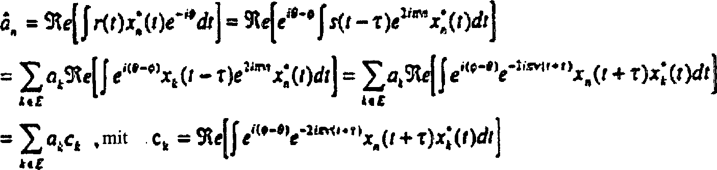
Das demodulierte Signal wird demnach endlich wie folgt geschrieben:The demodulated signal is finally written as follows:
![]()
![]()
Der zweite Term stellt dabei die Interferenz zwischen den Symbolen (IES) dar. Betrachtet man die Daten ak als unabhängige aleatorische Variablen der Varianz σ2, so lautet die Varianz I der IES:The second term represents the interference between the symbols (IES). If the data a k are considered as independent aleatory variables of the variance σ 2 , the variance I of the IES is:
![]()
![]()
Die Koeffizienten ck sind aber die Koeffizienten der Zerlegung der Einheitsnorm-Funktion ei(ϕ–θ)e–2iπν(l+τ)xa(l + τ) über die Hilbert'sche Basis der Funktionen xk(t). Es gilt demnach:However, the coefficients c k are the coefficients of the decomposition of the standard function e i (ϕ – θ) e –2iπν (l + τ) x a (l + τ) over the Hilbert basis of the functions x k (t). The following therefore applies:
![]()
![]()
Anders
ausgedrückt,
ist die Varianz des empfangenen Signals konstant und verteilt sich
zwischen dem „nützlichen" Signal cnan und dem Zwischensymbol
mit der Varianz I = (l – ca 2)2.
Die Berechnung des Koeffizienten cn ergibt: 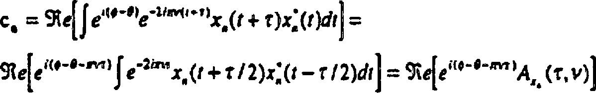
![]()
![]()
Es gilt zuletzt:It last applies:
![]()
![]()
Es
wird angenommen, dass die Demodulationsphase ϕ in der Form ϕopt + Δϕ dargestellt
wird, wobei ϕopt die Demodulationsphase
ist, die das IES minimiert, d. h., die cn maximiert,
oder:
Die Varianz der IES ist dann einfach gegeben durch:The The variance of the IES is then simply given by:
![]()
![]()
Wenn
die Prototypfunktion gerade ist (was dem Falle der im Haupttext
beschriebenen Methode der Konstruktion Hilbert'scher Basen entspricht), so ist die
Mehrdeutigkeitsfunktion reell und es gilt:
Dies
ist ein bemerkenswertes Ergebnis, da es zeigt, dass die Empfindlichkeit
einer jeden Mehrfachträgermodulation
gegenüber
Verzögerung
und Doppler nur von der Mehrdeutigkeitsfunktion ihrer Prototypfunktion
abhängig
ist. Es wird im Nachhinein als genormte Zwischensymbolfunktion (wobei
dieser Ausdruck in vereinfachender Form zur Bezeichnung der Zwischensymbol
Interferenzfunktion genutzt wird), die Funktion![]()
![]()
3. Vergleichende Analyse verschiedener Arten von OFDM3. Comparative Analysis of different types of OFDM
3.1. Theoretische Grenzen3.1. Theoretical limits
Es
werden nun die Eigenschaften der normierten Zwischensymbolfunktion
betrachtet. Es wird bemerkt, dass die Empfindlichkeit einer Mehrfachträgermodulation
direkt mit dem Verhalten der Mehrdeutigkeitsfunktion der entsprechenden
Prototypfunktion in der Nähe
von (0, 0) zusammenhängt.
Das sich ergebende Problem weist eine große Ähnlichkeit mit den Unsicherheitsproblemen
auf, die auf dem Gebiet der Radartechnik auftreten. Man kann demnach
auf die vielfache entsprechende Fachliteratur Bezug nehmen (s. zum
Beispiel [22]). Man kann, ohne Verlust an Allgemeinheit, die Funktion
x(t) durch eine geeignete Verschiebung nach Zeit und Frequenz wählen, so
dass die Zeitpunkte der Ordnung eins den Wert Null haben, oder:
Unter diesen Bedingungen ist es leicht nachzuweisen, dass die partiellen Ableitungen erster Ordnung null werden:Under These conditions make it easy to demonstrate that the partial First order derivatives become zero:

Das Verhalten der Mehrdeutigkeitsfunktion um (0, 0) lässt sich aus den partiellen Ableitungen zweiter Ordnung charakterisieren:The Behavior of the ambiguity function around (0, 0) can be characterize from the partial derivatives of the second order:

Es wird angenommen, dass:It it is believed that:

Betrachten
wir nun die Taylor-Young-Entwicklung der Mehrdeutigkeitsfunktion
bei (0, 0):
Daraus
leitet sich die Taylor-Young-Entwicklung der Varianz des Zwischensymbols
ab
Daraus ergibt sich, dass die Zwischensymbolfunktion ls am Ursprung einen tangierenden Kegel mit der folgenden Gleichung annimmt:from that it follows that the intermediate symbol function ls unites at the origin tangent cone with the following equation:
![]()
![]()
Der
Schnitt dieses Kegels mit der Ebene z = 1 (maximales Zwischensymbol)
begrenzt eine Oberfläche mit
elliptischem Umfang, dessen Fläche ξ als ein
Maß der
Empfindlichkeit gegenüber
Verzögerung
und Doppler gelten kann. Wenn μx null ist, so sind die Symmetrieachsen der
Ellipse jeweils die Zeit- und Frequenzachse. Die Ellipse erstreckt
sich zwischen ±1/2πΔf auf der
Zeitachse und ±1/2πΔf auf der
Frequenzachse. Es gilt demnach:
Aufgrund der Heisenberg'schen Unschärferelation, kann ξ nicht größer als die Einheit sein. Dieses Ergebnis wird verallgemeinert, wenn μx nicht Null ist. Betrachten wir nun die Funktion y(t), die durch Multiplikation der Funktion x(t) mit einem Wobbeln erhalten wird:Due to the Heisenberg uncertainty principle, ξ cannot be larger than the unit. This result is generalized when μ x is not zero. Let us now consider the function y (t), which is obtained by multiplying the function x (t) by a wobble:
![]()
![]()
Man kann demnach schreiben:you can therefore write:

Es ist demnach immer möglich, μy durch geeignete Wahl von β zu annullieren. Dabei verursacht die Multiplikation durch ein Wobbeln lediglich einen Wechsel der Achsen der assoziierten Mehrdeutigkeitsfunktion, mit Erhaltung der Flächen. Daraus ergibt sich, dass der Parameter ξ stets zwischen 0 und 1 liegt.It is therefore always possible to cancel μ y by choosing β appropriately. The multiplication by wobbling only causes a change of the axes of the associated ambiguity function, with preservation of the areas. This means that the parameter ξ is always between 0 and 1.
Dieses Ergebnis ist von außerordentlicher Wichtigkeit, da es den Vergleich der Leistungen aller MCM in dispergierenden Kanälen, ausgehend von einem einzigen Parameter, ermöglicht. Man stellt demnach fest, dass diese Leistungen nur von der Konzentration der assoziierten Prototypfunktion abhängig sind. Das Optimum wird virtuell durch die Gauss'sche Funktion erzielt, aber dieses Optimum ist unerreichbar, da die Gauss'schen Funktionen die Konstruktion einer Hilbert'schen Basis nicht ermöglichen.This The result is extraordinary Importance as it compares the performance of all MCMs in dispersing channels, starting from a single parameter. So you ask notes that these accomplishments depend only on the concentration of the associated Prototype function dependent are. The optimum is achieved virtually by the Gaussian function, but this optimum is unreachable because the Gaussian Functions that do not allow the construction of a Hilbert base.
3.2. Sonderfall der OFDM mit Schutzintervall3.2. Special case of the OFDM with guard interval
Die auf der Grundlage eines Gitters der Dichte 1 konstruierten OFDM-Modulationen bilden einen entarteten Fall: aufgrund des Satzes von Balian-Low-Coifman-Semmes, ist der Parameter ξ in diesem Fall Null. Dieses Ergebnis ist allerdings vollkommen allgemein und gilt unabhängig von der Struktur des Baryzentrumgitters der Basisfunktionen. Man kann nämlich immer, ausgehend von den zeitlichen Wobbeloperatoren, von den Fouriertransformierten und von den Ähnlichkeitstransformationen, bei einer beliebigen orthogonalen Struktur ankommen, für welche der Satz von Balian-Low-Coifman-Semmes gilt. Diese drei Operatoren bewirken aber lediglich Achsenwechsel der Mehrdeutigkeitsfunktion, wobei die Flächen erhalten werden. Daraus folgt, dass der Parameter ξ für alle Modulationen dieser Art null ist.The form OFDM modulations constructed on the basis of a grid of density 1 a degenerate case: based on the theorem of Balian-Low-Coifman-Semmes, is the parameter ξ in in this case zero. However, this result is completely general and applies independently on the structure of the barycenter lattice of the basic functions. you can namely always, starting from the temporal wobble operators, from the Fourier transforms and from the similarity transformations, arrive at any orthogonal structure for which the Balian-Low-Coifman-Semmes theorem applies. These three operators cause only change of axis of the ambiguity function, being the faces be preserved. It follows that the parameter ξ for all modulations of this kind is zero.
Die OFDM/QAM-Modulation entgeht dieser Regel nicht. In diesem Falle ist der Parameter Δf unendlich, was eine starke Empfindlichkeit gegenüber zeitlicher Verschiebungen zur Folge hat (die Zwischensymbolfunktion weist eine vertikale Tangente nach der Zeitachse auf). Dafür verfügt die OFDM/QAM über einen „Joker", über den keine andere Art von OFDM verfügt, und der darin besteht, dass man im Inneren eines durch ein Schutzintervall verlängerten Symbols eine unendliche Menge von verschobenen Versionen des Ausgangssymbols findet. Diese einzigartige Eigenschaft macht die OFDM/QAM zu einer echten Singularität innerhalb der Menge der komplexen MCM.The OFDM / QAM modulation does not escape this rule. In this case is the parameter Δf infinite, which is a strong sensitivity to temporal shifts (the intermediate symbol function has a vertical tangent according to the timeline). Therefore has the OFDM / QAM about a "joker" about which has no other type of OFDM and that is that one inside by a guard interval extended Symbol an infinite amount of shifted versions of the source symbol place. This unique property makes the OFDM / QAM one real singularity within the set of complex MCM.
Das
Schutzintervall bildet einen Nicht-Zwischensymbol-Bereich, welches
die künstliche
Umwandlung des der Zwischensymbolfunktion tangentialen Kegels (der
in diesem Falle vollkommen zeitlich abgeflacht ist) in einem Prisma,
deren Schnitt mit der Ebene z = 1 ein nicht entartetes Rechteck
ist, d. h., dessen Fläche
nicht null ist. Um die Wirkung des Schutzintervalls besser zu verstehen,
wird auf

Es wird sofort nachgewiesen, dass Δt2 = τ0 2/12 ist. Demzufolge ist der Schnitt des die Zwischensymbolfunktion tangierenden Prismas mit der Ebene z = 1 in Frequenzrichtung auf ±√3/πτ0 begrenzt. Nehmen wir an, dass der Zwischensymbolpegel auf –10 dB beschränkt werden soll. Für eine optimale Modulation mit ξ = 1, liegt die Fläche des Zwischensymbolbereiches, die kleiner als –10 dB ist, in der Größenordnung von 0.1. Um ein gleichwertiges Ergebnis mit einer OFDM-Modulation mit Schutzintervall zu erzielen, muss das Schutzintervall Δτ so sein, dass Δτ × (2,√3/πτ0)/√10 ≈ 0.1, oder Δτ ≈ 0.287 τ0. Dieser Wert ist sehr hoch und zeigt gut den erforderlichen Preis, um ein OFDM-System unter ungünstigen Verzögerungs- und Dopplerbedingungen zu betreiben.It is immediately demonstrated that At is 2 = τ 0 2/12. Accordingly, the intersection of the prism tangent to the intermediate symbol function with the plane z = 1 in the frequency direction is limited to ± √3 / πτ 0 . Let us assume that the intermediate symbol level should be limited to –10 dB. For an optimal modulation with ξ = 1, the area of the intermediate symbol area, which is smaller than -10 dB, is of the order of 0.1. In order to achieve an equivalent result with an OFDM modulation with protection interval, the protection interval Δτ must be such that Δτ × (2, √3 / πτ 0 ) / √10 ≈ 0.1, or Δτ ≈ 0.287 τ 0 . This value is very high and shows the price required to operate an OFDM system under unfavorable delay and Doppler conditions.
ANHANG 3APPENDIX 3
1. Einleitung1 Introduction
In diesem Anhang findet man alle Nachweise für die Existenz von Zeit-Frequenz-Transformierten, die symmetrisch gegenüber den Zeit-Frequenz-Achsen sind. In diesem Sinne zeigen diese Transformierten eine starke Ähnlichkeit zur Gabortransformierten, die durch perfekte Isotropie in alle Richtungen der Zeit-Frequenz-Ebene gekennzeichnet ist. Obwohl die Isotropie dieser neuen Transformierten nur annähernd ist, nennen wir sie isotrop, der Einfachheit halber. Der wesentliche Unterschied im Vergleich zur Gabortransformierten ist, dass diese Transformierten streng orthogonal sind, so dass man ihre Anwendung auf den Bereich des digitalen Sendens ins Auge fassen kann. In der Tat garantiert die Orthogonalität der Transformierten die Erhaltung der euklidischen Metriken, was eine wesentliche Eigenschaft in einem Kanal mit additivem Gauss'schen Rauschen ist.In This appendix contains all the evidence for the existence of time-frequency transforms, the symmetrical opposite the time-frequency axes. In this sense, they show transformed a strong resemblance to the Gabor transform, which is perfect in all directions through perfect isotropy the time-frequency level is marked. Although the isotropy of this new transform only approximately we call it isotropic, for the sake of simplicity. The essential The difference compared to the Gabor transform is that this Transforms are strictly orthogonal, so you can apply them can focus on the field of digital broadcasting. In the Tat guarantees orthogonality of the transformed the preservation of Euclidean metrics what is an essential property in a channel with additive Gaussian noise.
Die sich aus diesem Ansatz ergebenden Modulationssysteme verwenden isotrope orthogonale Transformationsalgorithmen (Isotropic Orthogonal Transform Algorithms), so dass wir sie „IOTA" Modulationssysteme genannt haben.The Modulation systems resulting from this approach use isotropic ones orthogonal transformation algorithms (Isotropic Orthogonal Transform Algorithms) so we use "IOTA" modulation systems have mentioned.
2. Mehrdeutigkeitsfunktion2. Ambiguity function
Die Untersuchungen der Mehrdeutigkeitsfunktion wurden in der Vergangenheit im Wesentlichen durch die Entwicklung der Radartechnik bedingt. In diesem Kapitel werden die Haupteigenschaften dieser Funktion wieder aufgerufen. Es werden außerdem verschiedene Operatoren beschrieben, die auf diese Funktion wirken.The Studies of the ambiguity function have been done in the past essentially due to the development of radar technology. In this chapter the main features of this feature are again called. It will also describes various operators that act on this function.
2.1 Erinnerungen an die Mehrdeutigkeitsfunktion2.1 memories of the ambiguity
2.1.1 Definitionen2.1.1 Definitions
Sei eine Funktion x(t) und ihre Fouriertransformierte X(f). Man kann dieser Funktion ihre Zeit- und Frequenzprodukte zuordnen, die jeweils definiert sind durch:Be a function x (t) and its Fourier transform X (f). One can assign their time and frequency products to this function, each are defined by:

Die Wigner-Ville-Transformierte und die Mehrdeutigkeitsfunktion von x sind dann gegeben von:The Wigner-Ville transform and the ambiguity function of x are then given by:

2.1.2. Symmetrieeigenschaften der Mehrdeutigkeitsfunktion2.1.2. symmetry properties the ambiguity function
Sei
eine Funktion x(t). Es werden jeweils mit x– und
![]()
![]()
Es
gelten dann die Beziehungen: ![]()
![]()
![]()
![]()
Daraus folgt insbesondere, dass wenn eine Funktion x gerade ist, d. h., x = x–, ihre Mehrdeutigkeitsfunktion reell ist. Andererseits wird auf die folgende Beziehung hingewiesen:It follows in particular that if a function x is even, ie x = x - , its ambiguity function is real. On the other hand, the following relationship is pointed out:
![]()
![]()
Durch
Kombination dieser zwei Beziehungen erhält man:
2.1.3. Mehrdeutigkeitsfunktion und Fouriertransformierte2.1.3. ambiguity and Fourier transforms
Die
Definition der Mehrdeutigkeitsfunktion kann folgendermaßen neu
geschrieben werden: ![]()
![]()
2.1.4. Mehrdeutigkeitsfunktion und Zeit-Frequenz-Verschiebung2.1.4. ambiguity and time-frequency shift
Betrachten wir eine verschobene Funktion einer beliebigen Prototypfunktion x(t), nämlich:Consider we shift a function of any prototype function x (t), namely:
![]()
![]()
Die
assoziierte Mehrdeutigkeitsfunktion lässt sich folgendermaßen darstellen: 
![]()
![]()
2.2. Orthogonalität und Mehrdeutigkeitsfunktion2.2. Orthogonality and ambiguity function
2.2.1. Allgemeiner Fall2.2.1. General case
Es werden zwei verschobene Funktionen einer selben Funktion x(t) betrachtet, nämlich:It two shifted functions of the same function x (t) are considered, namely:

Das
Skalarprodukt dieser zwei Funktionen lautet dann: ![]()
![]()
![]()
![]()
3. Hilbert'sche Basen über orthogonale Gitter3. Hilbert bases over orthogonal grid
3.1. Allgemeine Konstruktionsprinzipien3.1. General design principles
Es wird eine Menge von Funktionen {xm,n} betrachtet, die folgendermaßen definiert sind:Consider a set of functions {x m, n } that are defined as follows:
![]()
![]()
Es werden die Bedingungen über x(t) gesucht, damit die Menge {xm,n} eine Hilbert'sche Basis von R bildet. Es wird verlangt, dass x(t) eine gerade Funktion ist, deren Mehrdeutigkeitsfunktion Ax demnach reell ist.The conditions over x (t) are searched so that the set {x m, n } forms a Hilbert basis of R. It is required that x (t) is an even function whose ambiguity function A x is therefore real.
Das Skalarprodukt von xm,n und xm',n' in R lässt sich demnach folgendermaßen ausdrücken:The scalar product of x m, n and x m ', n' in R can therefore be expressed as follows:

Es
sei auf die Kongruenzbeziehung Modulo 2 hingewiesen:
Ist
demnach (m, n) ≠ (m', n') Modulo 2, so ist
das Skalarprodukt null. Das Gitter {xm,n}
lässt sich
demnach in 4 Untergitter aufteilen, die durch folgende Beziehung
charakterisiert sind:
{m gerade, n gerade}, {m gerade, n ungerade},
{m ungerade, n gerade}, {m ungerade, n ungerade}.Accordingly, if (m, n) ≠ (m ', n') modulo 2, the dot product is zero. The grid {x m, n } can therefore be divided into 4 sub-grids, which are characterized by the following relationship:
{m even, n even}, {m even, n odd}, {m odd, n even}, {m odd, n odd}.
Die Orthogonalität zwischen Funktionen aus verschiedenen Untergitter ist demnach automatisch und hängt nicht von den Eigenschaften der Prototypfunktion ab, wenn diese gerade ist.The orthogonality between functions from different sub-grids is therefore automatic and hangs does not depend on the properties of the prototype function if this is straight.
Es
muss nur noch garantiert werden, dass die Funktionen eines selben
Gitters untereinander orthogonal sind. Dazu muss die Mehrdeutigkeitsfunktion
Ax nur der folgenden Beziehung genügen:
Es wird demnach ersichtlich, dass das Problem der Konstruktion Hilbert'scher Basen in HR über ein orthogonales Gitter der Dichte 2 sich auf das Problem der Konstruktion einer geraden Prototypfunktion zurückführen lässt, deren Mehrdeutigkeitsfunktion über ein Gitter der Dichte 1/2 null wird.It can thus be seen that the problem of constructing Hilbert bases in H R over an orthogonal grid of density 2 can be traced back to the problem of constructing a straight prototype function whose ambiguity function becomes zero via a grid of density 1/2.
3.2. Orthogonalisierungsmethoden3.2. Orthogonalisierungsmethoden
3.2.1. Orthogonalisierung nach der Zeit3.2.1. orthogonalization after the time
Definition:Definition:
Sei x(t) eine Funktion einer Fouriertransformierten X(f). Man nennt Ot den Operator der zeitlichen Orthogonalisierung, der x(t) eine Funktion y(t) assoziiert, die durch ihre Fouriertransformierte Y(f) definiert ist:Let x (t) be a function of a Fourier transform X (f). O t is called the operator of temporal orthogonalization, which associates x (t) with a function y (t), which is defined by its Fourier transform Y (f):

Durch
Konstruktion hat man: ![]()
![]()
![]()
![]()
Die Orthogonalisierung erfolgt demnach tatsächlich auf der Zeitachse.The Accordingly, orthogonalization actually takes place on the time axis.
Sei x eine Gauss'sche Funktion und y = Otx. Man betrachte den Ausdruck:Let x be a Gaussian function and y = O t x. Consider the expression:

Da
X eine Gauss'sche
Funktion ist, kann man schreiben:
Durch
umgekehrte Fouriertransformierte erhält man:
Demnach:
Der Operator der zeitlichen Orthogonalisierung Ot orthogonalisiert demnach das gesamte Gitter, mit Ausnahme der Frequenzachse.The operator of the temporal orthogonalization O t therefore orthogonalizes the entire grid, with the exception of the frequency axis.
Theorem 1Theorem 1
Sei
x eine Gauss'sche
Funktion und y = Otx, dann gilt:
3.2.2. Orthogonalisierung nach der Frequenz3.2.2. orthogonalization according to the frequency
Definitiondefinition
Sei eine Funktion x(t). Man nennt Of den Orthogonalisierungsoperator nach der Frequenz, der x(t) eine Funktion y(t) assoziiert, welche definiert wird durch:Let be a function x (t). O f is called the orthogonalization operator according to frequency, which associates x (t) with a function y (t), which is defined by:

Durch
Konstruktion hat man: ![]()
![]()
![]()
![]()
Die Orthogonalisierung erfolgt demnach tatsächlich auf der Achse der Frequenzen.The Orthogonalization therefore takes place on the axis of the frequencies.
Sei x eine Gauss'sche Funktion und z = Oty, wobei y = Otx. Man betrachte den Ausdruck:Let x be a Gaussian function and z = O t y, where y = O t x. Consider the expression:

Demnach
kann man schreiben:
![]()
![]()
Durch Fouriertransformierte erhält man:By Fourier transform you:
![]()
![]()
Es
gilt aber:
So annulliert sich die Mehrdeutigkeitsfunktion von z außerhalb (0, 0) für alle Mehrfache von 2τ0 und von 2ν0, d. h., man erhält ein Gitter der Dichte 1/2.Thus the ambiguity function of z outside (0, 0) is canceled for all multiples of 2τ 0 and 2ν 0 , that is, a grating of density 1/2 is obtained.
Theorem 2Theorem 2
Sei
x eine Gauss'sche
Funktion und z = OfOtx,
dann gilt:
3.3. Der Orthogonalisierungsoperator O3.3. The orthogonalization operator O
Anbetracht dessen, was oben erläutert wurde, wird eindeutig, dass es eine Zeit-Frequenz-Skala gibt, welche die Schrift der Gleichungen symmetrisiert: dazu muss lediglich τ0 = ν0 = 1/√2 gewählt werden. Die Skalen werden demnach entsprechend erneut normiert, ohne dass dies der Allgemeinheit der Beweise schadet.In view of what has been explained above, it becomes clear that there is a time-frequency scale that symmetrizes the writing of the equations: all that needs to be chosen is τ 0 = ν 0 = 1 / √2. Accordingly, the scales are standardized again without harming the generality of the evidence.
3.3.1. Definition3.3.1. definition
Sei O der Orthogonalisierungsoperator, der einer Funktion x die Funktion y assoziiert, die durch den folgenden Ausdruck definiert ist:Be O the orthogonalization operator, that of a function x the function y associated, which is defined by the following expression:

Ferner wird nachfolgend der Operator der Fouriertransformierten F genannt.Further The operator of the Fourier transform F is called below.
3.3.2. Idempotenz des Operators O3.3.2. Idempotency of Operator O
Sei z = Oy und y = Ox. Man kann schreiben: Be z = Oy and y = Ox. You can write:

Es gilt demnach OOx = Ox, was die Idempotenz des Operators O beweist.It therefore OOx = Ox, which proves the idempotency of the operator O.
In derselben Weise ist der duale Operator F–1OF ebenfalls idempotent, da F–1OFF–1OF = F–1OOF = F–1OF.In the same way, the dual operator F -1 OF is also idempotent since F -1 OFF -1 OF = F -1 OOF = F -1 OF.
3.3.3. Lemma 13.3.3. Lemma 1
Sei P eine periodische Funktion mit der Periode 1/√2 und D eine Verteilung der Form:Be P is a periodic function with the period 1 / √2 and D is a distribution of the Shape:
![]()
![]()
Sei x eine beliebige Funktion:Be x any function:

Lemma 1Lemma 1
Sei
P eine periodische Funktion mit der Periode 1/√2 und D eine Verteilung der
Form:![]()
![]()
3.3.4. Lemma 23.3.4. Lemma 2
Sei
die Funktion yα,
definiert durch yα = D*xα, wobei![]()
![]()
![]()
![]()
![]()
![]()
Sei zα = Oyα. Es gilt:Let z α = Oy α . The following applies:

Die Summe unter der Wurzel kann man folgendermaßen schreiben:The Sum under the root can be written as follows:
![]()
![]()
Oder,
durch Anwendung des im Anhang angegebenen Ergebnisses: ![]()
![]()
![]()
![]()
Man
kann auch schreiben: ![]()
![]()
![]()
![]()
Demnach
gilt:

Sei![]()
![]()
Zuletzt
kann man schreiben:
Lemma 2Lemma 2
Sei
x eine Gauss'sche
Funktion und D eine Verteilung der Art ![]()
![]()
3.3.5. Kommutativität der Operatoren O und F–1OF3.3.5. Commutativity of the operators O and F –1 OF
Es
soll nun bewiesen werden, dass die Operatoren O und F–1OF
kommutativ sind, wenn sie auf eine Gauss'sche Funktion angewandt werden: Sei![]()
![]()
In anbetracht der periodischen Eigenschaft von Pα, kann man seine Fouriertransformierte Dα wie folgt schreiben:Considering the periodic property of P α , one can write his Fourier transform D α as follows:
![]()
![]()
Betrachten
wir nun die Funktion zα, die das Ergebnis der
Orthogonalisierung von yα durch 0 ist, wobei yα das
Ergebnis der Orthogonalisierung von xα durch
F–1OF
ist. Dann gilt:
Ferner bemerkt man, dass:
- – für jede gerade reelle Funktion x, gilt F–1x = Fx
- – ist c eine positive Konstante, so gilt O[cx] = Ox
- – für jede gerade reelle Funktion x(u) sind Ox, Fx und F–1x gerade reelle Funktionen
- - for every real function x, F –1 x = Fx
- - if c is a positive constant, then O [cx] = Ox
- - for every just real function x (u), Ox, Fx and F –1 x are just real functions
In
anbetracht dieser Bemerkungen kann man schreiben:
Die
Anwendung des Lemmas 2 ergibt:
In
gleicher Weise kann man schreiben:
Die
Anwendung des Lemmas 2 ergibt:
Jedoch
ergibt die Anwendung des Lemmas 1:
Demnach
ergibt sich:
Jedoch besitzen OF–1OFxα und F–1OFOxα beide Einheitsnormen und sind somit gleich.However, OF -1 OFx α and F -1 OFOx α both have uniform standards and are therefore the same.
Theorem 3Theorem 3
Für jede Gauss'sche Funktion x sind
die Operatoren O und F–1OF kommutativ, oder:
Korollar
1 ![]()
![]()
Beweis:
Bemerkenswerter SonderfallNotable special case
Diese
besondere Funktion verleiht der Zeit- sowie der Frequenzachse eine
perfekte Symmetrie und bildet somit die Prototypfunktion der IOTA-Transformierten (Isotropic
Orthogonal Transform Algorithm). Diese besondere Funktion wird mit ![]()
![]()
Korollar 2Corollary 2
Sei x eine Gauss'sche Funktion und z = OF–1OFx, dann gilt Oz = zLet x be a Gaussian function and z = OF –1 OFx, then Oz = z
Beweis:
Korollar 3Corollary 3
Sei x eine Gauss'sche Funktion und z = OF–1OFx, dann gilt F–1OFz = zLet x be a Gaussian function and z = OF –1 OFx, then F –1 OFz = z
Beweis:
3.3.6. Mehrdeutigkeitsfunktion der Funktionen zα 3.3.6. Ambiguity function of the functions z α
Betrachtet
man den Theorem 2 mit der Normierung τ0 = τ0 =
1/√2.
Es gilt:
Theorem 2 kann demnach in folgender Weise neu ausgedrückt werden:theorem 2 can therefore be re-expressed in the following way:
Theorem 4Theorem 4
Sei
x eine Gauss'sche
Funktion und z = F–1FOx. Dann gilt:
4. Verallgemeinerung auf beliebige Gitter4. Generalization on any grid
Bisher wurden auf einem orthogonalen Gitter der Dichte 2 aufgebaute Hilbert'sche Basen betrachtet. In diesem Kapitel werden Hilbert'sche Basen betrachtet, die auf einem beliebigen Gitter der Dichte 2 aufgebaut sind.So far were examined on an orthogonal grid with density 2 Hilbert bases. In In this chapter Hilbert's Consider bases built on any density 2 grid.
4.1. Allgemeine Konstruktionsprinzipien4.1. General design principles
In ähnlicher Weise wie für orthogonale Gitter bewiesen, wird in diesem Absatz die Konstruktion einer Hilbert'schen Basis über einem beliebigen Gitter der Dichte 2 bewiesen, ausgehend von einer Prototypfunktion, deren Mehrdeutigkeitsfunktion über einem Gitter der Dichte 1/2 null wird.More like that Way like for The construction is proved in this paragraph a Hilbertian Base over proved any grid of density 2, starting from one Prototype function, its ambiguity function over a grid of density 1/2 becomes zero.
Sei
ein allgemeines Gitter der Dichte 2, das auf der Grundlage von Basisvektoren
(τ1, ν1) und (τ2, ν2) erzeugt wird, mit |ν1τ2 – ν2τ1|
= 1/2. Es wird als Konvention die Reihenfolge der Basisvektoren
so gewählt,
dass ν2τ1 – ν1τ2 =
1/2. Es wird eine Funktion x(t) betrachtet, so dass:
![]()
![]()
Es
werde das Skalarprodukt <xm,n|xm,n> berechnet, d. h.: ![]()
![]()
Es gilt aber: ν2τ1 – ν1τ2 = 1/2However, the following applies: ν 2 τ 1 - ν 1 τ 2 = 1/2
Setzt
man: ![]()
![]()
Sei: φm,n = (m + n)π/2 – ψm,n Dann wird das Skalarprodukt <xm,n|xm',n'>R endlich:Let: φ m, n = (m + n) π / 2 - ψ m, n Then the scalar product <x m, n | x m ', n' > R finally:
![]()
![]()
Da die Mehrdeutigkeitsfunktion von x reell ist, ist ihr Koeffizient von Interesse. Man findet denselben Phasenterm wie im Falle eines orthogonalen Gitters wieder. Demnach, wenn (m, n) ≠ (m', n') Modulo 2, ist das Skalarprodukt null. Andernfalls ist es ebenfalls null aufgrund der bezüglich der Mehrdeutigkeitsfunktion von x getroffenen Annahme.There the ambiguity function of x is real is its coefficient of interest. One finds the same phase term as in the case of one orthogonal grid again. Hence, if (m, n) ≠ (m ', n') modulo 2, is the dot product zero. Otherwise, it is also zero due to the Ambiguity function of x assumption made.
Somit verfügt man über eine allgemeine Methode zum Konstruieren von Hilbert'schen Basen über beliebige Gitter in der Zeit-Frequenz-Ebene. Es bleiben somit Prototypfunktionen zu konstruieren, deren Mehrdeutigkeitsfunktion die geforderten Eigenschaften aufweist.Consequently has one over a general method for constructing Hilbert bases over any Grid in the time-frequency plane. Prototype functions remain to construct, the ambiguity function the required properties having.
4.2. Koordinatenwechsel in der Zeit-Frequenz-Ebene4.2. coordinate change in the time-frequency level
Wir haben bisher Operatoren angetroffen, deren Aktion ohne Schwierigkeiten in der Zeit-Frequenz-Ebene gedeutet werden konnte, so beispielsweise die Orthogonalisierungsoperatoren, die Annullierungspunkte der Mehrdeutigkeitsfunktion über ein orthogonales Gitter der Dichte 1/2 erzeugen. Nachfolgend werden neue Operatoren betrachtet, die Koordinatenwechsel in der Zeit-Frequenz-Ebene verursachen. Mit diesen Operatoren lässt sich eine Prototypfunktion, deren Mehrdeutigkeitsfunktion über ein orthogonales Gitter der Dichte 1/2 null wird, in eine Prototypfunktion umwandeln, deren Mehrdeutigkeitsfunktion über ein beliebiges Gitter der Dichte 1/2 null wird.We have encountered operators so far, their action without difficulty could be interpreted in the time-frequency level, for example the orthogonalization operators, the cancellation points of the ambiguity function over one create an orthogonal grid of density 1/2. Be below considered new operators that change coordinates in the time-frequency plane cause. With these operators, a prototype function can be whose ambiguity function over an orthogonal grid of density 1/2 becomes a prototype function convert whose ambiguity function over any grid of Density 1/2 becomes zero.
Sei
ein Operator T, der einer Funktion die Funktion y = Tx assoziiert,
so dass:
Der Operator T bewirkt demnach einen Koordinatenwechsel in der durch die Matrix MT charakterisierten Zeit-Frequenz-Ebene.The operator T accordingly effects a change of coordinates in the time-frequency plane characterized by the matrix M T.
4.3. Basisoperatoren4.3. Basic operators
4.3.1. Fouriertransformierten-Operator4.3.1. Fourier transform operator
Es
wurde oben gezeigt, dass wenn X die Transformierte von x ist, d.
h., X = Fx, die folgende Beziehung gilt:
Die entsprechende charakteristische Matrix ist demnach:The the corresponding characteristic matrix is therefore:
![]()
![]()
Diese Matrix entspricht einer Drehung um –π/2 in der Zeit-Frequenz-Ebene.This Matrix corresponds to a rotation of –π / 2 in the time-frequency plane.
4.3.2. Phasenverschiebungsoperator4.3.2. Phase shift operator
Angenommen
Pθ sei
der Phasenverschiebungsoperator, der einer Funktion x die Funktion
y assoziiert, so dass:
Es
gilt eindeutig:
4.3.3. Ähnlichkeits-Transformationsoperator4.3.3. Similarity transformation operator
Der Ähnlichkeits-Transformationsoperator
Hγ ist
der Operator, der einer Funktion x(t) die Funktion y(t) assoziiert,
die folgendermaßen
definiert ist: ![]()
![]()
Es gilt somit:It the following therefore applies:
![]()
![]()
Sei u = t/γ. Wenn γ positiv ist, so gilt:Be u = t / γ. If γ positive is, the following applies:
![]()
![]()
Wenn γ negativ ist, so gilt:If γ is negative is, the following applies:
![]()
![]()
In
beiden Fällen
gilt Aγ =
(τ, ν) = Ax(τ/γ, γν) oder:
Demnach gilt:Therefore applies:
![]()
![]()
4.3.4. Wobbeloperatoren4.3.4. Wobbeloperatoren
Eine einfache Methode zum Ändern der Mehrdeutigkeitsfunktion einer Funktion besteht darin, sie mit einem Wobbelsignal zu multiplizieren. Man nennt Wβ den zeitlichen Wobbeloperator, der einer Funktion x(t) die Funktion y(t) assoziiert, die folgendermaßen definiert ist:A simple way to change a function's ambiguity function is to multiply it by a wobble signal. W β is called the temporal wobble operator, which associates the function y (t) with a function x (t), which is defined as follows:
![]()
![]()
Es
gilt dann: ![]()
![]()
![]()
![]()
![]()
![]()
4.4. Gruppe der Zeit-Frequenz-Operatoren4.4. Group of time-frequency operators
Es
werden alle Operatoren betrachtet, die durch eine endliche Vereinigung
der oben beschriebenen Basisoperatoren erzeugt werden können. Es
sei zuerst darauf hingewiesen, dass wenn y = Tx = T1 T2 ... Tn x, dann
gilt ebenfalls:
Es ist eindeutig, dass diese Menge, versehen mit dem als Vereinigung der Operatoren definierten Produkt, eine Gruppenstruktur aufweist.It is clear that this set, provided with that as a union of the operators defined product, has a group structure.
4.4.1. Grundregeln für das Multiplizieren von Operatoren4.4.1. Basic rules for multiplying of operators
Das
Multiplizieren von Operatoren richtet sich nach den folgenden Regeln:
Andererseits können F2 und Pθ mit allen anderen Operatoren kommutieren. Es werden die folgenden Beziehungen notiert:On the other hand, F 2 and P θ can commute with all other operators. The following relationships are noted:
![]()
![]()
Sei u' = u/γ. Wenn γ positiv ist:Be u '= u / γ. If γ positive is:
![]()
![]()
Wenn γ negativ ist:If γ is negative is:
![]()
![]()
In beiden Fällen gilt demnach HγF = FH1/γ.In both cases, H γ F = FH 1 / γ applies.
In
gleicher Weise hat man: ![]()
![]()
![]()
![]()
4.4.2. Ausweitung des „Chirp Transform Algorithm"4.4.2. Expansion of the “Chirp Transform algorithm "
Die oben beschriebenen Regeln ermöglichen das Kommutieren aller Operatoren untereinander, mit Ausnahme der Fouriertransformierten und des Wobbeloperators. Die Regeln zum Kommutieren dieser Operatoren sind komplexer und lassen sich auf der Grundalge des „Chirp Transform" Algorithmus extrapolieren.The Allow rules described above the commutation of all operators with the exception of the Fourier transform and the wobble operator. The rules for commutating these operators are more complex and can be based on algae the "Chirp Transform "algorithm extrapolate.
Es
wird hier eine Beziehung betrachtet, welche die Operatoren F, W
und H verbindet. Sei δt(u)= δ(u – t). Da
die betrachteten Operatoren linear sind, lassen sich ihre Eigenschaften
analysieren, indem man ihre Wirkung auf die Verteilungen δt auf
der Grundlage der folgenden Beziehung analysiert:
Es
gilt: 
![]()
![]()
4.4.3. Kanonische Zerlegung4.4.3. Canonical decomposition
Sei
ein Element der Menge der oben definierten Operatoren. Wenn dieses
Element keinen Operator F umfasst, so kann man unter Verwendung
der in 4.4.1. gegebenen Regeln diesen Operator auf die Form reduzieren:
Umfasst
dieses Element nur einen einzigen Operator F, so lässt er sich,
unter Anwendung derselben Regeln, auf die Form reduzieren:
Umfasst
dieses Element mindestens zwei Operatoren F, so lässt es sich
auf die Form reduzieren:
Durch Anwendung der in 4.4.2. gegebenen Regel, lassen sich die Operatoren F iterativ eliminieren, und man erhält zuletzt eine Darstellung, die nur einen einzigen Operator aufweist. Zusammenfassend, lassen sich alle Elemente der Gruppe unter einer der oben angegebenen Formen darstellen.By Application of the in 4.4.2. Given the rule, the operators Eliminate it iteratively, and finally you get a representation which has only one operator. In summary, can all elements of the group under one of the forms specified above represent.
Sei T ein Element der Gruppe, die unter der ersten Art von Darstellung geschrieben wird. Ihre charakteristische Matrix ist:Be T is an element of the group under the first type of representation is written. Their characteristic matrix is:
![]()
![]()
Sei T ein Element der Gruppe, die unter der zweiten Darstellungsform geschrieben wird. So ist ihre charakteristische Matrix:Be T is an element of the group under the second form of presentation is written. So their characteristic matrix is:
![]()
![]()
Sei umgekehrt eine beliebige Matrix MT mit Einheitsdeterminante. Man kann ihr einen Operator assoziieren, der unter seiner kanonischen Darstellung beschrieben wird:Conversely, be an arbitrary matrix M T with a unit determinant. You can associate it with an operator, which is described under its canonical representation:
![]()
![]()
Wenn c = 0, so kann man dieser Matrix einen Operator der ersten Art zuordnen, wobei:If c = 0, you can assign an operator of the first kind to this matrix, in which:
![]()
![]()
Wenn c ≠ 0, so kann man dieser Matrix einen Operator der zweiten Art zuordnen, wobei:If c ≠ 0, see above you can assign an operator of the second kind to this matrix, in which:

Es sei darauf hingewiesen, dass eine vollkommene Ungewissheit bezüglich θ bleibt.It it should be noted that there is complete uncertainty about θ.
4.5. Konstruktion einer Hilbert'schen Basis über ein beliebiges Gitter4.5. Construction of a Hilbert base over one any grid
Die
oben beschriebenen Methoden geben eine allgemeine Methode zum Konstruieren
einer Hilbert'schen
Basis über
ein beliebiges Gitter. Sei ein beliebiges Gitter der Dichte 2, erzeugt
aus Basisvektoren (τ1, ν1) und (τ2, ν2), wobei ν2τ1 – ν1τ2 =
1/2. Man betrachtet eine Funktion x(t), für welche gilt:
In der Praxis, kann die Funktion x die Prototypfunktion der OQAM, OMSK oder einer beliebigen Funktion sein, die durch Orthogonalisieren von Gauss'schen Funktionen erzeugt wurden, wie in Kapitel 3 angegeben, und insbesondere die IOTA-Funktion.In In practice, the function x can be the prototype function of the OQAM, OMSK or any function that is orthogonalized von Gaussian Functions were created as specified in Chapter 3, and in particular the IOTA function.
Sei
T ein Operator mit der charakteristischen Matrix MT,
definiert durch: ![]()
![]()
Sei die Menge der Funktionen {ym,n}, die folgendermaßen definiert sind:Let the set of functions {y m, n } be defined as follows:
![]()
![]()
![]()
![]()
Gemäß dem, was in 4.1 nachgewiesen wurde, bildet die Menge der Funktionen {ym,n} eine Hilbert'sche Basis. Man verfügt demnach über eine allgemeine Methode zum Konstruieren von Hilbert'schen Basen über beliebige Gitter in der Zeit-Frequenz-Ebene.According to what was demonstrated in 4.1, the set of functions {y m, n } forms a Hilbert basis. Accordingly, there is a general method for constructing Hilbert bases over any grid in the time-frequency plane.
5. Konstruktion von Hilbert'schen Basen in Quincunx5. Construction of Hilbert bases in Quincunx
Obwohl die oben beschriebene allgemeine Methode von eindeutigem akademischen Interesse ist, haften ihrer praktischen Anwendung bestimmte Schwierigkeiten an. Einerseits sind, im Allgemeinfall, die Demodulationsalgorithmen hochgradig kompliziert aufgrund der schrägen Struktur des Gitters der Basisfunktionen. Andererseits ist die erhaltene Prototypfunktion ebenfalls komplex, was die Komplexität noch erhöht.Even though the general method of clear academic described above It is of interest to have certain difficulties in their practical application on. On the one hand, in general, there are demodulation algorithms highly complicated due to the sloping structure of the grid Basic functions. On the other hand, the prototype function obtained also complex, which increases the complexity.
Man kann demnach die berechtigte Frage stellen, ob diese Verallgemeinerung in irgendeiner Weise von praktischem Interesse ist. Zweck dieses Absatzes ist es, eine vollständige Antwort auf diese Frage zu geben.you can therefore ask the legitimate question whether this generalization is of practical interest in any way. Purpose of this Paragraph is a complete To answer this question.
Sei
die Menge der nach der oben beschriebenen Methode erzeugten Hilbert'schen Basen. Man
sucht innerhalb dieser Menge die Hilbert'schen Basen, deren Prototypfunktion
reell und gerade ist. Die Mehrdeutigkeitsfunktion weist dann die
folgenden Symmetrien auf: ![]()
![]()
![]()
![]()
Es gilt demnach Ax(τ, ν) = Ax(–τ, ν) = Ax(τ–, –ν) = Ax(–τ, ν). Diese Symmetrien der Mehrdeutigkeitsfunktion werden nur dann erzielt, wenn das Annullierungsgitter dieser Funktion dieselben Symmetrien aufweist. Diese Bedingungen gelten jedoch nachweislich nur für zwei Arten von Gittern: das orthogonale Gitter, auf dem alle bisher betrachteten Modulationen beruhen, und das Quincunxgitter.A x (τ, ν) = A x (–τ, ν) = A x (τ–, –ν) = A x (–τ, ν). These symmetries of the ambiguity function are only achieved if the cancellation grid of this function has the same symmetries. However, these conditions have been shown to apply only to two types of grids: the orthogonal grid on which all modulations considered so far are based and the quincunx grid.
Das orthogonale Gitter wird von den Basisvektoren (τ1, ν1) = (1/√2,0) und (τ2, ν2) = (0,1/√2) erzeugt. Das Quincunxgitter wird von den Vektoren (τ1, ν1) = (1/2, –1/2) und (τ2, ν2) = (1/2, 1/2) erzeugt. Man wechselt von einem Gitter zum anderen durch eine Umdrehung um den Winkel –π/4. Deshalb interessieren wir uns nachfolgend ganz besonders für die Operatoren, die eine Drehung in der Zeit-Frequenz-Ebene durchführen.The orthogonal grid is generated from the base vectors (τ 1 , ν 1 ) = (1 / √2.0) and (τ 2 , ν 2 ) = (0.1 / √2). The quincunx lattice is generated by the vectors (τ 1 , ν 1 ) = (1/2, -1/2) and (τ 2 , ν 2 ) = (1/2, 1/2). One changes from one grating to the other by one turn through the angle –π / 4. Therefore, we are particularly interested in the operators below who perform a rotation in the time-frequency plane.
5.1. Untergruppe der Zeit-Frequenz-Drehungsoperatoren5.1. Sub-group of time-frequency rotation operators
Es sei die Gruppe der Operatoren, deren charakteristische Matrix eine Drehung in der Zeit-Frequenz-Ebene ist:It be the group of operators whose characteristic matrix is one Rotation in the time-frequency plane is:
![]()
![]()
Wir haben bereits gezeigt, dass der Operator der Fouriertransformierten F einer Drehung um den Winkel φ = –π/2, während der Operator F3 = F–1 einer Drehung um den Winkel φ = π/2 entspricht.We have already shown that the operator of the Fourier transform F corresponds to a rotation by the angle φ = −π / 2, while the operator F 3 = F −1 corresponds to a rotation by the angle φ = π / 2.
Sei
ein Operator der Form:
Seine charakteristische Matrix ist:His characteristic matrix is:

Mit
den Annahmen γ = –cos φ und α = β = tgφ, erhält man die
Matrix einer Drehung mit dem Winkel φ. Der Parameter θ bleibt
unbestimmt. Um diese Unbestimmtheit aufzuheben, wird die Forderung
gestellt, dass der Operator die Gauss'sche Funktion![]()

![]()
![]()
![]()
Zuletzt kann man schreiben:Last you can write:
![]()
![]()
Definition:Definition:
Man bezeichnet als Rφ den Operator für Drehungen um den Winkel φ in der Zeit-Frequenz-Ebene, der folgendermaßen definiert wird:R φ is the operator for rotations around the angle φ in the time-frequency plane, which is defined as follows:

Sei
eine reelle Zahl α.
Man definiert ebenfalls die Bruchpotenz des Operators F mit Hilfe
der Gleichung:
Die so definierte Operatorenmenge besitzt eine kommutative Gruppenstruktur, die zur Gruppe der Drehungen der Ebene isomorph ist. Die Exponentennotierung des Operators F erfüllt alle „üblichen" Eigenschaften eines Exponenten.The operator set defined in this way has a commutative group structure, which is isomorphic to the group of rotations of the plane. The exponent listing of the operator F is satisfied all "usual" properties of a Exponent.
5.2. IOTA π/45.2. IOTA π / 4
Sei
eine reelle gerade Prototypfunktion x(t), mit der man eine Hilbert'sche Basis auf dem
orthogonalen Gitter erzeugen kann, und die Funktion y(t), die folgendermaßen definiert
wird:
Die Funktion IOTA π/4 wird definiert durch die Beziehung:The IOTA π / 4 function is defined by the relationship:
![]()
![]()
Diese
Funktion ist gemäß Konstruktion
reell und gerade. Die Mehrdeutigkeitsfunktion dieser Funktion wird
demnach null über
ein Quincunxgitter, dass von den Vektoren (τ1, ν1)
= (1/2, –1/2)
und (τ2, ν2) = (1/2, 1/2) erzeugt wird. In Übereinstimmung
mit 4.1. ergibt sich, dass die Menge der Funktionen {![]()
![]()
![]()
![]()
Durch
Neudefinition der Indizes lässt
sich die Definition dieser Menge folgendermaßen darstellen: ![]()
![]()
6. Anhang6. Appendix
Es sei auf die folgende Identität hingewiesen:It be on the following identity note:

Sei x eine normierte Gauss'sche Funktion, definiert durch:Be x a normalized Gaussian Function defined by:
![]()
![]()
Das Produkt x(u – a)×(u – b) kann somit wie folgt geschrieben werden:The Product x (u - a) × (u - b) can thus be written as follows:
![]()
![]()
Man kann zuletzt schreiben:you can write at last:
![]()
![]()
ANHANG 4APPENDIX 4
1. Vom Kontinuierlichen zum Diskreten1. From the continuous to the discrete
In den zwei vorangegangenen Kapiteln wurden Funktionen aus L2(R) betrachtet.Functions from L 2 (R) were considered in the two previous chapters.
In der Praxis setzt die digitale Verarbeitung den Übergang in den Bereich des Diskreten voraus.In In practice, digital processing makes the transition to the field of Discreet ahead.
1.1 Allgemeines1.1 General
Die in der Praxis verwendeten Signale werden stets als beschränkt angesehen, sowohl in der Zeit als auch nach der Frequenz, obwohl diese Annahme eine bekanntlich theoretische Unmöglichkeit darstellt. Dieses Hindernis lässt sich dennoch umgehen und die Signale können durch eine endliche Menge diskreter Werte durch Anwendung der nachfolgenden Methode dargestellt werden.The signals used in practice are always considered to be limited, both in time and in frequency, although this assumption is a known theoretical impossibility. This obstacle let yourself handle it anyway and the signals can go through a finite set discrete values by using the following method become.
Es
werde angenommen, dass ein beliebiges komplexes Signal x(t) in einem
auf [0, T] zeitlich begrenzten und auf [–W/2, W/2] bezüglich der
Frequenzen begrenzten Raum betrachtet wird. Man beschränkt sich
auf den Fall, in dem das Produkt WT ganz ist. Diesem Signal kann
man einen Vektor
![]()
![]()
Die
Summierung nach dem Index q bewirkt ein zeitliches „Aliasing" und „periodisiert" somit das Signal in
der Zeit, während
die Abtastung das Signal bezüglich
der Frequenzen „periodisiert".
So kann man schreiben:So you can write:

Es sei darauf hingewiesen, dass dieses eindeutig „natürliche" Ergebnis nur um den Preis einer besonderen Auswahl der Modulationsfrequenz erzielt wird, die alle „Aliasing"-Probleme eliminiert. Betrachtet man in ähnlicher Weise eine Verschiebung vom Typ y(t) = x(t – n/W), so kann man schreiben:It it should be noted that this clearly "natural" result only at the price of a special one Selection of the modulation frequency is achieved, which eliminates all "aliasing" problems. Looking at it in a similar way If there is a displacement of the type y (t) = x (t - n / W), one can write:

Ganz allgemein garantiert die Wahl von Abtastungsstrukturen nach Zeit und Frequenz, die jeweils Vielfache von 1/W und von 1/T sind, ein harmonisches „Aliasing" der Signale sowie ein Schreiben im diskreten Bereich, das dem Schreiben im kontinuierlichen Bereich gleichwertig ist.All in general, the choice of sampling structures guarantees by time and frequency, which are multiples of 1 / W and 1 / T, respectively harmonic "aliasing" of the signals as well a letter in the discrete area, the letter in the continuous Area is equivalent.
Sei
zuletzt das Skalarprodukt zweier Vektoren 
-
Sei p = n ÷ q'WT und q = q' – q'' Let p = n ÷ q'WT and q = q '- q''

Es gilt jedochIt applies however

1.2. Die IOTA Transformierte1.2. The IOTA Transform
Es wird hier eine erste Transformierte betrachtet, die sich aus den im Kapitel „der theoretische Ansatz" erzielten Ergebnissen ableitet und auf der IOTA-Funktion basiert.It a first transform is considered here, which results from the in the chapter “the theoretical approach " Derives results and is based on the IOTA function.
1.2.1. Die IOTA-Transformierte im kontinuierlichen Bereich1.2.1. The IOTA transform in the continuous area
Es
wird hier eine „normierte" Transformierte betrachtet,
d. h., eine Transformierte, die auf der Grundlage eines Gitters
des vorher beschriebenen Typs (n/√2, m/√2) konstruiert wurde. Man
kann immer zu dieser Situation zurückkehren, durch vorherige Einwirkung
des geeigneten Ähnlichkeitsoperators.
Sei die Hilbert'sche Basis
{![]()
![]()
![]()
![]()
Es sei darauf hingewiesen, dass man alternativ die nachfolgende Formulierung wählen kann:It it should be noted that you can alternatively use the following wording choose can:

Diese Änderung
entspricht einer möglichen
Vorzeichenumkehr der Basisfunktionen. Die IOTA-Transformierte eines
Signals s(t) der Fouriertransformierten S(f) wird dann durch die
folgenden Beziehungen definiert: 

1.2.2. Die diskrete IOTA-Transformierte1.2.2. The discrete IOTA transform
Es
wird T gleich M√2
und W gleich M√2
gewählt.
Diese Wahl garantiert das Fehlen von „Aliasing"-Problemen. Sei eine Basisfunktion ![]()
![]()
![]()
![]()
![]()
![]()

Sei
ein Skalarprodukt der Art ![]()
![]()
![]()
![]()

In anbetracht dieser Bemerkungen, lässt sich die IOTA-Transformierte wie folgt definieren:In considering these comments, lets the IOTA transform is defined as follows:
Definition der IOTA-TransformiertenDefinition of the IOTA transform
Seien
M und N zwei beliebige ganze Zahlen. Man betrachtet 4MN Vektoren
mit den Dimensionen 2MN, die im Sinne des reellen Skalarprodukts
orthogonal sind und folgendermaßen
definiert werden: ![]()
![]()
Sei ![]()
![]()

Die
Matrix {am,n} ist die IOTA-Transformierte
des Vektors
1.3. Die IOTA p/4 Transformierte1.3. The IOTA p / 4 transform
1.3.1 Die IOTA p/4 Transformierte im kontinuierlichen Bereich1.3.1 The IOTA p / 4 transform in the continuous area
Es wird hier eine „normierte" Transformierte betrachtet, d. h., eine Transformierte, die auf der Grundlage des vorher beschriebenen normalisierten Gitters des Quincunxtyps konstruiert wurde. Man kann immer zu dieser Situation zurückkehren, durch vorherige Einwirkung des geeigneten Ähnlichkeitsoperators.It a "normalized" transform is considered here, d. that is, a transform based on the previously described normalized Quincunx type grid. One can always return to this situation by prior action by the appropriate similarity operator.
Sei
die Hilbert'sche
Basis ![]()
![]()
![]()
![]()
Es
lässt sich
leicht nachweisen, dass die folgende Formulierung alternativ anwendbar
ist: 


1.3.2. Die diskrete IOTA π/4 Transformierte1.3.2. The discrete IOTA π / 4 transform
Es
wird T gleich 2N und W gleich 2M gewählt. Diese Wahl garantiert
das Fehlen von Aliasing"-Problemen.
Sei eine Basisfunktion ![]()
![]()
![]()
![]()
![]()
![]()

Sei
ein Skalarprodukt von der Art ![]()
![]()
![]()
![]()

In anbetracht dieser Bemerkungen, kann man die diskrete IOTA π/4 Transformierte folgendermaßen definieren:In Given these remarks, one can see the discrete IOTA π / 4 transform define as follows:
Definitiondefinition
Seien
M und N zwei beliebige ganze Zahlen. Man betrachtet 8MN Vektoren
mit den Dimensionen 4MN; die im Sinne des Skalarproduktes orthogonal
sind und folgendermaßen
definiert sind: ![]()
![]()
Sei ![]()
![]()

Die
Matrix {am,n} ist die IOTA π/4 Transformierte
des Vektors
2. Die schnellen Demodulationsalgorithmen2. The fast demodulation algorithms
2.1. Demodulation durch schnelle IOTA-Transformierte2.1. Demodulation by fast IOTA transform
Es wird eine Modulation des Typs Mehrträger IOTA betrachtet, charakterisiert durch das gesendete Signal:It a modulation of the type multi-carrier IOTA is considered, characterized by the transmitted signal:
![]()
![]()
Sei ein Sendekanal, charakterisiert durch seine variable Transferfunktion T(f, t). Das empfangene Signal wird folgendermaßen geschrieben:Be a transmission channel characterized by its variable transfer function T (f, t). The received signal is written as follows:
![]()
![]()
Der optimale Demodulator schätzt die Transferfunktion T(f, t) mit Hilfe von Mitteln, die auf dieser Höhe nicht beschrieben sind. Um das eigentliche Signal zu demodulieren, wird örtlich der Kanal mit einem multiplikativen Kanal assimiliert, der durch eine Amplitude und eine Phase charakterisiert wird, die dem Wert von T(f, t) zu dem betrachteten Zeitpunkt und zu der betrachteten Frequenz entsprechen. Um am,n zu schätzen, wird das empfangene Signal demnach dem folgenden Signal assimiliert:The optimal demodulator estimates the transfer function T (f, t) using means that are not described at this level. In order to demodulate the actual signal, the channel is locally assimilated with a multiplicative channel which is characterized by an amplitude and a phase which correspond to the value of T (f, t) at the time and frequency considered. In order to estimate a m, n , the received signal is therefore assimilated to the following signal:
![]()
![]()
Sei:Be:
![]()
![]()
Der Demodulator verrichtet demnach die folgende Verarbeitung:The Demodulator therefore performs the following processing:
![]()
![]()
Im
Falle eines stationären
Kanals mit der Transferfunktion peiθ findet
man offensichtlich:
In der Praxis erfolgt die Verarbeitung digital. Man erhält:In In practice, processing is done digitally. You get:

Sei dann p = k + 2Mr, wobei k von 0 bis 2M – 1 und r von 0 bis N – 1 variiert:Be then p = k + 2Mr, where k varies from 0 to 2M - 1 and r from 0 to N - 1:

Diese Gleichung zeigt, dass man einen schnellen Demodulationsalgorithmus verwenden kann, der die folgenden Verarbeitungsschritte umfasst:
- – Vorfilterung des empfangenen Signals durch die Prototypfunktion,
- – „Aliasing" der gefilterten Wellenform Modulo 2M,
- – FFT mit Dimensionen von 2M komplexen Punkten,
- – Korrektur der Phase θm,n + φm,n,
- – Wahl des reellen Teils.
- - pre-filtering of the received signal by the prototype function,
- - "Aliasing" the filtered Modulo 2M waveform,
- - FFT with dimensions of 2M complex points,
- - correction of the phase θ m, n + φ m, n ,
- - choice of real part.
Dieser Algorithmus ermöglicht somit das globale Berechnen aller Koeffizienten eines gegebenen Indexes n. Die Größenordnung der entsprechenden Komplexität beträgt in etwa das Doppelte derjenigen des für die OFDM verwendeten Algorithmus.This algorithm thus enables the global calculation of all coefficients of a given In dexes n. The magnitude of the corresponding complexity is approximately twice that of the algorithm used for the OFDM.
2.2. Demodulation durch schnelle IOTA π/4 Transformierte2.2. Demodulation by fast IOTA π / 4 transformed
Es
wird eine Modulation des Typs Mehrträger IOTA π/4 betrachtet, charakterisiert
durch die Gleichung des gesendeten Signals: ![]()
![]()
Wie vorher gesehen, führt der Demodulator die folgende Verarbeitung aus:How seen before, leads the demodulator does the following processing:
![]()
![]()
In der Praxis erfolgt die Verarbeitung digital. Man erhält:In In practice, processing is done digitally. You get:

Mit der Annahme p = k + 4Mr, wobei k von 0 bis 4M – 1 und r von 0 bis N – 1 variieren, ergibt sich:With assuming p = k + 4Mr, where k varies from 0 to 4M - 1 and r from 0 to N - 1, surrendered:

Diese Gleichung zeigt, dass man einen schnellen Demodulationsalgorithmus verwenden kann, der die folgenden Verarbeitungsschritte umfasst:
- – Vorfilterung
des empfangenen Signals durch die Prototypfunktion

- – „Aliasing" der gefilterten Wellenform Modulo 4M,
- – FFT mit Dimensionen von 4M komplexen Punkten. In der Praxis, ist es ausreichend, die geraden oder ungeraden Punkte nach der Parität von n zu berechnen. Diese teilweise FFT erfolgt durch Dezimieren der Abtastwerte nach dem Verhältnis 2, nach dem ersten Schmetterlings-Strahlerfeld, was einer einfachen zusätzlichen Vorfilterung entspricht (Summe oder Differenz von Abtastwerten). Man kommt dann auf eine FFT mit den Dimensionen 2M Punkte zurück,
- – Korrektur der Phase θm,n + φm,n,
- – Wahl des reellen Teils.
- - Pre-filtering of the received signal by the prototype function
- - "Aliasing" of the filtered Modulo 4M waveform,
- - FFT with dimensions of 4M complex points. In practice, it is sufficient to calculate the even or odd points according to the parity of n. This partial FFT takes place by decimating the samples according to the ratio 2, after the first butterfly radiator field, which corresponds to a simple additional pre-filtering (sum or difference of samples). You then come back to an FFT with the dimensions 2M points,
- - correction of the phase θ m, n + φ m, n ,
- - choice of real part.
Dieser Algorithmus ermöglicht somit das globale Berechnen aller Koeffizienten eines gegebenen Indexes n. Die Größenordnung der entsprechenden Komplexität beträgt in etwa das Doppelte derjenigen des für die OFDM verwendeten Algorithmus.This Algorithm enables thus the global calculation of all coefficients of a given one Indexes n. The order of magnitude the corresponding complexity is approximately twice that of the algorithm used for the OFDM.
Claims (11)
Applications Claiming Priority (3)
| Application Number | Priority Date | Filing Date | Title |
|---|---|---|---|
| FR9613917 | 1996-11-08 | ||
| FR9613917 | 1996-11-08 | ||
| PCT/FR1997/002013 WO1998021861A1 (en) | 1996-11-08 | 1997-11-07 | Prototype signal construction for multicarrier transmission |
Publications (2)
| Publication Number | Publication Date |
|---|---|
| DE69727505D1 DE69727505D1 (en) | 2004-03-11 |
| DE69727505T2 true DE69727505T2 (en) | 2004-12-16 |
Family
ID=9497636
Family Applications (1)
| Application Number | Title | Priority Date | Filing Date |
|---|---|---|---|
| DE69727505T Expired - Lifetime DE69727505T2 (en) | 1996-11-08 | 1997-11-07 | GENERATION OF PROTOTYPE SIGNALS FOR MULTI-CARRIER TRANSMISSION |
Country Status (7)
| Country | Link |
|---|---|
| US (1) | US6584068B1 (en) |
| EP (1) | EP1013042B1 (en) |
| JP (1) | JP4042161B2 (en) |
| AT (1) | ATE259129T1 (en) |
| DE (1) | DE69727505T2 (en) |
| ES (1) | ES2216133T3 (en) |
| WO (1) | WO1998021861A1 (en) |
Families Citing this family (24)
| Publication number | Priority date | Publication date | Assignee | Title |
|---|---|---|---|---|
| US7054504B2 (en) * | 1999-02-25 | 2006-05-30 | Ludwig Lester F | Relative optical path phase reconstruction in the correction of misfocused images using fractional powers of the fourier transform |
| JP4284774B2 (en) * | 1999-09-07 | 2009-06-24 | ソニー株式会社 | Transmission device, reception device, communication system, transmission method, and communication method |
| FR2799073B1 (en) * | 1999-09-29 | 2002-01-18 | France Telecom | METHOD FOR TRANSMITTING A BFDM / OQAM SIGNAL, CORRESPONDING MODULATION AND DEMODULATION METHODS AND DEVICE |
| FR2800954B1 (en) * | 1999-11-09 | 2001-12-28 | Maurice Bellanger | MULTI-CARRIER DIGITAL TRANSMISSION SYSTEM USING OQAM TRANSMULTIPLEXER |
| US7072412B1 (en) | 1999-11-09 | 2006-07-04 | Maurice Bellanger | Multicarrier digital transmission system using an OQAM transmultiplexer |
| US6289000B1 (en) * | 2000-05-19 | 2001-09-11 | Intellon Corporation | Frame control encoder/decoder for robust OFDM frame transmissions |
| FR2814303A1 (en) * | 2000-09-20 | 2002-03-22 | France Telecom | OFDM/OQAM multicarrier signal has reference signals removes intersymbol interference |
| WO2003017508A1 (en) * | 2001-08-20 | 2003-02-27 | Qualcomm Incorporated | Transmitter system and method for a wireless communication system |
| FR2834596B1 (en) * | 2002-01-10 | 2004-03-12 | Wavecom Sa | PROCESS FOR MANAGING COMMUNICATIONS IN A CORRESPONDING NETWORK, SIGNAL, TRANSMITTING DEVICE AND RECEIVING TERMINAL |
| KR100515496B1 (en) * | 2002-12-23 | 2005-09-20 | 브이케이 주식회사 | Scrambling system of MC-CDMA and method thereof, its program storing recording medium |
| AU2003231522A1 (en) * | 2003-04-30 | 2004-11-23 | Dequn Liang | A multi-modulation transmitting method |
| FR2855000B1 (en) * | 2003-05-14 | 2005-08-12 | Wavecom | METHOD FOR RECEIVING A MULTI-CARRIER SIGNAL IMPLEMENTING A DETERMINATION OF THE SHAPE FILTERING FORMAT AND CORRESPONDING RECEIVER |
| US7103106B2 (en) * | 2003-06-16 | 2006-09-05 | Motorola, Inc. | System and method for generating a modified IOTA pulse for reducing adjacent channel interference (ACI) in an isotropic orthogonal transfer algorithm (IOTA) orthogonal frequency division multiplexing (OFDM) system |
| US20080205307A1 (en) * | 2004-06-10 | 2008-08-28 | Koninklijke Philips Electronics, N.V. | Transmitting Signals Via at Least Two Hannels Simultaneously |
| WO2006004980A1 (en) * | 2004-06-28 | 2006-01-12 | The Board Of Trustees Of The Leland Stanford Junior University | Method for pulse shape design for ofdm |
| FR2890808A1 (en) * | 2005-09-13 | 2007-03-16 | France Telecom | SPECTRUM CHARACTERIZATION FOR COMMUNICATION EQUIPMENT |
| US7970081B2 (en) * | 2006-05-11 | 2011-06-28 | Telefonaktiebolaget Lm Ericsson (Publ) | Delay-doppler channel response demodulation method and apparatus |
| CN101682316B (en) * | 2007-05-25 | 2012-06-13 | 艾利森电话股份有限公司 | Method and apparatus for communicating with root-nyquist, self-transform pulse shapes |
| EP2174440A2 (en) * | 2007-08-03 | 2010-04-14 | BARTELS, Oliver | Radio device with new cifdm modulation method |
| FR2972091A1 (en) * | 2011-02-28 | 2012-08-31 | France Telecom | METHOD FOR MODULATING AN OQAM TYPE MULTI-CARRIER SIGNAL, CORRESPONDING COMPUTER PROGRAM AND MODULATOR |
| FR2985134A1 (en) * | 2011-12-23 | 2013-06-28 | France Telecom | METHOD FOR TRANSMITTING AT LEAST ONE MULTI-CARRIER SIGNAL FORM OF OFDM-OQAM SYMBOLS |
| FR2985152A1 (en) | 2011-12-23 | 2013-06-28 | France Telecom | METHOD FOR GROUPING TRANSCEIVER-RECEIVER COUPLES TO COMMUNICATE ON A COMMUNICATIONS NETWORK |
| FR3054941B1 (en) * | 2016-08-05 | 2018-08-31 | Airbus Defence And Space Sas | METHOD AND SYSTEM FOR DETECTING USEFUL SIGNALS WITH RESPECTIVE NON-NEGLIGIBLE FREQUENTIAL DERIVATIVES IN A GLOBAL SIGNAL |
| EP3537678B1 (en) * | 2018-03-08 | 2022-05-04 | Institut Mines Telecom - IMT Atlantique - Bretagne - Pays de la Loire | Pseudo-guard intervals insertion in an fbmc transmitter |
Family Cites Families (3)
| Publication number | Priority date | Publication date | Assignee | Title |
|---|---|---|---|---|
| FR2733869B1 (en) | 1995-05-02 | 1997-07-18 | France Telecom | MULTI-CARRIER SIGNAL, METHOD FOR CONSTRUCTING SUCH A SIGNAL AND CORRESPONDING TRANSMISSION AND RECEPTION METHODS |
| US5790516A (en) * | 1995-07-14 | 1998-08-04 | Telefonaktiebolaget Lm Ericsson | Pulse shaping for data transmission in an orthogonal frequency division multiplexed system |
| US6523147B1 (en) * | 1999-11-11 | 2003-02-18 | Ibiquity Digital Corporation | Method and apparatus for forward error correction coding for an AM in-band on-channel digital audio broadcasting system |
-
1997
- 1997-11-07 DE DE69727505T patent/DE69727505T2/en not_active Expired - Lifetime
- 1997-11-07 JP JP52224298A patent/JP4042161B2/en not_active Expired - Fee Related
- 1997-11-07 US US09/297,787 patent/US6584068B1/en not_active Expired - Fee Related
- 1997-11-07 ES ES97913285T patent/ES2216133T3/en not_active Expired - Lifetime
- 1997-11-07 WO PCT/FR1997/002013 patent/WO1998021861A1/en not_active Ceased
- 1997-11-07 EP EP97913285A patent/EP1013042B1/en not_active Expired - Lifetime
- 1997-11-07 AT AT97913285T patent/ATE259129T1/en not_active IP Right Cessation
Also Published As
| Publication number | Publication date |
|---|---|
| DE69727505D1 (en) | 2004-03-11 |
| JP2001503591A (en) | 2001-03-13 |
| EP1013042A1 (en) | 2000-06-28 |
| EP1013042B1 (en) | 2004-02-04 |
| ATE259129T1 (en) | 2004-02-15 |
| WO1998021861A1 (en) | 1998-05-22 |
| ES2216133T3 (en) | 2004-10-16 |
| JP4042161B2 (en) | 2008-02-06 |
| US6584068B1 (en) | 2003-06-24 |
Similar Documents
| Publication | Publication Date | Title |
|---|---|---|
| DE69727505T2 (en) | GENERATION OF PROTOTYPE SIGNALS FOR MULTI-CARRIER TRANSMISSION | |
| DE69633055T2 (en) | DIGITAL MULTI-RECEPTION SIGNAL AND METHOD FOR SENDING AND RECEIVING SUCH A SIGNAL | |
| DE60301270T2 (en) | DEVICE AND METHOD FOR ESTIMATING A MULTIPLE OF CHANNELS | |
| US11063804B2 (en) | Digital communication using lattice division multiplexing | |
| DE60133006T2 (en) | SLIDING WINDOW PROCESSING FOR RECEIVING MULTIPLE SIGNALS | |
| DE69533170T2 (en) | MESSAGE TRANSMISSION SYSTEM WITH ORTHOGONAL CODEMULTIPLEX AND MULTI-CARRYING MODULATION | |
| EP0529421B1 (en) | Method and apparatus for synchronising a receiver in a multichannel communications system with the transmitter of said system | |
| DE69110716T2 (en) | Device for the transmission of digital data with at least two protection levels and corresponding receiver. | |
| DE69232580T2 (en) | Digital data transmission method with time-frequency interleaving using an increased power for reference symbols and corresponding transmitters | |
| DE69120401T2 (en) | BROADCASTING AND RECEIVING IN AN INTERFERING INTERFERENCE ENVIRONMENT | |
| DE102014008347B4 (en) | METHOD AND DEVICE FOR CHANNEL ESTIMATION AND OFDM RECEIVER | |
| DE60026149T2 (en) | ARCHITECTURE OF A PULSE TRANSMITTER TRANSMITTER FOR LOW POWER COMMUNICATION | |
| US20200204410A1 (en) | Data modulation schemes based on the zak transform | |
| Ijiga et al. | Review of channel estimation for candidate waveforms of next generation networks | |
| DE19733825A1 (en) | Method and arrangement for combined measurement of the start of a data block and the carrier frequency offset in a multicarrier transmission system for irregular transmission of data blocks | |
| Han et al. | Wireless multicarrier digital transmission via Weyl-Heisenberg frames over time-frequency dispersive channels | |
| DE69726090T2 (en) | Symbol synchronization in a receiver of digital audio signals | |
| DE102009019905A1 (en) | Method and device for the digital processing of OFDM signals for radar applications | |
| DE69325061T2 (en) | System for broadcasting digital signals at time diversity, corresponding transmitter and receiver | |
| DE69822641T2 (en) | MULTI-MODULAR MODULATION USING WEIGHTED PROTOTYP FUNCTIONS | |
| Sannikov et al. | Multi-Carrier Modulations Digital Modem with the narrow-band Optimal Signals and high spectral-energy Efficiency | |
| Jayaprakash et al. | Discrete ambiguity function based analysis of filter bank multicarrier systems | |
| AT408396B (en) | METHOD FOR TRANSMITTING DATA | |
| DE112020007363B4 (en) | TRANSMISSION DEVICE, RECEIVING DEVICE AND BASE STATION | |
| DE4319216A1 (en) | Method for transmitting and/or receiving large volumes of digital data |
Legal Events
| Date | Code | Title | Description |
|---|---|---|---|
| 8364 | No opposition during term of opposition |