CN103824281A - Bone inhibition method in chest X-ray image - Google Patents
Bone inhibition method in chest X-ray image Download PDFInfo
- Publication number
- CN103824281A CN103824281A CN201410007747.XA CN201410007747A CN103824281A CN 103824281 A CN103824281 A CN 103824281A CN 201410007747 A CN201410007747 A CN 201410007747A CN 103824281 A CN103824281 A CN 103824281A
- Authority
- CN
- China
- Prior art keywords
- image
- alpha
- center dot
- sigma
- partiald
- Prior art date
- Legal status (The legal status is an assumption and is not a legal conclusion. Google has not performed a legal analysis and makes no representation as to the accuracy of the status listed.)
- Granted
Links
- 210000000988 bone and bone Anatomy 0.000 title claims abstract description 57
- 238000000034 method Methods 0.000 title claims abstract description 40
- 238000011976 chest X-ray Methods 0.000 title claims abstract description 19
- 230000005764 inhibitory process Effects 0.000 title 1
- 238000012549 training Methods 0.000 claims abstract description 52
- 239000013598 vector Substances 0.000 claims abstract description 36
- 210000004072 lung Anatomy 0.000 claims abstract description 33
- 230000001629 suppression Effects 0.000 claims abstract description 17
- 210000004872 soft tissue Anatomy 0.000 claims abstract description 12
- 238000005457 optimization Methods 0.000 claims description 15
- 230000008569 process Effects 0.000 claims description 13
- 239000011159 matrix material Substances 0.000 claims description 11
- 238000012417 linear regression Methods 0.000 claims description 9
- 238000013507 mapping Methods 0.000 claims description 9
- 230000011218 segmentation Effects 0.000 claims description 9
- 238000000354 decomposition reaction Methods 0.000 claims description 8
- 239000000284 extract Substances 0.000 claims description 7
- 238000000605 extraction Methods 0.000 claims description 7
- 230000008859 change Effects 0.000 claims description 6
- 238000001914 filtration Methods 0.000 claims description 5
- 230000004044 response Effects 0.000 claims description 5
- 230000009977 dual effect Effects 0.000 claims description 4
- 230000009466 transformation Effects 0.000 claims description 4
- 238000013459 approach Methods 0.000 claims description 3
- 238000004364 calculation method Methods 0.000 claims description 3
- 238000003708 edge detection Methods 0.000 claims description 3
- 238000009499 grossing Methods 0.000 claims description 3
- 238000000513 principal component analysis Methods 0.000 claims description 3
- 238000012847 principal component analysis method Methods 0.000 claims description 3
- 238000012360 testing method Methods 0.000 claims description 3
- 238000013519 translation Methods 0.000 claims description 3
- 238000013528 artificial neural network Methods 0.000 abstract description 3
- 238000012545 processing Methods 0.000 abstract description 3
- 230000003902 lesion Effects 0.000 description 9
- 208000020816 lung neoplasm Diseases 0.000 description 5
- 206010058467 Lung neoplasm malignant Diseases 0.000 description 4
- 238000004458 analytical method Methods 0.000 description 4
- 201000005202 lung cancer Diseases 0.000 description 4
- 210000003109 clavicle Anatomy 0.000 description 3
- 238000010586 diagram Methods 0.000 description 3
- 238000005516 engineering process Methods 0.000 description 3
- 238000012880 independent component analysis Methods 0.000 description 3
- 238000011160 research Methods 0.000 description 3
- 238000010521 absorption reaction Methods 0.000 description 2
- 230000008901 benefit Effects 0.000 description 2
- 238000003745 diagnosis Methods 0.000 description 2
- 201000010099 disease Diseases 0.000 description 2
- 208000037265 diseases, disorders, signs and symptoms Diseases 0.000 description 2
- 230000000694 effects Effects 0.000 description 2
- 238000003384 imaging method Methods 0.000 description 2
- 206010008479 Chest Pain Diseases 0.000 description 1
- 206010011224 Cough Diseases 0.000 description 1
- 208000000616 Hemoptysis Diseases 0.000 description 1
- 238000003915 air pollution Methods 0.000 description 1
- 210000003484 anatomy Anatomy 0.000 description 1
- 230000009286 beneficial effect Effects 0.000 description 1
- 210000004204 blood vessel Anatomy 0.000 description 1
- 230000002308 calcification Effects 0.000 description 1
- 201000011510 cancer Diseases 0.000 description 1
- 210000000845 cartilage Anatomy 0.000 description 1
- QTCANKDTWWSCMR-UHFFFAOYSA-N costic aldehyde Natural products C1CCC(=C)C2CC(C(=C)C=O)CCC21C QTCANKDTWWSCMR-UHFFFAOYSA-N 0.000 description 1
- 230000007812 deficiency Effects 0.000 description 1
- 238000001514 detection method Methods 0.000 description 1
- 230000006866 deterioration Effects 0.000 description 1
- 238000002059 diagnostic imaging Methods 0.000 description 1
- 238000013399 early diagnosis Methods 0.000 description 1
- 230000002068 genetic effect Effects 0.000 description 1
- 230000036541 health Effects 0.000 description 1
- ISTFUJWTQAMRGA-UHFFFAOYSA-N iso-beta-costal Natural products C1C(C(=C)C=O)CCC2(C)CCCC(C)=C21 ISTFUJWTQAMRGA-UHFFFAOYSA-N 0.000 description 1
- 230000002685 pulmonary effect Effects 0.000 description 1
- 230000000630 rising effect Effects 0.000 description 1
- 239000000126 substance Substances 0.000 description 1
- 230000004083 survival effect Effects 0.000 description 1
- 208000024891 symptom Diseases 0.000 description 1
- 210000001835 viscera Anatomy 0.000 description 1
Images


Landscapes
- Apparatus For Radiation Diagnosis (AREA)
Abstract
本发明属于X线图像处理技术领域,具体涉及一种胸部X光图像中骨骼抑制的方法。本发明对双能剪影图像中的正常胸片建立肺部轮廓模型,再应用三阶B样条小波变换对图像做三尺度小波分解,将分解后的图像使用2-jet方法提取特征图像,再使用支持向量回归机建立骨骼模型,将骨骼模型应用到X光图像中,从而提取对应的预测骨骼图像,最后用X光图像与预测的骨骼图像做图像减法从而得到预测的软组织图像。因为抑制骨骼方法大都采用神经网络方法,而此方法易陷入局部最优,训练结果不太稳定,所以本专利采用支持向量回归机来进行骨骼预测,得到了更优的结果。
The invention belongs to the technical field of X-ray image processing, and in particular relates to a bone suppression method in chest X-ray images. The present invention establishes a lung contour model for the normal chest radiograph in the dual-energy silhouette image, and then uses the third-order B-spline wavelet transform to decompose the image by three-scale wavelet, uses the 2-jet method to extract the characteristic image from the decomposed image, and then A support vector regression machine is used to establish a bone model, and the bone model is applied to the X-ray image to extract the corresponding predicted bone image. Finally, the X-ray image is subtracted from the predicted bone image to obtain the predicted soft tissue image. Because most of the bone suppression methods use the neural network method, and this method is easy to fall into a local optimum, and the training results are not stable, so this patent uses a support vector regression machine for bone prediction, and better results are obtained.
Description
技术领域 technical field
本发明属于X线图像处理技术领域,具体涉及一种胸部X光图像中骨骼抑制的方法。 The invention belongs to the technical field of X-ray image processing, and in particular relates to a bone suppression method in chest X-ray images. the
背景技术 Background technique
肺癌是当今对人类健康危害最大的恶性肿瘤之一。特别是近半个世纪以来,随着空气污染造成的环境不断恶化及吸烟人口数量的大量增加,各国肺癌的发病率和病死率都在急剧上升。由于肺属于人体内部脏器,多数肺癌在开始的时候只是在身体内悄悄生长,患者没有任何感觉。当患者因咳嗽、咯血及胸痛等临床症状就诊时,大多数已经处于中晚期,错过了治疗的最佳时机。所以,肺癌的早期诊断与治疗是提高肺癌患者生存率的关键。 Lung cancer is one of the most harmful malignant tumors to human health today. Especially in the past half century, with the continuous deterioration of the environment caused by air pollution and the large increase in the number of smokers, the incidence and mortality of lung cancer in various countries have been rising sharply. Since the lung is an internal organ of the human body, most lung cancers just grow quietly in the body at the beginning, and the patient does not feel anything. When patients go to the doctor due to clinical symptoms such as cough, hemoptysis, and chest pain, most of them are already in the middle and late stage, and the best time for treatment has been missed. Therefore, early diagnosis and treatment of lung cancer is the key to improve the survival rate of lung cancer patients. the
医学影像检查不仅能通过图像发现病灶的存在,定位病灶在全肺的位置,还能观察病灶的大小、形态及密度等物理特征。胸部疾病的影像诊断是以胸部x线摄影为主体的,但在胸部x线图像中,经常会由于病症位于图像中的肋骨或者锁骨结构遮挡区域而造成漏诊。 Medical imaging examination can not only detect the existence of lesions through images, locate the location of lesions in the whole lung, but also observe physical characteristics such as size, shape and density of lesions. The imaging diagnosis of chest diseases is mainly based on chest X-ray photography, but in chest X-ray images, the diagnosis is often missed because the disease is located in the area covered by the rib or clavicle structure in the image. the
双能量减影(Dual Energy Subtraction,DES)是在数字胸部x线摄影基础上发展的一种较新的成像技术。它利用骨与软组织对x线光子的能量衰减方式不同,以及不同原子量的物质的光电吸收效应差别,利用数字摄影将两种吸收效应的信息进行分离,选择性去除骨或软组织的衰减信息,进而获得纯粹的软组织像和骨组织像。因此应用双能量剪影技术可以得到三张图像,一张正常胸片,一张软组织图像和一张骨骼图像。 Dual Energy Subtraction (DES) is a relatively new imaging technology developed on the basis of digital chest X-ray photography. It takes advantage of the different energy attenuation methods of x-ray photons between bone and soft tissue, and the difference in the photoelectric absorption effect of substances with different atomic weights. It uses digital photography to separate the information of the two absorption effects, and selectively removes the attenuation information of bone or soft tissue. Obtain pure soft tissue images and bone tissue images. Therefore, three images can be obtained by applying dual-energy silhouette technology, one normal chest radiograph, one soft tissue image and one bone image. the
DES的软组织减影图像对胸部小结节性病变,钙化结节性病变,肺纹理病变,特别是位于肺肋骨、锁骨重叠处结节性病变的清晰显示率明显高于普通胸部x光图像。这主要是减影区的肺部软组织图像除去了骨骼等重叠因素的影响,对于肋骨,锁骨相重叠的病灶显示清晰,这对于肋软骨钙化较多的患者更为有益。 The soft tissue subtraction images of DES can clearly display small nodular lesions, calcified nodular lesions, and pulmonary marking lesions, especially the nodular lesions at the overlap of lung ribs and clavicles, which are significantly higher than ordinary chest X-ray images. This is mainly because the lung soft tissue image in the subtraction area removes the influence of overlapping factors such as bones, and the overlapping lesions of ribs and clavicles are clearly displayed, which is more beneficial for patients with more costal cartilage calcification. the
国内外的一些研究机构对胸部x光图像中骨骼抑制问题进行研究。一些国外学者利用正常的胸部x光图像来估计骨骼结构模型,产生骨骼抑制图像来图高病变的检测性能。Ahmed及Rasheed等人提出利用独立成分分析(Independent Component Analysis,ICA)方法来抑制后侧肋骨,进而提高结节的可见度。Jiann等人提出一种非参数的正常胸片中肋骨抑制算法。该算法由肺分割、肋骨分割、肋骨灰度估计及抑制等部分组成,提出利用实数编码遗传算法(Real-coded genetic algorithm,RCGA)来估计肋骨的灰度,进而实现肋骨的抑制。 Some research institutions at home and abroad have studied the problem of skeletal suppression in chest X-ray images. Some foreign scholars use normal chest X-ray images to estimate the bone structure model, and generate bone-suppressed images to improve the detection performance of lesions. Ahmed and Rasheed et al proposed to use the independent component analysis (Independent Component Analysis, ICA) method to suppress the posterior ribs, thereby improving the visibility of nodules. Jiann et al proposed a non-parametric rib suppression algorithm in normal chest radiographs. The algorithm is composed of lung segmentation, rib segmentation, rib gray level estimation and suppression, etc. It is proposed to use real-coded genetic algorithm (RCGA) to estimate the rib gray level, and then realize the rib suppression. the
还有一些学者利用DES图像中的正常胸部图像及骨骼图像,构造回归模型,进而达到生成骨骼抑制图像的目的。Loog等人提出基于非线性回归的图像滤波算法来从x光图像中获得骨骼结构及软组织图像。该算法通使用k最近邻回归算法建立DES肺部图像与骨骼图像的回归模型。Kenji Suzuki等人提出基于多分辨率大规模训练人工神经元网络(Multiresolution massive training artificial neural network,MTANN)的图像处理技术来抑制x光图像中骨骼区域的对比度。该算法采用双能图像中的x光图像与骨结构图像作为训练数据,利用MTANN建立回归模型。在生成的骨骼抑制图像中,结节及血管等解剖结构清晰可见。 Some scholars use normal chest images and bone images in DES images to construct regression models, and then achieve the purpose of generating bone suppression images. Loog et al proposed an image filtering algorithm based on nonlinear regression to obtain bone structure and soft tissue images from X-ray images. The algorithm uses the k-nearest neighbor regression algorithm to establish a regression model of DES lung images and bone images. Kenji Suzuki et al. proposed an image processing technology based on multiresolution massive training artificial neural network (MTANN) to suppress the contrast of bone regions in X-ray images. The algorithm uses X-ray images and bone structure images in dual-energy images as training data, and uses MTANN to establish a regression model. In the generated bone-suppressed images, anatomical structures such as nodules and blood vessels are clearly visible. the
综上所述,国内外对于胸部x光图像中骨骼抑制的研究才刚刚兴起。原有的大多数研究 是基于普通胸部x光图像中的骨骼提取、分割、模型建立及移去等。但是,由于普通x光图像中骨骼结构复杂,且边缘区域灰度的对比度较低等特点,仅利用普通x光图像实现骨骼的分割与抑制比较困难。而利用双能图像的骨骼回归模型可以从一个完全下颖的角度来获得骨骼图像,不要再对分割算法进行研究。由于在模型建立过程中,使用大量DES骨骼图像信息,因此获得的预测图像精度较高。 To sum up, the research on skeletal suppression in chest X-ray images at home and abroad is just emerging. Most of the original research is based on bone extraction, segmentation, model building and removal in ordinary chest X-ray images. However, due to the complex structure of bones in ordinary X-ray images and the low gray contrast of edge regions, it is difficult to achieve bone segmentation and suppression using only ordinary X-ray images. However, the skeletal regression model using dual-energy images can obtain skeletal images from a completely novel perspective, so there is no need to study the segmentation algorithm. Since a large amount of DES bone image information is used in the process of model building, the accuracy of the predicted image obtained is high. the
发明内容 Contents of the invention
针对现有技术存在的不足,本发明提供一种稳定度高的胸部X光图像中骨骼抑制的方法。 Aiming at the deficiencies in the prior art, the present invention provides a method for bone suppression in chest X-ray images with high stability. the
本发明采取按如下步骤进行: The present invention takes to carry out as follows:
步骤1:模型肺部初始轮廓位置的确定; Step 1: Determination of the initial contour position of the model lung;
步骤1.1:标记训练集中每张图像肺边界的边界点; Step 1.1: Mark the boundary points of the lung boundaries of each image in the training set;
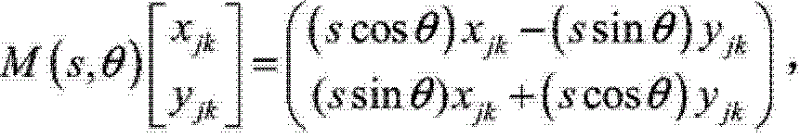
步骤1.2:对齐训练形状向量;通过缩放、旋转和平移的操作使训练形状对齐,使它们尽可能对齐紧密,设xi是训练集中第i个形状中n个点的向量,xi=(xi0,yi0,...xik,yik,...,xin-1,yin-1)T。其中,(xik,yik)是第i个形状中第k个点,给定两个相似形状xi和xj,选择旋转角度θ、缩放s、平移(tx,ty),则M(s,θ)[x]代表旋转角度为θ和缩放比例为s的变换,使以下加权和最小化将xi映射为xj: Step 1.2: Align the training shape vectors; align the training shapes by scaling, rotating and translating operations so that they are aligned as closely as possible, let x i be the vector of n points in the i-th shape in the training set, x i =(x i0 ,y i0 ,...x ik ,y ik ,...,x in-1 ,y in-1 ) T . Among them, (xi ik , y ik ) is the kth point in the i-th shape, given two similar shapes x i and x j , choose the rotation angle θ, scale s, and translate (t x , t y ), then M(s,θ)[x] represents a transformation with rotation θ and scaling s that minimizes the following weighted sum mapping x i to x j :
Ej=(xi-M(s,θ)[xj]-t)TW(xi-M(s,θ)[xj]-t) (1) E j =( xi -M(s,θ)[x j ]-t) T W( xi -M(s,θ)[x j ]-t) (1)
其中,
如果令ax=scosθ,ay=ssinθ,则根据最小二乘法有四个线性等式 If a x =scosθ, a y =ssinθ, then there are four linear equations according to the least square method
其中,
步骤1.3:建立肺部初始轮廓位置的模型;训练形状向量对齐后,利用主成分分析方法找出形状变化的统计信息,据此建立模型; Step 1.3: Establish the model of the initial contour position of the lung; after the training shape vectors are aligned, use the principal component analysis method to find out the statistical information of the shape change, and build the model accordingly;
步骤2:结合灰度信息和形状信息的肺实质分割:同时利用多张特征图像中边界点的灰度与形状信息,使得搜索到的边界灰度、形状信息与训练图像相似; Step 2: Segmentation of lung parenchyma combining grayscale information and shape information: using the grayscale and shape information of boundary points in multiple feature images at the same time, so that the searched boundary grayscale and shape information are similar to the training images;
步骤2.1:提取特征图像;进行主成分分析对数据进行降维,对于图像I中点p附近的点p+△p的灰度可由Taylor展开获得,
由此可得,图像I的二阶Taylor展开为: It can be obtained that the second-order Taylor expansion of image I is:
对图像进行高斯平滑处理,对于图像I(p)进行高斯滤波后的图像为A(p,σ)=(I*G)(p,σ)。滤波图像的n阶偏导数为则根据卷积性质可知: Gaussian smoothing is performed on the image, and the image after Gaussian filtering on the image I(p) is A(p,σ)=(I*G)(p,σ). The nth order partial derivative of the filtered image is According to the convolution properties, we can know:
式中:角标i1,...in表示数据分别对变量求偏导数,把高斯偏导数看作是一个滤波器,高斯偏导数响应的组合构成一个完整的特征描述;对于一个给定尺度参数σ的n-jet特征可以定义为: In the formula: the subscripts i 1 ,...i n indicate that the data calculates the partial derivatives of the variables respectively, and the Gaussian partial derivatives are regarded as a filter, and the combination of the Gaussian partial derivative responses constitutes a complete feature description; for a given The n-jet feature of the scale parameter σ can be defined as:
由此可以看出,当N→∞时,在某一尺度空间中,图像I的局部特征由所有偏导数的组合构成。因此,可以采用高斯偏导数构造一个特征向量来描述局部特征。当偏导数阶数越高时,对图像的描述越准确。但是,如果使用过多的偏导数描述图像,会使得特征向量维数增加。 It can be seen from this that when N → ∞, in a certain scale space, the local features of the image I are composed of the combination of all partial derivatives. Therefore, Gaussian partial derivatives can be used to construct a feature vector to describe local features. When the partial derivative order is higher, the description of the image is more accurate. However, if too many partial derivatives are used to describe the image, the dimension of the feature vector will increase. the
利用局部2-jet特征图像来获取边界点的候选点及各个候选点的灰度代价,局部2-jet特征为: Use the local 2-jet feature image to obtain the candidate points of the boundary points and the gray cost of each candidate point. The local 2-jet features are:
J2[I](p,σ)={I,Ix,Iy,Ixx,Ixy,Iyy} (7) J 2 [I](p,σ)={I,I x ,I y ,I xx ,I xy ,I yy } (7)
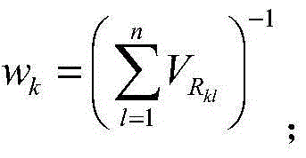
步骤2.2:选取边界点的候选点:对于初始肺边界的每一个点,计算所有特征图像中该点搜索区域内所有像素点的灰度与训练特征图像中相应点灰度的相似程度,选出相似程度最大的点,作为该边界点的候选点。相似程度为所有特征图像中该点周围像素点灰度到训练样本特征图像中相应点周围像素点灰度集合的马氏距离hi: Step 2.2: Select the candidate point of the boundary point: For each point of the initial lung boundary, calculate the similarity between the gray levels of all pixels in the search area of this point in all feature images and the gray level of the corresponding point in the training feature image, and select The point with the greatest similarity is used as the candidate point of the boundary point. The degree of similarity is the Mahalanobis distance h i from the gray level of the pixels around the point in all feature images to the set of gray levels of pixels around the corresponding point in the feature image of the training sample:
步骤2.3:使用动态规划进行肺区域分割;在边界点搜索区域内,像素点的灰度相似性代价为该点周围像素点灰度与训练图像中相应边界点的周围像素点灰度的相似程度hi在边界点搜索区域内,像素点的灰度相似性代价为该点周围像素点灰度与训练图像中相应边界点的周围像素点灰度的相似程度hi;图像中第i个边界点的形状相似性代价定义为: Step 2.3: Use dynamic programming to segment the lung area; in the boundary point search area, the gray similarity cost of the pixel point is the similarity between the gray level of the surrounding pixels of this point and the surrounding pixel gray level of the corresponding boundary point in the training image h i In the boundary point search area, the gray similarity cost of the pixel point is the similarity h i of the gray level of the surrounding pixels of this point and the surrounding pixel gray level of the corresponding boundary point in the training image; the i-th boundary in the image The shape similarity cost of a point is defined as:
式中,vi=pi+1-pi,表示第i个边界点的形状特征,
对于测试图像中第i个边界点pi,在指定的搜索区域内存在m个具有较小灰度相似性代价候选点,则n个边界点就会产生一个n×m的灰度代价矩阵: For the i-th boundary point p i in the test image, there are m candidate points with a smaller gray-scale similarity cost in the specified search area, then n boundary points will generate an n×m gray-scale cost matrix:
式中:
搜索最优轮廓即找一条最佳路径,在矩阵C中每行选一个元素,沿着路径选择的时候,灰度与形状相似性代价的总和最小,即: To search for the optimal contour is to find an optimal path, select one element in each row in the matrix C, and when selecting along the path, the sum of the gray level and shape similarity costs is the smallest, namely:
其中,γ为灰度与形状相似性代价系数。调整γ值,使得这两种代价在边界搜索过程中发挥大致相同的作用; Among them, γ is the gray level and shape similarity cost coefficient. Adjust the value of γ so that these two costs play roughly the same role in the boundary search process;
步骤3:使用B样条多尺度小波变换的特征图像提取;在模型建立过程中,提取有效描述不同尺度骨骼的特征图像是模型建立的基础; Step 3: Feature image extraction using B-spline multi-scale wavelet transform; in the process of model building, extracting feature images that effectively describe bones of different scales is the basis of model building;
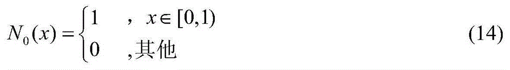
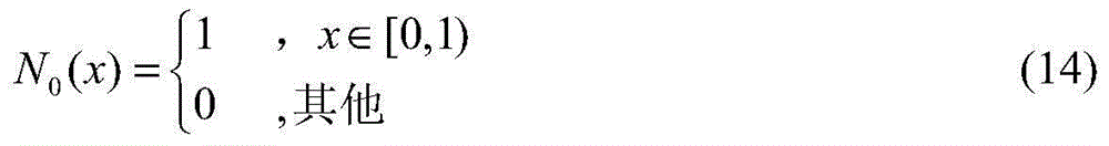
步骤3.1:B样条多尺度小波变换:B样条函数随着样条阶数的增加而快速收敛于高斯函数,其一阶导数可以逼近最优边缘检测算子;利用B样条小波进行多尺度边缘增强;m阶B样条基函数N(m)可定义为: Step 3.1: B-spline multi-scale wavelet transform: The B-spline function quickly converges to a Gaussian function with the increase of the spline order, and its first-order derivative can approach the optimal edge detection operator; use B-spline wavelet for multi-scale Scale edge enhancement; m-order B-spline basis function N(m) can be defined as:
其中,
当m≥1时,m阶B样条函数Nm(x)可用卷积迭代关系表示: When m≥1, the m-order B-spline function N m (x) can be expressed by the convolution iteration relationship:
显然,Nm(x)是非负且紧支撑的,其支撑宽度为suppNm=[0,m+1],支撑中心为(m+1)/2,且Nm关于(m+1)/2中心对称。 Obviously, N m (x) is non-negative and tightly supported, its support width is suppN m =[0,m+1], the support center is (m+1)/2, and N m is about (m+1)/ 2 center symmetrical.
零价B样条的傅里叶变换为则m次B样条的傅里叶形式为: The Fourier transform of the zero-valent B-spline is Then the Fourier form of B-spline of degree m is:
若将m次B样条基Nm(x)平移到Nm[x+(m+1)/2],则对称中心移至坐标原点,傅里叶变换将不再出现上式中的线性相位。但是,当m为偶数时,将出现半整数节点。为避免出现半整数节点,当m为偶数时,将Nm(x)平移到Nm[x+(m+1)/2],则对称中心移至1/2。将Nm(x)整数平移后的函数记为θm(x),其傅里叶变换为: If the m-time B-spline basis N m (x) is translated to N m [x+(m+1)/2], the center of symmetry will move to the coordinate origin, and the Fourier transform will no longer appear in the linear phase in the above formula . However, when m is even, half-integer nodes will appear. To avoid half-integer nodes, when m is an even number, translate N m (x) to N m [x+(m+1)/2], then the center of symmetry will move to 1/2. The function after integer translation of N m (x) is recorded as θ m (x), and its Fourier transform is:
由多分辨率分析得到二尺度关系式
式中,当m为奇数时,ε=0;当m为偶数时,ε=1。由欧拉公式和二项式展开可得低通滤波器为: In the formula, when m is an odd number, ε=0; when m is an even number, ε=1. From Euler's formula and binomial expansion, the low-pass filter can be obtained as:
当m为奇数时,
当m为偶数时,
选取B样条函数的一阶导数作为小波函数,即m+1次B样条函数在2-1尺度上一阶微分函数为m次B样条小波函数: The first-order derivative of the B-spline function is selected as the wavelet function, that is, the first-order differential function of the m+1 B-spline function on the 2-1 scale is the m-order B-spline wavelet function:
其傅里叶变换为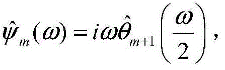

当m是奇数时,

当m=3时,各项滤波器系数为k=-2,-1,0,1,2,gk={0,0,-2,2,0}。由此可见,三阶B样条小波的滤波器的有限长度为5。 When m=3, each filter coefficient is k=-2,-1,0,1,2, g k ={0,0,-2,2,0}. It can be seen that the finite length of the filter of the third-order B-spline wavelet is 5.
求取B样条小波变换滤波器系数: Calculate B-spline wavelet transform filter coefficients:
式中:hk为低通滤波器系数,gk为高通滤波器系数,利用所得hk和gk对图像进行快速小波分解,原始图像的行分别与hk和gk进行卷积,再对其列进行下采样,可以得到两幅子图像,然后沿着列的方向对两幅子图像做滤波并进行下采样,就可以得到四幅1/4大小的输出子图像,对角线细节图像,垂直细节图像,水平细节图像和近似图像; In the formula: h k is the coefficient of the low-pass filter, g k is the coefficient of the high-pass filter, and the obtained h k and g k are used to perform fast wavelet decomposition on the image, and the rows of the original image are convolved with h k and g k respectively, and then By downsampling its column, two sub-images can be obtained, and then the two sub-images are filtered and down-sampled along the direction of the column, and four output sub-images of 1/4 size can be obtained, and the diagonal detail image , the vertical detail image, the horizontal detail image and the approximate image;
步骤3.2:高斯滤波局部2-jet特征图像提取,由于高斯偏导数构造的特征向量能用来描述图像的局部特征,提取不同尺度小波变换后的细节图像的2-jet特征(I,Ix,Iy,Ixx,Ixy,Iyy)图来建立回归模型。根据公式(7)式中,高斯滤波的尺度为σ=2、4; Step 3.2: Gaussian filter local 2-jet feature image extraction, since the feature vector constructed by Gaussian partial derivative can be used to describe the local features of the image, extract the 2-jet features (I, I x , I y , I xx , I xy , I yy ) graph to build a regression model. According to the formula (7), the scale of the Gaussian filter is σ=2, 4;
步骤权:使用支持向量回归进行骨骼图像的预测,通过求得回归函数f(x)=ω·x+b,建立骨骼模型:设样本集为(xi,yi),i=1,2,...,l,xi∈Rn,样本集S是ε-不敏感损失函数的线性近似。当线性回归函数f(x)=ω·x+b拟合(xi,yi)时,假设所有训练数据的拟合误差精度为ε,即: Step right: use support vector regression to predict the bone image, and establish the bone model by obtaining the regression function f(x)=ω·x+b: set the sample set as ( xi , y i ), i=1,2 ,...,l, xi ∈ R n , the sample set S is a linear approximation of the ε-insensitive loss function. When the linear regression function f(x)=ω·x+b fits ( xi , y i ), it is assumed that the fitting error accuracy of all training data is ε, namely:
|yi-f(xi)|≤εi=1,2,...,l (22) |y i -f(x i )|≤εi=1,2,...,l (22)
让di表示点(xi,yi)∈S到超平面f(x)的距离: Let d i denote the distance of a point ( xi , y i ) ∈ S to the hyperplane f(x):
因为S集是ε-线性近似,所以有|<w,x>+b-f(xi)|≤ε,i=1,...,m。可以得到: Since the S set is an ε-linear approximation, there are |<w,x>+b-f(xi)|≤ε,i=1,...,m. Can get:
于是有 So there are
(23)式表明
最优超平面是通过最大化

求下面的最优化问题: Find the following optimization problem:
约束为|<w,x>+b-yi|≤ε,i=1,...,m。另外,考虑拟合误差的情况,引入松弛因子

因而,标准ε不敏感支持向量回归机可以表示为: Therefore, the standard ε-insensitive support vector regression machine can be expressed as:
其中,C>0为平衡因子。引入拉格朗日函数为: Among them, C>0 is the balance factor. Introduce the Lagrangian function as:
其中,αi,
C-αi-γi=0,i=1,...,l (31) C-α i -γ i =0,i=1,...,l (31)
将(29)-(32)代入到(28)中,得到优化问题的对偶形式为: Substituting (29)-(32) into (28), the dual form of the optimization problem is obtained as:
约束为: Constraints are:
由于骨骼灰度预测为非线性回归,所以先使用一个非线性映射φ,把数据映射到一个高维特征空间,然后在高维特征空间进行线性回归建立模型。由于在上面的优化过程中,只考虑到高维特征空间中的内积运算,因此用一个核函数k(x,y)代替<φ(x),φ(y)>就可以实现非线性回归。于是,非线性回归的优化方程为最大化下面的函数: Since the bone grayscale prediction is a nonlinear regression, a nonlinear mapping φ is first used to map the data to a high-dimensional feature space, and then a linear regression is performed in the high-dimensional feature space to build a model. Since only the inner product operation in the high-dimensional feature space is considered in the above optimization process, nonlinear regression can be realized by replacing <φ(x),φ(y)> with a kernel function k(x,y) . Therefore, the optimization equation for nonlinear regression is to maximize the following function:
其约束条件为(32)。求解出α的值后,就可以得到f(x): Its constraints are (32). After solving the value of α, f(x) can be obtained:
通常情况下,大部分αi或
于是得到b的计算式如下: So the calculation formula of b is as follows:
用任意一个支持向量可以计算出b的值,得到回归函数f(x);建立预测模型后,可以根据肺部x光图像的灰度值分布来预测产生骨结构图像; The value of b can be calculated with any support vector, and the regression function f(x) can be obtained; after the prediction model is established, the bone structure image can be predicted according to the gray value distribution of the lung X-ray image;
步骤5:对正常胸片与预测的骨骼图像做图像减法来预测的软组织图像。 Step 5: Perform image subtraction on the normal chest radiograph and the predicted bone image to obtain the predicted soft tissue image. the
所述步骤1.2:对齐训练形状向量的具体步骤如下: The step 1.2: The specific steps of aligning the training shape vectors are as follows:
所述的将分块的数据映射到特征空间的具体方法如下: The specific method of mapping the block data to the feature space is as follows:
步骤1.2.1:旋转、缩放和平移每个肺区域形状,使其与训练集中的第一个形状对齐; Step 1.2.1: Rotate, scale and translate each lung region shape to align with the first shape in the training set;
步骤1.2.2:根据对齐形状,计算平均形状; Step 1.2.2: Calculate the average shape according to the aligned shape;
步骤1.2.3:旋转、缩放和平移平均形状使其与第一个形状对齐; Step 1.2.3: Rotate, scale and translate the average shape to align with the first shape;
步骤1.2.权:重新将每个形状与当前平均形状对齐; Step 1.2. Weight: Re-align each shape with the current average shape;
步骤1.2.5:如果过程收敛或者到指定循环次数,退出;否则转到步骤。 Step 1.2.5: If the process converges or reaches the specified number of cycles, exit; otherwise go to step. the
所述步骤3中对胸部x光图像做三尺度小波分解。 In the step 3, a three-scale wavelet decomposition is performed on the chest x-ray image. the
本发明的优点为:本发明先对双能剪影图像中的正常胸片建立肺部轮廓模型,再应用三阶B样条小波变换对图像做三尺度小波分解,将分解后的图像使用2-jet方法提取特征图像, 再使用支持向量回归机建立骨骼模型,将骨骼模型应用到X光图像中,从而提取对应的预测骨骼图像,最后用X光图像与预测的骨骼图像做图像减法从而得到预测的软组织图像。因为抑制骨骼方法大都采用神经网络方法,而此方法易陷入局部最优,训练结果不太稳定,所以本专利采用支持向量回归机来进行骨骼预测,得到了更优的结果。 The advantages of the present invention are: the present invention first establishes the lung contour model on the normal chest radiograph in the dual-energy silhouette image, and then applies the third-order B-spline wavelet transform to perform three-scale wavelet decomposition on the image, and uses 2- The jet method extracts the feature image, and then uses the support vector regression machine to establish the bone model, applies the bone model to the X-ray image, thereby extracting the corresponding predicted bone image, and finally uses the X-ray image and the predicted bone image to perform image subtraction to obtain the prediction soft tissue images. Because most of the bone suppression methods use the neural network method, and this method is easy to fall into a local optimum, and the training results are not stable, so this patent uses a support vector regression machine for bone prediction, and better results are obtained. the
附图说明 Description of drawings
图1是本发明的总体流程图; Fig. 1 is overall flow chart of the present invention;
图2是本发明的肺区分割流程图; Fig. 2 is the segmentation flow chart of lung area of the present invention;
图3是本发明中高斯滤波局部2-jet提取特征图像示意图; Fig. 3 is a schematic diagram of feature image extracted by Gaussian filtering local 2-jet in the present invention;
图4是本发明中最优近似超平面的示意图; Fig. 4 is the schematic diagram of optimal approximation hyperplane among the present invention;
图5是本发明中支持向量回归示意图。 Fig. 5 is a schematic diagram of support vector regression in the present invention. the
具体实施方式Detailed ways
如图1至图5所示,本发明采取按如下步骤进行: As shown in Figures 1 to 5, the present invention takes the following steps to carry out:
步骤1:模型肺部初始轮廓位置的确定; Step 1: Determination of the initial contour position of the model lung;
步骤1.1:标记训练集中每张图像肺边界的边界点; Step 1.1: Mark the boundary points of the lung boundaries of each image in the training set;
步骤1.2:对齐训练形状向量;通过缩放、旋转和平移的操作使训练形状对齐,使它们尽可能对齐紧密,设xi是训练集中第i个形状中n个点的向量,xi=(xi0,yi0,...xik,yik,...,xin-1,yin-1)T。其中,(xik,yik)是第i个形状中第k个点,给定两个相似形状xi和xj,选择旋转角度θ、缩放s、平移(tx,ty),则M(s,θ)[x]代表旋转角度为θ和缩放比例为s的变换,使以下加权和最小化将xi映射为xj: Step 1.2: Align the training shape vectors; align the training shapes by scaling, rotating and translating operations so that they are aligned as closely as possible, let x i be the vector of n points in the i-th shape in the training set, x i =(x i0 ,y i0 ,...x ik ,y ik ,...,x in-1 ,y in-1 ) T . Among them, (xi ik , y ik ) is the kth point in the i-th shape, given two similar shapes x i and x j , choose the rotation angle θ, scale s, and translate (t x , t y ), then M(s,θ)[x] represents a transformation with rotation θ and scaling s that minimizes the following weighted sum mapping x i to x j :
Ej=(xi-M(s,θ)[xj]-t)TW(xi-M(s,θ)[xj]-t) (1) E j =( xi -M(s,θ)[x j ]-t) T W( xi -M(s,θ)[x j ]-t) (1)
其中,
如果令ax=scosθ,ay=ssinθ,则根据最小二乘法有四个线性等式 If a x =scosθ, a y =ssinθ, then there are four linear equations according to the least square method
其中,
步骤1.3:建立肺部初始轮廓位置的模型;训练形状向量对齐后,利用主成分分析方法找出形状变化的统计信息,据此建立模型; Step 1.3: Establish the model of the initial contour position of the lung; after the training shape vectors are aligned, use the principal component analysis method to find out the statistical information of the shape change, and build the model accordingly;
步骤2:结合灰度信息和形状信息的肺实质分割:同时利用多张特征图像中边界点的灰度与形状信息,使得搜索到的边界灰度、形状信息与训练图像相似; Step 2: Lung parenchyma segmentation combining grayscale information and shape information: using the grayscale and shape information of boundary points in multiple feature images at the same time, so that the searched boundary grayscale and shape information are similar to the training images;
步骤2.1:提取特征图像;进行主成分分析对数据进行降维,对于图像I中点p附近的点p+△p的灰度可由Taylor展开获得,
(2) (2)
由此可得,图像I的二阶Taylor展开为: It can be obtained that the second-order Taylor expansion of image I is:
对图像进行高斯平滑处理,对于图像I(p)进行高斯滤波后的图像为A(p,σ)=(I*G)(p,σ)。滤波图像的n阶偏导数为
式中:角标i1,...in表示数据分别对变量求偏导数,把高斯偏导数看作是一个滤波器,高斯偏导数响应的组合构成一个完整的特征描述;对于一个给定尺度参数σ的n-jet特征可以定义为: In the formula: the subscripts i 1 ,...i n indicate that the data calculates the partial derivatives of the variables respectively, and the Gaussian partial derivatives are regarded as a filter, and the combination of the Gaussian partial derivative responses constitutes a complete feature description; for a given The n-jet feature of the scale parameter σ can be defined as:
由此可以看出,当N→∞时,在某一尺度空间中,图像I的局部特征由所有偏导数的组合构成。因此,可以采用高斯偏导数构造一个特征向量来描述局部特征。当偏导数阶数越高时,对图像的描述越准确。但是,如果使用过多的偏导数描述图像,会使得特征向量维数增加。 It can be seen from this that when N → ∞, in a certain scale space, the local features of the image I are composed of the combination of all partial derivatives. Therefore, Gaussian partial derivatives can be used to construct a feature vector to describe local features. When the partial derivative order is higher, the description of the image is more accurate. However, if too many partial derivatives are used to describe the image, the dimension of the feature vector will increase. the
利用局部2-jet特征图像来获取边界点的候选点及各个候选点的灰度代价,局部2-jet特征为: Use the local 2-jet feature image to obtain the candidate points of the boundary points and the gray cost of each candidate point. The local 2-jet features are:
J2[I](p,σ)={I,Ix,Iy,Ixx,Ixy,Iyy} (7) J 2 [I](p,σ)={I,I x ,I y ,I xx ,I xy ,I yy } (7)
步骤2.2:选取边界点的候选点:对于初始肺边界的每一个点,计算所有特征图像中该点搜索区域内所有像素点的灰度与训练特征图像中相应点灰度的相似程度,选出相似程度最大的点,作为该边界点的候选点。相似程度为所有特征图像中该点周围像素点灰度到训练样本特征图像中相应点周围像素点灰度集合的马氏距离hi: Step 2.2: Select the candidate point of the boundary point: For each point of the initial lung boundary, calculate the similarity between the gray levels of all pixels in the search area of this point in all feature images and the gray level of the corresponding point in the training feature image, and select The point with the greatest similarity is used as the candidate point of the boundary point. The degree of similarity is the Mahalanobis distance h i from the gray level of the pixels around the point in all feature images to the set of gray levels of pixels around the corresponding point in the feature image of the training sample:
步骤2.3:使用动态规划进行肺区域分割;在边界点搜索区域内,像素点的灰度相似性代价为该点周围像素点灰度与训练图像中相应边界点的周围像素点灰度的相似程度hi在边界点搜索区域内,像素点的灰度相似性代价为该点周围像素点灰度与训练图像中相应边界点的周围像素点灰度的相似程度hi;图像中第i个边界点的形状相似性代价定义为: Step 2.3: Use dynamic programming to segment the lung area; in the boundary point search area, the gray similarity cost of the pixel point is the similarity between the gray level of the surrounding pixels of this point and the surrounding pixel gray level of the corresponding boundary point in the training image h i In the boundary point search area, the gray similarity cost of the pixel point is the similarity h i of the gray level of the surrounding pixels of this point and the surrounding pixel gray level of the corresponding boundary point in the training image; the i-th boundary in the image The shape similarity cost of a point is defined as:
式中,vi=pi+1-pi,表示第i个边界点的形状特征,
对于测试图像中第i个边界点pi,在指定的搜索区域内存在m个具有较小灰度相似性代价候选点,则n个边界点就会产生一个n×m的灰度代价矩阵: For the i-th boundary point p i in the test image, there are m candidate points with a smaller gray-scale similarity cost in the specified search area, then n boundary points will generate an n×m gray-scale cost matrix:
式中:为在特征图像上,以点pi为圆心,rc为半径的圆上的nc个点的灰度,k=1......nc。 
搜索最优轮廓即找一条最佳路径,在矩阵C中每行选一个元素,沿着路径选择的时候,灰度与形状相似性代价的总和最小,即: To search for the optimal contour is to find an optimal path, select one element in each row in the matrix C, and when selecting along the path, the sum of the gray level and shape similarity costs is the smallest, namely:
其中,γ为灰度与形状相似性代价系数。调整γ值,使得这两种代价在边界搜索过程中发挥大致相同的作用; Among them, γ is the gray level and shape similarity cost coefficient. Adjust the value of γ so that these two costs play roughly the same role in the boundary search process;
步骤3:使用B样条多尺度小波变换的特征图像提取;在模型建立过程中,提取有效描述不同尺度骨骼的特征图像是模型建立的基础; Step 3: Feature image extraction using B-spline multi-scale wavelet transform; in the process of model building, extracting feature images that effectively describe bones of different scales is the basis of model building;
步骤3.1:B样条多尺度小波变换:B样条函数随着样条阶数的增加而快速收敛于高斯函数,其一阶导数可以逼近最优边缘检测算子;利用B样条小波进行多尺度边缘增强;m阶B样条基函数N(m)可定义为: Step 3.1: B-spline multi-scale wavelet transform: The B-spline function quickly converges to a Gaussian function with the increase of the spline order, and its first-order derivative can approach the optimal edge detection operator; use B-spline wavelet for multi-scale Scale edge enhancement; m-order B-spline basis function N(m) can be defined as:
其中,
当m≥1时,m阶B样条函数Nm(x)可用卷积迭代关系表示: When m≥1, the m-order B-spline function N m (x) can be expressed by the convolution iteration relationship:

显然,Nm(x)是非负且紧支撑的,其支撑宽度为suppNm=[0,m+1],支撑中心为(m+1)/2,且Nm关于(m+1)/2中心对称。 Obviously, N m (x) is non-negative and tightly supported, its support width is suppN m =[0,m+1], the support center is (m+1)/2, and N m is about (m+1)/ 2 center symmetrical.
零阶B样条的傅里叶变换为则m次B样条的傅里叶形式为: The Fourier transform of the zero-order B-spline is Then the Fourier form of B-spline of degree m is:
若将m次B样条基Nm(x)平移到Nm[x+(m+1)/2],则对称中心移至坐标原点,傅里叶变换将不再出现上式中的线性相位。但是,当m为偶数时,将出现半整数节点。为避免出现半整数节点,当m为偶数时,将Nm(x)平移到Nm[x+(m+1)/2],则对称中心移至1/2。将Nm(x)整数 平移后的函数记为θm(x),其傅里叶变换为: If the m-time B-spline basis N m (x) is translated to N m [x+(m+1)/2], the center of symmetry will move to the coordinate origin, and the Fourier transform will no longer appear in the linear phase in the above formula . However, when m is even, half-integer nodes will appear. To avoid half-integer nodes, when m is an even number, translate N m (x) to N m [x+(m+1)/2], then the center of symmetry will move to 1/2. The function after integer translation of N m (x) is recorded as θ m (x), and its Fourier transform is:
由多分辨率分析得到二尺度关系式可求得: The two-scale relationship obtained by multiresolution analysis can be obtained:
式中,当m为奇数时,ε=0;当m为偶数时,ε=1。由欧拉公式和二项式展开可得低通滤波器为: In the formula, when m is an odd number, ε=0; when m is an even number, ε=1. From Euler's formula and binomial expansion, the low-pass filter can be obtained as:
当m为奇数时,
当m为偶数时, When m is an even number,
选取B样条函数的一阶导数作为小波函数,即m+1次B样条函数在2-1尺度上一阶微分函数为m次B样条小波函数: The first-order derivative of the B-spline function is selected as the wavelet function, that is, the first-order differential function of the m+1 B-spline function on the 2-1 scale is the m-order B-spline wavelet function:
其傅里叶变换为

当m是奇数时,
当m=3时,各项滤波器系数为k=-2,-1,0,1,2,
求取3阶B样条小波变换滤波器系数: Calculate the third-order B-spline wavelet transform filter coefficients:
式中:hk为低通滤波器系数,gk为高通滤波器系数,利用所得hk和gk对图像进行快速小波分解,原始图像的行分别与hk和gk进行卷积,再对其列进行下采样,可以得到两幅子图像,然后沿着列的方向对两幅子图像做滤波并进行下采样,就可以得到四幅1/4大小的输出子图像,对角线细节图像,垂直细节图像,水平细节图像和近似图像; In the formula: h k is the coefficient of the low-pass filter, g k is the coefficient of the high-pass filter, and the obtained h k and g k are used to perform fast wavelet decomposition on the image, and the rows of the original image are convolved with h k and g k respectively, and then By downsampling its column, two sub-images can be obtained, and then the two sub-images are filtered and down-sampled along the direction of the column, and four output sub-images of 1/4 size can be obtained, and the diagonal detail image , the vertical detail image, the horizontal detail image and the approximate image;
本实施例对胸部x光图像做三尺度小波分解,获得12张小波分解图像,其中3张近似图像,3张水平细节图像,3张垂直细节图像,3张对角线细节图像。由于在胸部x光图像中,很少有呈现对角线分布的骨骼结构。因此,不提取对角线细节图像的特征。 In this embodiment, three-scale wavelet decomposition is performed on chest X-ray images to obtain 12 wavelet-decomposed images, including 3 approximate images, 3 horizontal detail images, 3 vertical detail images, and 3 diagonal detail images. Because in the chest x-ray image, there are few skeletal structures that show a diagonal distribution. Therefore, features of diagonal detail images are not extracted. the
步骤3.2:高斯滤波局部2-jet特征图像提取,由于高斯偏导数构造的特征向量能用来描述图像的局部特征,提取不同尺度小波变换后的细节图像的2-jet特征(I,Ix,Iy,Ixx,Ixy,Iyy)图来建立回归模型。根据公式(7)式中,高斯滤波的尺度为σ=2、4; Step 3.2: Gaussian filter local 2-jet feature image extraction, since the feature vector constructed by Gaussian partial derivative can be used to describe the local features of the image, extract the 2-jet features (I, I x , I y , I xx , I xy , I yy ) graph to build a regression model. According to the formula (7), the scale of the Gaussian filter is σ=2, 4;
步骤权:使用支持向量回归进行骨骼图像的预测,通过求得回归函数f(x)=ω·x+b,建立骨骼模型;设样本集为(xi,yi),i=1,2,...,l,xi∈Rn,样本集S是ε-不敏感损失函数的线性近似。当线性回归函数f(x)=ω·x+b拟合(xi,yi)时,假设所有训练数据的拟合误差精度为ε,即: Step right: use support vector regression to predict the bone image, and establish the bone model by obtaining the regression function f(x)=ω·x+b; set the sample set as ( xi , y i ), i=1,2 ,...,l, xi ∈ R n , the sample set S is a linear approximation of the ε-insensitive loss function. When the linear regression function f(x)=ω·x+b fits ( xi , y i ), it is assumed that the fitting error accuracy of all training data is ε, namely:
|yi-f(xi)|≤εi=1,2,...,l (22) |y i -f(x i )|≤εi=1,2,...,l (22)
让di表示点(xi,yi)∈S到超平面f(x)的距离: Let d i denote the distance of a point ( xi , y i ) ∈ S to the hyperplane f(x):
因为S集是ε-线性近似,所以有|<w,x>+b-f(xi)|≤ε,i=1,...,m。可以得到: Since the set S is an ε-linear approximation, there is |<w,x>+bf(x i )|≤ε,i=1,...,m. can get:
于是有 So there are
(23)式表明
最优超平面是通过最大化

求下面的最优化问题: Find the following optimization problem:
约束为|<w,x>+b-yi|≤ε,i=1,...,m。另外,考虑拟合误差的情况,引入松弛因子当划分有误差时,
因而,标准ε不敏感支持向量回归机可以表示为: Therefore, the standard ε-insensitive support vector regression machine can be expressed as:
其中,C>0为平衡因子。引入拉格朗日函数为: Among them, C>0 is the balance factor. Introduce the Lagrangian function as:
其中,αi,
C-αi-γi=0,i=1,...,l (31) C-α i -γ i =0,i=1,...,l (31)
将(29)-(32)代入到(28)中,得到优化问题的对偶形式为: Substituting (29)-(32) into (28), the dual form of the optimization problem is obtained as:
约束为: Constraints are:
由于骨骼灰度预测为非线性回归,所以先使用一个非线性映射φ,把数据映射到一个高维特征空间,然后在高维特征空间进行线性回归建立模型。由于在上面的优化过程中,只考虑到高维特征空间中的内积运算,因此用一个核函数k(x,y)代替<φ(x),φ(y)>就可以实现非线性回归。于是,非线性回归的优化方程为最大化下面的函数: Since the bone grayscale prediction is a nonlinear regression, a nonlinear mapping φ is first used to map the data to a high-dimensional feature space, and then a linear regression is performed in the high-dimensional feature space to build a model. Since only the inner product operation in the high-dimensional feature space is considered in the above optimization process, nonlinear regression can be realized by replacing <φ(x),φ(y)> with a kernel function k(x,y) . Therefore, the optimization equation for nonlinear regression is to maximize the following function:
其约束条件为(32)。求解出α的值后,就可以得到f(x): Its constraints are (32). After solving the value of α, f(x) can be obtained:
通常情况下,大部分αi或
于是得到b的计算式如下: So the calculation formula of b is as follows:
用任意一个支持向量可以计算出b的值,得到回归函数f(x);建立预测模型后,可以根据肺部x光图像的灰度值分布来预测产生骨结构图像; The value of b can be calculated with any support vector, and the regression function f(x) can be obtained; after the prediction model is established, the bone structure image can be predicted according to the gray value distribution of the lung X-ray image;
步骤5:对正常胸片与预测的骨骼图像做图像减法来预测的软组织图像。 Step 5: Perform image subtraction on the normal chest radiograph and the predicted bone image to obtain the predicted soft tissue image. the
所述步骤1.2:对齐训练形状向量的具体步骤如下: The step 1.2: The specific steps of aligning the training shape vectors are as follows:
所述的将分块的数据映射到特征空间的具体方法如下: The specific method of mapping the block data to the feature space is as follows:
步骤1.2.1:旋转、缩放和平移每个肺区域形状,使其与训练集中的第一个形状对齐; Step 1.2.1: Rotate, scale and translate each lung region shape to align with the first shape in the training set;
步骤1.2.2:根据对齐形状,计算平均形状; Step 1.2.2: Calculate the average shape according to the aligned shape;
步骤1.2.3:旋转、缩放和平移平均形状使其与第一个形状对齐; Step 1.2.3: Rotate, scale and translate the average shape to align with the first shape;
步骤1.2.权:重新将每个形状与当前平均形状对齐; Step 1.2. Weight: Re-align each shape with the current average shape;
步骤1.2.5:如果过程收敛或者到指定循环次数,退出;否则转到步骤。 Step 1.2.5: If the process converges or reaches the specified number of cycles, exit; otherwise go to step. the
所述步骤3中对胸部x光图像做三尺度小波分解。 In the step 3, a three-scale wavelet decomposition is performed on the chest x-ray image. the
Claims (5)


Priority Applications (1)
| Application Number | Priority Date | Filing Date | Title |
|---|---|---|---|
| CN201410007747.XA CN103824281B (en) | 2014-01-07 | A kind of method of skeleton suppression in chest x-ray image |
Applications Claiming Priority (1)
| Application Number | Priority Date | Filing Date | Title |
|---|---|---|---|
| CN201410007747.XA CN103824281B (en) | 2014-01-07 | A kind of method of skeleton suppression in chest x-ray image |
Publications (2)
| Publication Number | Publication Date |
|---|---|
| CN103824281A true CN103824281A (en) | 2014-05-28 |
| CN103824281B CN103824281B (en) | 2016-11-30 |
Family
ID=
Cited By (14)
| Publication number | Priority date | Publication date | Assignee | Title |
|---|---|---|---|---|
| CN104166994A (en) * | 2014-07-29 | 2014-11-26 | 沈阳航空航天大学 | Bone inhibition method based on training sample optimization |
| CN106023200A (en) * | 2016-05-19 | 2016-10-12 | 四川大学 | Poisson model-based X-ray chest image rib inhibition method |
| CN106340015A (en) * | 2016-08-30 | 2017-01-18 | 沈阳东软医疗系统有限公司 | Key point positioning method and device |
| CN107038692A (en) * | 2017-04-16 | 2017-08-11 | 南方医科大学 | X-ray rabat bone based on wavelet decomposition and convolutional neural networks suppresses processing method |
| CN109191389A (en) * | 2018-07-31 | 2019-01-11 | 浙江杭钢健康产业投资管理有限公司 | A kind of x-ray image adaptive local Enhancement Method |
| CN109242867A (en) * | 2018-08-09 | 2019-01-18 | 杭州电子科技大学 | A kind of hand bone automatic division method based on template |
| CN109358605A (en) * | 2018-11-09 | 2019-02-19 | 电子科技大学 | Control system calibration method based on sixth-order B-spline wavelet neural network |
| CN109919961A (en) * | 2019-02-22 | 2019-06-21 | 北京深睿博联科技有限责任公司 | A kind of processing method and processing device for aneurysm region in encephalic CTA image |
| CN111080569A (en) * | 2019-12-24 | 2020-04-28 | 北京推想科技有限公司 | Bone-suppression image generation method and device, storage medium and electronic equipment |
| CN112529818A (en) * | 2020-12-25 | 2021-03-19 | 万里云医疗信息科技(北京)有限公司 | Bone shadow inhibition method, device, equipment and storage medium based on neural network |
| CN115115841A (en) * | 2022-08-30 | 2022-09-27 | 苏州朗开医疗技术有限公司 | Shadow spot image processing and analyzing method and system |
| KR20220165117A (en) * | 2021-06-07 | 2022-12-14 | 연세대학교 산학협력단 | Method and apparatus for decomposing multi-material based on dual-energy technique |
| US12082958B2 (en) | 2022-01-03 | 2024-09-10 | Electronics And Telecommunications Research Institute | System and method for detecting internal load by using X-ray image of container |
| CN118969279A (en) * | 2024-08-16 | 2024-11-15 | 静宁县中医医院 | A method for evaluating bone status recovery after bone injury healing |
Citations (4)
| Publication number | Priority date | Publication date | Assignee | Title |
|---|---|---|---|---|
| US7155042B1 (en) * | 1999-04-21 | 2006-12-26 | Auckland Uniservices Limited | Method and system of measuring characteristics of an organ |
| US20070058850A1 (en) * | 2002-12-10 | 2007-03-15 | Hui Luo | Method for automatic construction of 2d statistical shape model for the lung regions |
| JP2009273644A (en) * | 2008-05-14 | 2009-11-26 | Toshiba Corp | Medical imaging apparatus, medical image processing device, and medical image processing program |
| CN103366348A (en) * | 2013-07-19 | 2013-10-23 | 南方医科大学 | Processing method and processing device for restraining bone image in X-ray image |
Patent Citations (4)
| Publication number | Priority date | Publication date | Assignee | Title |
|---|---|---|---|---|
| US7155042B1 (en) * | 1999-04-21 | 2006-12-26 | Auckland Uniservices Limited | Method and system of measuring characteristics of an organ |
| US20070058850A1 (en) * | 2002-12-10 | 2007-03-15 | Hui Luo | Method for automatic construction of 2d statistical shape model for the lung regions |
| JP2009273644A (en) * | 2008-05-14 | 2009-11-26 | Toshiba Corp | Medical imaging apparatus, medical image processing device, and medical image processing program |
| CN103366348A (en) * | 2013-07-19 | 2013-10-23 | 南方医科大学 | Processing method and processing device for restraining bone image in X-ray image |
Non-Patent Citations (6)
| Title |
|---|
| CHEN SHENG ET AL.: "Bone suppression in chest radiographs by means of anatomically specific multiple massive-training ANNs", 《2012 21ST INTERNATIONAL CONFERENCE ON PATTERN RECOGNITION(ICPR 2012)》 * |
| JIANN-SHU LEE ET AL.: "a nonparametric-based rib suppression method for chest radiographs", 《COMPUTERS & MATHEMATICS WITH APPLICATIONS》 * |
| M. LOOG ET AL.: "Filter learning:application to suppression of bony structures from chest radiographs", 《MEDICAL IMAGE ANALYSIS》 * |
| TAHIR RASHEED ET AL.: "Rib suppression in frontal chest radiographs:a blind source separation approach", 《2007 9TH INTERNATIONAL SYMPOSIUM ON SIGNAL PROCESSING ADN ITS APPLICATIONS(ISSPA)》 * |
| 李锋 等: "人手部骨组织建模的B样条拟合方法研究", 《计算机仿真》 * |
| 杨金宝: "基于灰度相似性测度的医学图像配准技术研究", 《中国博士学位论文全文数据库 信息科技辑》 * |
Cited By (19)
| Publication number | Priority date | Publication date | Assignee | Title |
|---|---|---|---|---|
| CN104166994B (en) * | 2014-07-29 | 2017-04-05 | 沈阳航空航天大学 | A kind of bone suppressing method optimized based on training sample |
| CN104166994A (en) * | 2014-07-29 | 2014-11-26 | 沈阳航空航天大学 | Bone inhibition method based on training sample optimization |
| CN106023200A (en) * | 2016-05-19 | 2016-10-12 | 四川大学 | Poisson model-based X-ray chest image rib inhibition method |
| CN106023200B (en) * | 2016-05-19 | 2019-06-28 | 四川大学 | A kind of x-ray chest radiograph image rib cage suppressing method based on Poisson model |
| CN106340015B (en) * | 2016-08-30 | 2019-02-19 | 沈阳东软医疗系统有限公司 | A kind of localization method and device of key point |
| CN106340015A (en) * | 2016-08-30 | 2017-01-18 | 沈阳东软医疗系统有限公司 | Key point positioning method and device |
| CN107038692A (en) * | 2017-04-16 | 2017-08-11 | 南方医科大学 | X-ray rabat bone based on wavelet decomposition and convolutional neural networks suppresses processing method |
| CN109191389A (en) * | 2018-07-31 | 2019-01-11 | 浙江杭钢健康产业投资管理有限公司 | A kind of x-ray image adaptive local Enhancement Method |
| CN109242867A (en) * | 2018-08-09 | 2019-01-18 | 杭州电子科技大学 | A kind of hand bone automatic division method based on template |
| CN109358605A (en) * | 2018-11-09 | 2019-02-19 | 电子科技大学 | Control system calibration method based on sixth-order B-spline wavelet neural network |
| CN109919961A (en) * | 2019-02-22 | 2019-06-21 | 北京深睿博联科技有限责任公司 | A kind of processing method and processing device for aneurysm region in encephalic CTA image |
| CN111080569A (en) * | 2019-12-24 | 2020-04-28 | 北京推想科技有限公司 | Bone-suppression image generation method and device, storage medium and electronic equipment |
| CN111080569B (en) * | 2019-12-24 | 2021-03-19 | 推想医疗科技股份有限公司 | Bone-suppression image generation method and device, storage medium and electronic equipment |
| CN112529818A (en) * | 2020-12-25 | 2021-03-19 | 万里云医疗信息科技(北京)有限公司 | Bone shadow inhibition method, device, equipment and storage medium based on neural network |
| KR20220165117A (en) * | 2021-06-07 | 2022-12-14 | 연세대학교 산학협력단 | Method and apparatus for decomposing multi-material based on dual-energy technique |
| KR102590461B1 (en) | 2021-06-07 | 2023-10-16 | 연세대학교 산학협력단 | Method and apparatus for decomposing multi-material based on dual-energy technique |
| US12082958B2 (en) | 2022-01-03 | 2024-09-10 | Electronics And Telecommunications Research Institute | System and method for detecting internal load by using X-ray image of container |
| CN115115841A (en) * | 2022-08-30 | 2022-09-27 | 苏州朗开医疗技术有限公司 | Shadow spot image processing and analyzing method and system |
| CN118969279A (en) * | 2024-08-16 | 2024-11-15 | 静宁县中医医院 | A method for evaluating bone status recovery after bone injury healing |
Similar Documents
| Publication | Publication Date | Title |
|---|---|---|
| US11284849B2 (en) | Dual energy x-ray coronary calcium grading | |
| CN107038692A (en) | X-ray rabat bone based on wavelet decomposition and convolutional neural networks suppresses processing method | |
| US20170337686A1 (en) | Kind of x-ray chest image rib suppression method based on poisson model | |
| Fan et al. | COVID-19 detection from X-ray images using multi-kernel-size spatial-channel attention network | |
| WO2017084222A1 (en) | Convolutional neural network-based method for processing x-ray chest radiograph bone suppression | |
| US20120027278A1 (en) | Methods, systems, and computer readable media for mapping regions in a model of an object comprising an anatomical structure from one image data set to images used in a diagnostic or therapeutic intervention | |
| CN107403201A (en) | Tumour radiotherapy target area and jeopardize that organ is intelligent, automation delineation method | |
| CN109559292A (en) | Multi-modality images fusion method based on convolution rarefaction representation | |
| CN103034989B (en) | Low-dose CBCT image denoising method based on high-quality prior image | |
| CN106373163B (en) | A low-dose CT imaging method based on the distinctive feature representation of 3D projection images | |
| WO2015106374A1 (en) | Multidimensional texture extraction method based on brain nuclear magnetic resonance images | |
| CN102842122A (en) | Real image enhancing method based on wavelet neural network | |
| Zhou et al. | Generation of virtual dual energy images from standard single-shot radiographs using multi-scale and conditional adversarial network | |
| Wu et al. | Fracture detection in traumatic pelvic CT images | |
| El-Baz et al. | A novel approach for automatic follow-up of detected lung nodules | |
| Saha et al. | A survey on artificial intelligence in pulmonary imaging | |
| Sammouda | Segmentation and analysis of CT chest images for early lung cancer detection | |
| CN104166994B (en) | A kind of bone suppressing method optimized based on training sample | |
| Nageswara Reddy et al. | BRAIN MR IMAGE SEGMENTATION BY MODIFIED ACTIVE CONTOURS AND CONTOURLET TRANSFORM. | |
| JP2008511395A (en) | Method and system for motion correction in a sequence of images | |
| CN103514607A (en) | Dynamic contrast enhancement magnetic resonance image detection method | |
| Balakrishnan et al. | Liver segmentation using Mnet for cirrhosis | |
| CN103824281B (en) | A kind of method of skeleton suppression in chest x-ray image | |
| CN103824281A (en) | Bone inhibition method in chest X-ray image | |
| Zhou et al. | Towards cross-scale attention and surface supervision for fractured bone segmentation in CT |
Legal Events
| Date | Code | Title | Description |
|---|---|---|---|
| C06 | Publication | ||
| PB01 | Publication | ||
| C10 | Entry into substantive examination | ||
| SE01 | Entry into force of request for substantive examination | ||
| C14 | Grant of patent or utility model | ||
| GR01 | Patent grant | ||
| CF01 | Termination of patent right due to non-payment of annual fee |
Granted publication date: 20161130 Termination date: 20220107 |
|
| CF01 | Termination of patent right due to non-payment of annual fee |