CN103528587A - Autonomous integrated navigation system - Google Patents
Autonomous integrated navigation system Download PDFInfo
- Publication number
- CN103528587A CN103528587A CN201310502827.8A CN201310502827A CN103528587A CN 103528587 A CN103528587 A CN 103528587A CN 201310502827 A CN201310502827 A CN 201310502827A CN 103528587 A CN103528587 A CN 103528587A
- Authority
- CN
- China
- Prior art keywords
- mrow
- msub
- msubsup
- mover
- mtd
- Prior art date
- Legal status (The legal status is an assumption and is not a legal conclusion. Google has not performed a legal analysis and makes no representation as to the accuracy of the status listed.)
- Granted
Links
Images


Classifications
-
- G—PHYSICS
- G01—MEASURING; TESTING
- G01C—MEASURING DISTANCES, LEVELS OR BEARINGS; SURVEYING; NAVIGATION; GYROSCOPIC INSTRUMENTS; PHOTOGRAMMETRY OR VIDEOGRAMMETRY
- G01C21/00—Navigation; Navigational instruments not provided for in groups G01C1/00 - G01C19/00
- G01C21/20—Instruments for performing navigational calculations
-
- G—PHYSICS
- G01—MEASURING; TESTING
- G01C—MEASURING DISTANCES, LEVELS OR BEARINGS; SURVEYING; NAVIGATION; GYROSCOPIC INSTRUMENTS; PHOTOGRAMMETRY OR VIDEOGRAMMETRY
- G01C21/00—Navigation; Navigational instruments not provided for in groups G01C1/00 - G01C19/00
- G01C21/10—Navigation; Navigational instruments not provided for in groups G01C1/00 - G01C19/00 by using measurements of speed or acceleration
- G01C21/12—Navigation; Navigational instruments not provided for in groups G01C1/00 - G01C19/00 by using measurements of speed or acceleration executed aboard the object being navigated; Dead reckoning
- G01C21/16—Navigation; Navigational instruments not provided for in groups G01C1/00 - G01C19/00 by using measurements of speed or acceleration executed aboard the object being navigated; Dead reckoning by integrating acceleration or speed, i.e. inertial navigation
- G01C21/165—Navigation; Navigational instruments not provided for in groups G01C1/00 - G01C19/00 by using measurements of speed or acceleration executed aboard the object being navigated; Dead reckoning by integrating acceleration or speed, i.e. inertial navigation combined with non-inertial navigation instruments
Landscapes
- Engineering & Computer Science (AREA)
- Radar, Positioning & Navigation (AREA)
- Remote Sensing (AREA)
- Automation & Control Theory (AREA)
- Physics & Mathematics (AREA)
- General Physics & Mathematics (AREA)
- Navigation (AREA)
Abstract
The invention relates to an autonomous integrated navigation system which belongs to the technical field of navigation systems. The SINS (Strapdown Inertial Navigation System)/SAR (Synthetic Aperture Radar)/CNS (Celestial Navigation System) integrated navigation system takes SINS as a main navigation system and SAR and CNS as aided navigation systems and is established by the following steps: firstly, designing SINS/SAR and SINS/CNS navigation sub-filters, calculating to obtain two groups of local optimal estimation values and local optimal error covariance matrixes of the integrated navigation system state, then transmitting the two groups of local optimal estimation values into a main filter by a federal filter technology for fusion to obtain an overall optimal estimation value and an overall optimal error covariance matrix, and finally, performing real-time correction on the error according to the overall optimal estimation value so as to obtain an optimal estimation fusion algorithm of the SINS/SAR/CNS integrated navigation system. The autonomous integrated navigation system, disclosed by the invention, is less in calculation amount and high in reliability, is applicable to aircrafts in near space, aircrafts flying back and forth in the aerospace, aircrafts for carrying ballistic missiles, orbit spacecrafts and the like, and has wide application prospect.
Description
Technical Field
The invention relates to an autonomous integrated navigation system, and belongs to the technical field of navigation systems.
Background
The autonomous navigation means that the position and the speed of the aircraft can be autonomously and accurately determined under the condition of not depending on measurement and control of ground personnel. That is, when the aircraft is in an unknown, complex, dynamic, non-structural environment, the desired destination can be reached through environmental perception without human intervention, while minimizing time or energy consumption. The autonomous navigation sensor has 4 characteristics: autonomous, real-time, passive, and independent of ground information.
Autonomous navigation is a new and strongly challenging research topic which is actually proposed for the development of military aircrafts (military satellites, military airplanes, cruise bombs and the like) in China. The development of military aircraft navigation technology towards autonomous integrated navigation is a necessary trend.
Autonomous navigation techniques include inertial navigation, astronomical navigation, radio navigation, satellite navigation, geomagnetic navigation, terrain/image, and various visual information navigation. The inertial navigation system senses the acceleration of the carrier in the motion process by using inertial elements such as an accelerometer and the like, and then obtains navigation parameters such as the position, the speed and the like of the carrier through integral calculation. The inertial navigation system has the advantages of complete autonomy, strong confidentiality, difficult interference from external conditions and human factors, all weather and no weather limitation, but has the biggest defect that errors can be accumulated along with the lapse of time. The astronomical navigation system utilizes an optical telescope or a radio telescope to receive electromagnetic waves transmitted by a star body to track the star body, has high attitude measurement precision, and is an ideal navigation mode for high-altitude and space aircrafts with thin air. The radio navigation system measures navigation parameters by using a radio technology, including Doppler effect speed measurement, radar distance measurement and direction measurement, positioning by a navigation station and the like, and the output information of the radio navigation system is mainly the position of a carrier. The satellite navigation system is a combination of astronomical navigation and radio navigation, and a typical satellite navigation system comprises a GPS system in the United states, a Galileo system in Europe and a Beidou system in China, and has the advantages of high navigation precision, simplicity in use and the like, but the positioning precision depends on the number and geometric distribution of visible stars seriously, the precision is greatly reduced due to the small number of visible stars in an area with poor observation environment, and signals are easy to interfere or shield. The geomagnetic navigation technology is used as a passive autonomous navigation method, has the advantages of strong anti-interference capability, no accumulated error and the like, has the defect of poor precision, and is more suitable for being used as an auxiliary navigation method for cruise missiles, surface ships, underwater vehicles and the like.
Obviously, it is difficult to completely realize high-precision autonomous navigation by any single navigation system in the prior art. The high-precision autonomous navigation is completed by an integrated navigation system consisting of a plurality of airborne sensors, and the key technology for realizing the high-precision autonomous navigation is multi-sensor information fusion. The multisensor information fusion is widely applied to the comprehensive processing process of multisource information as a newly-rising frontier and very wide research field. The method comprehensively utilizes different characteristics of various sensors, can comprehensively acquire different attribute information of the target from multiple directions, improves the coverage range of the autonomous navigation system in time and space, improves the use efficiency of the navigation sensor information and increases the reliability of the information. Particularly, various filtering algorithms appear, and theoretical bases and mathematical tools are provided for the combined navigation system.
At present, the filtering methods adopted by the combined pilot system in engineering are mainly Kalman Filtering (KF) and Extended Kalman Filtering (EKF). The KF requires that a system mathematical model must be linear, and when the integrated navigation system model has nonlinear characteristics, the linear model is still adopted to describe the integrated navigation system and the KF is used for filtering, so that the approximation error of the linear model can be caused.
Although EKF is widely used in the nonlinear filtering of integrated navigation systems, it still has theoretical limitations, which are shown in: (1) when the system nonlinearity is serious, neglecting the high-order term of the Taylor expansion will cause the linearization error to increase, resulting in the filtering error of the EKF increasing and even diverging; (2) the calculation of the Jacobian matrix is complex, the calculation amount is large, the implementation is difficult in practical application, and sometimes even the Jacobian matrix of a nonlinear function is difficult to obtain; (3) the EKF treats the model error in the state equation as process noise, and is assumed to be white Gaussian noise which is not consistent with the actual noise condition of the integrated navigation system; meanwhile, the EKF is derived based on KF and has strict requirements on the statistical characteristics of the initial state of the system. The EKF is therefore poorly robust with respect to system model uncertainty.
The nonlinear filtering methods such as Model Prediction Filtering (MPF), Particle Filtering (PF) and Unscented Kalman Filtering (UKF) and the interactive multi-model algorithm which are presented in the recent period have respective unique advantages in the aspects of processing the nonlinear filtering problem in the integrated navigation system, overcoming model uncertainty and the like. Although they have achieved some theoretical success in applications of integrated navigation systems, there are the following problems of concern: (1) the selection of the importance function directly influences the performance of the PF, and the development of the general rule research of PF importance function selection is of great significance; at present, aiming at a plurality of practical problems, a plurality of improved algorithms for selecting importance functions appear, but the selection methods of the importance functions applied to the integrated navigation system are few, and further theoretical analysis is needed; (2) although the classical resampling method can effectively overcome the particle shortage, the calculated amount increases in a series manner along with the increase of the number of particles, the real-time performance of the system is deteriorated, and the problem that how to solve the realizability of particle filtering in the integrated navigation system becomes a main problem; (3) there is no mathematical theory to answer the problem of how the PF converges under what conditions, and therefore it becomes very difficult to evaluate and analyze the performance of the PF in the integrated navigation system application.
For UT transformation and UKF, although the precision proof of the UT transformation can be obtained at present, the UKF algorithm can not give stability analysis like EKF, which influences the application of the UKF algorithm in the integrated navigation system. The UKF has various sampling strategies, and the sampling strategies have low precision, cannot accurately obtain high-order item information of a nonlinear system, and have poor filtering effect on the nonlinear system. Or the accuracy is high, but the calculation is too complex and the real-time performance is poor, so that the UKF algorithm is difficult to realize in the integrated navigation system.
Therefore, the existing filtering technology can not completely meet the requirement of high-precision autonomous navigation, an autonomous navigation high-precision nonlinear algorithm and a data real-time processing technology need to be deeply researched, a new way is found for solving the basic theory and basic technical problem of autonomous navigation of military aircrafts, and the operational capacity of the military aircrafts is further improved.
Disclosure of Invention
The invention aims to provide an SINS/SAR/CNS autonomous integrated navigation system based on comprehensive optimal correction, which utilizes a high-precision filtering technology and a multi-source information fusion technology to perform information processing and fusion on attitude and position information output by an inertial navigation system, a synthetic aperture radar and an astronomical navigation system, and further performs comprehensive optimal estimation and correction on navigation errors so as to improve the precision of the integrated navigation system.
In order to achieve the purpose, the technical scheme of the invention is as follows:
in the design of an SINS/SAR/CNS integrated navigation system, the SINS can provide three-dimensional attitude, speed and position information all day long, and has good concealment and strong anti-interference capability, so the SINS is used as a main navigation system, and the SAR and the CNS are used as auxiliary navigation systems to form the SINS/SAR/CNS integrated navigation system. The method comprises the following steps:
firstly, designing SINS/SAR and SINS/CNS navigation sub-filters, and obtaining two groups of local optimal estimated values of the state of the integrated navigation system through calculation Covariance matrix of sum local optimum errors
 Then, by adopting a federal filtering technology, two groups of local optimal estimated values are sent to a main filter for information fusion to obtain a global optimal estimated value of the system state
 Covariance matrix of global optimum errors
 (ii) a Finally, the global optimum estimated value of the state is obtainedAnd correcting the error of the strapdown inertial navigation system in real time. Because both the CNS and the SAR can not output the height information of the carrier, the system adopts the height information of the carrier output by the air pressure altimeter to correct the SINS height channel so as to inhibit the dispersion problem of the SINS height channel. The SINS/SAR/CNS integrated navigation system optimal estimation fusion algorithm is
The autonomous integrated navigation system sets a mathematical model of the SINS/SAR/CNS integrated navigation system as follows:
(1) the state equation is as follows: in the SINS/SAR/CNS integrated navigation system, because the positioning accuracy of SAR and CNS is high, the error is far smaller than that of SINS, and the error does not accumulate along with time. Therefore, in order to reduce the system dimension, the navigation error of the SAR and the CNS is considered as white gaussian noise, and is not listed as the state quantity of the integrated navigation system, and only the system error of the SINS is considered as the system state quantity of the SINS/SAR/CNS integrated navigation system.
Selecting a northeast (E-N-U) geographic coordinate system g as a navigation coordinate system N of the integrated navigation system, and selecting the state x (t) of the SINS/SAR/CNS integrated navigation system as
Wherein δ q = [ δ ]q0、δq1、δq2、δq3]TIs an attitude error quaternion of SINS; δ V = [ δ V =E、δVN、δVU]TThe velocity errors in the east, north and sky directions of the SINS are obtained; δ P = [ δ L, δ λ, δ h]TLatitude, longitude and altitude errors for SINS; ε = [ ε ]x、εy、εx]TRepresenting randomness of a topDrifting; is the constant bias of the accelerometer.
The state equation of the SINS/SAR/CNS integrated navigation system obtained according to the formula (1) is
Wherein f (x, t) is the state matrix of the system; w (t) = [ wgx,wgy,wgz,wax,way,waz]TRepresents the system noise, [ w ]gx、wgy、wgz]Is white noise of the gyro, [ w ]ax、way、waz]White noise for an accelerometer; g (t) is a noise driving matrix of the system, and the system state matrix and the noise driving matrix are respectively
(2) The measurement equation is as follows:
measuring equation of SINS/SAR subsystem: the synthetic aperture radar can obtain horizontal position information and course angle information of the carrier through image matching, and the strapdown inertial navigation system can obtain attitude, speed and position information of the carrier through resolving angular motion information and linear motion information output by a gyroscope and acceleration. Since the SAR cannot obtain the height information of the carrier, in order to inhibit the dispersion of the SINS height channel, the air pressure altimeter is adopted to measure the height information of the carrier. Therefore, the difference between the course angle information and the position information output by the strapdown inertial navigation and the course angle information and the horizontal position information output by the synthetic aperture radar and the carrier height information output by the air pressure altimeter can be used as a measurement quantity, and the measurement equation of the SINS/SAR combined navigation system is as follows
z1(t)=h1(x,t)+v1(t) (9)
In the formula, h1(x, t) is a nonlinear function of the measurement equation, v (t) = [ delta ψS,δLS,δλS,δhe]TFor white noise measurement, the mean is zero.
Measuring equation of SINS/CNS subsystem: in the SINS/CNS integrated navigation subsystem, the inertial navigation system can obtain the attitude quaternion and the position information of the carrier. The astronomical navigation system can acquire the attitude quaternion of the carrier and the horizontal position information (longitude and latitude) of the carrier by observing the celestial body through the star sensor, but cannot acquire the height information of the carrier, so that an altitude barometer is required to be introduced to observe the height information of the carrier, and the dispersion of an SINS altitude channel is inhibited. Selecting the difference between the carrier attitude quaternion and position information output by the inertial navigation system, the carrier attitude quaternion and horizontal position information output by the astronomical navigation system and the carrier height information output by the height barometer as a measurement equation, wherein the measurement equation of the SINS/CNS integrated navigation subsystem is
z2(t)=h2(t)x(t)+v,2(t) (11)
In the formula, h2(t) is a measurement matrix, v2(t)=[δqC0,δqC1,δqC2,δqC3,δLC,δλC,δhe]TFor white noise measurement, the mean is zero.
(3) The self-guided navigation high-precision nonlinear filtering algorithm comprises the following steps: a set of high-precision and nonlinear filtering algorithms suitable for an SINS/CNS/SAR autonomous integrated navigation system is designed, and the set of algorithms comprises:
firstly, an robust self-adaptive Unscented particle filter algorithm; fading self-adaptive Unscented particle filtering; thirdly, fuzzy robust adaptive particle filtering; fourthly, self-adaptive SVD-UKF filtering algorithm is adopted; adaptive square root Unscented particle filtering. The method comprises the following specific steps:
the robust adaptive Unscented particle filter algorithm comprises the following steps:
the robust adaptive Unscented particle filter fully absorbs the advantages of robust estimation, robust adaptive filtering and particle filtering, combines the robust estimation principle with UPF through equivalent weight factors and adaptive factors, selects proper weight functions and adaptive factors to control state model information and measurement model information, and inhibits the influence of abnormal interference.
The steps of the robust adaptive Unscented particle filter algorithm are as follows:
(a) initializing, extracting N particles according to the initial mean value and the mean square error, and at the moment k =0, i is 1, 2, …, N, and the weight is set to
(b) At time k =1, 2, …, N, the following order is calculated:
(b1) calculating equivalence weights And an adaptation factor alpha. And constructing an equivalent weight function by using an IGG scheme, wherein the IGG method belongs to a weight reduction function, namely, the robust limitation is carried out on the measurement value, and if the reciprocal of the robust limitation is taken, the equivalent weight function is defined as a variance expansion factor function.
Let the equivalence weight matrix be <math>
<mrow>
<mover>
<mi>P</mi>
<mo>‾</mo>
</mover>
<mo>=</mo>
<mi>diag</mi>
<mrow>
<mo>(</mo>
<msub>
<mover>
<mi>P</mi>
<mo>‾</mo>
</mover>
<mn>1</mn>
</msub>
<mo>,</mo>
<msub>
<mover>
<mi>P</mi>
<mo>‾</mo>
</mover>
<mn>2</mn>
</msub>
<mo>,</mo>
<mo>.</mo>
<mo>.</mo>
<mo>.</mo>
<mo>,</mo>
<msub>
<mover>
<mi>P</mi>
<mo>‾</mo>
</mover>
<mi>k</mi>
</msub>
<mo>)</mo>
</mrow>
<mo>,</mo>
</mrow>
</math>
Another expression may be used as desired
Wherein k is0∈(1,1.5),k1∈(3,8),VkIs an observed value lkThe residual vector of (a) is calculated,
 is the estimated value of the state parameter at the current moment. The adaptive factor is selected as follows
Wherein c is0∈(1,1.5),c1∈(3,8), tr (-) denotes the trace of the matrix,to predict a value, i.e.
 It can be seen that the weight function and the form of the adaptation factor construction are substantially the same, and both are important adjustment factors. The former is selected by judging the residual error, and the latter is selected according to the difference between the state estimation value and the predicted value
 To select.
(b2) Calculating Sigma point, updating particle by UKF algorithm To obtain
 And is
 Satisfy the requirement of
 Let a new sample be
 2N +1 Sigma point samples of
Wherein λ = α2(n + v) represents a scale factor, v is a second order scale factor,n is the number of sampling particles, alpha determines the dispersion degree of the sampling points to the prediction mean value, and beta is generally taken as a value according to the prior knowledge (the optimal value for Gaussian distribution is (b2), and W is taken asjRepresents the weight of the jth Sigma point and satisfies the Sigma Wj=1,j=0,1,…2N。
(c) Calculating the weight <math>
<mrow>
<msubsup>
<mi>w</mi>
<mi>k</mi>
<mi>i</mi>
</msubsup>
<mo>=</mo>
<msubsup>
<mi>w</mi>
<mrow>
<mi>k</mi>
<mo>-</mo>
<mn>1</mn>
</mrow>
<mi>i</mi>
</msubsup>
<mfrac>
<mrow>
<mi>p</mi>
<mrow>
<mo>(</mo>
<msub>
<mi>y</mi>
<mi>k</mi>
</msub>
<mo>|</mo>
<msubsup>
<mover>
<mi>x</mi>
<mo>‾</mo>
</mover>
<mi>k</mi>
<msup>
<mi>i</mi>
<mo>*</mo>
</msup>
</msubsup>
<mo>)</mo>
</mrow>
<mi>p</mi>
<mrow>
<mo>(</mo>
<msubsup>
<mover>
<mi>x</mi>
<mo>‾</mo>
</mover>
<mi>k</mi>
<msup>
<mi>i</mi>
<mo>*</mo>
</msup>
</msubsup>
<mo>|</mo>
<msubsup>
<mover>
<mi>x</mi>
<mo>‾</mo>
</mover>
<mrow>
<mi>k</mi>
<mo>-</mo>
<mn>1</mn>
</mrow>
<msup>
<mi>i</mi>
<mo>*</mo>
</msup>
</msubsup>
<mo>)</mo>
</mrow>
</mrow>
<mrow>
<mi>q</mi>
<mrow>
<mo>(</mo>
<msubsup>
<mover>
<mi>x</mi>
<mo>‾</mo>
</mover>
<mi>k</mi>
<msup>
<mi>i</mi>
<mo>*</mo>
</msup>
</msubsup>
<mo>|</mo>
<msubsup>
<mover>
<mi>x</mi>
<mo>‾</mo>
</mover>
<mrow>
<mi>k</mi>
<mo>-</mo>
<mn>1</mn>
</mrow>
<msup>
<mi>i</mi>
<mo>*</mo>
</msup>
</msubsup>
<mo>,</mo>
<msub>
<mi>l</mi>
<mi>k</mi>
</msub>
<mo>)</mo>
</mrow>
</mrow>
</mfrac>
<mo>,</mo>
</mrow>
</math> And is normalized to <math>
<mrow>
<msubsup>
<mover>
<mi>w</mi>
<mo>~</mo>
</mover>
<mi>k</mi>
<mi>i</mi>
</msubsup>
<mo>=</mo>
<msubsup>
<mi>w</mi>
<mi>k</mi>
<mi>i</mi>
</msubsup>
<mo>/</mo>
<munderover>
<mi>Σ</mi>
<mrow>
<mi>i</mi>
<mo>=</mo>
<mn>1</mn>
</mrow>
<mi>n</mi>
</munderover>
<msubsup>
<mi>w</mi>
<mi>k</mi>
<mi>i</mi>
</msubsup>
<mo>.</mo>
</mrow>
</math>
(d) Calculation of estimated formula <math>
<mrow>
<msub>
<mover>
<mi>N</mi>
<mo>^</mo>
</mover>
<mi>eff</mi>
</msub>
<mo>=</mo>
<mn>1</mn>
<mo>/</mo>
<munderover>
<mi>Σ</mi>
<mrow>
<mi>i</mi>
<mo>=</mo>
<mn>1</mn>
</mrow>
<mi>N</mi>
</munderover>
<msup>
<mrow>
<mo>(</mo>
<msubsup>
<mover>
<mi>w</mi>
<mo>~</mo>
</mover>
<mi>k</mi>
<mi>i</mi>
</msubsup>
<mo>)</mo>
</mrow>
<mn>2</mn>
</msup>
<mo>.</mo>
</mrow>
</math>
Comparing the obtained result with a predetermined threshold value, judging the severity of particle degradation, smaller, indicating more severe degradation. In this case, the a posteriori density obtained above can be resampled to retrieve M new particles, and each particle can be given the same weight 1/M.
(e) And calculating the nonlinear state quantity estimated value.Repeating the above step (b).
In the steps, two important adjusting factors, namely an equivalent weight factor and an adaptive factor, are utilized when the importance density function is selected. Useful information is more reasonably distributed to the particle sampling points obtained after UT conversion through the two methods, and a better sampling distribution function is provided for the importance sampling process.
The self-adaptive Unscented particle filter disappears:
the improved fading self-adaptive Unscented particle filter takes the particle filter as a basic frame, integrates a fading self-adaptive filter principle and an UT conversion process, absorbs the advantages of each single algorithm, establishes an importance density distribution function with parameters capable of being adjusted in a self-adaptive manner, and fully and efficiently utilizes the latest measurement information to enable the latest measurement information to be closer to a real distribution function, so that the filter algorithm has better self-adaptability and robustness.
The Unscented particle filter algorithm mainly utilizes UT transformation to obtain sampling points, and achieves approximation of state vector posterior distribution. Unlike the monte carlo method, the Unscented particle filter does not sample randomly from a given distribution, but takes a few defined Sigma points as sample points. Sigma sampling point of
Wherein λ = α2(N + v) represents a scale factor, v is a second-order scale factor, N is the number of sampling particles, and alpha determines the dispersion degree of the sampling points to the prediction mean value. For different system models and noise assumptions, the UT transform algorithm has different forms, and the key for determining the expression of the UT transform algorithm is to determine a Sigma point sampling strategy, namely the number, position and weight of Sigma points.
The fading self-adaptive Unscented particle filter algorithm limits the memory length of a filter by adopting a fading factor, continuously corrects a predicted value by fully utilizing a current observation value, and estimates and corrects unknown or inaccurate system model parameters, noise statistical parameters and the like. The algorithm mainly comprises the following steps:
(a) in the initialization, when k =0, where k represents the time of day. Uniformly set the weight value as
 Where k represents time and N represents the number of particles.
(b) Calculate the Sigma point and set the new sample as 2N +1 Sigma sampling points are calculated, the particles are predicted and updated by using the UKF algorithm,
wherein the meaning of each symbol is the same as above, in the following formula, beta is generally taken as a value according to prior knowledge (the optimal value is 2 for Gaussian distribution), and W isjRepresents the weight of the jth Sigma point and satisfies the Sigma Wj=1, j =0, 1, … 2N, and performs time update and measurement update. Calculating the fading factor by using the fading adaptive extended Kalman filtering thought, and calculating the fading factor by using a formula alphakAnd calculate
To obtain Importance sampling is performed as a function of the importance density of the particle sampling.
(c) From the density of importance functionAfter sampling, calculating weight of each particle
And calculating the normalized weight.
(d) Using an estimation formula Judging whether the particle degradation degree is serious, then resampling from the obtained posterior density to obtain M new particles, and giving the same weight to each particle
(e) And calculating the nonlinear state quantity estimated value.
And (4) returning to the step (2), and recursively calculating the state estimation value at the next moment according to the new observed quantity.
Third, fuzzy robust adaptive particle filtering:
(I) constructing equivalence weight based on fuzzy theory: to obtain an estimate with both strong robustness and high adaptivity, the weights can be divided according to the data residual: a weight-preserving area (keeping the original observed value unchanged), a weight-reducing area (making robust limitation on the observed value), and a rejecting area (the weight is zero). Designing a one-dimensional fuzzy controller, and constructing a weight factor gamma by the following steps:
(a) and (4) fuzzifying. The fuzzification is used for converting the input precise quantity into fuzzification quantity, i.e. converting the input quantity into fuzzification quantity (exact value) fuzzification becomes a fuzzy variable (whereTo normalize the residuals), the determined inputs are converted into a fuzzy set described by the degree of membership.
The specific process comprises the following steps: will input variableIs divided into { too large, normal }, abbreviated as { B }e,Bc,BnAnd after the input is quantized, x ═ 0, 1, 2, 3, 4 }; the fuzzy subset of the output gamma is { minimal, small, normal }, abbreviated as { S }e,Sc,SnY size is graded into 5 levels to represent different values, i.e., Y ═ 0, 1, 2, 3, 4. Are respectively input to
 And outputting gamma for fuzzy quantization.
(b) Based on human intuition, thinking, reasoning and practical experienceAnd designing a fuzzy control rule according to the relation of the output quantity weight factor gamma. If it is not If too large, γ is extremely small; if it is not
 Larger, γ is smaller; if it is not
 And if the gamma is normal, the gamma is normal.
According to the fuzzy rule, the fuzzy relation can be determined as
R=(Be×Se)+(Bc×Sc)+(Bn×Sn)
Where "x" represents the cartesian product of the blur vector. Is calculated by
(c) According to fuzzy control principle, from input variables The fuzzy subset and the fuzzy relation matrix R obtain a fuzzy set with a weight factor gamma through fuzzy reasoning, and a final fuzzy control quantity is obtained.
(d) And deblurring the fuzzy control quantity to obtain an accurate output control quantity, namely a weight factor gamma. The process of converting the fuzzy inference result into an accurate value is called defuzzification. And in the defuzzification processing process, a maximum membership principle is adopted.
(II) fuzzy robust adaptive particle filtering algorithm
The Fuzzy Robust Adaptive Particle Filter (FRAPF) algorithm has the following steps:
(a) and (5) initializing. At the time k =0, N particles are sampled according to the emphasis density, and it is assumed that each sampled particle is used Let k = 1;
(b) and constructing error discrimination statistics and adaptive factors of the state model by taking the prediction residual as a variable. The discrimination statistic of the error of the state model constructed by taking the prediction residual as a variable is
Wherein, predict information for the ith state at time k by
 Calculating;
 representing prediction residual
 The covariance matrix of (a); tr (-) is the matrix traceback operator. An adaptive factor function based on a prediction residual discrimination statistic is
In the formula, denotes the ith adaptive factor at time k, and c is an empirical constant, generally taken to be 1.0<c<2.5。
(c) Updating:
by Updating the particle at time k according to equation (42)
(d) Resampling: sorting the weights of all the particles according to a descending order, and setting the number of threshold sample points as Nth(usually N/2 or N/3 can be selected), the number of effective sample points is NeffWhen N is presenteff<NthThen, to the particle set Resampling to obtain new particle set
 And reset the weight value to
(e) Filtering
And (b) calculating the filtering density at the time k, re-sampling the filtering density, making k equal to k +1, and returning.
Adaptive factor alpha of robust adaptive filteringkModel error covariance matrix is not handled separately Nor does it separately process the covariance matrix of the previous epoch state parameter vector estimate
 But rather an equivalent covariance matrix of the global state parameter prediction vector
 As the robust adaptive filtering adopts the robust estimation principle for observation information, when observation is abnormal, the dynamic model information is taken as a whole, and the unified adaptive factor is adopted to adjust the integral contribution of the dynamic model information to the state parameters, thereby obtaining a reliable filtering result.
Fourthly, the self-adaptive SVD-UKF filtering algorithm:
(I) singular value decomposition: singular Value Decomposition (SVD) is a matrix decomposition method with better stability and precision in numerical algebra calculation, and is easy to realize on a computer. The definition is as follows.
Assuming A ∈ Rm×n(m.gtoreq.n), the singular value decomposition of the matrix A can be expressed as
In the formula (46), U is in the form of Rm×m,Λ∈Rm×n,V∈Rn×n,S=diag(s1,s2,...,sr)。s1≥s2≥…≥srThe singular values of the matrix A are more than or equal to 0, and the column vectors of U and V are respectively called the left singular vector and the right singular vector of the matrix A.
If A isTA is positive, then the formula (46) can be simplified to
If A is symmetrical and positive, then A is USUTAt this time, the left singular vector and the right singular vector are equal, so that the calculation amount can be reduced.
(II) determination of statistics and adaptive factors: and constructing error discrimination statistics and adaptive factors of the state model by taking the prediction residual as a variable. The prediction residual (innovation) contains the state which is not corrected by the observation information, and can reflect the disturbance of the dynamic system. Prediction residual Is shown as
In the formula (48), the reaction mixture is, information is predicted for the state at time k. Using prediction residuals
 The state model error discrimination statistic is constructed as follows.
In the formula (49), the reaction mixture is, representing prediction residual
 Tr (-) is a matrix trace operator.
The adaptive factor function is selected as
In the formula (50), αkDenotes the adaptation factor, c is an empirical constant, typically 1<c<2.5。
(III) the self-adaptive SVD-UKF algorithm step:
the self-adaptive SVD-UKF algorithm comprises the following steps:
(a) initialization: initializing parameters in a state equation and calculating weight coefficients w of Sigma point mean and covariance(m)、w(c)。
(b) Singular value decomposition, calculating Sigma point vector:
(c) and (3) time updating:
(d) updating the measurement;
adaptive square root Unscented particle filter
Let the system dynamics equation be
Xk=Φk,k-1Xk-1+Wk (67)
In the formula, XkIs an n-dimensional state vector at time k, phik,k-1Is an n × n state transition matrix, WkIs a systematic noise vector whose covariance matrix is
The observation equation is
Yk=HkXk+ek (68)
In the formula, YkIs an m-dimensional observation vector at time k, HkDesigning the matrix for m × n dimensions, ekFor observing the noise vector, its covariance matrix is sigmak。Wk,Wj,ek,ej(j ≠ k) are not related to each other.
The initial probability density function for a known state is p (X)0|Y0)=p(X0) According to the Bayes estimation theory, the state prediction equation and the state updating equation of the nonlinear time-varying system are respectively
p(Xk|Y1:k-1)=∫p(Xk|Xk-1)p(Xk-1|Y1:k-1)dXk-1 (69)
In the formula, p (X)k|Xk-1) Is the state transition density, p (X)k-1|Y1:k-1) Is the posterior density at time k-1; p (X)k|Y1:k-1) For a prior distribution, p (Y)k|Xk) For likelihood density, p (Y)k|Y1:k-1) For normalization, the constant can be obtained by
p(Yk|Y1:k-1)=∫p(Yk|Xk)p(Xk|Y1:k-1)dXk (71)
Equations (69) to (71) constitute the recursive bayesian estimation. Equation (71) can only obtain analytical solutions for certain dynamic systems. The Monte Carlo method based on random sampling can convert integral operation into summation operation of finite sample points, and then an approximate expression form of the posterior probability density function can be obtained. Actual posterior density p (X)k|Y1:k) Possibly a multivariate, non-standard probability distribution, which needs to be sampled by means of an importance sampling algorithm, and thus an importance function needs to be constructed. The particle degradation problem of the particle filter can be effectively solved by selecting the proper importance function.
The UKF algorithm is adopted to generate the importance density function of the particle filter, and the algorithm fully utilizes the latest observation data to correct errors caused by the dynamic model and the noise statistical parameters in real time. The procedure for adapting the square root UPF is as follows.
(a) Initialization (k = 0): randomly extracting N initial particles (i ═ 1, 2, …, N). Suppose that
 Wherein, and
and respectively representing the ith particle at the initial time and the estimated value thereof,
 represents the ith Cholesky factorization at the initial time,
 denotes the initialization weight of the ith particle, chol {. cndot.) denotes the Cholesky decomposition operator of the matrix.
(b) Updating each particle by adopting adaptive square root UKF filtering algorithmTo obtain
 Representing the covariance of the ith particle at time k.
(b1) Calculating a Sigma point and a weight value;
(b2) and constructing error discrimination statistics and adaptive factors of the state model by taking the prediction residual as a variable.
The prediction residual (or innovation) contains the state which is not corrected by the observed information, and can reflect the disturbance of a dynamic system better. Ith prediction residual vector at time k Is shown as
The discrimination statistic of the error of the state model constructed by taking the prediction residual as a variable is
Wherein, predict information for the ith state at time k byThe determination is carried out by the following steps,representing prediction residual
 Tr (-) is a matrix trace operator.
An adaptive factor function based on a prediction residual discrimination statistic is
In the formula, denotes the ith adaptive factor at time k, and c is an empirical constant, generally taken to be 1.0<c<2.5。
(b3) Time update (state prediction);
(b4) measurement update (state estimation);
QR decomposition and Cholesky decomposition in linear algebra are used in the step, and the state covariance matrix is directly propagated and updated in the form of Cholesky decomposition factors, so that the numerical stability in the updating process of the state covariance matrix is enhanced, and the positive nature of the covariance matrix is ensured. Wherein QR {. cndot } represents QR decomposition of the matrix.
(c) Calculating importance sampling weight: let importance distribute function Sampling particles
 N (-) represents a normal distribution. Respectively pass through
 <math>
<mrow>
<msubsup>
<mi>w</mi>
<mi>k</mi>
<mi>i</mi>
</msubsup>
<mo>=</mo>
<msubsup>
<mi>w</mi>
<mrow>
<mi>k</mi>
<mo>-</mo>
<mn>1</mn>
</mrow>
<mi>i</mi>
</msubsup>
<mfrac>
<mrow>
<mi>p</mi>
<mrow>
<mo>(</mo>
<msub>
<mi>Y</mi>
<mi>k</mi>
</msub>
<mo>/</mo>
<msubsup>
<mi>X</mi>
<mi>k</mi>
<mi>i</mi>
</msubsup>
<mo>)</mo>
</mrow>
<mi>p</mi>
<mrow>
<mo>(</mo>
<msubsup>
<mi>X</mi>
<mi>k</mi>
<mi>i</mi>
</msubsup>
<mo>/</mo>
<msubsup>
<mi>X</mi>
<mrow>
<mi>k</mi>
<mo>-</mo>
<mn>1</mn>
</mrow>
<mi>i</mi>
</msubsup>
<mo>)</mo>
</mrow>
</mrow>
<mrow>
<mi>q</mi>
<mrow>
<mo>(</mo>
<msubsup>
<mover>
<mi>X</mi>
<mo>‾</mo>
</mover>
<mi>k</mi>
<mi>i</mi>
</msubsup>
<mo>|</mo>
<msubsup>
<mover>
<mi>X</mi>
<mo>‾</mo>
</mover>
<mrow>
<mn>0</mn>
<mo>:</mo>
<mi>k</mi>
<mo>-</mo>
<mn>1</mn>
</mrow>
<mi>i</mi>
</msubsup>
<mo>,</mo>
<msub>
<mi>Y</mi>
<mrow>
<mn>1</mn>
<mo>:</mo>
<mi>k</mi>
</mrow>
</msub>
<mo>)</mo>
</mrow>
</mrow>
</mfrac>
<mo>,</mo>
</mrow>
</math>  Updating the weight value and the normalized weight value, i is 1, …, N.
(d) Resampling: setting the number of threshold sample points to Nth(usually N/2 or N/3 can be selected), the number of effective sample points is NeffWhen N is presenteff<NthThen, to the particle set Resampling to obtain new particle set
 And reset the weight value to
(e) And (3) updating the state:
in the SINS/SAR navigation subsystem, a strapdown inertial navigation system measures linear motion and angular motion of a carrier by using a gyroscope and an accelerometer to obtain angular increment and specific force increment of the carrier, and then performs navigation calculation by using a three-dimensional attitude updating algorithm, a velocity updating algorithm and a position updating algorithm to obtain real-time three-dimensional attitude information, velocity information and position information of the carrier. The synthetic aperture radar can obtain a high-resolution SAR image of a target area in real time by a distance-Doppler imaging principle, and then image matching is carried out by adopting an image matching algorithm based on characteristics and a reference image in an airborne digital map library, so that course angle and horizontal position information of a carrier can be obtained. Because the synthetic aperture radar cannot obtain the height information of the carrier, and the height channel of the strapdown inertial navigation system is divergent, the real-time height of the carrier is measured by adopting the air pressure altimeter, so that the problem that the strapdown inertial navigation height channel is not considerable is solved. And measuring the difference value of the course angle and the position information output by the strapdown inertial navigation system, the course angle and the horizontal position information output by the synthetic aperture radar and the height information output by the air pressure altimeter by adopting an indirect filtering method, then sending the difference value into a filter for nonlinear filtering to obtain the optimal estimated value of the state of the integrated navigation system, and correcting the error of the strapdown inertial navigation system by using the estimated value. Meanwhile, the corrected SINS navigation information is used for carrying out motion compensation on the synthetic aperture radar so as to improve the imaging quality of the SAR.
In the design of the SINS/CNS integrated navigation system, the inertial device can output angular motion information and linear motion information of the carrier, the information is calculated by using a navigation calculation algorithm of strapdown inertial navigation, and real-time three-dimensional attitude information, speed information and position information of the carrier can be obtained. The star sensor in the astronomical navigation system can output the right ascension, declination and rotation angle of the observed star, and the horizontal position information and the attitude information of the carrier can be obtained by resolving the information. Because the astronomical navigation system can not obtain the height information of the carrier, and the height channel of the strapdown inertial navigation system is divergent, the height of the carrier is measured by adopting the air pressure altimeter, and the height channel of the strapdown inertial navigation system is corrected.
As the star sensor of the astronomical navigation system is fixedly connected on the carrier, the coordinate system of the star sensor is coincided with the coordinate of the carrier by neglecting the installation error. The star unit direction vector of the celestial body can be obtained by calculation of the celestial body altitude angle and the azimuth angle observed by the star sensor, and the attitude matrix of the carrier system relative to the inertial system can be calculated by utilizing an attitude calculation algorithm Then according to
 The attitude transformation matrix from the carrier system to the navigation system can be obtained, thereby obtaining astronomyAnd the navigation system calculates the attitude quaternion from the carrier system b to the navigation system n. The unit direction vector obtained by the star sensor is based on the mathematical platform provided by the SINS
 Coordinate transformation is carried out, and then the longitude lambda of the carrier can be calculated by using the altitude difference method of the astronomical navigation systemcnsAnd latitude LcnsAnd (4) information. Navigation information q output by inertial navigation systemsins,Lsins,λsins,hsinsAnd q output of astronomical navigation systemcns,Lcns,λcnsInformation and carrier height information h measured by air pressure altimetereAnd (4) performing difference calculation, and sending the difference to an SINS/CNS filter for filtering calculation to obtain an optimal estimated value of the state. And finally, correcting the navigation parameter error of the strapdown inertial navigation system by using the optimal estimation value of the state, so that the strapdown inertial navigation system provides a more accurate mathematical platform reference for the astronomical navigation system.
The invention has the beneficial effects that: the invention provides an SINS/SAR/CNS autonomous integrated navigation system based on comprehensive optimal correction, which can be applied to high-altitude long-endurance unmanned aerial vehicles which do not meet the track dynamics characteristics, and realizes analytic astronomical positioning based on starlight refraction; the attitude and position information output by an inertial navigation system, a synthetic aperture radar and an astronomical navigation system is processed and fused by using a high-precision filtering algorithm and an information fusion technology, so that navigation errors are comprehensively and optimally estimated and corrected, and the precision of the integrated navigation system is improved; the method has the advantages of small calculated amount, high reliability and the like, can be applied to aircrafts such as near space aircrafts, aerospace shuttle aircrafts, ballistic missiles, orbital transfer spacecrafts and the like, and has wide application prospect.
Drawings
FIG. 1 is a schematic diagram of the SINS/SAR integrated navigation system of the present invention.
FIG. 2 shows the principle of the SINS/CNS integrated navigation subsystem in the present invention.
FIG. 3 is a schematic diagram of the SINS/SAR/CNS integrated navigation in the present invention.
Detailed Description
The following further describes the specific embodiments of the present invention with reference to the drawings.
Examples
The SINS/SAR combined navigation schematic diagram is shown in figure 1. FIG. 2 shows the principle of the SINS/CNS integrated navigation subsystem in the present invention. FIG. 3 is a schematic diagram of the SINS/SAR/CNS integrated navigation in the present invention.
The SINS/SAR/CNS integrated navigation system mathematical model is as follows:
(1) the state equation is as follows: in the SINS/SAR/CNS integrated navigation system, because the positioning accuracy of SAR and CNS is high, the error is far smaller than that of SINS, and the error does not accumulate along with time. Therefore, in order to reduce the system dimension, the navigation error of the SAR and the CNS is considered as white gaussian noise, and is not listed as the state quantity of the integrated navigation system, and only the system error of the SINS is considered as the system state quantity of the SINS/SAR/CNS integrated navigation system.
Selecting a northeast (E-N-U) geographic coordinate system g as a navigation coordinate system N of the integrated navigation system, and selecting the state x (t) of the SINS/SAR/CNS integrated navigation system as
Wherein δ q = [ δ q ]0、δq1、δq2、δq3]TIs an attitude error quaternion of SINS; δ V = [ δ V =E、δVN、δVU]TThe velocity errors in the east, north and sky directions of the SINS are obtained; δ P = [ δ L, δ λ, δ h]TLatitude, longitude and altitude errors for SINS; ε = [ ε ]x、εy、εx]TRepresenting the random drift of the gyro; is the constant bias of the accelerometer.
The state equation of the SINS/SAR/CNS integrated navigation system obtained according to the formula (1) is
Wherein f (x, t) is the state matrix of the system; w (t) ═ wgx,wgy,wgz,wax,way,waz]TRepresents the system noise, [ w ]gx、wgy、wgz]Is white noise of the gyro, [ w ]ax、way、waz]White noise for an accelerometer; g (t) is a noise driving matrix of the system, and the system state matrix and the noise driving matrix are respectively
(2) The measurement equation is as follows:
measuring equation of SINS/SAR subsystem: the synthetic aperture radar can obtain horizontal position information and course angle information of the carrier through image matching, and the strapdown inertial navigation system can obtain attitude, speed and position information of the carrier through resolving angular motion information and linear motion information output by a gyroscope and acceleration. Since the SAR cannot obtain the height information of the carrier, in order to inhibit the dispersion of the SINS height channel, the air pressure altimeter is adopted to measure the height information of the carrier. Therefore, the difference between the course angle information and the position information output by the strapdown inertial navigation and the course angle information and the horizontal position information output by the synthetic aperture radar and the carrier height information output by the air pressure altimeter can be taken as a measurement quantity, and the measurement quantity can be expressed as
In the formula, #I、LI、λIAnd hIHeading angle, latitude, longitude and altitude information, psi, respectively, output from the SINSS、LSAnd λSHeading angle, latitude and longitude information, h, respectively output by SAReδ · represents an error corresponding to each item, which is height information output by the barometric altimeter.
Attitude error angle (course error angle) in the form of Euler angleδψIPitch error angle δ θIAnd roll error angle δ γI) Described is the error between the ideal navigation system n (i.e. the ideal platform system T) to the navigation system c (i.e. the actual platform system P) solved by the strapdown inertial navigation system navigation computer. The navigation system c calculated by the navigation computer is rotated to obtain a conversion matrix from the c system to the n systemIs composed of
When the error angle of the attitude quaternion is adopted to represent the error angle between the ideal navigation system n and the calculated navigation system c, the attitude error quaternion is set as delta q = [ delta q =0,δq1,δq2,δq3]TThen, the transformation matrix of c system to n system expressed by the quaternion of attitude error Is composed of
Due to the matrix And matrix
 All describes the transformation matrix between the navigation system c and the ideal navigation system n calculated by the navigation computer, therefore, the formula (6) is equal to the formula (7), and the transformation relation between the attitude error angle in Euler angle form and the attitude error angle in quaternion form calculated by the formula is
According to the formula (5) and the formula (8), the measurement equation of the SINS/SAR integrated navigation system can be obtained as
z1(t)=h1(x,t)+v1(t) (9)
In the formula, h1(x, t) is a nonlinear function of the measurement equation, v (t) = [ delta ψS,δLS,δλS,δhe]TFor white noise measurement, the mean is zero.
Measuring equation of SINS/CNS subsystem: in the SINS/CNS integrated navigation subsystem, the inertial navigation system can obtain the attitude quaternion and the position information of the carrier. The astronomical navigation system can acquire the attitude quaternion of the carrier and the horizontal position information (longitude and latitude) of the carrier by observing the celestial body through the star sensor, but cannot acquire the height information of the carrier, so that an altitude barometer is required to be introduced to observe the height information of the carrier, and the dispersion of an SINS altitude channel is inhibited. Selecting the difference between the carrier attitude quaternion and position information output by the inertial navigation system, the carrier attitude quaternion and horizontal position information output by the astronomical navigation system and the carrier height information output by the height barometer as a measurement quantity, wherein the measurement quantity can be expressed as
In the formula, qI0、qI1、qI2、qI3Attitude quaternion, L, output for inertial navigation systemI、λI、hIRespectively outputting latitude, longitude and altitude information of the inertial navigation system; q. q.sC0、qC1、qC2、qC3Attitude quaternion, L, output for an astronomical navigation systemC、λCLatitude and longitude information respectively output for astronomical navigation; h iseAltitude information output for the air pressure altimeter; δ · represents an error corresponding to each term.
The measurement equation of the SINS/CNS integrated navigation subsystem obtained according to the formula (1) and the formula (10) is
z2(t)=h2(t)x(t)+v2(t) (11)
In the formula, h2(t) is a measurement matrix, v2(t)=[δqC0,δqC1,δqC2,δqC3,δLC,δλC,δhe]TFor white noise measurement, the mean is zero.
(3) The self-guided navigation high-precision nonlinear filtering algorithm comprises the following steps: a set of high-precision and nonlinear filtering algorithms suitable for an SINS/CNS/SAR autonomous integrated navigation system is designed, and the set of algorithms comprises:
firstly, an robust self-adaptive Unscented particle filter algorithm; fading self-adaptive Unscented particle filtering; thirdly, fuzzy robust adaptive particle filtering; fourthly, self-adaptive SVD-UKF filtering algorithm is adopted; adaptive square root Unscented particle filtering. The method comprises the following specific steps:
the robust adaptive Unscented particle filter algorithm comprises the following steps:
the robust adaptive Unscented particle filter fully absorbs the advantages of robust estimation, robust adaptive filtering and particle filtering, combines the robust estimation principle with UPF through equivalent weight factors and adaptive factors, selects proper weight functions and adaptive factors to control state model information and measurement model information, and inhibits the influence of abnormal interference.
The steps of the robust adaptive Unscented particle filter algorithm are as follows:
(a) initializing, extracting N particles according to the initial mean value and the mean square error, and at the moment k =0, i is 1, 2, …, N, and the weight is set to
(b) At time k =1, 2, …, N, the following order is calculated:
1) calculating equivalence weightsAnd an adaptation factor alpha. And constructing an equivalent weight function by using an IGG scheme, wherein the IGG method belongs to a weight reduction function, namely, the robust limitation is carried out on the measurement value, and if the reciprocal of the robust limitation is taken, the equivalent weight function is defined as a variance expansion factor function.
Let the equivalence weight matrix be <math>
<mrow>
<mover>
<mi>P</mi>
<mo>‾</mo>
</mover>
<mo>=</mo>
<mi>diag</mi>
<mrow>
<mo>(</mo>
<msub>
<mover>
<mi>P</mi>
<mo>‾</mo>
</mover>
<mn>1</mn>
</msub>
<mo>,</mo>
<msub>
<mover>
<mi>P</mi>
<mo>‾</mo>
</mover>
<mn>2</mn>
</msub>
<mo>,</mo>
<mo>.</mo>
<mo>.</mo>
<mo>.</mo>
<mo>,</mo>
<msub>
<mover>
<mi>P</mi>
<mo>‾</mo>
</mover>
<mi>k</mi>
</msub>
<mo>)</mo>
</mrow>
<mo>,</mo>
</mrow>
</math>
Another expression may be used as desired
Wherein k is0∈(1,1.5),k1∈(3,8),VkIs an observed value lkThe residual vector of (a) is calculated, is the estimated value of the state parameter at the current moment. The adaptive factor is selected as follows
Wherein c is0∈(1,1.5),c1∈(3,8), tr (-) denotes the trace of the matrix,
 to predict a value, i.e.
 It can be seen that the weight function and the form of the adaptation factor construction are substantially the same, and both are important adjustment factors. The former is selected by judging the residual error, and the latter is selected according to the difference between the state estimation value and the predicted value
 To select.
2) Calculating Sigma point, updating particle by UKF algorithm To obtain
 And is
 Satisfy the requirement of
 Let a new sample be
 2N +1 Sigma point samples of
Wherein λ = α2(N + v) represents a scale factor, v is a second-order scale factor, N is the number of sampling particles, alpha determines the dispersion degree of the sampling points to the prediction mean value, beta is generally valued according to prior knowledge (the optimal value is 2 for Gaussian distribution), and W isjRepresents the weight of the jth Sigma point and satisfies the Sigma Wj=1,j=0,1,…2N。
And (3) predicting and updating the particles by using a UKF algorithm:
from the formulae (26) to (27)
Computing sample particle estimates and variances using equivalence weights and adaptive factors
The above formula shows that the adaptive factor alpha is passedkAnd can influence and regulate
 The importance density function is brought closer to the actual distribution. Obtained according to formulae (16) to (19)
 And performing importance sampling as a function of the importance density of the particle sampling. As can be seen from equation (18), when there is an anomaly in the equivalence weight matrix
 The elements are reduced, the information rate of the measurement is reduced when the parameters are estimated, and the influence of abnormal information on the estimation is weakened. Otherwise, the parameter estimation increases the utilization rate of useful measurement information; similarly, when the state model has abnormality, the adaptive factor alphakAnd reducing, namely reducing the information rate by utilizing state prediction during parameter estimation, weakening the abnormal interference of the model, and vice versa. If the right of equivalence
 And a =0, and the ratio of the total of the amounts of the components,
 and
and namely the mean and variance of the samples obtained by the UKF algorithm.
(c) Calculating the weight <math>
<mrow>
<msubsup>
<mi>w</mi>
<mi>k</mi>
<mi>i</mi>
</msubsup>
<mo>=</mo>
<msubsup>
<mi>w</mi>
<mrow>
<mi>k</mi>
<mo>-</mo>
<mn>1</mn>
</mrow>
<mi>i</mi>
</msubsup>
<mfrac>
<mrow>
<mi>p</mi>
<mrow>
<mo>(</mo>
<msub>
<mi>y</mi>
<mi>k</mi>
</msub>
<mo>|</mo>
<msubsup>
<mover>
<mi>x</mi>
<mo>‾</mo>
</mover>
<mi>k</mi>
<msup>
<mi>i</mi>
<mo>*</mo>
</msup>
</msubsup>
<mo>)</mo>
</mrow>
<mi>p</mi>
<mrow>
<mo>(</mo>
<msubsup>
<mover>
<mi>x</mi>
<mo>‾</mo>
</mover>
<mi>k</mi>
<msup>
<mi>i</mi>
<mo>*</mo>
</msup>
</msubsup>
<mo>|</mo>
<msubsup>
<mover>
<mi>x</mi>
<mo>‾</mo>
</mover>
<mrow>
<mi>k</mi>
<mo>-</mo>
<mn>1</mn>
</mrow>
<msup>
<mi>i</mi>
<mo>*</mo>
</msup>
</msubsup>
<mo>)</mo>
</mrow>
</mrow>
<mrow>
<mi>q</mi>
<mrow>
<mo>(</mo>
<msubsup>
<mover>
<mi>x</mi>
<mo>‾</mo>
</mover>
<mi>k</mi>
<msup>
<mi>i</mi>
<mo>*</mo>
</msup>
</msubsup>
<mo>|</mo>
<msubsup>
<mover>
<mi>x</mi>
<mo>‾</mo>
</mover>
<mrow>
<mi>k</mi>
<mo>-</mo>
<mn>1</mn>
</mrow>
<msup>
<mi>i</mi>
<mo>*</mo>
</msup>
</msubsup>
<mo>,</mo>
<msub>
<mi>l</mi>
<mi>k</mi>
</msub>
<mo>)</mo>
</mrow>
</mrow>
</mfrac>
<mo>,</mo>
</mrow>
</math> And is normalized to <math>
<mrow>
<msubsup>
<mover>
<mi>w</mi>
<mo>~</mo>
</mover>
<mi>k</mi>
<mi>i</mi>
</msubsup>
<mo>=</mo>
<msubsup>
<mi>w</mi>
<mi>k</mi>
<mi>i</mi>
</msubsup>
<mo>/</mo>
<munderover>
<mi>Σ</mi>
<mrow>
<mi>i</mi>
<mo>=</mo>
<mn>1</mn>
</mrow>
<mi>n</mi>
</munderover>
<msubsup>
<mi>w</mi>
<mi>k</mi>
<mi>i</mi>
</msubsup>
<mo>.</mo>
</mrow>
</math>
(d) Calculation of estimated formula <math>
<mrow>
<msub>
<mover>
<mi>N</mi>
<mo>^</mo>
</mover>
<mi>eff</mi>
</msub>
<mo>=</mo>
<mn>1</mn>
<mo>/</mo>
<munderover>
<mi>Σ</mi>
<mrow>
<mi>i</mi>
<mo>=</mo>
<mn>1</mn>
</mrow>
<mi>N</mi>
</munderover>
<msup>
<mrow>
<mo>(</mo>
<msubsup>
<mover>
<mi>w</mi>
<mo>~</mo>
</mover>
<mi>k</mi>
<mi>i</mi>
</msubsup>
<mo>)</mo>
</mrow>
<mn>2</mn>
</msup>
<mo>.</mo>
</mrow>
</math>
Comparing the obtained result with a predetermined threshold value, judging the severity of particle degradation, smaller, indicating more severe degradation. In this case, the above obtainedAnd (4) resampling the posterior density to obtain M new particles again, and endowing each particle with the same weight of 1/M.
(e) And calculating the nonlinear state quantity estimated value. Repeating the above step (b).
In the steps, two important adjusting factors, namely an equivalent weight factor and an adaptive factor, are utilized when the importance density function is selected. Useful information is more reasonably distributed to the particle sampling points obtained after UT conversion through the two methods, and a better sampling distribution function is provided for the importance sampling process.
The self-adaptive Unscented particle filter disappears: the improved fading self-adaptive Unscented particle filter takes the particle filter as a basic frame, integrates a fading self-adaptive filter principle and an UT conversion process, absorbs the advantages of each single algorithm, establishes an importance density distribution function with parameters capable of being adjusted in a self-adaptive manner, and fully and efficiently utilizes the latest measurement information to enable the latest measurement information to be closer to a real distribution function, so that the filter algorithm has better self-adaptability and robustness.
The Unscented particle filter algorithm mainly utilizes UT transformation to obtain sampling points, and achieves approximation of state vector posterior distribution. Unlike the monte carlo method, the Unscented particle filter does not sample randomly from a given distribution, but takes a few defined Sigma points as sample points. Sigma sampling point of
Wherein λ = α2(N + v) represents a scale factor, v is a second-order scale factor, N is the number of sampling particles, and alpha determines the dispersion degree of the sampling points to the prediction mean value. For different system models and noise assumptions, the UT transform algorithm has different forms, and the key for determining the expression of the UT transform algorithm is to determine a Sigma point sampling strategy, namely the number, position and weight of Sigma points.
The fading self-adaptive Unscented particle filter algorithm limits the memory length of a filter by adopting a fading factor, continuously corrects a predicted value by fully utilizing a current observation value, and estimates and corrects unknown or inaccurate system model parameters, noise statistical parameters and the like. The algorithm mainly comprises the following steps:
(a) initializationAnd when k =0, the signal is transmitted, where k represents the time of day. Uniformly set the weight value as
 Where k represents time and N represents the number of particles.
(b) Calculate the Sigma point and set the new sample as 2N +1 Sigma sampling points are calculated, the particles are predicted and updated by using the UKF algorithm,
wherein the meaning of each symbol is the same as above, in the following formula, beta is generally taken as a value according to prior knowledge (the optimal value is 2 for Gaussian distribution), and W isjRepresents the weight of the jth Sigma point and satisfies the Sigma Wj=1,j=0,1,…2N.
Time updating
Measurement update
At the moment, the fading factor is calculated by using the thought of fading self-adaptive extended Kalman filtering, and the formula alpha is usedkAnd calculate
To obtain
 Importance sampling is performed as a function of the importance density of the particle sampling.
(c) From the density of importance function After sampling, calculating weight of each particle
And calculating the normalized weight.
(d) Using an estimation formula Judging whether the particle degradation degree is serious, then resampling from the obtained posterior density to obtain M new particles, and giving the same weight to each particle
(e) And calculating the nonlinear state quantity estimated value.
And (4) returning to the step (2), and recursively calculating the state estimation value at the next moment according to the new observed quantity.
Third, fuzzy robust adaptive particle filtering:
(I) constructing equivalence weight based on fuzzy theory:
to obtain an estimate with both strong robustness and high adaptivity, the weights can be divided according to the data residual: a weight-preserving area (keeping the original observed value unchanged), a weight-reducing area (making robust limitation on the observed value), and a rejecting area (the weight is zero). Designing a one-dimensional fuzzy controller, and constructing a weight factor gamma by the following steps:
(a) and (4) fuzzifying. The fuzzification is used for converting the input precise quantity into fuzzification quantity, i.e. converting the input quantity into fuzzification quantity (exact value) fuzzification becomes a fuzzy variable (where
 To normalize residual), the determined input is transformedIs a fuzzy set described by degrees of membership.
The specific process comprises the following steps: will input variableIs divided into { too large, normal }, abbreviated as { B }e,Bc,BnAnd after the input is quantized, x ═ 0, 1, 2, 3, 4 }; the fuzzy subset of the output gamma is { minimal, small, normal }, abbreviated as { S }e,Sc,SnY size is graded into 5 levels to represent different values, i.e., Y ═ 0, 1, 2, 3, 4. Are respectively input toAnd outputting gamma for fuzzy quantization.
(b) Based on human intuition, thinking, reasoning and practical experience And designing a fuzzy control rule according to the relation of the output quantity weight factor gamma. If it is not
 If too large, γ is extremely small; if it is not
 Larger, γ is smaller; if it is not
 And if the gamma is normal, the gamma is normal.
According to the fuzzy rule, the fuzzy relation can be determined as
R=(Be×Se)+(Bc×Sc)+(Bn×Sn)
Where "x" represents the cartesian product of the blur vector. Is calculated by
(c) According to fuzzy control principle, from input variables The fuzzy subset and the fuzzy relation matrix R obtain a fuzzy set with a weight factor gamma through fuzzy reasoning, and a final fuzzy control quantity is obtained.
(d) And deblurring the fuzzy control quantity to obtain an accurate output control quantity, namely a weight factor gamma. The process of converting the fuzzy inference result into an accurate value is called defuzzification. And in the defuzzification processing process, a maximum membership principle is adopted.
(II) fuzzy robust adaptive particle filtering algorithm
The Fuzzy Robust Adaptive Particle Filter (FRAPF) algorithm has the following steps: (a) and (5) initializing. At the time when k is 0, N particles are sampled according to the emphasis density, and each sampled particle is assumed to be used Let k = 1; (b) and constructing error discrimination statistics and adaptive factors of the state model by taking the prediction residual as a variable.
The error equation is:
in the formula, AkIs a coefficient matrix; zkFor the observation vector, its weight matrix is Pk;VkIs a residual vector; is a state parameter vector. Taking the risk function as
Wherein, is ZkOf equivalent weight matrices, i.e.Gamma is a weight factor. After the extreme value is obtained, the method,
let the equivalence weight matrix be <math>
<mrow>
<mover>
<mi>P</mi>
<mo>‾</mo>
</mover>
<mo>=</mo>
<mi>diang</mi>
<mrow>
<mo>(</mo>
<msub>
<mover>
<mi>P</mi>
<mo>‾</mo>
</mover>
<mn>1</mn>
</msub>
<mo>,</mo>
<msub>
<mover>
<mi>P</mi>
<mo>‾</mo>
</mover>
<mrow>
<mn>2</mn>
<mo>,</mo>
</mrow>
</msub>
<mo>.</mo>
<mo>.</mo>
<mo>.</mo>
<mo>,</mo>
<msub>
<mover>
<mi>P</mi>
<mo>‾</mo>
</mover>
<mi>k</mi>
</msub>
<mo>)</mo>
</mrow>
<mo>,</mo>
</mrow>
</math>
The prediction residual contains the state which is not corrected by the observation information, and can reflect the disturbance of a dynamic system. Ith prediction residual vector at time k Is shown as
The discrimination statistic of the error of the state model constructed by taking the prediction residual as a variable is
Wherein, predict information for the ith state at time k by
 Calculating;representing prediction residualThe covariance matrix of (a); tr (-) is the matrix traceback operator. An adaptive factor function based on a prediction residual discrimination statistic is
In the formula, denotes the ith adaptive factor at time k, and c is an empirical constant, generally taken to be 1.0<c<2.5。
(c) Updating:
by Updating the particle at time k according to equation (42)

(d) Resampling: sorting the weights of all the particles according to a descending order, and setting the number of threshold sample points as Nth(usually N/2 or N/3 can be selected), the number of effective sample points is NeffWhen N is presenteff<NthThen, to the particle set Resampling to obtain new particle set
 And reset the weight value to
(e) Filtering: <math>
<mrow>
<mi>p</mi>
<mrow>
<mo>(</mo>
<msubsup>
<mi>x</mi>
<mi>k</mi>
<mn>1</mn>
</msubsup>
<mo>|</mo>
<msub>
<mi>y</mi>
<mrow>
<mn>1</mn>
<mo>:</mo>
<mi>k</mi>
</mrow>
</msub>
<mo>)</mo>
</mrow>
<mo>=</mo>
<munderover>
<mi>Σ</mi>
<mrow>
<mi>i</mi>
<mo>=</mo>
<mn>1</mn>
</mrow>
<mi>N</mi>
</munderover>
<msubsup>
<mi>w</mi>
<mi>k</mi>
<mi>i</mi>
</msubsup>
<mi>δ</mi>
<mrow>
<mo>(</mo>
<msubsup>
<mi>x</mi>
<mi>k</mi>
<mn>1</mn>
</msubsup>
<mo>-</mo>
<msubsup>
<mi>x</mi>
<mi>k</mi>
<mi>i</mi>
</msubsup>
<mo>)</mo>
</mrow>
<mo>-</mo>
<mo>-</mo>
<mo>-</mo>
<mrow>
<mo>(</mo>
<mn>45</mn>
<mo>)</mo>
</mrow>
</mrow>
</math>
the filter density at time k is calculated and re-sampled, let k = k +1, and return to (b).
Adaptive factor alpha of robust adaptive filteringkModel error covariance matrix is not handled separately Nor does it separately process the covariance matrix of the previous epoch state parameter vector estimate
 But rather an equivalent covariance matrix of the global state parameter prediction vector
 As the robust adaptive filtering adopts the robust estimation principle for observation information, when observation is abnormal, the dynamic model information is taken as a whole, and the unified adaptive factor is adopted to adjust the integral contribution of the dynamic model information to the state parameters, thereby obtaining a reliable filtering result.
Fourthly, the self-adaptive SVD-UKF filtering algorithm:
(I) singular value decomposition: singular Value Decomposition (SVD) is a matrix decomposition method with better stability and precision in numerical algebra calculation, and is easy to realize on a computer. The definition is as follows.
Assuming A ∈ Rm×n(m is larger than or equal to n), then momentThe singular value decomposition of the array A can be expressed as
In the formula (46), U is in the form of Rm×m,Λ∈Rm×n,V∈Rn×n,S=diag(s1,s2,...,sr)。s1≥s2≥…≥srThe singular values of the matrix A are more than or equal to 0, and the column vectors of U and V are respectively called the left singular vector and the right singular vector of the matrix A.
If A isTA is positive, then the formula (46) can be simplified to
If ASymmetric positive, then A ═ USUTAt this time, the left singular vector and the right singular vector are equal, so that the calculation amount can be reduced.
(II) determination of statistics and adaptive factors: and constructing error discrimination statistics and adaptive factors of the state model by taking the prediction residual as a variable. The prediction residual (innovation) contains the state which is not corrected by the observation information, and can reflect the disturbance of the dynamic system. Prediction residual Is shown as
In the formula (48), the reaction mixture is, information is predicted for the state at time k. Using prediction residuals
 The state model error discrimination statistic is constructed as follows.
In the formula (49), the reaction mixture is, representing prediction residual
 Tr (-) is a matrix trace operator.
The adaptive factor function is selected as
In the formula (50), αkDenotes the adaptation factor, c is an empirical constant, typically 1<c<2.5。
(III) the self-adaptive SVD-UKF algorithm step: the self-adaptive SVD-UKF algorithm comprises the following steps:
(a) initialization: initializing parameters in a state equation and calculating weight coefficients w of Sigma point mean and covariance(m)、w(c)。
Where α represents the degree of diffusion of the Sigma points from the mean (typically 1 e-4. ltoreq. α. ltoreq.1) and β is a parameter for a priori information about the system. For gaussian distribution, β =2 is optimal, P0Is the initial state covariance matrix, l is the system state dimension.
(b) Singular value decomposition, calculating Sigma point vector:
computing feature point covariance matrix and 2l +1 Sigma point vectors χi,kHereinafter k ∈ 1, 2., ∞.
In the formula (52), ρ is a scaling factor, and a preferable value is Si,kAre singular value decomposition factors.
(c) And (3) time updating:
χi,k|k-1=f(χi,k-1)+Wk i=0,1,...,2l (53)
in the formula (55), SVD {. is an SVD decomposition operator, and the adaptive factor α in the formula (56)kDetermined by the formula (50) usingkCorrection of Si,k|k-1。
yi,k|k-1=h(xi,k|k-1)+Ek i=0,1,...,2l (59)
(d) Measurement update
Q in equation (58) and R in equation (62) are the system noise variance and the measured noise variance, respectively.
Adaptive square root Unscented particle filtering: let the system dynamics equation be
Xk=Φk,k-1Xk-1+Wk (67)
In the formula, XkIs an n-dimensional state vector at time k, phik,k-1Is an n × n state transition matrix, WkIs a systematic noise vector whose covariance matrix is
The observation equation is
Yk=HkXk+ek (68)
In the formula, YkIs an m-dimensional observation vector at time k, HkDesigning the matrix for m × n dimensions, ekFor observing the noise vector, its covariance matrix is sigmak。Wk,Wj,ek,ej(j ≠ k) are not related to each other.
The initial probability density function for a known state is p (X)0|Y0)=p(X0) According to the Bayes estimation theory, the state prediction equation and the state updating equation of the nonlinear time-varying system are respectively
p(Xk|Y1:K-1)=∫p(Xk|Xk-1)p(Xk-1|Y1:k-1)dXk-1 (69)
In the formula, p (X)k|Xk-1) Is the state transition density, p (X)k-1|Y1:k-1) is the posterior density at time k-1;
p(Xk|Y1:k-1) is a prior distribution, p (Y)k|Xk) For likelihood density, p (Y)k|Y1:k-1) For normalization, the constant can be obtained by
p(Yk|Y1:k-1)=∫p(Yk|Xk)p(Xk|Y1:k-1)dXk (71)
Equations (69) to (71) constitute the recursive bayesian estimation. Equation (71) can only obtain analytical solutions for certain dynamic systems. The Monte Carlo method based on random sampling can convert integral operation into summation operation of finite sample points, and then an approximate expression form of the posterior probability density function can be obtained. Actual posterior density p (X)k|Y1:k) Possibly a multivariate, non-standard probability distribution, which needs to be sampled by means of an importance sampling algorithm, and thus an importance function needs to be constructed. The particle degradation problem of the particle filter can be effectively solved by selecting the proper importance function.
The UKF algorithm is adopted to generate the importance density function of the particle filter, and the algorithm fully utilizes the latest observation data to correct errors caused by the dynamic model and the noise statistical parameters in real time. The procedure for adapting the square root UPF is as follows.
(a) Initialization (k = 0): randomly extracting N initial particles (i ═ 1, 2, …, N). Suppose that
 Wherein, and
and respectively representing the ith particle at the initial time and the estimated value thereof,
 represents the ith Cholesky factorization at the initial time,
 denotes the initialization weight of the ith particle, chol {. cndot.) denotes the Cholesky decomposition operator of the matrix.
(b) Using adaptationUpdating each particle by square root UKF filter algorithmTo obtain Representing the covariance of the ith particle at time k.
(b1) Calculate Sigma Point and weight
Where λ is the scale parameter, n represents the system state dimension, α represents the degree of diffusion of Sigma points around the mean (typically 1e-4 ≦ α ≦ 1), β is a parameter for the system prior information, optimal for gaussian distribution β =2, denotes the jth Sigma point, WjIs its weight.
(b2) And constructing error discrimination statistics and adaptive factors of the state model by taking the prediction residual as a variable.
The prediction residual (or innovation) contains the state which is not corrected by the observed information, and can reflect the disturbance of a dynamic system better. Ith prediction residual vector at time kIs shown as
The discrimination statistic of the error of the state model constructed by taking the prediction residual as a variable is
Wherein, predict information for the ith state at time k byThe determination is carried out by the following steps,
 representing prediction residual
 Tr (-) is a matrix trace operator.
An adaptive factor function based on a prediction residual discrimination statistic is
In the formula, denotes the ith adaptive factor at time k, and c is an empirical constant, generally taken to be 1.0<c<2.5。
(b3) Time update (State prediction)
Wherein, and
and respectively representing the state transition and estimation of the ith particle from the time k to the time k-1, wherein choleupdate {. DEG } represents Cholesky decomposition factor update operator, and the formula (81) utilizes the adaptive factor
 Modified Cholesky factorization
(b4) Measurement update (State estimation)
QR decomposition and Cholesky decomposition in linear algebra are used in the step, and the state covariance matrix is directly propagated and updated in the form of Cholesky decomposition factors, so that the numerical stability in the updating process of the state covariance matrix is enhanced, and the positive nature of the covariance matrix is ensured. Wherein QR {. cndot } represents QR decomposition of the matrix.
(c) Calculating importance sampling weight: let importance distribute functionSampling particles N (-) represents a normal distribution. Respectively pass through
 <math>
<mrow>
<msubsup>
<mi>w</mi>
<mi>k</mi>
<mi>i</mi>
</msubsup>
<mo>=</mo>
<msubsup>
<mi>w</mi>
<mrow>
<mi>k</mi>
<mo>-</mo>
<mn>1</mn>
</mrow>
<mi>i</mi>
</msubsup>
<mfrac>
<mrow>
<mi>p</mi>
<mrow>
<mo>(</mo>
<msub>
<mi>Y</mi>
<mi>k</mi>
</msub>
<mo>/</mo>
<msubsup>
<mi>X</mi>
<mi>k</mi>
<mi>i</mi>
</msubsup>
<mo>)</mo>
</mrow>
<mi>p</mi>
<mrow>
<mo>(</mo>
<msubsup>
<mi>X</mi>
<mi>k</mi>
<mi>i</mi>
</msubsup>
<mo>/</mo>
<msubsup>
<mi>X</mi>
<mrow>
<mi>k</mi>
<mo>-</mo>
<mn>1</mn>
</mrow>
<mi>i</mi>
</msubsup>
<mo>)</mo>
</mrow>
</mrow>
<mrow>
<mi>q</mi>
<mrow>
<mo>(</mo>
<msubsup>
<mover>
<mi>X</mi>
<mo>‾</mo>
</mover>
<mi>k</mi>
<mi>i</mi>
</msubsup>
<mo>|</mo>
<msubsup>
<mover>
<mi>X</mi>
<mo>‾</mo>
</mover>
<mrow>
<mn>0</mn>
<mo>:</mo>
<mi>k</mi>
<mo>-</mo>
<mn>1</mn>
</mrow>
<mi>i</mi>
</msubsup>
<mo>,</mo>
<msub>
<mi>Y</mi>
<mrow>
<mn>1</mn>
<mo>:</mo>
<mi>k</mi>
</mrow>
</msub>
<mo>)</mo>
</mrow>
</mrow>
</mfrac>
<mo>,</mo>
</mrow>
</math>  Updating the weight value and the normalized weight value, i is 1, …, N.
(d) Resampling:
setting the number of threshold sample points to Nth(usually N/2 or N/3 can be selected), the number of effective sample points is NeffWhen N is presenteff<NthThen, to the particle set Resampling to obtain new particle set
 And reset the weight value to
(e) And (3) updating the state:
Claims (7)
1. An autonomous integrated navigation system, comprising: the SINS/SAR/CNS integrated navigation system is formed by taking the SINS as a main navigation system and the SAR and the CNS as auxiliary navigation systems, and comprises the following specific steps:
firstly, designing SINS/SAR and SINS/CNS navigation sub-filters, and obtaining two groups of local optimal estimated values of the state of the integrated navigation system through calculation Covariance matrix of sum local optimum errors
 Then, by adopting a federal filtering technology, two groups of local optimal estimated values are sent to a main filter for information fusion to obtain a global optimal estimated value of the system state
 Covariance matrix of global optimum errors
 Finally, the global optimum estimated value of the state is obtained
 Correcting the error of the strapdown inertial navigation system in real time; the SINS/SAR/CNS integrated navigation system optimal estimation fusion algorithm is
2. The autonomous combined navigation system according to claim 1, characterized in that: the SINS/SAR/CNS integrated navigation system comprises a mathematical model comprising a state equation, a measurement equation and an autonomous navigation high-precision nonlinear filtering algorithm:
(1) the state equation is as follows: considering the navigation error of the SAR and the CNS as white Gaussian noise and not listed as the state quantity of the integrated navigation system, and only considering the system error of the SINS as the system state quantity of the SINS/SAR/CNS integrated navigation system; the state equation of the SINS/SAR/CNS integrated navigation system is as follows:
wherein f (x, t) is the state matrix of the system; w (t) = [ wgx,wgy,wgz,wax,way,waz]TRepresents the system noise, [ w ]gx、wgy、wgz]Is white noise of the gyro, [ w ]ax、way、waz]White noise for an accelerometer; g (t) is the noise driving matrix of the system, and the system state matrix and noiseThe acoustic driving array is respectively as follows:
(2) a measurement equation comprising the following measurement equation:
measuring equation of SINS/SAR subsystem: the difference between the course angle information and the position information output by the strapdown inertial navigation and the course angle information and the horizontal position information output by the synthetic aperture radar and the carrier height information output by the air pressure altimeter can be used as a measurement quantity, and the measurement equation of the SINS/SAR combined navigation system is as follows:
z1(t)=h1(x,t)+v1(t);
in the formula, h1(x, t) is a nonlinear function of the measurement equation, v (t) = [ delta ψS,δLS,δλS,δhe]TFor white noise measurement, the mean value is zero;
measuring equation of SINS/CNS subsystem: the measurement equation of the SINS/CNS integrated navigation subsystem is as follows:
z2(t)=h2(t)x(t)+v2(t);
in the formula, h2(t) is a measurement matrix, v2(t)=[δqC0,δqC1,δqC2,δqC3,δLC,δλC,δhe]TFor white noise measurement, the mean value is zero;
(3) the self-guided navigation high-precision nonlinear filtering algorithm comprises the following steps: a set of high-precision and nonlinear filtering algorithms suitable for an SINS/CNS/SAR autonomous integrated navigation system is designed, and the set of algorithms comprises: firstly, an robust self-adaptive Unscented particle filter algorithm; fading self-adaptive Unscented particle filtering; thirdly, fuzzy robust adaptive particle filtering; fourthly, self-adaptive SVD-UKF filtering algorithm is adopted; adaptive square root Unscented particle filtering.
3. The autonomous combined navigation system according to claim 2, characterized in that: the robust adaptive Unscented particle filter algorithm comprises the following steps:
(a) initialization: n particles are extracted according to the initial mean and mean square error, and at the time k =0,i is 1, 2, …, N, and the weight is set to
(b) At time k =1, 2, …, N, the following order is calculated:
(b1) calculating equivalence weights And an adaptation factor alpha. And (3) constructing an equivalent weight function by selecting an IGG scheme, wherein the IGG method belongs to a weight reduction function, namely, robust limitation is carried out on a measured value, and if the reciprocal of the robust limitation is taken, the equivalent weight function is defined as a variance expansion factor function:
let the equivalence weight matrix be <math>
<mrow>
<mover>
<mi>P</mi>
<mo>‾</mo>
</mover>
<mo>=</mo>
<mi>diag</mi>
<mrow>
<mo>(</mo>
<msub>
<mover>
<mi>P</mi>
<mo>‾</mo>
</mover>
<mn>1</mn>
</msub>
<mo>,</mo>
<msub>
<mover>
<mi>P</mi>
<mo>‾</mo>
</mover>
<mn>2</mn>
</msub>
<mo>,</mo>
<mo>.</mo>
<mo>.</mo>
<mo>.</mo>
<mo>,</mo>
<msub>
<mover>
<mi>P</mi>
<mo>‾</mo>
</mover>
<mi>k</mi>
</msub>
<mo>)</mo>
</mrow>
<mo>,</mo>
</mrow>
</math>
Another expression may be used as desired:
wherein k is0∈(1,1.5),k1∈(3,8),VkIs an observed value lkThe residual vector of (a) is calculated,
 is the estimated value of the state parameter at the current moment; the adaptive factors are selected as follows:
wherein c is0∈(1,1.5),c1∈(3,8),tr (-) denotes the trace of the matrix, to predict a value, i.e.
 The former is selected by judging residual error, and the latter is selected according to state
(b2) Calculating Sigma point, updating particle by UKF algorithm To obtain
 And isSatisfy the requirement ofLet a new sample be
 The 2N +1 Sigma point samples are:
wherein λ = α2(N + v) represents a scale factor, v is a second-order scale factor, N is the number of sampling particles, alpha determines the dispersion degree of the sampling points to the prediction mean value, and beta is generally valued according to prior knowledge (for Gaussian distribution, the optimal value is (b2), W isjRepresents the weight of the jth Sigma point and satisfies the Sigma Wj=1,j=0,1,…2N;
(c) Calculating the weight <math>
<mrow>
<msubsup>
<mi>w</mi>
<mi>k</mi>
<mi>i</mi>
</msubsup>
<mo>=</mo>
<msubsup>
<mi>w</mi>
<mrow>
<mi>k</mi>
<mo>-</mo>
<mn>1</mn>
</mrow>
<mi>i</mi>
</msubsup>
<mfrac>
<mrow>
<mi>p</mi>
<mrow>
<mo>(</mo>
<msub>
<mi>y</mi>
<mi>k</mi>
</msub>
<mo>|</mo>
<msubsup>
<mover>
<mi>x</mi>
<mo>‾</mo>
</mover>
<mi>k</mi>
<msup>
<mi>i</mi>
<mo>*</mo>
</msup>
</msubsup>
<mo>)</mo>
</mrow>
<mi>p</mi>
<mrow>
<mo>(</mo>
<msubsup>
<mover>
<mi>x</mi>
<mo>‾</mo>
</mover>
<mi>k</mi>
<msup>
<mi>i</mi>
<mo>*</mo>
</msup>
</msubsup>
<mo>|</mo>
<msubsup>
<mover>
<mi>x</mi>
<mo>‾</mo>
</mover>
<mrow>
<mi>k</mi>
<mo>-</mo>
<mn>1</mn>
</mrow>
<msup>
<mi>i</mi>
<mo>*</mo>
</msup>
</msubsup>
<mo>)</mo>
</mrow>
</mrow>
<mrow>
<mi>q</mi>
<mrow>
<mo>(</mo>
<msubsup>
<mover>
<mi>x</mi>
<mo>‾</mo>
</mover>
<mi>k</mi>
<msup>
<mi>i</mi>
<mo>*</mo>
</msup>
</msubsup>
<mo>|</mo>
<msubsup>
<mover>
<mi>x</mi>
<mo>‾</mo>
</mover>
<mrow>
<mi>k</mi>
<mo>-</mo>
<mn>1</mn>
</mrow>
<msup>
<mi>i</mi>
<mo>*</mo>
</msup>
</msubsup>
<mo>,</mo>
<msub>
<mi>l</mi>
<mi>k</mi>
</msub>
<mo>)</mo>
</mrow>
</mrow>
</mfrac>
<mo>,</mo>
</mrow>
</math> And is normalized to <math>
<mrow>
<msubsup>
<mover>
<mi>w</mi>
<mo>~</mo>
</mover>
<mi>k</mi>
<mi>i</mi>
</msubsup>
<mo>=</mo>
<msubsup>
<mi>w</mi>
<mi>k</mi>
<mi>i</mi>
</msubsup>
<mo>/</mo>
<munderover>
<mi>Σ</mi>
<mrow>
<mi>i</mi>
<mo>=</mo>
<mn>1</mn>
</mrow>
<mi>n</mi>
</munderover>
<msubsup>
<mi>w</mi>
<mi>k</mi>
<mi>i</mi>
</msubsup>
<mo>;</mo>
</mrow>
</math>
(d) Calculation of estimated formula <math>
<mrow>
<msub>
<mover>
<mi>N</mi>
<mo>^</mo>
</mover>
<mi>eff</mi>
</msub>
<mo>=</mo>
<mn>1</mn>
<mo>/</mo>
<munderover>
<mi>Σ</mi>
<mrow>
<mi>i</mi>
<mo>=</mo>
<mn>1</mn>
</mrow>
<mi>N</mi>
</munderover>
<msup>
<mrow>
<mo>(</mo>
<msubsup>
<mover>
<mi>w</mi>
<mo>~</mo>
</mover>
<mi>k</mi>
<mi>i</mi>
</msubsup>
<mo>)</mo>
</mrow>
<mn>2</mn>
</msup>
<mo>;</mo>
</mrow>
</math>
Comparing the obtained result with a predetermined threshold value, judging the severity of particle degradation, smaller, indicating more severe degradation; in this case, the posterior density obtained above can be resampled to obtain M new particles again, and each particle is given the same weight 1/M;
(e) calculating the nonlinear state quantity estimated value: repeating step (b) above;
in the step, when the importance density function is selected, two important adjusting factors, namely an equivalent weight factor and a self-adaptive factor, are utilized; useful information is more reasonably distributed to the particle sampling points obtained after UT conversion through the two methods, and a better sampling distribution function is provided for the importance sampling process.
4. The autonomous combined navigation system according to claim 2, characterized in that: the fading self-adaptive Unscented particle filter algorithm mainly obtains sampling points by utilizing UT (user-input) transformation, and realizes approximation of posterior distribution of state vectors; unlike the monte carlo method, the Unscented particle filter does not randomly sample from a given distribution, but takes a few determined Sigma points as sampling points; sigma sampling point of
Wherein λ = α2(N + v) represents a scale factor, v is a second-order scale factor, N is the number of sampling particles, and alpha determines the dispersion degree of the sampling points to the prediction mean value; for different system models and noise assumptions, the UT transform algorithm has different forms, and the key for determining the expression of the UT transform algorithm is to determine a Sigma point sampling strategy, namely the number, position and weight of Sigma points; the algorithm mainly comprises the following steps:
(a) in the initialization, when k =0,wherein k represents a time of day; uniformly set the weight value as
(b) Calculate the Sigma point and set the new sample as Calculating 2N +1 Sigma sampling points, and predicting and updating the particles by using a UKF algorithm; calculating the fading factor by using the fading adaptive extended Kalman filtering thought, and calculating the fading factor by using a formula alphakAnd calculate
To obtain
 Performing importance sampling as an importance density function of particle sampling;
(c) from the density of importance function After sampling, calculating weight of each particle
And calculating the normalized weight.
(d) Using an estimation formula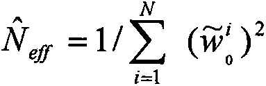 Judging whether the particle degradation degree is serious, then resampling from the obtained posterior density to obtain M new particles, and repeatingEndowing each particle with the same weight
(e) Calculating the nonlinear state quantity estimated value:
and (4) returning to the step (2), and recursively calculating the state estimation value at the next moment according to the new observed quantity.
5. The autonomous combined navigation system according to claim 2, characterized in that: the fuzzy robust adaptive particle filtering comprises the steps of constructing equivalent weights and a specific algorithm based on a fuzzy theory, wherein:
(I) constructing equivalence weight based on fuzzy theory: dividing the weight according to the data residual error into: a weight-preserving area (keeping the original observed value unchanged), a weight-reducing area (making robust limitation on the observed value) and a rejecting area (the weight is zero); designing a one-dimensional fuzzy controller, and constructing a weight factor gamma by the following steps:
(a) fuzzification: will input quantity (exact value) fuzzification becomes a fuzzy variable (where
 As normalized residual), the determined inputs are converted into a fuzzy set described by membership; the specific process comprises the following steps: will input variable
 Is divided into { too large, normal }, abbreviated as { B }e,Bc,BnAnd after the input is quantized,
 x ═ 0, 1, 2, 3, 4 }; the fuzzy subset of the output gamma is { minimal, small, normal }, abbreviated as { S }e,Sc,SnY size is divided into 5 levels to represent different values, i.e., Y ═ 0, 1, 2, 3, 4; are respectively input to
 And outputting gamma for fuzzy quantization;
(b) based on human intuition, thinking, reasoning and practical experience Designing a fuzzy control rule according to the relation between the output quantity weight factor gamma; if it is not
 If too large, γ is extremely small; if it is not
 Larger, γ is smaller; if it is not
 Normal, then gamma is normal; according to the fuzzy rule, the fuzzy relation can be determined as
R=(Be×Se)+(Bc×Sc)+(Bn×Sn);
Wherein "×" represents the cartesian product of the blur vectors; is calculated by
(c) According to fuzzy control principle, from input variables The fuzzy subset and the fuzzy relation matrix R obtain a fuzzy set with a weight factor gamma through fuzzy reasoning to obtain final fuzzy control quantity;
(d) carrying out deblurring on the fuzzy control quantity to obtain an accurate output control quantity, namely a weight factor gamma; the process of converting the fuzzy reasoning result into an accurate value is called defuzzification; in the defuzzification processing process, a maximum membership principle is adopted;
(II) the fuzzy robust adaptive particle filtering algorithm comprises the following steps:
(a) initialization: at the time k =0, N particles are sampled according to the emphasis density, and it is assumed that each sampled particle is used Let k = 1;
(b) and constructing error discrimination statistics and adaptive factors of the state model by taking the prediction residual as a variable: the discrimination statistic of the error of the state model constructed by taking the prediction residual as a variable is as follows:
wherein, predict information for the ith state at time k by
 Calculating;
 representing prediction residual
 The covariance matrix of (a); tr (-) is a matrix trace-solving operator; the adaptive factor function based on the prediction residual discrimination statistic is:
in the formula, denotes the ith adaptive factor at time k, and c is an empirical constant, generally taken to be 1.0<c<2.5;
(c) Updating:
by Updating the particle at time k according to equation (42)
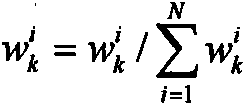
(d) resampling: sorting the weights of all the particles according to a descending order, and setting the number of threshold sample points as Nth(usually N/2 or N/3 can be selected), the number of effective sample points is NeffWhen N is presenteff<NthThen, to the particle setResampling to obtain new particle set And reset the weight value to
(e) Filtering:
and (b) calculating the filtering density at the time k, re-sampling the filtering density, making k equal to k +1, and returning.
6. The autonomous combined navigation system according to claim 2, characterized in that: the self-adaptive SVD-UKF filtering algorithm comprises the following steps:
(I) singular value decomposition: singular value decomposition is defined as follows:
assuming A ∈ Rm×n(m.gtoreq.n), the singular value decomposition of the matrix A can be expressed as
In the formula, U is belonged to Rm×m,Λ∈Rm×m,V∈Rn×n,S=diag(s1,s2,...,sr);s1≥s2≥…≥srMore than or equal to 0 is called as singular value of the matrix A, and the column vectors of U and V are respectively called as left and right singular vectors of the matrix A;
(II) determination of statistics and adaptive factors: and constructing error discrimination statistics and adaptive factors of the state model by taking the prediction residual as a variable. Prediction residualExpressed as:
in the formula, predicting information for the state at time k; using prediction residuals
 The constructed state model error discrimination statistic is as follows:
in the formula, representing prediction residual
 Tr (-) is a matrix trace-solving operator;
the adaptive factor function is selected as:
in the formula, alphakDenotes the adaptation factor, c is an empirical constant, typically 1<c<2.5;
(III) the steps of the self-adaptive SVD-UKF algorithm are as follows:
(a) initialization: initializing parameters in a state equation and calculating weight coefficients w of Sigma point mean and covariance(m)、w(c)(ii) a (b) Singular value decomposition, calculationA Sigma point vector; (c) updating the time; (d) and (6) updating the measurement.
7. The autonomous combined navigation system according to claim 2, characterized in that: the adaptive square root Unscented particle filter comprises the following steps:
(a) initialization (k = 0): randomly extracting N initial particles(i =1, 2, …, N). Suppose that Wherein, and
and respectively representing the ith particle at the initial time and the estimated value thereof,
 represents the ith Cholesky factorization at the initial time,
 the initialization weight of the ith particle is represented, and chol {. cndot } represents a Cholesky decomposition operator of the matrix;
(b) updating each particle by adopting adaptive square root UKF filtering algorithm To obtain
 Representing the covariance of the ith particle at time k, as follows:
(b1) calculating Sigma points and weight:
(b2) constructing error discrimination statistics and adaptive factors of a state model by taking the prediction residual as a variable;
the prediction residual (or innovation) contains the state which is not corrected by the observed information, and can reflect the disturbance of a dynamic system better. Ith prediction residual vector at time k Expressed as:
the discrimination statistic of the error of the state model constructed by taking the prediction residual as a variable is as follows:
wherein, predict information for the ith state at time k byThe determination is carried out by the following steps,
 representing prediction residual
 Tr (-) is a matrix trace-solving operator;
the adaptive factor function based on the prediction residual discrimination statistic is:
in the formula, denotes the ith adaptive factor at time k, and c is an empirical constant, generally taken to be 1.0<c<2.5;
(b3) Time update (state prediction);
(b4) measurement update (state estimation): QR decomposition and Cholesky decomposition in linear algebra are used in the step, and the state covariance matrix is directly propagated and updated in the form of Cholesky decomposition factors, so that the numerical stability in the updating process of the state covariance matrix is enhanced, and the positive nature of the covariance matrix is ensured;
(c) calculating importance sampling weight: let importance distribute function Sampling particles
 N (-) represents a normal distribution; respectively pass through
 <math>
<mrow>
<msubsup>
<mi>w</mi>
<mi>k</mi>
<mi>i</mi>
</msubsup>
<mo>=</mo>
<msubsup>
<mi>w</mi>
<mrow>
<mi>k</mi>
<mo>-</mo>
<mn>1</mn>
</mrow>
<mi>i</mi>
</msubsup>
<mfrac>
<mrow>
<mi>p</mi>
<mrow>
<mo>(</mo>
<msub>
<mi>Y</mi>
<mi>k</mi>
</msub>
<mo>/</mo>
<msubsup>
<mi>X</mi>
<mi>k</mi>
<mi>i</mi>
</msubsup>
<mo>)</mo>
</mrow>
<mi>p</mi>
<mrow>
<mo>(</mo>
<msubsup>
<mi>X</mi>
<mi>k</mi>
<mi>i</mi>
</msubsup>
<mo>/</mo>
<msubsup>
<mi>X</mi>
<mrow>
<mi>k</mi>
<mo>-</mo>
<mn>1</mn>
</mrow>
<mi>i</mi>
</msubsup>
<mo>)</mo>
</mrow>
</mrow>
<mrow>
<mi>q</mi>
<mrow>
<mo>(</mo>
<msubsup>
<mover>
<mi>X</mi>
<mo>‾</mo>
</mover>
<mi>k</mi>
<mi>i</mi>
</msubsup>
<mo>|</mo>
<msubsup>
<mover>
<mi>X</mi>
<mo>‾</mo>
</mover>
<mrow>
<mn>0</mn>
<mo>:</mo>
<mi>k</mi>
<mo>-</mo>
<mn>1</mn>
</mrow>
<mi>i</mi>
</msubsup>
<mo>,</mo>
<msub>
<mi>Y</mi>
<mrow>
<mn>1</mn>
<mo>:</mo>
<mi>k</mi>
</mrow>
</msub>
<mo>)</mo>
</mrow>
</mrow>
</mfrac>
<mo>,</mo>
</mrow>
</math>  Updating the weight value and the normalized weight value, wherein i is 1, … and N;
(d) resampling: setting the number of threshold sample points to Nth(usually N/2 or N/3) as the choice), valid samplesNumber of points is NeffWhen N is presenteff<NthThen, to the particle set Resampling to obtain new particle set
 And reset the weight value to
(e) And (3) updating the state: <math>
<mrow>
<msub>
<mover>
<mi>X</mi>
<mo>^</mo>
</mover>
<mi>k</mi>
</msub>
<mo>=</mo>
<munderover>
<mi>Σ</mi>
<mrow>
<mi>i</mi>
<mo>=</mo>
<mn>1</mn>
</mrow>
<mi>N</mi>
</munderover>
<msubsup>
<mover>
<mi>X</mi>
<mo>~</mo>
</mover>
<mi>k</mi>
<mi>i</mi>
</msubsup>
<msubsup>
<mover>
<mi>w</mi>
<mo>~</mo>
</mover>
<mi>k</mi>
<mi>i</mi>
</msubsup>
<mo>;</mo>
<msub>
<mover>
<mi>Σ</mi>
<mo>^</mo>
</mover>
<mi>k</mi>
</msub>
<mo>=</mo>
<munderover>
<mi>Σ</mi>
<mrow>
<mi>i</mi>
<mo>=</mo>
<mn>1</mn>
</mrow>
<mi>N</mi>
</munderover>
<msubsup>
<mover>
<mi>w</mi>
<mo>~</mo>
</mover>
<mi>k</mi>
<mi>i</mi>
</msubsup>
<mrow>
<mo>(</mo>
<msub>
<mover>
<mi>X</mi>
<mo>^</mo>
</mover>
<mi>k</mi>
</msub>
<mo>-</mo>
<msubsup>
<mover>
<mi>X</mi>
<mo>~</mo>
</mover>
<mi>k</mi>
<mi>i</mi>
</msubsup>
<mo>)</mo>
</mrow>
<msup>
<mrow>
<mo>(</mo>
<msub>
<mover>
<mi>X</mi>
<mo>^</mo>
</mover>
<mi>k</mi>
</msub>
<mo>-</mo>
<msubsup>
<mover>
<mi>X</mi>
<mo>~</mo>
</mover>
<mi>k</mi>
<mi>i</mi>
</msubsup>
<mo>)</mo>
</mrow>
<mi>T</mi>
</msup>
<mo>.</mo>
</mrow>
</math>
Priority Applications (1)
| Application Number | Priority Date | Filing Date | Title |
|---|---|---|---|
| CN201310502827.8A CN103528587B (en) | 2013-10-15 | 2013-10-15 | Independent combined navigation system |
Applications Claiming Priority (1)
| Application Number | Priority Date | Filing Date | Title |
|---|---|---|---|
| CN201310502827.8A CN103528587B (en) | 2013-10-15 | 2013-10-15 | Independent combined navigation system |
Publications (2)
| Publication Number | Publication Date |
|---|---|
| CN103528587A true CN103528587A (en) | 2014-01-22 |
| CN103528587B CN103528587B (en) | 2016-09-28 |
Family
ID=49930786
Family Applications (1)
| Application Number | Title | Priority Date | Filing Date |
|---|---|---|---|
| CN201310502827.8A Expired - Fee Related CN103528587B (en) | 2013-10-15 | 2013-10-15 | Independent combined navigation system |
Country Status (1)
| Country | Link |
|---|---|
| CN (1) | CN103528587B (en) |
Cited By (48)
| Publication number | Priority date | Publication date | Assignee | Title |
|---|---|---|---|---|
| CN104035110A (en) * | 2014-06-30 | 2014-09-10 | 北京理工大学 | Quick Kalman filtering positioning method applied to multimode satellite navigation system |
| CN104764449A (en) * | 2015-04-23 | 2015-07-08 | 北京航空航天大学 | Ephemeris correction-based autonomous celestial navigation method for deep space probe in capturing stage |
| CN104778376A (en) * | 2015-05-04 | 2015-07-15 | 哈尔滨工业大学 | A jump trajectory prediction method for hypersonic glide warhead in near space |
| CN104820648A (en) * | 2015-04-16 | 2015-08-05 | 中国电子科技集团公司第三十八研究所 | Agent-based synthetic aperture radar inertial navigation data input method and inertial navigation data input agent module |
| CN104864869A (en) * | 2015-06-05 | 2015-08-26 | 中国电子科技集团公司第二十六研究所 | Method for determining initial dynamic posture of carrier |
| CN105222772A (en) * | 2015-09-17 | 2016-01-06 | 泉州装备制造研究所 | A kind of high-precision motion track detection system based on Multi-source Information Fusion |
| CN105716610A (en) * | 2016-01-28 | 2016-06-29 | 北京航空航天大学 | Carrier attitude and heading calculation method assisted by geomagnetic field model and system |
| CN105717483A (en) * | 2016-02-06 | 2016-06-29 | 北京邮电大学 | Position determining method and device based on multisource positioning mode |
| CN105758401A (en) * | 2016-05-14 | 2016-07-13 | 中卫物联成都科技有限公司 | Integrated navigation method and equipment based on multisource information fusion |
| CN106403959A (en) * | 2016-11-22 | 2017-02-15 | 天津海运职业学院 | Electromagnetic positioning system adopting multi-sensor array |
| CN106484980A (en) * | 2016-09-29 | 2017-03-08 | 中国人民解放军军械工程学院 | A kind of fixing rudder two dimension Correction Projectiles aerodynamic coefficient method |
| CN106931967A (en) * | 2017-02-28 | 2017-07-07 | 西北工业大学 | A kind of strapdown inertial navigation method of boosting gliding type near space vehicle |
| CN107132542A (en) * | 2017-05-02 | 2017-09-05 | 北京理工大学 | A kind of small feature loss soft landing autonomic air navigation aid based on optics and Doppler radar |
| CN107577238A (en) * | 2017-08-25 | 2018-01-12 | 深圳禾苗通信科技有限公司 | The height control method of unmanned plane barometer dealing of abnormal data based on UKF |
| CN107861143A (en) * | 2017-10-31 | 2018-03-30 | 太原理工大学 | A kind of BDS/WLAN integrated positioning algorithms |
| CN108226887A (en) * | 2018-01-23 | 2018-06-29 | 哈尔滨工程大学 | A kind of waterborne target rescue method for estimating state in the case of observed quantity transient loss |
| CN108536163A (en) * | 2018-03-15 | 2018-09-14 | 南京航空航天大学 | A kind of kinetic model/laser radar Combinated navigation method under single-sided structure environment |
| CN108562289A (en) * | 2018-06-07 | 2018-09-21 | 南京航空航天大学 | Quadrotor laser radar air navigation aid in continuous polygon geometry environment |
| CN108646277A (en) * | 2018-05-03 | 2018-10-12 | 山东省计算中心(国家超级计算济南中心) | The Beidou navigation method adaptively merged with Extended Kalman filter based on robust |
| CN108663051A (en) * | 2018-04-28 | 2018-10-16 | 南京信息工程大学 | A kind of modeling of passive integrated navigation system and information fusion method under water |
| CN108731667A (en) * | 2017-04-14 | 2018-11-02 | 百度在线网络技术(北京)有限公司 | The method and apparatus of speed and pose for determining automatic driving vehicle |
| CN108803609A (en) * | 2018-06-11 | 2018-11-13 | 苏州大学 | Based on the partially observable automatic Pilot decision-making technique and system for constraining in line gauge stroke |
| CN108896036A (en) * | 2018-05-09 | 2018-11-27 | 中国人民解放军国防科技大学 | An Adaptive Federated Filtering Method Based on Innovation Estimation |
| CN108931249A (en) * | 2018-07-18 | 2018-12-04 | 兰州交通大学 | Navigation methods and systems based on the SVD Kalman filter model simplified |
| CN109115209A (en) * | 2018-07-20 | 2019-01-01 | 湖南格纳微信息科技有限公司 | Personnel positioning method and device in a kind of piping lane |
| CN109459019A (en) * | 2018-12-21 | 2019-03-12 | 哈尔滨工程大学 | A kind of vehicle mounted guidance calculation method based on cascade adaptive robust federated filter |
| CN109840643A (en) * | 2017-11-24 | 2019-06-04 | 北京自动化控制设备研究所 | A kind of performance estimating method of complex navigation blending algorithm |
| CN110160522A (en) * | 2019-04-16 | 2019-08-23 | 浙江大学 | A kind of position and orientation estimation method of the vision inertial navigation odometer based on sparse features method |
| CN110632634A (en) * | 2019-09-24 | 2019-12-31 | 东南大学 | An Optimal Data Fusion Method for Ballistic Missile INS/CNS/GNSS Integrated Navigation System |
| CN111381608A (en) * | 2020-03-31 | 2020-07-07 | 成都飞机工业(集团)有限责任公司 | Digital guiding method and system for ground directional antenna |
| CN112068092A (en) * | 2020-08-31 | 2020-12-11 | 西安工业大学 | A Robust Weighted Observation Fusion Square Root UKF Filtering Method for High Precision Ballistic Real-time Orbit Determination |
| CN112082551A (en) * | 2020-09-17 | 2020-12-15 | 蓝箭航天空间科技股份有限公司 | Navigation system capable of recycling space carrier |
| CN110187306B (en) * | 2019-04-16 | 2021-01-08 | 浙江大学 | TDOA-PDR-MAP fusion positioning method applied to complex indoor space |
| CN112461511A (en) * | 2020-11-10 | 2021-03-09 | 中国科学院长春光学精密机械与物理研究所 | Method, device and equipment for acquiring pointing direction of floating platform telescope and storage medium |
| CN112762928A (en) * | 2020-12-23 | 2021-05-07 | 重庆邮电大学 | ODOM and DM landmark combined mobile robot containing laser SLAM and navigation method |
| CN113310487A (en) * | 2021-05-25 | 2021-08-27 | 云南电网有限责任公司电力科学研究院 | Ground-oriented mobile robot-oriented integrated navigation method and device |
| CN113791432A (en) * | 2021-08-18 | 2021-12-14 | 哈尔滨工程大学 | A Combined Navigation and Positioning Method to Improve AIS Positioning Accuracy |
| CN114413932A (en) * | 2022-01-03 | 2022-04-29 | 中国电子科技集团公司第二十研究所 | Positioning error correction test method based on communication between vehicle-mounted platforms |
| CN114488224A (en) * | 2021-12-24 | 2022-05-13 | 西南交通大学 | An Adaptive Filtering Method for Satellite Centralized Autonomous Navigation |
| CN114510076A (en) * | 2022-02-10 | 2022-05-17 | 中国人民解放军战略支援部队信息工程大学 | Target cooperative detection and guidance integration method and system based on unscented transformation |
| CN114543799A (en) * | 2022-03-31 | 2022-05-27 | 湖南大学无锡智能控制研究院 | Robust federated Kalman filtering method, device and system |
| US11371846B2 (en) | 2019-01-14 | 2022-06-28 | Qatar Foundation For Education Science And Community Development | Systems and methods for determining the position of a device |
| CN115291523A (en) * | 2022-08-31 | 2022-11-04 | 东南大学 | A robust adaptive UFastSLAM autonomous navigation method based on KLD resampling |
| CN115560763A (en) * | 2022-09-24 | 2023-01-03 | 东南大学 | Elastic navigation interactive information fusion method based on robust estimation |
| CN115855021A (en) * | 2022-11-24 | 2023-03-28 | 北京宇航系统工程研究所 | A SINS/CNS/SAR Integrated Navigation Method Based on Multigroup Cooperative PF Algorithm |
| CN116255988A (en) * | 2023-05-11 | 2023-06-13 | 北京航空航天大学 | A Composite Anti-jamming Adaptive Filtering Method Based on Ship Dynamics Integrated Navigation |
| CN117647251A (en) * | 2024-01-30 | 2024-03-05 | 山东科技大学 | A robust adaptive integrated navigation method based on observation noise covariance matrix |
| CN119915296A (en) * | 2025-01-24 | 2025-05-02 | 西安理工大学 | A distributed spectral redshift/starlight refraction combined navigation method and related products |
Citations (1)
| Publication number | Priority date | Publication date | Assignee | Title |
|---|---|---|---|---|
| CN101270993A (en) * | 2007-12-12 | 2008-09-24 | 北京航空航天大学 | A long-distance high-precision autonomous integrated navigation and positioning method |
-
2013
- 2013-10-15 CN CN201310502827.8A patent/CN103528587B/en not_active Expired - Fee Related
Patent Citations (1)
| Publication number | Priority date | Publication date | Assignee | Title |
|---|---|---|---|---|
| CN101270993A (en) * | 2007-12-12 | 2008-09-24 | 北京航空航天大学 | A long-distance high-precision autonomous integrated navigation and positioning method |
Non-Patent Citations (7)
| Title |
|---|
| 薛丽等: "一种新的抗差自适应Unscented粒子滤波", 《西北工业大学学报》 * |
| 高社生等: "抗差自适应模型预测滤波及其在组合导航中的应用", 《中国惯性技术学报》 * |
| 高社生等: "抗差自适应模型预测滤波及其在组合导航中的应用", 《中国惯性技术学报》, vol. 19, no. 6, 31 December 2011 (2011-12-31) * |
| 高社生等: "模糊抗差自适应粒子滤波及其在组合导航中的应用", 《中国惯性技术学报》 * |
| 高社生等: "渐消自适应 Unscented 粒子滤波及其在组合导航中的应用", 《西北工业大学学报》 * |
| 高社生等: "自适应SVD-UKF算法及在组合导航的应用", 《中国惯性技术学报》 * |
| 高社生等: "自适应平方根Unscented粒子滤波算法研究", 《西北工业大学学报》 * |
Cited By (72)
| Publication number | Priority date | Publication date | Assignee | Title |
|---|---|---|---|---|
| CN104035110A (en) * | 2014-06-30 | 2014-09-10 | 北京理工大学 | Quick Kalman filtering positioning method applied to multimode satellite navigation system |
| CN104035110B (en) * | 2014-06-30 | 2016-08-17 | 北京理工大学 | The Fast Kalman filtering localization method being applied in multimodal satellite navigation system |
| CN104820648A (en) * | 2015-04-16 | 2015-08-05 | 中国电子科技集团公司第三十八研究所 | Agent-based synthetic aperture radar inertial navigation data input method and inertial navigation data input agent module |
| CN104820648B (en) * | 2015-04-16 | 2018-04-06 | 中国电子科技集团公司第三十八研究所 | A kind of synthetic aperture radar inertial guidance data input method and input agency plant |
| CN104764449B (en) * | 2015-04-23 | 2017-07-11 | 北京航空航天大学 | A kind of capture section deep space probe celestial self-navigation method based on ephemeris amendment |
| CN104764449A (en) * | 2015-04-23 | 2015-07-08 | 北京航空航天大学 | Ephemeris correction-based autonomous celestial navigation method for deep space probe in capturing stage |
| CN104778376A (en) * | 2015-05-04 | 2015-07-15 | 哈尔滨工业大学 | A jump trajectory prediction method for hypersonic glide warhead in near space |
| CN104778376B (en) * | 2015-05-04 | 2018-03-16 | 哈尔滨工业大学 | Method for predicting jumping trajectory of hypersonic gliding warhead in near space |
| CN104864869A (en) * | 2015-06-05 | 2015-08-26 | 中国电子科技集团公司第二十六研究所 | Method for determining initial dynamic posture of carrier |
| CN104864869B (en) * | 2015-06-05 | 2017-11-21 | 中国电子科技集团公司第二十六研究所 | A kind of initial dynamic attitude determination method of carrier |
| CN105222772A (en) * | 2015-09-17 | 2016-01-06 | 泉州装备制造研究所 | A kind of high-precision motion track detection system based on Multi-source Information Fusion |
| CN105222772B (en) * | 2015-09-17 | 2018-03-16 | 泉州装备制造研究所 | A kind of high-precision motion track detection system based on Multi-source Information Fusion |
| CN105716610A (en) * | 2016-01-28 | 2016-06-29 | 北京航空航天大学 | Carrier attitude and heading calculation method assisted by geomagnetic field model and system |
| CN105717483A (en) * | 2016-02-06 | 2016-06-29 | 北京邮电大学 | Position determining method and device based on multisource positioning mode |
| CN105717483B (en) * | 2016-02-06 | 2019-01-25 | 北京邮电大学 | A method and device for determining a position based on a multi-source positioning method |
| CN105758401A (en) * | 2016-05-14 | 2016-07-13 | 中卫物联成都科技有限公司 | Integrated navigation method and equipment based on multisource information fusion |
| CN106484980A (en) * | 2016-09-29 | 2017-03-08 | 中国人民解放军军械工程学院 | A kind of fixing rudder two dimension Correction Projectiles aerodynamic coefficient method |
| CN106484980B (en) * | 2016-09-29 | 2019-08-13 | 中国人民解放军军械工程学院 | A kind of fixed rudder two dimension Correction Projectiles aerodynamic coefficient method |
| CN106403959A (en) * | 2016-11-22 | 2017-02-15 | 天津海运职业学院 | Electromagnetic positioning system adopting multi-sensor array |
| CN106931967A (en) * | 2017-02-28 | 2017-07-07 | 西北工业大学 | A kind of strapdown inertial navigation method of boosting gliding type near space vehicle |
| CN106931967B (en) * | 2017-02-28 | 2019-10-18 | 西北工业大学 | A Strapdown Inertial Navigation Method for Boost-Glide Near-Space Vehicle |
| CN108731667B (en) * | 2017-04-14 | 2020-09-29 | 百度在线网络技术(北京)有限公司 | Method and apparatus for determining speed and pose of unmanned vehicle |
| CN108731667A (en) * | 2017-04-14 | 2018-11-02 | 百度在线网络技术(北京)有限公司 | The method and apparatus of speed and pose for determining automatic driving vehicle |
| CN107132542B (en) * | 2017-05-02 | 2019-10-15 | 北京理工大学 | An autonomous navigation method for small celestial body soft landing based on optical and Doppler radar |
| CN107132542A (en) * | 2017-05-02 | 2017-09-05 | 北京理工大学 | A kind of small feature loss soft landing autonomic air navigation aid based on optics and Doppler radar |
| CN107577238A (en) * | 2017-08-25 | 2018-01-12 | 深圳禾苗通信科技有限公司 | The height control method of unmanned plane barometer dealing of abnormal data based on UKF |
| CN107577238B (en) * | 2017-08-25 | 2020-12-18 | 深圳禾苗通信科技有限公司 | UKF-based height control method for processing abnormal data of unmanned aerial vehicle barometer |
| CN107861143A (en) * | 2017-10-31 | 2018-03-30 | 太原理工大学 | A kind of BDS/WLAN integrated positioning algorithms |
| CN109840643B (en) * | 2017-11-24 | 2021-05-11 | 北京自动化控制设备研究所 | A Performance Evaluation Method for Composite Navigation Fusion Algorithm |
| CN109840643A (en) * | 2017-11-24 | 2019-06-04 | 北京自动化控制设备研究所 | A kind of performance estimating method of complex navigation blending algorithm |
| CN108226887A (en) * | 2018-01-23 | 2018-06-29 | 哈尔滨工程大学 | A kind of waterborne target rescue method for estimating state in the case of observed quantity transient loss |
| CN108226887B (en) * | 2018-01-23 | 2021-06-01 | 哈尔滨工程大学 | Water surface target rescue state estimation method under condition of transient observation loss |
| CN108536163A (en) * | 2018-03-15 | 2018-09-14 | 南京航空航天大学 | A kind of kinetic model/laser radar Combinated navigation method under single-sided structure environment |
| CN108663051A (en) * | 2018-04-28 | 2018-10-16 | 南京信息工程大学 | A kind of modeling of passive integrated navigation system and information fusion method under water |
| CN108646277A (en) * | 2018-05-03 | 2018-10-12 | 山东省计算中心(国家超级计算济南中心) | The Beidou navigation method adaptively merged with Extended Kalman filter based on robust |
| CN108896036B (en) * | 2018-05-09 | 2021-01-22 | 中国人民解放军国防科技大学 | An Adaptive Federal Filtering Method Based on Innovation Estimation |
| CN108896036A (en) * | 2018-05-09 | 2018-11-27 | 中国人民解放军国防科技大学 | An Adaptive Federated Filtering Method Based on Innovation Estimation |
| CN108562289A (en) * | 2018-06-07 | 2018-09-21 | 南京航空航天大学 | Quadrotor laser radar air navigation aid in continuous polygon geometry environment |
| CN108803609B (en) * | 2018-06-11 | 2020-05-01 | 苏州大学 | Partially observable decision-making method for autonomous driving based on constrained online programming |
| CN108803609A (en) * | 2018-06-11 | 2018-11-13 | 苏州大学 | Based on the partially observable automatic Pilot decision-making technique and system for constraining in line gauge stroke |
| CN108931249A (en) * | 2018-07-18 | 2018-12-04 | 兰州交通大学 | Navigation methods and systems based on the SVD Kalman filter model simplified |
| CN109115209B (en) * | 2018-07-20 | 2022-03-11 | 湖南格纳微信息科技有限公司 | Method and device for positioning personnel in pipe gallery |
| CN109115209A (en) * | 2018-07-20 | 2019-01-01 | 湖南格纳微信息科技有限公司 | Personnel positioning method and device in a kind of piping lane |
| CN109459019A (en) * | 2018-12-21 | 2019-03-12 | 哈尔滨工程大学 | A kind of vehicle mounted guidance calculation method based on cascade adaptive robust federated filter |
| US11371846B2 (en) | 2019-01-14 | 2022-06-28 | Qatar Foundation For Education Science And Community Development | Systems and methods for determining the position of a device |
| CN110187306B (en) * | 2019-04-16 | 2021-01-08 | 浙江大学 | TDOA-PDR-MAP fusion positioning method applied to complex indoor space |
| CN110160522A (en) * | 2019-04-16 | 2019-08-23 | 浙江大学 | A kind of position and orientation estimation method of the vision inertial navigation odometer based on sparse features method |
| CN110632634A (en) * | 2019-09-24 | 2019-12-31 | 东南大学 | An Optimal Data Fusion Method for Ballistic Missile INS/CNS/GNSS Integrated Navigation System |
| CN111381608A (en) * | 2020-03-31 | 2020-07-07 | 成都飞机工业(集团)有限责任公司 | Digital guiding method and system for ground directional antenna |
| CN112068092A (en) * | 2020-08-31 | 2020-12-11 | 西安工业大学 | A Robust Weighted Observation Fusion Square Root UKF Filtering Method for High Precision Ballistic Real-time Orbit Determination |
| CN112068092B (en) * | 2020-08-31 | 2023-03-17 | 西安工业大学 | Robust weighted observation fusion square root UKF filtering method for high-precision trajectory real-time orbit determination |
| CN112082551A (en) * | 2020-09-17 | 2020-12-15 | 蓝箭航天空间科技股份有限公司 | Navigation system capable of recycling space carrier |
| CN112461511B (en) * | 2020-11-10 | 2022-03-25 | 中国科学院长春光学精密机械与物理研究所 | Method, device and equipment for acquiring pointing direction of floating platform telescope and storage medium |
| CN112461511A (en) * | 2020-11-10 | 2021-03-09 | 中国科学院长春光学精密机械与物理研究所 | Method, device and equipment for acquiring pointing direction of floating platform telescope and storage medium |
| CN112762928A (en) * | 2020-12-23 | 2021-05-07 | 重庆邮电大学 | ODOM and DM landmark combined mobile robot containing laser SLAM and navigation method |
| CN112762928B (en) * | 2020-12-23 | 2022-07-15 | 重庆邮电大学 | ODOM and DM landmark combined mobile robot containing laser SLAM and navigation method |
| CN113310487A (en) * | 2021-05-25 | 2021-08-27 | 云南电网有限责任公司电力科学研究院 | Ground-oriented mobile robot-oriented integrated navigation method and device |
| CN113791432A (en) * | 2021-08-18 | 2021-12-14 | 哈尔滨工程大学 | A Combined Navigation and Positioning Method to Improve AIS Positioning Accuracy |
| CN114488224A (en) * | 2021-12-24 | 2022-05-13 | 西南交通大学 | An Adaptive Filtering Method for Satellite Centralized Autonomous Navigation |
| CN114413932B (en) * | 2022-01-03 | 2024-05-14 | 中国电子科技集团公司第二十研究所 | Positioning error correction testing method based on communication between vehicle-mounted platforms |
| CN114413932A (en) * | 2022-01-03 | 2022-04-29 | 中国电子科技集团公司第二十研究所 | Positioning error correction test method based on communication between vehicle-mounted platforms |
| CN114510076A (en) * | 2022-02-10 | 2022-05-17 | 中国人民解放军战略支援部队信息工程大学 | Target cooperative detection and guidance integration method and system based on unscented transformation |
| CN114510076B (en) * | 2022-02-10 | 2025-04-01 | 中国人民解放军网络空间部队信息工程大学 | Integrated method and system for target cooperative detection and guidance based on traceless transformation |
| CN114543799A (en) * | 2022-03-31 | 2022-05-27 | 湖南大学无锡智能控制研究院 | Robust federated Kalman filtering method, device and system |
| CN114543799B (en) * | 2022-03-31 | 2023-10-27 | 湖南大学无锡智能控制研究院 | A robust federated Kalman filtering method, equipment and system |
| CN115291523A (en) * | 2022-08-31 | 2022-11-04 | 东南大学 | A robust adaptive UFastSLAM autonomous navigation method based on KLD resampling |
| CN115291523B (en) * | 2022-08-31 | 2025-07-18 | 东南大学 | Robust self-adaptive UFastSLAM autonomous navigation method based on KLD resampling |
| CN115560763A (en) * | 2022-09-24 | 2023-01-03 | 东南大学 | Elastic navigation interactive information fusion method based on robust estimation |
| CN115855021A (en) * | 2022-11-24 | 2023-03-28 | 北京宇航系统工程研究所 | A SINS/CNS/SAR Integrated Navigation Method Based on Multigroup Cooperative PF Algorithm |
| CN116255988A (en) * | 2023-05-11 | 2023-06-13 | 北京航空航天大学 | A Composite Anti-jamming Adaptive Filtering Method Based on Ship Dynamics Integrated Navigation |
| CN117647251A (en) * | 2024-01-30 | 2024-03-05 | 山东科技大学 | A robust adaptive integrated navigation method based on observation noise covariance matrix |
| CN119915296A (en) * | 2025-01-24 | 2025-05-02 | 西安理工大学 | A distributed spectral redshift/starlight refraction combined navigation method and related products |
Also Published As
| Publication number | Publication date |
|---|---|
| CN103528587B (en) | 2016-09-28 |
Similar Documents
| Publication | Publication Date | Title |
|---|---|---|
| CN103528587B (en) | Independent combined navigation system | |
| Hu et al. | Model predictive based unscented Kalman filter for hypersonic vehicle navigation with INS/GNSS integration | |
| Li et al. | A machine learning-based approach for improved orbit predictions of LEO space debris with sparse tracking data from a single station | |
| Wang et al. | Huber-based unscented filtering and its application to vision-based relative navigation | |
| Qiu et al. | Outlier-robust extended Kalman filtering for bioinspired integrated navigation system | |
| Soken et al. | UKF-based reconfigurable attitude parameters estimation and magnetometer calibration | |
| US20120022784A1 (en) | Navigation filter for a navigation system using terrain correlation | |
| CN106197408A (en) | A kind of multi-source navigation data fusion method based on factor graph | |
| WO2020085412A1 (en) | Prediction device, prediction method, and prediction program | |
| Rhudy et al. | Sensitivity analysis of extended and unscented Kalman filters for attitude estimation | |
| CN115420280B (en) | A spacecraft pulsar/starlight refraction combined navigation method | |
| Sabatini et al. | Carrier-phase GNSS attitude determination and control system for unmanned aerial vehicle applications | |
| Gao et al. | SIMU/Triple star sensors integrated navigation method of HALE UAV based on atmospheric refraction correction | |
| CN115097438A (en) | High-precision space target tracking method based on adaptive unscented Kalman filtering | |
| CN117842386B (en) | An Adaptive Calibration Method for Orbit Control Thrust Based on Inter-Satellite Distance and Error Compensation | |
| Dai et al. | An improved gaussian sum extended Kalman filter with colored noise for GNSS/SINS tightly coupled positioning and attitude determination systems | |
| Chen et al. | Spacecraft autonomous GPS navigation based on polytopic linear differential inclusion | |
| CN114993341A (en) | Carrier rocket trajectory estimation method and device based on space-based measurement | |
| CN113324539A (en) | SINS/SRS/CNS multi-source fusion autonomous integrated navigation method | |
| Erkeç et al. | Fault-tolerant estimation of satellite orbital states | |
| Zhang et al. | Estimation of aerodynamic parameter for maneuvering reentry vehicle tracking | |
| Fu et al. | Adaptive Tracking Algorithm for Hypersonic Maneuvering Target Based on Bi-Satellite Positioning | |
| Xiao-Gang et al. | An orbital prediction algorithm for LEO satellites based on optical observations of short arcs at single station | |
| Zhang et al. | Improved Cubature Kalman filter algorithm based on magnetometer and gyroscope | |
| Hua et al. | Research Article Angle-Only Target Tracking Method for Optical Imaging Micro-/Nanosatellite Based on APSO-SSUKF |
Legal Events
| Date | Code | Title | Description |
|---|---|---|---|
| C06 | Publication | ||
| PB01 | Publication | ||
| C10 | Entry into substantive examination | ||
| SE01 | Entry into force of request for substantive examination | ||
| C14 | Grant of patent or utility model | ||
| GR01 | Patent grant | ||
| CF01 | Termination of patent right due to non-payment of annual fee |
Granted publication date: 20160928 Termination date: 20161015 |
|
| CF01 | Termination of patent right due to non-payment of annual fee |