CN100493001C - Automatic clustering method for multi-particle size network under G bit flow rate - Google Patents

Abstract

The invention relates to a multi-granularity network automatic clustering method under a G bit flow rate, which belongs to the technical field of computer network measurement. It is characterized by a periodic sampling mechanism based on network measurement, using a heuristic algorithm based on traffic prediction, and at the same time, by considering different fields of the IP header as different dimensions in the network feature space, it proposes automatic data processing for multi-dimensional space. Adaptive algorithms for classification. The main steps are: 1. Set relevant parameters; 2. Start the measurement program; 3. Within a measurement period, perform one-dimensional source address and destination address clustering for each arriving message in sequence, and the source/destination address team Clustering and port clustering; 4. Data compression and output; 5. Traffic prediction. Experiments show that this method can run in real time on the Internet with a Gbit rate, and achieves the expected invention goal.

Description

Multi-granularity network automatic clustering method at G bit rate

technical field

The invention relates to a multi-granularity network automatic clustering method under a G bit flow rate, which belongs to the technical field of computer network measurement.

Background technique

The Internet has become an important infrastructure of the contemporary information society. With the continuous advancement of Internet technology and the increasing trend of network convergence, more and more services on traditional telecommunication networks and television networks have been carried on IP networks; at the same time, more and more new services are emerging on the Internet itself. In particular, the emergence of peer-to-peer network P2P (peer-to-peer) has changed the development direction of the entire Internet. The Internet is changing towards ultra-high speed, mobile, large capacity, and multi-service. How to accurately measure and monitor applications based on high-speed Internet has become an urgent problem to be solved.

Cluster analysis of network traffic is the key and basic technology to realize effective network measurement. Traditional network measurement systems generally classify some specific fields of IP headers. The clustering algorithm is also different due to different requirements of management functions. For example, the clustering algorithm applied to network security detects denial of service attacks based on the aggregation of destination addresses. The disadvantage of this kind of cluster analysis method is that each measurement system focuses on one aspect of traffic cluster analysis, and cannot meet the needs of modern network management to fully grasp the network operation status. By considering different fields of IP header as different dimensions of network data, researching and proposing an adaptive algorithm for automatic clustering analysis of data points in multi-dimensional space can overcome the above-mentioned shortcomings of traditional network measurement technology. Different from traditional network clustering methods based on specific network field matching rules, this method can perform dynamic clustering through preset network status thresholds. The so-called multi-granularity has the following two meanings: 1) The measurement target includes multiple network characteristics (source, destination IP address and port number. 2) The network address level of the measurement result may be different, for example, it may be accurate to a single IP , it is also possible to be accurate to a certain subnet, as long as they all meet the preset network status, for example, the traffic sent or received exceeds a certain threshold. This measurement result conforms to the mouse-like distribution characteristic of unbalanced network traffic distribution, and provides an effective means for network administrators to diagnose the network status.

Compared with the existing research work on similar offline systems, (Estan, C., Savage, S., and Varghese, G. Automatically Inferring Patterns of Resource Consumption in Network Traffic. In Proceedings of ACM SIGCOMM, Karlsruhe, Germany, 2003, 137 -148.-This method is referred to as CP in the following experiments. This method is based on the periodic sampling mechanism of network measurement, and adopts a heuristic algorithm based on traffic prediction, which reduces the time and space overhead required by existing algorithms. Experiments show that it can run on the high-speed Internet of 1Gbit/s in real time, and the expected invention goal has been achieved.

Contents of the invention

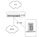
The purpose of the present invention is to provide a multi-granularity network traffic high-speed automatic clustering method. The actual deployment diagram of the present invention is shown in Fig. 3. This measurement method belongs to the passive measurement category in the field of network measurement, and forwards the network message to the server through the port mirroring function of the router or high-end switch. The actual test environment of our system is the campus network of Tsinghua University, which is a typical campus network with nearly 40,000 IP addresses. The system is deployed at the backbone exit of a campus network. In practical application, this method can be used to measure the one-way interface or the two-way interface.

The relevant data structures used in the description method are as follows:

IP address tree model: If the 32-bit IP address is hierarchically divided from high to low, the depth W of the node is the depth of the IP prefix. For example, the node ^* . ^* . ^* . ^* represents the topmost node, (also That is to say, any other address content is included in the root node, and the symbol ^* represents an address wildcard, that is to say, the address ^* . ^* . ^* . ^* can include any node), and Figure 1 shows node 1.2.3.4 and node 1.2. 3.5 address tree model. The root node of the tree, that is, the IP address " ^* . ^* . ^* . ^* ", has a node depth of 0. The child node of each tree node is the IP address of the next depth with the same prefix. For example, the child node corresponding to node 1.2.3. ^* in the address tree is "1.2.3.4, 1.2.3.5" and so on. Considering the actual needs of the network management, set the maximum level of the node to 4, that is to say, for any address, it can be located in a single address, subnet address, and the subnet belongs to the community, and the apex address ( ^* . ^* . ^* . ^* ) Four levels.

Obviously, any layer of tree nodes can be uniquely represented by the prefix of the IP address. The length of the prefix determines the depth of the node. In the case that the node level is evenly divided into 4 layers according to the IP address length, the relationship between the prefix length N of the binary IP address tree node of the node and the depth W of the IP is W=N/8.

One-dimensional tree node: the data structure in each node in the IP address tree model is as follows

Two-dimensional cross product form: as shown in Figure 4. The two dimensions of the cross product table H are the depths of the source address and the destination address respectively. And each node position stores the index table of the source address and the destination address under the depth. In the programming implementation, a two-dimensional matrix is used for storage, and each element in the matrix is a hash table. The index of the hash table is the node identification of the source address and the destination address at the current depth, and its storage content is all The current measurement value and the previous measurement value corresponding to the address depth are the initially set packet size or number of packets. For example: H[2][3] stores all node sets whose source address depth is 2 and destination address depth is 3. It may include the IP field <1.2. ^* . ^* , 3.4.5. ^* >, which indicates that the source address and destination address of the data packet are 1.2. ^* . ^* , 3.4.5. ^* in this measurement period and the packet size or number of packets obtained in the previous measurement period.

Port hash table: The port hash table P stores data information about ports, and its index IP address stores the corresponding port-capacity pairs. For example, the content stored in the table P<1, 2, 3, 4> is {(80, 125), (135, 45)}, which represents the port at the IP address 1.2.3.4 of the network packet by default. The size of the data packet transmitted by port 80 is 125 bytes, and the size of the data packet transmitted by port 135 is 45 bytes.

A note about node compression:

In order to save system space resources, the system only outputs nodes after compensation when compressing and outputting. The so-called compensation means that if a child node of a node is marked as a cluster node (the sum of the current capacity of the node and the child capacity is greater than A node with a certain threshold), then the output of the node is marked as the capacity of the node minus the capacity of all child nodes marked as clustering nodes. Obviously, if no compensation is made, then for any unclustered parent node of a child node, its current capacity must include the capacity of the child node, and these data are meaningless to network managers.

The present invention is characterized in that the proposed method contains the following steps successively (the overall flow chart is as shown in Figure 2):

Overall steps:

After the program is started, it works in the network as follows,

Step (1). Set the following parameters:

The measurement period for measuring network packets within the time interval T, T=1 minute;

The measurement target value is the packet size;

Clustering degree Phi=1%, Phi reflects the ratio of the network measurement target value of the clustering result to the current total network measurement target value, and is used to reflect the individual networks whose clustered measurement value accounts for more than 1% of the total measurement target value clustering;

Allowable value of measurement error ε, ε=1% Phi;

The total measurement target value V _cur in the current measurement period T, the measurement value V _last of the previous measurement period and the predicted value V of the next measurement period are 0;

The heuristic algorithm predicts the depth threshold T _g , the default is 0.8phi=0.008, (ε<<T _g ≤ phi), and T _g is the performance parameter of the heuristic algorithm;

Slip factor α, α=0.5;

split threshold T _split , the initial value is 0;

The maximum node depth W _max , that is, the maximum depth of the IP prefix, W _max = 4, the depth of the root node in the IP address tree model is W = 0;

Step (2) Start the measurement program, and set the total target value of the current measurement V _cur =0;

Step (3) In a measurement period T, the following steps are executed sequentially for each arriving message E:

Step (3.1) sets the one-dimensional tree storage structure, the data structure of each tree node is:

The child pointer is the child node pointer pointing to the tree node, pointing to the memory space where the child node is located, using a pointer array to represent multiple child pointers, and the initial value is empty;

The predicted depth is the depth of the node in the next measurement period, and the initial value is 0;

The actual depth is the current node depth;

Leaf attribute, if it is true, it means that the node is a leaf node, if it is false, it is false, and the initial value is false;

Current capacity, the initial message size contained in the tree node in the current measurement period, expressed in bytes;

Child node capacity, the initial message size contained in the child node of the tree node, the initial value is 0;

The previous capacity, the size of all the messages contained in the tree node in the previous measurement period, is equal to the sum of the power-saving current capacity obtained in the previous measurement period and the child node capacity, and the initial value is 0;

Step (3.2) update the one-dimensional tree storage structure according to the following steps, input the source address of the message and the measurement target value of E, and return the source address depth W1;

Step (3.2.1) setting is marked as the current node of the IP address tree root node of ^* . ^* . ^* . ^* ;

Step (3.2.2) meets any one of the following three conditions, then the current node of the step (3.2) exits:

When a leaf node appears, and its current capacity plus the measurement target value is less than the split threshold T _split , update the current node capacity value to the current measurement value plus the current node capacity, and return the predicted depth of the current node;

A leaf node appears, and its current capacity plus the measurement target value is not less than the split threshold value T _split , but its current depth has reached the maximum depth W _max , update the current node as a child node, and its capacity is the measurement target value, and return the current node Prediction depth; otherwise, set the leaf node attribute to false;

When a non-leaf node appears, its current capacity plus the measurement target value is not less than the split threshold value T _split , but its current depth is equal to the maximum depth W _max , then return the predicted depth of the current node;

If the above three exit conditions are not satisfied, no matter whether the node is a leaf node or not, the child node capacity of the current node is updated to be the child node capacity of the current node plus the measurement target value; in the above conditions, if the growth of the node capacity exceeds Split domain value T _split , but when the current depth is less than the maximum depth, the node splits a new child node according to the input IP address and the current depth and replaces the original node as the current node at the same time to continue the step (3.2.2) until the node at the maximum depth W _max ;

Step (3.3) updates the one-dimensional tree-like storage structure according to the method described in step (3.2), and the input parameter is the destination address of the message and the measurement target value of E, and returns the depth W2 of the destination address;

Step (3.4) performs the following steps respectively according to the depth of the source address and destination address returned by step (3.2) and step (3.3)

Step (34.1) If either the depth of the source address or the depth of the destination address returned is greater than 0, then obtain the IP prefix identifier at the corresponding depth according to the source address and destination address, set prefix1 and prefix2, if there is no two-dimensional cross product table In the hash index table in H[W1][W2], open up space, and initialize the measurement value to 0; otherwise, update the measurement value to the original measurement value plus the measurement target value of message E, the two-dimensional The two dimensions of the cross-product table are the depth [W1] of the source address and the depth [W2] of the destination address, and the position of each node is stored in the index table of the source address and the destination address at the depth. The table is stored in a two-dimensional matrix. Each element in the matrix is a hash table. The index in the hash table is the node identification of the source address and the destination address at the current depth; its storage content is the current measurement of the address depth The target value and the measured target value of the previous measurement cycle;

Step (3.4.2) If the depth of the returned source address or destination address is the maximum value W _max , then update the port hash table P: when the address index does not exist in P, open up the relevant space and initialize the measured value is 0; otherwise, update the port measurement value corresponding to the source address or destination address index to the original measurement value plus the measurement target value of E;

Step (3.5) increases the measurement target value of the message to the current measurement total target value V _cur , and repeats steps (3.2)-(3.4) for the next message;

Step (4) Set the current node as the root node of the source address tree and the destination address tree respectively according to the following steps, and its node identifiers are all ^* . ^* . ^* . ^* , and respectively follow the steps (4.1) to compress;

Step (4.1). If the current capacity of the current node plus the child node capacity of the current node is less than V Phi, then set the leaf attribute of the current node to be true, wherein the predicted capacity V is calculated according to step 7;

Step (4.1.1) If the sum of the current capacity of the current node and the capacity of the child node is greater than the predicted depth capacity Tg V, then update the predicted depth of the current node to be the current depth of the current node;

Step (4.1.2) If the sum of the current capacity of the current node and the child node capacity is less than Tg V, then update the current depth to be the node depth minus 1, clear the space of all its child nodes, and release related resources;

Step (4.2) If the sum of the current capacity of the current node and the child node capacity exceeds V Phi, then set the predicted depth of the current node as the current depth of the current node; for each child node of the current node, set it as the current node According to step (4.1), compress successively;

Step (5) performs the following sub-steps on the source address and the destination address respectively, and outputs the clustering results of the one-dimensional source address and the destination address, as shown in Figure 8;

Step (5.1) Set the current node V as the root node of the address tree ^* . ^* . ^* . ^* , and initialize the node queue Q to be empty; for each non-empty child node pointed to by the child pointer of node V, enter it into the queue Q ;

Step (5.2) Take out the first node V1 of the queue Q, remove V1 from the queue Q, set it as the current node, and set its compensation value T to 0;

Step (5.3) For each child of the current node V1, perform the following steps respectively, and V11 is used as an example to illustrate below;

Step (5.3.1) If the current capacity of the child node V11 and the child node capacity of the child node V11 are greater than V Phi, then increase the compensation value T to be the original capacity of T plus the current capacity of V11 and the child node capacity of V11 , and put the child node V11 into the queue Q;

Step (5.4) If the capacity of the current node V1 plus the child node capacity of the current node V1 minus the compensation value T is greater than the threshold V*Phi, output the current node V1 as a static clustering node;

Step (5.5) If the current capacity of the current node V1 plus the child node capacity of V11 minus its previous capacity is greater than the threshold V*Phi, output the current node V1 as a dynamic node;

Step (5.6) sets the previous capacity of the current node V1 to be the current capacity of V11 plus the child node capacity, and sets its current capacity to be 0; the child node capacity of V1 is set to be 0;

Step (5.7) If the queue Q is not empty, return to step (5.2) to continue, otherwise exit step (5);

Step (6) Compress and output the source-destination address pair in the cross-product table, that is, for each dimension in the cross-product table and the data item e corresponding to each hash index in the dimension, perform the following steps in turn

Step (6.1) If the absolute value of the current capacity of e minus the last capacity is greater than the threshold V _cur Phi, output e as a dynamic clustering node;

Step (6.2) If the current capacity of e is greater than V _cur Phi, the output node e is a static clustering node;

Step (6.3) If the current capacity of e is 0, delete the node and continue to execute step (6);

Step (6.4) Set the previous capacity of the node as the current capacity, set the current capacity of the node as 0, and proceed to step (6); step (7) flow forecasting, using a simple weighted exponential average model, according to the following formula Predict the next flow V;

V＝αV _cur +(1-α)V _last ，________________________(1)

Step (8). Calculate the split threshold T _split used in step 3;

T _split = ε·(phi)·V/W，____________________(2)

Step (9). Return to step (3) to enter the next measurement period.

Description of drawings

Figure 1. Schematic diagram of the address tree model;

Figure 2. Framework diagram of multi-granularity network traffic high-speed automatic clustering method;

Figure 3. Deployment diagram of multi-granularity network traffic high-speed automatic clustering method;

Figure 4. Schematic diagram of cross-product table H (Cross-product table)

X- source address depth, the value is an integer from 0 to W

Y-Destination address depth, the value is an integer from 0 to W

<prefix1, prefix2> - indicates the set of source and destination address prefixes at a specific depth.

Fig. 5. experiment measures the present invention and existing method accuracy comparison;

-□-traditional CP algorithm, please refer to the background technology for details

-O-invention (HCP) algorithm under the condition of T _g =Phi

- ^* - Invention (HCP) algorithm under the condition of T _g =0.6*Phi

Fig. 6. experiment measures the present invention and existing method time comparison;

-O-invention (HCP) algorithm under the condition of T _g =Phi

-发明(HCP)算法在T_g＝0.6*Phi条件下-

- Invention (HCP) algorithm under the condition of T _g =0.6*Phi

Figure 7. Comparison of data compression and uncompression methods

Figure 8. Schematic diagram of outputting one-dimensional address tree clustering results

Detailed ways

This algorithm is implemented in a Linux working environment with 2.4GHz CPU and 512M memory, and all codes are written in C language. The following is a further description of this experiment from different aspects. It should be noted that because the algorithm uses a heuristic algorithm, Tg=0 in the first measurement period of network packets, so network clusters cannot be correctly marked, so the experimental results need to be counted from the second measurement period.

Actual error analysis:

The correct rate analysis of this test is shown in Figure 5. It can be seen that when Phi=1% is usually taken, the error rate is kept below 2%. For different phi values, it can be performed by adjusting the threshold parameter T _g Balance between accuracy and system resources. Time performance analysis:

The analysis of the time used in this test environment is shown in Figure 6. When the measurement interval T is set to 1 minute, the time required for the measurement can be controlled within 1 minute, which can meet the line speed processing requirements.

Space performance analysis:

In this experiment, the space comparison of compressed and uncompressed data is shown in Figure 7.

Theoretical error analysis:

For the one-dimensional case, the maximum node of each cluster is ε·phi·V/W, so the error of the maximum flow of the bottom node is ε·phi·V, and its relative maximum error is ε·phi·V /(phi·V)=ε.

Error rate for this test:

1). If the predicted depth > the actual depth, that is to say, the clustering is too fine, this situation can be processed in the data compression at the end, so the error will not increase.

2). If the predicted depth < the actual depth, then there will be insufficient clustering accuracy and a false positive rate (FalsePositive). In practice, because network traffic has a relatively large correlation in a short period of time, it will not have a large impact on the accuracy of the measurement method. (See Figure 5 for specific experimental data)

It can be seen that the present invention has achieved the intended purpose.

Claims (1)

1.G the many granularities network automatic clustering method under the bit flow rate, it is characterized in that described method is to realize in a Port Mirroring function by router or high-end switch is accepted the flow detection server of message, its steps in sequence is as follows: step (1) is provided with following parameter:

The measuring period of in time interval T, network message being measured, T=1 minute;

The measurement target value is message size;

Cluster degree Phi=1%, the network measure desired value of Phi reflection cluster result accounts for the ratio of the measurement target value of current overall network, accounts for overall measurement desired value each network clustering more than 1% in order to the measured value that reflects the single network cluster;

Measure error permissible value ε, ε=1%Phi;

Overall measurement desired value V in the current measurement period T _Cur, last time measuring period measured value V _LastV is 0 with lower whorl predicted value measuring period;

Heuritic approach predetermined depth threshold value T _g, be defaulted as 0.8phi=0.008, ε＜＜T _g≤ phi, T _gPerformance parameter for heuritic approach;

Slippage factor α, α=0.5;

Division threshold value T _Split, initial value is 0;

Node depth capacity W _Max, i.e. the depth capacity of IP prefix, W _Max=4, the degree of depth of root node is W=0 in the IP number of addresses model;

Step (2) starts process of measurement, sets current measurement catalogue scale value V _Cur=0;

Step (3) is in a measurement period T, for the message E of each arrival execution in step (3.1)-step (3.5) successively:

Step (3.1) is set the tree-shaped storage structure of one dimension, and the data structure of each tree node is:

Child pointers is the child nodes pointer that points to tree node, points to child nodes place memory headroom, represents a plurality of child pointers with an array of pointers, and initial value is empty;

Predetermined depth is the residing degree of depth of described node in next measuring period, and initial value is 0;

Actual grade is the present node degree of depth;

The leaf attribute, for the described node of true respresentation for being leaf node, for vacation is then denied, initial value is not for;

Current capacity, the initial message size that tree node was comprised in current measuring period is used byte representation;

The child nodes capacity, the initial message size that child nodes comprised of tree node, initial value are 0;

Capacity last time, the size of whole messages that tree node was comprised in a last measuring period equals the current capacity of node and the child nodes capacity sum that obtain in the measuring period, and initial value is 0;

Step (3.2) (3.2.1)-(3.2.2) is according to the following steps upgraded the tree-shaped storage structure of one dimension, and the measurement target value of the source address of incoming message and E is returned source address degree of depth W1;

The IP number of addresses root node that step (3.2.1) setting is designated * .*.*.* is the present node of IP address;

Step (3.2.2) satisfies any in following three conditions, and the present node of then described step (3.2) withdraws from:

Leaf node occurs, and its current capacity adds that the measurement target value is less than division threshold value T _Split, then upgrading the present node capability value is that current measured value adds the present node capacity, returns predetermined depth of present node;

Leaf node occurs, and its current capacity adds that the measurement target value is not less than division thresholding T _Split, but its current degree of depth has reached depth capacity W _Max, then upgrading present node is child nodes, capacity is the measurement target value, returns predetermined depth of present node; Otherwise, the leaf node attribute is set for false;

Non-leaf node occurs, its current capacity adds that the measurement target value is not less than division thresholding T _Split, but its current degree of depth equals depth capacity W _Max, then return predetermined depth of present node;

If discontented be enough to three exit criterias, then no matter whether node is that child nodes capacity that leaf node all upgrades described present node is that the child nodes capacity of present node is added the measurement target value; In above condition, if the growth of node capacity surpasses division thresholding T _Split, but the current degree of depth is during less than depth capacity, this node is according to the new child nodes of input IP address and current degree of depth division and replace original node simultaneously and become present node and continue execution in step (3.2.2), is in depth capacity W up to node _Max

Step (3.3) is upgraded the tree-shaped storage structure of one dimension according to the described method of step (3.2), and the parameter of input is the measurement target value of the destination address and the E of message, returns the degree of depth W2 of destination address;

The source address that step (3.4) is returned according to step (3.2) and step (3.3) and the degree of depth of destination address, carry out following steps (3.4.1)-(3.4.2) respectively:

Step (3.4.1) is if the source address degree of depth or the destination address degree of depth returned have one greater than 0, then obtain IP prefix sign under respective depth according to source address and destination address, be made as prefix1 and prefix2, if there is no two-dimentional multiplication cross form H[W1] in the hash index form in [W2], opening space then, the initialization survey value is 0; Otherwise, upgrading measured value is the measurement target value that original measured value is added message E, two dimensions of described two-dimentional multiplication cross form are respectively the degree of depth W1 of source address and the degree of depth W2 of destination address, and the position of each node is stored in the indexed table of source address under this degree of depth and destination address, this indexed table is used the two-dimensional matrix storage, each element is a Hash form in the matrix, and the index in the hash lattice is source address and the node identification of destination address under the current degree of depth; Its storage content was the current measurement target value of this address degree of depth and the measurement target value of a last measuring period;

Step (3.4.2) is if the degree of depth of source address of returning or destination address is maximum W _Max, then upgrade port Hash table P: when this address does not exist in P, then open up relevant space, the initialization survey value is 0; Otherwise upgrading source address or the pairing port measured value of destination address is the measurement target value that original measured value adds E;

Step (3.5) is increased to current measurement catalogue scale value V to the measurement target value of message _Cur, to next message repeating step (3.2)-(3.4);

Step (4) is provided with the root node that described present node is source address tree and destination address tree respectively according to following steps (4.1)-(4.2), and its node identification is * .*.*.*, respectively these two node trees is compressed according to step (4.1);

Step (4.1) if. the current capacity of present node adds the child nodes capacity of present node less than VPhi, and the leaf attribute that present node is set so predicts wherein that for true capacity V calculates according to step 7;

Step (4.1.1) if current capacity of present node and child nodes capacity sum greater than predetermined depth capacity TgV, the predetermined depth that then upgrades present node is the current degree of depth of present node;

Step (4.1.2) if current capacity of present node and child nodes capacity sum less than TgV, then upgrading the current degree of depth is node depth minus 1, empties its all child nodes spaces, discharges related resource;

Step (4.2) is if the current capacity of present node and child nodes capacity sum surpass VPhi, predetermined depth that present node then is set is the current degree of depth of present node, each child nodes for present node, it is set to present node according to step (4.1), compresses successively;

Step (5) is carried out following substep (5.1)-(5.7) respectively to source address and destination address, the cluster result of output one-dimensional source address and destination address;

Step (5.1) is provided with the root node * .*.*.* that present node V0 is a number of addresses, the Q of initialization node queue sky, and each that point to for the child pointers of node V0 is not empty child nodes, and it is entered formation Q;

Step (5.2) is taken out first node V1 of formation Q, and V1 is removed from formation Q, and present node V0 is set to V1, and T is set at 0 with its compensation numerical value;

Step (5.3) is carried out following steps respectively for each child V11 of present node V0;

Step (5.3.1) if the child nodes capacity of the current capacity of child nodes V11 and child nodes V11 greater than VPhi, the existing capacity that then increases offset T and be T is added the current capacity of V11 and the child nodes capacity of V11, and this child nodes V11 is put into formation Q;

Step (5.4) deducts offset T greater than threshold value V*Phi if the capacity of present node V0 adds the child nodes capacity of present node V0, and output present node V0 is static cluster node;

Step (5.5) is if the current capacity of present node V0 adds the child nodes capacity of V11 to be deducted it last time capacity was greater than threshold value V*Phi, and output present node V0 is a dynamic node;

The last time capacity of step (5.6) setting present node V0 is that the current capacity of V11 adds the child nodes capacity, and setting its current capacity is 0; The child nodes capacity of setting V0 is 0;

Step (5.7) is returned step (5.2) and is continued, otherwise withdraw from step (5) if formation Q is not empty;

Source destination address in step (6) compression and the output multiplication cross form is right, promptly for the pairing data item e of each hash index of each dimension in the multiplication cross table and dimension the inside, carries out following steps (6.1)-(6.4) successively:

Step (6.1) is if the current capacity of e deducts the absolute value of capacity last time greater than threshold value V _CurDuring Phi, output e is the dynamic clustering node;

Step (6.2) if the current capacity of e greater than V _CurPhi, then output node e is static cluster node;

Step (6.3) is if the current capacity of e is 0 then this node of deletion continues execution in step (6);

The last time capacity that step (6.4) is set node is current capacity, and the current capacity of setting node is 0, continues execution in step (6.1)-(6.3);

Simple Weighted Index averaging model is adopted in step (7) volume forecasting, predicts next time flow V according to following formula;

V＝αV _cur+(1-α)V _last，------------------------(1)

Step (8), used division threshold value T in the step 3 _Split

T _split＝ε·(phi)·V/W，--------------------(2)

Step (9), step (3) enters next measuring period.

Images