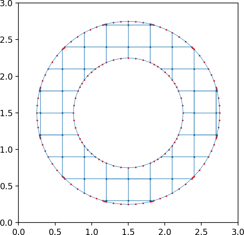
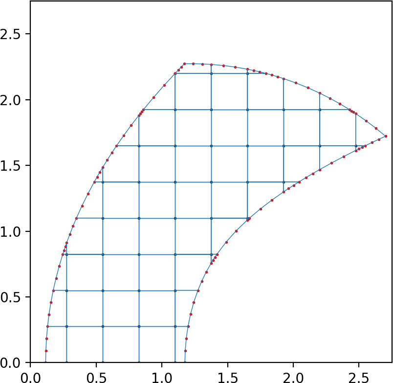
This is a short Python code that generates two dimensional high order embedded boundary grids. The code is fast, with most operations fully vectorized in Numpy. There are a number of domains already implemented from [1], that include an annulus domain as well as the domain used in Ringleb flow.
High order embedded boundary annulus (left) and Ringleb (right) domains. Each curved boundary segment has q+1 boundary points (red dots), where q = 3.
To install, navigate to the cloned github repository, and call
pip install -e .
The goal of this work is to provide an easy to install, high order cut cell grid generator for simple boundary geometries that have a functional representation. PyGrid assumes that each cut cell has only one or two, possibly curved, edges associated to the embedded boundary.
Zooms onto cut cells of the annulus and Ringleb meshes. Cut cells can have either one (left) or two curved edges (right). Cut cells with two curved edges can occur on sharp corners of the embedded boundary.
The code supports complex curved embedded boundaries (illustrated below), provided that it has a functional representation. We do not allow split or tunneled cells for ease of code development. This mesh generator does not handle mesh degeneracies, nor can it handle all types of cut cells, see the section entitled The sharp bits below for more information on the codes limitations.
Complex curved embedded boundaries are also supported. Here we embedded five `blobs' and request three interpolation points per cut cell edge ().
-
The user provides a function,
in_domain, that maps a spatial coordinate (x,y) to 1 if the point lies inside the domain or 0 if it does not. Using this function, the regular grid points that lie in and out of the domain are determined. For example, this is done in the figure below on the Ringleb domain. The regular grid points that lie in the domain are shown in orange, while the regular grid points that are outside the domain are shown in black. -
When a regular grid point that lies outside the domain is adjacent another that is inside the domain, this means that between these two points, the embedded boundary crosses a Cartesian grid line. Using the method of bisection, the precise point of intersection is computed. On the Ringleb domain below, these points are plotted in red. Right now, the code assumes that the boundary does not cross the grid line more than once.
-
After these intersection points are computed, the cut cells are assembled.
-
If the user requests curved edges, then additional vertices that are approximately uniformly spaced (in arclength) along the embedded boundary are computed. For circular embedded boundaries, we have explicit formulae to accomplish this. Again, this is done using the method of bisection.
-
The cut cells are then written to file in the
.plyformat. See here for more information http://paulbourke.net/dataformats/ply/.
Regular grid points that lie inside and outside the domain are respectively orange and black, computed in step 1. Irregular grid points on the embedded boundary are red, computed in step 2.
If curved boundaries are requested, the code computes interpolation points that are equispaced in arclength (for circular boundaries) and approximately equispaced in arclength using the method of bisection otherwise. The approach for non-circular boundaries relies on a one-dimensional parametrization of the boundary .
Say that a cut cell's curved edge is defined by the set of points
.
In order to find additional interpolation points along the boundary, define the function
for some on
. This function is zero when
maps to a point,
, that is exactly
units away from
.
Note that and
. Provided that
is monotonically increasing on
,
will only have a single root in
, which can be found using the method of bisection. Therefore, when the user requests
interpolation points along the boundary, the code finds the roots of
when
. These
additional boundary points, along with the edge endpoints
and
, form a set of
edge interpolation points.
Note that this is not a fully robust approach to determining interpolation points on the embedded boundary and is only appropriate when the boundary is sufficiently well-resolved.
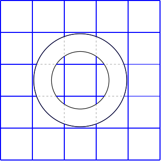
This code only handles cut cells on which the boundary enters and leaves on different faces. Additionally, it cannot deal with tunnelled and split cells. It may be added in the future, and of course in 3D for real geometries this would be necessary.
On the left, the annulus domain is removed from the background grid, creating split cut cells. On the right, the complement of the annulus is removed from the background grid, creating tunnelled cut cells.
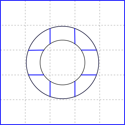
Additionally, the code does not robustly (or gracefully) handle mesh degeneracies. For example, if the embedded geometry lies directly on a Cartesian grid line cell, the code will produce erroneous output and may, or may not output an error.
A square domain (black lines) is removed from the background grid (blue lines), where the domain is perfectly aligned with the Cartesian grid lines.
We do not support the above scenarios for code simplicity, however, they must be addressed when moving to three dimensions and complex engineering geometries. This is the reason that the dimensions of some of the background grids in [1] are slighly perturbed from round numbers, as we aimed to avoid any of the above scenarios.
Of the many examples included here, the script in ./examples/8_argrun/driver.py accepts command line arguments, which are explained below:
-Nx number of cells on the grid in the x-direction
-Ny number of cells on the grid in the y-direction
-fbody the ID of the embedded boundary to be used.
0: quarter annulus, for the supersonic vortex problem,1: annulus for rotating pulse problem,2: Ringleb,3: random blobs.4: annulus for acoustics problem,5: circular obstacles,6: channel,7: double Mach.
-plot display the generated cut cell grid
-q add curved edges on the cut cells with q+1 interpolation points with the embedded boundary
For example, the Ringleb domain can be generated and plotted by calling
./examples/8_argrun/driver.py -Nx 10 -Ny 10 -fbody 2 -q 3 -plot
For help running the code, or any other questions, send me an email at
giuliani AT cims DOT nyu DOT edu
If you find this code useful in your work, you can cite it with
Giuliani, Andrew. "A two-dimensional stabilized discontinuous Galerkin method on curvilinear embedded boundary grids". https://arxiv.org/abs/2102.01857
[1] Giuliani, Andrew. "A two-dimensional stabilized discontinuous Galerkin method on curvilinear embedded boundary grids". https://arxiv.org/abs/2102.01857


