2018 Insight Data Engineering project
The project extracted and integrated cancer research data from GDC Data Portal of National Cancer Institute to patient-indexed tables in PostgreSQL on Amazon RDS via Spark, thus enabled cancer-wide, genome-wide queries on cancer data via SQL or other analytic tools.
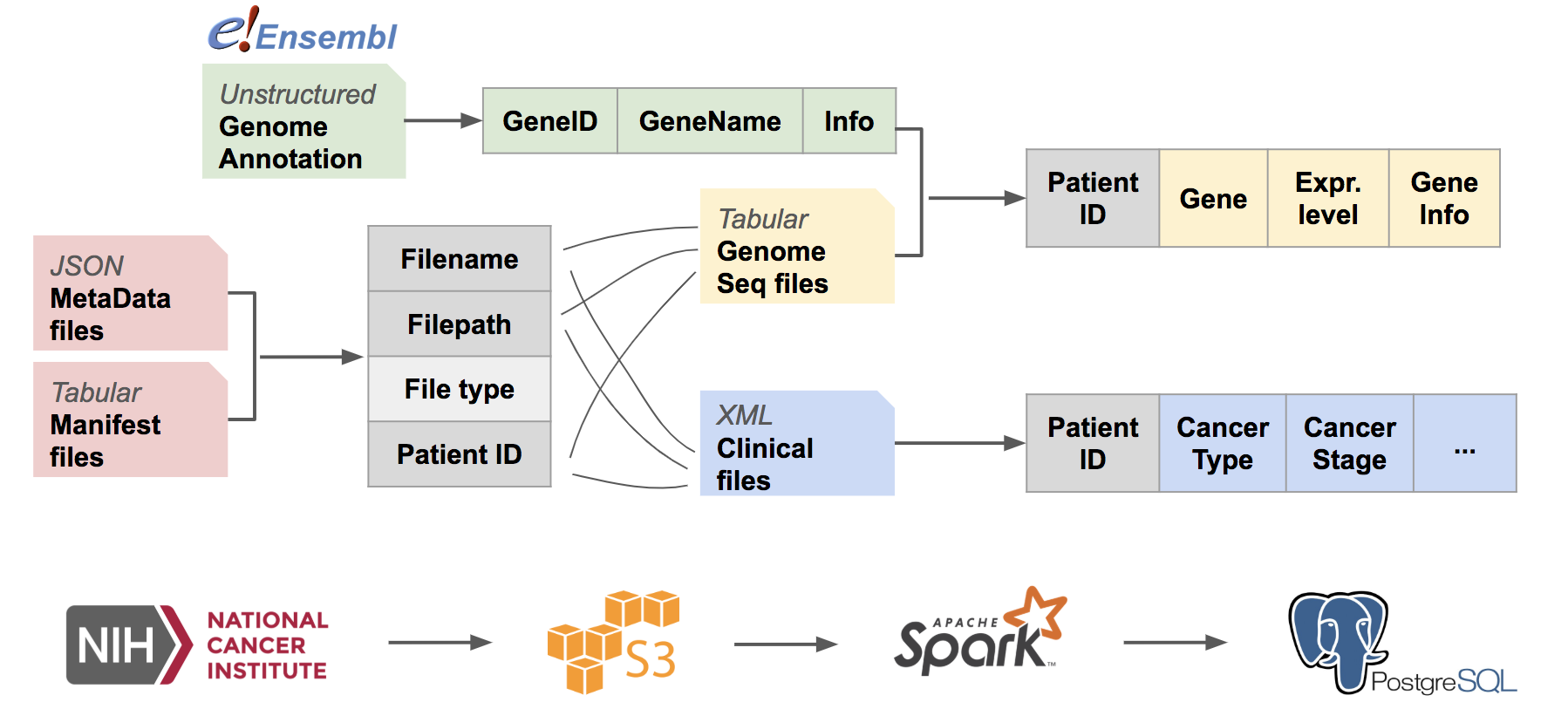
ETL pipeline is described below:
The pipeline can be divided into 2 stages:
- Generation of file look-up table
- Individual file parsing and information extraction.
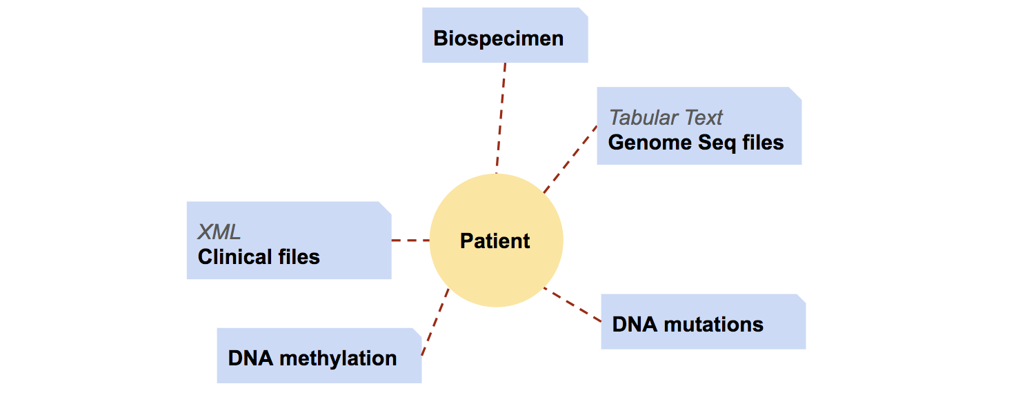
In data portal of National Cancer Institute, each patient may have multiple feature files, and each feature file contains one aspect of information from one individual patient. Moreover, it isn't possible to tell which patient one file belongs to from the files directly.
To index the files downloaded from NCI, I created a file look-up table in psql with two meta data files:
-
Manifest files: Tabular CSV files, from which I retrieved filename and where the files are stored after downloading.
-
MetaInfo files: Json files, from which I retrieved filename, file type, patient id, and project id (the project that collected the patient's information).
With PySpark, I joined the two tables on filenames, grouped the files by their types, and saved the information to tables in PostgreSQL database.
Due to time limit of the project, xml files and txt files were saved in separate tables for further information extraction.
All the other file types are saved in another table, for future use.
Schema of xml_list table:
| path | filename | data_format | project_id | case_id |
|---|---|---|---|---|
| text | text | text | text | text |
Meanwhile, with the patient id information extracted from meta info files, I created another table in psql, named patient_info. This table, with patient id
as primary key, in psql.
patient_info table will also save information about the project the patient enrolled in, and later the clinical information,
such as patient gender, disease type and disease stage, from clinical xml files.
Schema of patient_info table:
| case_id | project_id | disease_type | disease_stage | gender |
|---|---|---|---|---|
| text PRIMARY KEY UNIQUE | text | text | text | text |
As mentioned above, clinical reports are saved as xml format files. From these files, I extracted information of
patient gender, primary tumor site, and tumor stage (if applicable).
Because each xml file is only 100kb, and each file will update one row in table patient_info, I read in
xml file list from xml_list table in psql with Spark, and split the further tasks: file reading and info extraction, to
separate partitions. In each partition, I parsed the xml file with Python built-in xml reader.
Further, the extracte information was updated in batch (by partition) to patient_info table.
The optimization and design logic of xml file processor can be found in wikipage.
For normalization, RNA-seq data are stored in a separate table, gene_expr_table.
gene_expr_table is indexed with both patient id and gene id.
To start with, an empty table with headers: case_id(patient id), gene_id and gene_expr is created:
| case_id | gene_id | gene_expr |
|---|---|---|
| text | text | float |
Genome squencing results are saved in tabular txt files. For each partition of files, the txt files are
parsed and appended to gene_expr_table together with patient id.
After data is saved to database, the gene_expr_table is indexed with B-tree.
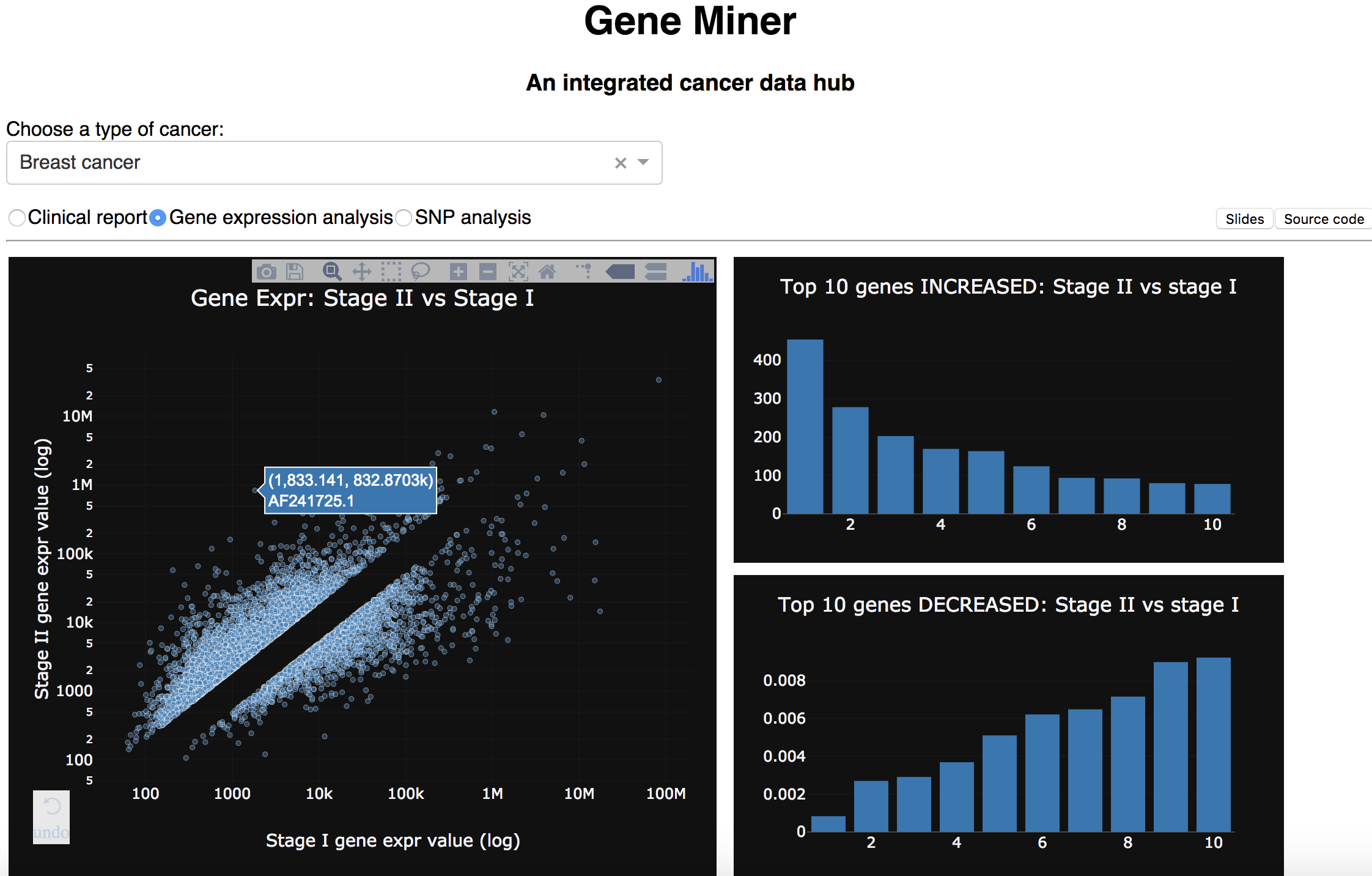
Top 10 genes changed between Stage II and Stage I of breast cancer
(See SQL code here.)
Based on disease_type and disease_stage columns patient_info table, patient_id associated with specific cancer type and
specific tumor stages are filtered out and grouped.
These patient_id are then used to filter out the genes associated with specific diseases and stages in gene_expr_table,
groupby gene_id.
After having the avg gene expression levels for each stage, the fold change between stages were calculated by dividing the values.
Finally, the (gene_id, fold_change) table is joined with reference genome table.
-
Reference genome table
hs_genomewas generated by Python via parsing annotated genome files from Ensembl. Information of genes from in total 24 chromosomes plus mitochondrial and non-chromosomal were extracted and saved to psql.hs_genometable has the schema:full_id id name chromosome strand pos_start pos_end info text text text text text integer integer text
After sorting by fold_change, the top10 table came with schema:
| gene_id | gene_name | fold_change | chromosome | info |
|---|---|---|---|---|
| text | text | float | text | text |
Which are visualized in bar chart and showed in demo .
The jobs were run on 4 m4.large EC2 instances.
The PostgreSQL database was created in Amazon RDS under the same VPC as EC2 instances.
The setup for instances, Spark, Jupyter notebook and postgresql can be found in
wikipage.
The Anaconda environment used to run the project can be found in environment.yml.
# Python versions
    python = 3.6.5
    pyspark = 2.2.0
# Python packages
    psycopg2 = 2.7.4 # To connect to PostgreSQL
    boto3 = 1.7.4  # To connect to S3
Tha packages above should be available on both mater and workers.
# Driver packages
# PosgreSQL
    postgresql-42.2.2.jar

# Redshift
# NOTE: This is the combination that won't cause any compatibility issue
    spark-redshift_2.11-3.0.0-preview1.jar
    RedshiftJDBC41-1.2.12.1017.jar
    spark-avro_2.11-4.0.0.jar
    minimal-json-0.9.5.jar
# Front end
    flask = 1.0.2
    dash = 0.21.0
    dash-core-components = 0.22.1
    dash-html-components = 0.10.1
    gunicorn = 19.8.1
    pandas = 0.22.0
-
Set the
PYTHONPATHbefore running:export PYTHONPATH=$PYTHONPATH:/home/ubuntu/GeneMiner:/home/ubuntu/GeneMiner/src -
Python drivers, jars and sub-modules required manual distribution are set in python script.
-
To generate reference genome:
GeneMiner/src $ python ref_genome/genome_parser.py -
To generate file look-up table:
GeneMiner/src $ python pipeline/metainfo_processor.py -
To process each types of files:
GeneMiner/src $ python pipeline/xml_processor.pyGeneMiner/src $ python pipeline/rnaseq_processor.py -
To run the front-end:
GeneMiner/flask-dash-app $ python run.pyGeneMiner/flask-dash-app $ gunicorn app:app -D(Run in background)
-
The demo is built by plotly/dash and made publicly available via flask, gunicorn and nginx.
For more information about setting up the front end, refer to wikipage.
When applicable, the demo is running at site: http://www.oxphos.online.
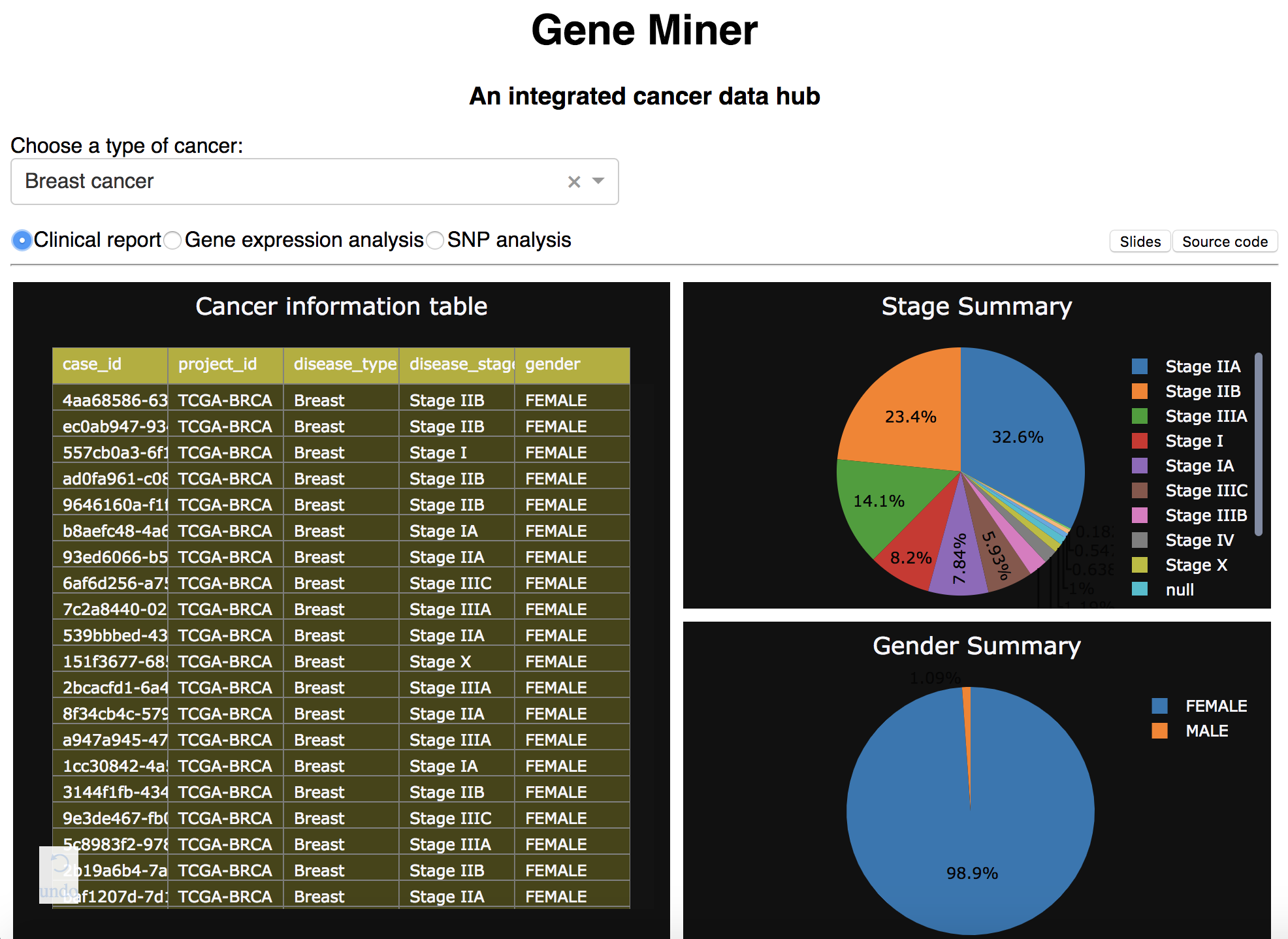
First, the website allows table display and summary view of patient clinical reports of different types and cancer (clinical reports):
Then, the website showcases one application of the data. For example, we can compare the gene expression change between Stage II and Stage I of breast cancer, and identify the top 10 genes that changed most between stages (gene expression analysis).


