


ABSTRACT
Using the Herschel Space Observatory we have observed a representative sample of 87 powerful 3CR sources at redshift  . The far-infrared (FIR, 70-500 μm) photometry is combined with mid-infrared (MIR) photometry from the Wide-Field Infrared Survey Explorer and cataloged data to analyze the complete spectral energy distributions (SEDs) of each object from optical to radio wavelength. To disentangle the contributions of different components, the SEDs are fitted with a set of templates to derive the luminosities of host galaxy starlight, dust torus emission powered by active galactic nuclei (AGNs), and cool dust heated by stars. The level of emission from relativistic jets is also estimated to isolate the thermal host galaxy contribution. The new data are in line with the orientation-based unification of high-excitation radio-loud AGN, in that the dust torus becomes optically thin longwards of
  . The low-excitation radio galaxies and the MIR-weak sources represent an MIR- and FIR-faint AGN population that is different from the high-excitation MIR-bright objects; it remains an open question whether they are at a later evolutionary state or an intrinsically different population. The derived luminosities for host starlight and dust heated by star formation are converted to stellar masses and star-formation rates (SFR). The host-normalized SFR of the bulk of the 3CR sources is low when compared to other galaxy populations at the same epoch. Estimates of the dust mass yield a 1–100 times lower dust/stellar mass ratio than for the Milky Way, which indicates that these 3CR hosts have very low levels of interstellar matter and explains the low level of star formation. Less than 10% of the 3CR sources show levels of star formation above those of the main sequence of star-forming galaxies.
Export citation and abstract BibTeX RIS
1. INTRODUCTION
In the current paradigm of active galactic nucleus (AGN) evolution, galaxy collisions and mergers lead to the genesis of powerful radio sources (Heckman et al. 1986). Based on far-infrared (FIR) studies with the Infrared Astronomical Satellite (IRAS) in the 1980s, the Palomar-Green (PG) quasars appeared to be preceded or accompanied by violent dust-enshrouded starburst activity (Sanders et al. 1988, 1989; Rowan-Robinson 1995). Refined Infrared Space Observatory (ISO) photometry in the 1990s indicated a potential evolution from FIR-bright to FIR-faint AGN states (see Haas et al. 2003).
Searching for the unbeamed counterparts of the quasar population in the medium-redshift ( ) sample from the Revised Third Cambridge Catalog of Radio Sources (3CR), Barthel (1989, 1994) proposed the orientation-based unification scheme of quasars and high-excitation radio galaxies (HERGs). Consensus is growing that this scheme is basically valid for sources with high radio power (
 ).
).
The sample is subdivided by the classification criteria based on radio and optical properties. In compact steep-spectrum (CSS) sources, the radio emission is restricted to regions of less than 20 kpc. Fanaroff–Riley Class I (FRI) sources show edge-dimmed radio lobes, while in FRII sources the lobes are brighter at the edge. The type-1 sources have optical bright continua and broad emission lines and are called Broad-Line Radio Galaxies (BLRG) at low luminosity. The high luminosity Flat-Spectrum-Quasars (FSQs) show flat radio spectra in  , in contrast to Steep-Spectrum-Quasars (SSQs) that have a dividing spectral index
  measured at a few GHz. Type-2 sources show only narrow emission lines and have weak optical continua, High-Excitation RGs (HERGs) have [O iii]/[O ii] > 1, and Low-Excitation RGs (LERGs) have [O iii]/[O ii] < 1 (
![${\lambda }_{[{\rm{O}}{\rm{II}}]}=3727\;\mathring{A}$](https://content.cld.iop.org/journals/1538-3881/151/5/120/revision1/aj523019ieqn7.gif) ,
, ![${\lambda }_{[{\rm{O}}{\rm{III}}]}=5007\;\mathring{A}$](https://content.cld.iop.org/journals/1538-3881/151/5/120/revision1/aj523019ieqn8.gif) ).
).
The 3CR radio sources can be subdivided into many different classes (e.g., quasars and radio galaxies), and demographic arguments have questioned whether every edge-brightened double-lobe FR II radio galaxy is a misaligned hidden quasar. At low redshift ( ) where the radio power of the 3CR sample reaches down to
  , narrow-line radio galaxies outnumber the quasars and BLRGs, mainly due to the contribution of low-excitation radio galaxies (LERGs; Laing et al. 1983; Singal 1993).
Based on mid-infrared (MIR) observations with VISIR, ISOCAM (Siebenmorgen et al. 2004; van der Wolk et al. 2010), and Spitzer (Ogle et al. 2006), the LERGs and a few HERGs are MIR-weak, indicating that they either do not possess high accretion power comparable to the MIR-strong HERGs and quasars/BLRGs or that they are more strongly extincted. FIR observations may be able to discriminate between the two scenarios, but in view of the expected faintness, such observations have not been performed so far. Only a few dozen bright HERGs and quasars/BLRGs have been detected in the FIR with ISO7 as compiled by Haas et al. (2004).
This work studies a sample of 87 sources from the 3CR catalog (Edge et al. 1959; Bennett 1962; Laing et al. 1983; Spinrad et al. 1985). With the Herschel Space Observatory (Pilbratt et al. 2010) we measured the FIR/submm spectral energy distributions (SEDs) of the 3CR sources in two complementary proposals: one at redshift  (PI: Barthel, Barthel et al. 2012; Podigachoski et al. 2015b, 2015a) and one at medium (
 ) and low (
 ) redshift (PI: Haas).
We here present sensitive Herschel Photoconducter Array Camera and Spectrometer (PACS)/Spectral and Photometric Imaging Receiver (SPIRE) 70–500 μm photometry of the representative 3CR sample at low and medium redshift. The FIR properties of this 3CR sample were already measured with the previous IR satellites (IRAS: Heckman et al. 1992, 1994; Hes et al. 1995; Hoekstra et al. 1997; ISO: Fanti et al. 2000; Polletta et al. 2000; van Bemmel et al. 2000; Meisenheimer et al. 2001; Andreani et al. 2002; Haas et al. 2004 and the Spitzer Space Telescope: Haas et al. 2005; Ogle et al. 2006; Cleary et al. 2007). The new FIR observations with Herschel benefit from the higher spatial resolution and sensitivity of the instruments.
We here analyze the full optical to radio SEDs, also combined with Wide-Field Infrared Survey Explorer (WISE) 3–22 μm photometry. The purpose is to explore dust emission in the FIR for the most powerful radio-loud AGN, provide constraints on the star-forming activity, and investigate the evolutionary status of their host galaxies.
We adopt a standard ΛCDM cosmology ( km s−1 Mpc−1,
  , and
, and  , Spergel et al. 2007).
2. SAMPLE
2.1. Medium-redshift Sample 

The sample properties for 3CR sources at medium redshifts, which were observed by Herschel in the two open time programs from the OT1_mhaas_2 and OT1_jstevens_1 proposals, are given in Table 1. From the 48 sources at  in the 3CR catalog, a representative subset of 39 was observed. The sources are selected to be brighter than 10 Jy at a frequency of 178 MHz (Laing et al. 1983). The sources that were not observed with Herschel do not bias the remaining subsample because their types are well represented. For the observed sources MIR photometry and/or spectroscopy from the Spitzer Space Telescope can be found in Ogle et al. (2006) and Cleary et al. (2007). Two FSQs (3C 345, 3C 454.3), one SSQ (3C 275.1), four HERGs (3C 34, 3C 217, 3C 247, 3C 277.2), and one LERG (3C 41) are in the 3CR catalog but not observed by Spitzer. Two HERGs, 3C 175.1 and 3C 220.3, were removed from the analysis. The former has insufficient ancillary data in the literature, and the latter acts as gravitational lens for a submillimeter galaxy at z = 2.2 (Haas et al. 2014).
Table 1.
3CR Sources  Observed with Herschel
| Name | R.A. [J2000] | Decl. [J2000] | Redshift |
 (Mpc) (Mpc) |
Type | Proposal-IDa | PACS-OBSID | SPIRE-OBSID |
|---|---|---|---|---|---|---|---|---|
| 3C006.1 | 00 16 31.1 | +79 16 50 | 0.8404 | 5193 | HERG | 1 | 1342262061/62 | ⋯ |
| 3C022.0 | 00 50 56.3 | +51 12 03 | 0.9360 | 5935 | BLRG | 2 | 1342237866/67 | ⋯ |
| 3C049.0 | 01 41 09.1 | +13 53 28 | 0.6207 | 3568 | HERGb | 1 | 1342261865/66 | ⋯ |
| 3C055.0 | 01 57 10.5 | +28 51 38 | 0.7348 | 4392 | HERG | 1 | 1342261794/95 | 1342261703 |
| 3C138.0 | 05 21 09.9 | +16 38 22 | 0.7590 | 4578 | QSRb | 1 | 1342267270/71 | 1342268340 |
| 3C147.0 | 05 42 36.1 | +49 51 07 | 0.5450 | 3048 | QSRb | 1 | 1342268972/73 | ⋯ |
| 3C172.0 | 07 02 08.3 | +25 13 53c | 0.5191 | 2876 | HERG | 1 | 1342268994/95 | ⋯ |
| 3C175.0 | 07 13 02.4 | +11 46 15 | 0.7700 | 4665 | QSR | 1 | 1342269004/05 | ⋯ |
| 3C175.1 | 07 14 04.7 | +14 36 22 | 0.9200 | 5820 | HERG | 2 | 1342242694/95 | 1342230780 |
| 3C184.0 | 07 39 24.2 | +70 23 11c | 0.9940 | 6406 | HERG | 2 | 1342243742/43 | 1342229126 |
| 3C196.0 | 08 13 36.0 | +48 13 03 | 0.8710 | 5436 | QSR | 1 | 1342254180/81 | ⋯ |
| 3C207.0 | 08 40 47.6 | +13 12 24 | 0.6806 | 4009 | QSR | 1 | 1342254575/76 | ⋯ |
| 3C216.0 | 09 09 33.5 | +42 53 46 | 0.6699 | 3929 | QSRb | 1 | 1342254561/62 | 1342255115 |
| 3C220.1 | 09 32 39.6 | +79 06 32 | 0.6100 | 3498 | HERG | 1 | 1342254194-96 | ⋯ |
| 3C220.3 | 09 39 23.8 | +83 15 26c | 0.6800 | 3997 | LENS | 1 | 1342221818/19 | 1342254521 |
| 3C226.0 | 09 44 16.5 | +09 46 17c | 0.8177 | 5030 | HERG | 1 | 1342255958/59 | 1342255165 |
| 3C228.0 | 09 50 10.8 | +14 20 01 | 0.5524 | 3106 | HERG | 1 | 1342255462-64 | ⋯ |
| 3C254.0 | 11 14 38.7 | +40 37 20 | 0.7366 | 4418 | QSR | 1 | 1342255900/01 | ⋯ |
| 3C263.0 | 11 39 57.0 | +65 47 49 | 0.6460 | 3755 | QSR | 1 | 1342255428-30 | ⋯ |
| 3C263.1 | 11 43 25.1 | +22 06 56 | 0.8240 | 5078 | HERG | 1 | 1342255685-87 | ⋯ |
| 3C265.0 | 11 45 29.0 | +31 33 47c | 0.8110 | 4978 | HERG | 1 | 1342255485/86 | ⋯ |
| 3C268.1 | 12 00 24.5 | +73 00 46c | 0.9700 | 6214 | HERG | 2 | 1342245706/07 | 1342229628 |
| ⋯ | ⋯ | ⋯ | ⋯ | ⋯ | ⋯ | 1342247316/17 | ⋯ | |
| 3C280.0 | 12 56 57.8 | +47 20 20c | 0.9960 | 6426 | HERG | 2 | 1342233434/35 | 1342232704 |
| 3C286.0 | 13 31 08.3 | +30 30 33 | 0.8499 | 5275 | QSRb | 1 | 1342259326/27 | 1342259451 |
| 3C289.0 | 13 45 26.4 | +49 46 33 | 0.9674 | 6196 | HERG | 2 | 1342233495/96 | 1342232711 |
| 3C292.0 | 13 50 41.9 | +64 29 36c | 0.7100 | 4218 | HERG | 1 | 1342257595-97 | ⋯ |
| 3C309.1 | 14 59 07.6 | +71 40 20 | 0.9050 | 5698 | QSRb | 1 | 1342259354-57 | ⋯ |
| 3C330.0 | 16 09 34.9 | +65 56 38c | 0.5500 | 3082 | HERG | 1 | 1342261369/70 | ⋯ |
| 3C334.0 | 16 20 21.8 | +17 36 24 | 0.5551 | 3118 | QSR | 1 | 1342261319/20 | 1342263861 |
| 3C336.0 | 16 24 39.1 | +23 45 12 | 0.9265 | 5868 | QSR | 1 | 1342261324-27 | ⋯ |
| 3C337.0 | 16 28 52.5 | +44 19 07c | 0.6350 | 3674 | HERG | 1 | 1342261350-53 | ⋯ |
| 3C340.0 | 16 29 36.6 | +23 20 13c | 0.7754 | 4702 | HERG | 1 | 1342261321-23 | ⋯ |
| 3C343.0 | 16 34 33.8 | +62 45 36 | 0.9880 | 6356 | HERGb,c | 2 | 1342234218/19 | ⋯ |
| 3C343.1 | 16 38 28.2 | +62 34 44 | 0.7500 | 4511 | HERGb | 1 | 1342261364-66 | ⋯ |
| 3C352.0 | 17 10 44.1 | +46 01 29 | 0.8067 | 4937 | HERG | 1 | 1342256219-21 | ⋯ |
| 3C380.0 | 18 29 31.8 | +48 44 46 | 0.6920 | 4081 | QSRb | 1 | 1342257947/48 | ⋯ |
| 3C427.1 | 21 04 06.8 | +76 33 11 | 0.5720 | 3230 | LERG | 1 | 1342261377/78 | ⋯ |
| 3C441.0 | 22 06 04.9 | +29 29 20 | 0.7080 | 4193 | HERG | 1 | 1342221833-36 | ⋯ |
| 3C455.0 | 22 55 03.9 | +13 13 34 | 0.5430 | 3026 | HERGb,c | 1 | 1342258014-17 | ⋯ |
Notes.
a1 = OT1_mhaas_2, 2 = OT1_jstevens_1. bCSS. cCoordinates/classifiaction revised.Download table as: ASCIITypeset image
Thus a sample of 37 representative sources was analyzed: seven FSQs (six of them CSS), seven SSQs (one BLRG), twenty-two HERGs (four CSS), and one LERG.
2.2. Low-redshift Sample

The 3CR sample properties at low redshifts are shown in Table 2. It contains 48 sources at  , of which 40 sources are included in the 3CR catalog (Laing et al. 1983). From the Spinrad et al. (1985) version of 3CR sources, which extends to lower declinations, 4 additional sources belong to this sample. Mainly taken from the OT1_mhaas_2 proposal, the whole Herschel Science Archive (HSA) was searched for 3C-sources and the complete Herschel-observed list was collected, which was also observed in the OT1_pogle01_1, OT1_rmushotz_1, OT1_lho_1 and OT1_dfarrah_1 proposals.
Table 2.
3CR Sources  Observed with Herschel
| Name | R.A. [J2000] | Decl. [J2000] | Redshift |
 (Mpc) (Mpc) |
Type | Proposal-IDa | PACS-OBSID | SPIRE-OBSID |
|---|---|---|---|---|---|---|---|---|
| 3C020.0 | 00 43 09.2 | +52 03 36b | 0.1740 | 804 | HERG | 1 | ⋯ | 1342265338 |
| 3C031.0 | 01 07 24.9 | +32 24 45 | 0.0170 | 66 | LERGc | 3 | 1342224218/19 | 1342236245 |
| 3C033.0 | 01 08 52.9 | +13 20 14b | 0.0597 | 252 | HERG | 1 | 1342261863/64 | ⋯ |
| 3C033.1 | 01 09 44.3 | +73 11 57b | 0.1810 | 842 | BLRG | 1 | 1342261944-46 | ⋯ |
| 3C035.0 | 01 12 02.3 | +49 28 36b | 0.0670 | 286 | HERG | 1 | 1342261413-16 | ⋯ |
| 3C047.0 | 01 36 24.4 | +20 57 28b | 0.4250 | 2252 | QSR | 1 | ⋯ | 1342261707 |
| 3C048.0 | 01 37 41.3 | +33 09 35 | 0.3670 | 1892 | QSRd | 1 | ⋯ | 1342261702 |
| 3C079.0 | 03 10 00.1 | +17 05 59b | 0.2559 | 1244 | HERG | 1 | 1342262229/30 | ⋯ |
| 3C098.0 | 03 58 54.4 | +10 26 03 | 0.0305 | 126 | HERG | 1 | 1342267198/99 | ⋯ |
| 3C109.0 | 04 13 40.4 | +11 12 15b | 0.3056 | 1529 | BLRG | 1 | 1342267272/73 | 1342266668 |
| 3C111.0 | 04 18 21.3 | +38 01 36 | 0.0485 | 205 | BLRG | 4 | 1342239439/40 | 1342229105 |
| 3C120.0 | 04 33 11.1 | +05 21 16 | 0.0330 | 138 | BLRG | 4 | 1342241955/56 | 1342239936 |
| 3C123.0 | 04 37 04.4 | +29 40 14 | 0.2177 | 1037 | LERG | 1 | 1342267256-59 | ⋯ |
| 3C153.0 | 06 09 32.5 | +48 04 15 | 0.2769 | 1367 | LERG | 1 | 1342267224-27 | ⋯ |
| 3C171.0 | 06 55 14.8 | +54 08 57b | 0.2384 | 1152 | HERG | 1 | 1342267228/29 | ⋯ |
| 3C173.1 | 07 09 18.2 | +74 49 32b | 0.2921 | 1453 | LERG | 1 | 1342265540/41 | ⋯ |
| 3C192.0 | 08 05 35.0 | +24 09 50 | 0.0597 | 260 | HERG | 1 | 1342254172/73 | ⋯ |
| 3C200.0 | 08 27 25.4 | +29 18 45 | 0.4580 | 2475 | LERG | 1 | 1342254174-77 | ⋯ |
| 3C219.0 | 09 21 08.6 | +45 38 57 | 0.1747 | 815 | BLRG | 1 | 1342254559/60 | ⋯ |
| 3C234.0 | 10 01 49.5 | +28 47 09 | 0.1849 | 870 | HERG | 1 | 1342255459 | 1342255182 |
| 3C236.0 | 10 06 01.8 | +34 54 10b | 0.1005 | 449 | LERG | 3 | 1342246697/98 | 1342246613 |
| ⋯ | ⋯ | ⋯ | ⋯ | ⋯ | 1 | 1342270912/13 | ⋯ | |
| 3C249.1 | 11 04 13.9 | +76 58 58b | 0.3115 | 1566 | QSR | 5 | 1342221763-66 | 1342229630 |
| 3C268.3 | 12 06 24.7 | +64 13 37 | 0.3717 | 1928 | BLRGd | 1 | 1342255424/25 | ⋯ |
| 3C273.0 | 12 29 06.7 | +02 03 09 | 0.1583 | 734 | QSR | 6 | ⋯ | 1342234882 |
| 3C274.1 | 12 35 26.7 | +21 20 35 | 0.4220 | 2246 | HERG | 1 | 1342258032-35 | ⋯ |
| 3C285.0 | 13 21 17.9 | +42 35 15 | 0.0794 | 349 | HERG | 1 | 1342258514/15 | 1342256880 |
| 3C300.0 | 14 22 59.8 | +19 35 37b | 0.2700 | 1331 | HERG | 1 | 1342262509-12 | ⋯ |
| 3C305.0 | 14 49 21.6 | +63 16 14 | 0.0416 | 177 | HERGc | 3 | 1342223959/60 | 1342234915 |
| 3C310.0 | 15 04 57.1 | +26 00 58b | 0.0538 | 233 | LERGc | 3 | 1342235116/17 | 1342234778 |
| 3C315.0 | 15 13 40.1 | +26 07 31 | 0.1083 | 484 | HERGc | 3 | 1342224636/37 | 1342234777 |
| 3C319.0 | 15 24 04.9 | +54 28 06b | 0.1920 | 903 | LERG | 1 | 1342231879-82 | ⋯ |
| 3C321.0 | 15 31 43.5 | +24 04 19 | 0.0961 | 426 | HERG | 1 | ⋯ | 1342261679 |
| 3C326.0 | 15 52 09.1 | +20 05 24b | 0.0895 | 395 | LERG | 3 | 1342248732/33 | 1342238327 |
| 3C341.0 | 16 28 04.0 | +27 41 39b | 0.4480 | 2406 | HERG | 1 | 1342261328/29 | ⋯ |
| 3C349.0 | 16 59 28.9 | +47 02 55b | 0.2050 | 970 | HERG | 1 | 1342261354/55 | ⋯ |
| 3C351.0 | 17 04 41.4 | +60 44 30b | 0.3719 | 1927 | QSR | 5 | 1342232428-31 | 1342229147 |
| 3C381.0 | 18 33 46.3 | +47 27 03 | 0.1605 | 737 | BLRG | 1 | 1342261360/61 | ⋯ |
| 3C382.0 | 18 35 03.4 | +32 41 47 | 0.0579 | 246 | BLRG | 1 | 1342256206/07 | ⋯ |
| 3C386.0 | 18 38 26.2 | +17 11 50b | 0.0169 | 68 | LERGc | 3 | 1342231672/73 | 1342239789 |
| 3C388.0 | 18 44 02.4 | +45 33 30 | 0.0917 | 401 | LERG | 1 | 1342261356-59 | ⋯ |
| 3C390.3 | 18 42 08.9 | +79 46 17b | 0.0561 | 239 | BLRG | 1 | 1342221871/72 | ⋯ |
| 3C401.0 | 19 40 25.0 | +60 41 36b | 0.2011 | 947 | LERG | 1 | 1342256194-97 | ⋯ |
| 3C424.0 | 20 48 12.0 | +07 01 17 | 0.1270 | 567 | LERG | 3 | 1342233349/50 | 1342244149 |
| 3C433.0 | 21 23 44.5 | +25 04 28b | 0.1016 | 445 | HERGc | 1 | 1342219391/92 | ⋯ |
| ⋯ | ⋯ | ⋯ | ⋯ | ⋯ | 3 | 1342232731/32 | 1342234675 | |
| 3C436.0 | 21 44 11.7 | +28 10 19 | 0.2145 | 1016 | HERG | 3 | 1342235316/17 | 1342234676 |
| ⋯ | ⋯ | ⋯ | ⋯ | ⋯ | 1 | 1342257734-37 | ⋯ | |
| 3C438.0 | 21 55 52.3 | +38 00 28b | 0.2900 | 1435 | LERG | 1 | 1342259246-49 | ⋯ |
| 3C452.0 | 22 45 48.8 | +39 41 16 | 0.0811 | 349 | HERG | 1 | 1342259368/69 | ⋯ |
| 3C459.0 | 23 16 35.2 | +04 05 18 | 0.2201 | 1045 | BLRG | 3 | 1342237979/80 | 1342234756 |
Notes.
a1 = OT1_mhaas_2, 2 = OT1_jstevens_1, 3 = OT1_pogle01_1, 4 = OT1_rmushotz_1, 5 = OT1_lho_1, 6 = OT1_dfarrah_1. bcoordinates revised. cFR I. dCSS.Download table as: ASCIITypeset image
Spitzer MIR data are available for all sources. Twenty-three sources were observed in the flux limited sample of Ogle et al. (2006) with  . Four remaining sources from the Ogle sample were planned but not observed with Herschel. The rest of the sources were selected from samples already seen with Spitzer by Haas et al. (2005; also observed by the ISO satellite), Cleary et al. (2007), and Hardcastle et al. (2009; X-ray selection).
For the analysis the sample is subdivided into four FSQs (thereof three BLRGs), ten SSQs (thereof six BLRGs), nineteen HERGs, and fifteen LERGs. All but six sources (three HERGs and three LERGs) in this sample are morphologically classified as FR II sources (Fanaroff & Riley 1974).
3. DATA
For some objects of the medium-redshift sample a revision of the coordinates given in NED was necessary. We checked the positions given by Laing et al. (1983) and inspected WISE images. Positions from high resolution radio maps (Mullin et al. 2006; Haas et al. 2014) or positions seen with Chandra at 2–8 keV were taken whenever available. For the low-redshift sample, the coordinates were revised to match Willot's positions.8 Core positions from high resolution radio maps from VLA observation by Gilbert et al. (2004) were taken whenever available. The revised coordinates are indicated by footnotes in Tables 1 and 2. In addition, the classifications for 3C 343 and 3C 455 from NED were altered from QSR to HERG based on classification given by Véron-Cetty & Véron (2010).
3.1. Herschel PACS and SPIRE
The data were downloaded from the HSA within the framework of the Herschel Interactive Processing Environment (HIPE version 11.1.0, Ott 2010). For source extraction the tool SourceExtractor from Bertin & Arnouts (1996) was used and additional routines were developed in the Interactive Data Language (IDL) using the IDL Astronomy Library (Landsman 1993).
3.1.1. Observations
For the PACS (Poglitsch et al. 2010) the Scan-Map observational mode was chosen to observe the sources' photometrically at  (blue/green/red). In a single-scan, two filters (blue-red or green-red) were observed simultaneously. Often a cross-scan was done, which was two consecutive single-scans with different scan directions. The whole spectral range of PACS is covered by the combination of first scan in blue-red and the second in green-red; a double scan in the red filter was combined afterward to reach a higher sensitivity. For some sources, deeper imaging was achieved by the combination of multiple cross-scans.
SPIRE (Griffin et al. 2010) observes three bands at  (short/mid/long) at once. The Small-Scan-Map observational mode was chosen. For the medium-redshift sample the OBSIDs for the 98 PACS scans and 12 SPIRE scan-maps are shown in Table 1. The low-redshift sample was observed in 118 PACS scans and 23 SPIRE maps; OBSIDs are given in Table 2.
3.1.2. PACS-Reduction
The reduction of the PACS scan-maps was done in two steps, as bright sources have to be masked during the high-pass filtering (see Popesso et al. 2012). In the first step, a preliminary image is generated, which is then used to determine the positions for masking with SourceExtractor (only detections with nine pixels above a 3σ threshold are masked).
To minimize correlated noise and get a good signal-to-noise ratio, a pixel fraction of 0.6 and pixel sizes of 1 1 , 14, and 21 for the 70 μm, 100 μm, and 160 μm band was chosen, respectively. Additionally, the high-pass filter radius was set to 10, 15, and 20 readouts. Multiple scans were then combined with the mosaic task in HIPE.
The aperture corrected flux was determined for the pointlike sources in the frame. The target source was assumed to be that closest to and within  of the known source position (as listed in Tables 1 and 2). Images of size
  are shown in Appendix
We derived the photometric uncertainty as follows: Every frame comes with a coverage map that was used to generate 500 random positions on the map, where the coverage is greater than 75% of its maximum. At these positions, the HIPE routine annularSkyAperturePhotometry was used to perform aperture photometry with the background calculated in an annulus. Values for aperture and annulus radii (recommended for fluxes  mJy) given in Table 3 follow the Herschel Webinar for "PACS Point Source Photometry" by Paladini.9
The Gaussian dispersion of the 500 aperture corrected fluxes was adopted as the
mJy) given in Table 3 follow the Herschel Webinar for "PACS Point Source Photometry" by Paladini.9
The Gaussian dispersion of the 500 aperture corrected fluxes was adopted as the  uncertainty for each map (see also Leipski et al. 2013), and is listed in Tables 4 and 5. Where no sources could be detected, a 3σ upper limit is given.
Table 3. PACS Aperture and Annulus Radii
| 70 μm | 100 μm | 160 μm | |
|---|---|---|---|
| Aperture radius (") | 5.5 | 5.6 | 10.5 |
| Annulus inner radius (") | 20 | 20 | 24 |
| Annulus outer radius (") | 25 | 25 | 28 |
| Aperture correction | 0.61 | 0.57 | 0.63 |
Download table as: ASCIITypeset image
Table 4.
3CR Sources  PACS and SPIRE Flux Densities
| Name | Figure | F70 (mJy) | F100 (mJy) | F160 (mJy) | F250 (mJy) | F350 (mJy) | F500 (mJy) |
|---|---|---|---|---|---|---|---|
| 3C006.1 | Figure 4 | <14 | <15 | <30 | ⋯ | ⋯ | ⋯ |
| 3C022.0 | Figure 2 | 28(3) | ⋯ | <36 | ⋯ | ⋯ | ⋯ |
| 3C049.0 | Figure 3 | 16(4) | 25(5) | 27(7) | ⋯ | ⋯ | ⋯ |
| 3C055.0 | Figure 3 | 90(4) | 126(4) | 123(8) | 85(9) | 42(9) | <42 |
| 3C138.0 | Figure 1 | 47(4) | 49(5) | 58(10) | 64(11) | 70(15) | 103(14) |
| 3C147.0 | Figure 1 | 59(5) | 71(5) | 72(10) | ⋯ | ⋯ | ⋯ |
| 3C172.0 | Figure 5 | <9 | <14 | <28 | ⋯ | ⋯ | ⋯ |
| 3C175.0 | Figure 2 | 26(3) | 24(4) | <45 | ⋯ | ⋯ | ⋯ |
| 3C175.1 | Figure 7 | <8 | ⋯ | <22 | <62 | <50 | <38 |
| 3C184.0 | Figure 3 | 12(2) | ⋯ | <24 | <31 | <22 | <23 |
| 3C196.0 | Figure 2 | 24(3) | 18(4) | <34 | ⋯ | ⋯ | ⋯ |
| 3C207.0 | Figure 1 | 16(4) | 21(5) | 32(8) | ⋯ | ⋯ | ⋯ |
| 3C216.0 | Figure 1 | 79(3) | 102(5) | 143(9) | 204(8) | 229(14) | 266(22) |
| 3C220.1 | Figure 5 | <8 | <12 | <18 | ⋯ | ⋯ | ⋯ |
| 3C220.3 | Figure 7 | 26(3) | 99(4) | 259(11) | 452(9) | 412(8) | 259(7) |
| 3C226.0 | Figure 3 | 44(3) | 36(5) | <19 | <31 | <42 | <42 |
| 3C228.0 | Figure 5 | <8 | <15 | <23 | ⋯ | ⋯ | ⋯ |
| 3C254.0 | Figure 2 | 14(4) | <15 | <27 | ⋯ | ⋯ | ⋯ |
| 3C263.0 | Figure 2 | 56(4) | 43(4) | 27(8) | ⋯ | ⋯ | ⋯ |
| 3C263.1 | Figure 4 | <8 | <12 | <21 | ⋯ | ⋯ | ⋯ |
| 3C265.0 | Figure 3 | 40(4) | 47(6) | <41 | ⋯ | ⋯ | ⋯ |
| 3C268.1 | Figure 5 | <8 | ⋯ | <20 | <38 | <45 | <23 |
| 3C280.0 | Figure 3 | 24(3) | ⋯ | <31 | <38 | <32 | <40 |
| 3C286.0 | Figure 1 | 36(4) | 41(4) | 59(7) | 76(11) | 84(13) | 112(15) |
| 3C289.0 | Figure 4 | 10(3) | ⋯ | <21 | <32 | <33 | <35 |
| 3C292.0 | Figure 5 | <7 | <11 | <18 | ⋯ | ⋯ | ⋯ |
| 3C309.1 | Figure 1 | 43(3) | 35(4) | 39(9) | ⋯ | ⋯ | ⋯ |
| 3C330.0 | Figure 4 | <11 | <20 | <27 | ⋯ | ⋯ | ⋯ |
| 3C334.0 | Figure 2 | 69(3) | 71(4) | 51(8) | <40 | <33 | <67 |
| 3C336.0 | Figure 2 | <8 | <9 | <23 | ⋯ | ⋯ | ⋯ |
| 3C337.0 | Figure 5 | <6 | <9 | <13 | ⋯ | ⋯ | ⋯ |
| 3C340.0 | Figure 4 | <7 | <13 | <24 | ⋯ | ⋯ | ⋯ |
| 3C343.0 | Figure 3 | 58(2) | ⋯ | 73(11) | ⋯ | ⋯ | ⋯ |
| 3C343.1 | Figure 4 | 11(3) | <17 | <21 | ⋯ | ⋯ | ⋯ |
| 3C352.0 | Figure 5 | <7 | <12 | 19(4) | ⋯ | ⋯ | ⋯ |
| 3C380.0 | Figure 1 | 69(4) | 94(5) | 149(9) | ⋯ | ⋯ | ⋯ |
| 3C427.1 | Figure 6 | ⋯ | <6 | <18 | ⋯ | ⋯ | ⋯ |
| 3C441.0 | Figure 4 | 8(3) | <11 | <26 | ⋯ | ⋯ | ⋯ |
| 3C455.0 | Figure 4 | <6 | <8 | <18 | ⋯ | ⋯ | ⋯ |
Note. 1σ uncertainties are given in brackets; upper limits are 3σ.
Download table as: ASCIITypeset image
3.1.3. SPIRE-Reduction
For the photometry of the SPIRE observations, we followed the steps of the "Recipe for SPIRE Photometry."10
The recommended algorithm for point source photometry is the timeline-fitter, sourceExtractorTimeline in HIPE. To determine the positions of sources in the SPIRE maps, we used the level2 products of the observations in the HSA. A source list was generated within HIPE by sourceExtractorSussextractor. The coordinates of these sources were then used to perform the fitting in the timeline data on the level1 products in the HSA. The nearest source within  to the coordinates given in Tables 1 and 2 was identified as the 3CR target.
As for the uncertainty determination for the PACS observations, we used 500 randomly generated positions on the SPIRE maps, centered within 23 pixels of the center ( /
/ /
/ for
for  /
/ /
/ ). At these positions, the photometry was carried out in the same manner as for the sources. The dispersion of the distribution gave the 1σ uncertainty or 3σ upper limits, which are given in Tables 4 and 5. Images of size
  are shown in Appendix
Table 5.
3CR Sources  PACS and SPIRE Flux Densities
| Name | Figure | F70 (mJy) | F100 (mJy) | F160 (mJy) | F250 (mJy) | F350 (mJy) | F500 (mJy) |
|---|---|---|---|---|---|---|---|
| 3C020.0 | Figure 11 | ⋯ | ⋯ | ⋯ | 58(19) | 50(16) | <50 |
| 3C031.0 | Figure 15 | ⋯ | 867(3) | 1347(11) | 955(16) | 408(20) | 169(20) |
| 3C033.0 | Figure 11 | 161(4) | 194(4) | 179(8) | ⋯ | ⋯ | ⋯ |
| 3C033.1 | Figure 10 | 38(4) | 31(3) | <39 | ⋯ | ⋯ | ⋯ |
| 3C035.0 | Figure 13 | <6 | 16(3) | <23 | ⋯ | ⋯ | ⋯ |
| 3C047.0 | Figure 9 | ⋯ | ⋯ | ⋯ | <41 | <40 | <23 |
| 3C048.0 | Figure 9 | ⋯ | ⋯ | ⋯ | 311(10) | 137(13) | 62(10) |
| 3C079.0 | Figure 11 | 65(4) | 49(5) | 37(10) | ⋯ | ⋯ | ⋯ |
| 3C098.0 | Figure 12 | 41(5) | 49(4) | <37 | ⋯ | ⋯ | ⋯ |
| 3C109.0 | Figure 10 | 158(4) | 106(4) | 62(9) | <37 | <46 | <46 |
| 3C111.0 | Figure 8 | 242(6) | ⋯ | 461(24) | 577(27) | 741(26) | 876(31) |
| 3C120.0 | Figure 8 | 783(8) | ⋯ | 1145(20) | 634(9) | 465(13) | 439(16) |
| 3C123.0 | Figure 14 | 22(2) | 10(3) | <32 | ⋯ | ⋯ | ⋯ |
| 3C153.0 | Figure 14 | <8 | <10 | <20 | ⋯ | ⋯ | ⋯ |
| 3C171.0 | Figure 11 | 13(4) | <15 | <34 | ⋯ | ⋯ | ⋯ |
| 3C173.1 | Figure 14 | <10 | 13(4) | <30 | ⋯ | ⋯ | ⋯ |
| 3C192.0 | Figure 13 | 28(4) | 33(4) | <24 | ⋯ | ⋯ | ⋯ |
| 3C200.0 | Figure 14 | <7 | 12(3) | <18 | ⋯ | ⋯ | ⋯ |
| 3C219.0 | Figure 10 | <11 | <12 | <29 | ⋯ | ⋯ | ⋯ |
| 3C234.0 | Figure 11 | ⋯ | 87(4) | 46(13) | <40 | <47 | <38 |
| 3C236.0 | Figure 15 | 55(5) | 90(2) | 120(9) | 92(13) | 81(15) | 78(14) |
| 3C249.1 | Figure 9 | 64(3) | 62(3) | 45(6) | <39 | <46 | <31 |
| 3C268.3 | Figure 10 | 22(3) | 32(4) | <26 | ⋯ | ⋯ | ⋯ |
| 3C273.0 | Figure 8 | ⋯ | ⋯ | ⋯ | 475(16) | 683(11) | 1062(20) |
| 3C274.1 | Figure 13 | <6 | <10 | <19 | ⋯ | ⋯ | ⋯ |
| 3C285.0 | Figure 12 | 222(4) | 292(5) | 307(11) | 180(20) | 74(13) | <44 |
| 3C300.0 | Figure 13 | <6 | <8 | <19 | ⋯ | ⋯ | ⋯ |
| 3C305.0 | Figure 12 | ⋯ | 381(4) | 502(9) | 254(22) | 118(17) | <64 |
| 3C310.0 | Figure 15 | ⋯ | 23(1) | 38(3) | <30 | <43 | <41 |
| 3C315.0 | Figure 13 | ⋯ | 31(3) | 36(9) | <24 | <27 | <27 |
| 3C319.0 | Figure 14 | <7 | <11 | 31(8) | ⋯ | ⋯ | ⋯ |
| 3C321.0 | Figure 11 | ⋯ | ⋯ | ⋯ | 287(16) | 108(13) | <40 |
| 3C326.0 | Figure 15 | 6(2) | 15(1) | 19(4) | <30 | <20 | <23 |
| 3C341.0 | Figure 11 | 28(3) | <11 | <23 | ⋯ | ⋯ | ⋯ |
| 3C349.0 | Figure 12 | <11 | <12 | <23 | ⋯ | ⋯ | ⋯ |
| 3C351.0 | Figure 9 | 172(3) | 156(4) | 89(10) | <60 | <81 | <34 |
| 3C381.0 | Figure 10 | 35(4) | 34(5) | 39(10) | ⋯ | ⋯ | ⋯ |
| 3C382.0 | Figure 8 | 76(4) | 96(4) | 97(11) | ⋯ | ⋯ | ⋯ |
| 3C386.0 | Figure 15 | ⋯ | 66(3) | 81(9) | <90 | <43 | <43 |
| 3C388.0 | Figure 15 | <7 | <9 | <16 | ⋯ | ⋯ | ⋯ |
| 3C390.3 | Figure 10 | 157(4) | 110(4) | 51(8) | ⋯ | ⋯ | ⋯ |
| 3C401.0 | Figure 14 | <8 | <9 | <18 | ⋯ | ⋯ | ⋯ |
| 3C424.0 | Figure 14 | ⋯ | 7(1) | <13 | <22 | <39 | <28 |
| 3C433.0 | Figure 11 | 294(4) | 288(2) | 226(6) | 120(22) | <51 | <46 |
| 3C436.0 | Figure 13 | 16(3) | 30(2) | 37(5) | <51 | <30 | <40 |
| 3C438.0 | Figure 14 | <7 | <11 | <42 | ⋯ | ⋯ | ⋯ |
| 3C452.0 | Figure 12 | 38(4) | 36(5) | 27(8) | ⋯ | ⋯ | ⋯ |
| 3C459.0 | Figure 10 | ⋯ | 584(4) | 549(11) | 284(15) | 115(11) | 54(16) |
Note. 1σ-errors are given in brackets; upper limits are 3σ.
Download table as: ASCIITypeset image
Table 6.
Median Spectral Templates for Different Galaxy Types Separated for Low- (z < 0.5) and Medium-redshift (0.5  1)
1)
| HERG-low-z | HERG-med-z | LERG | BLRG | FSQ-low-z | FSQ-med-z | SSQ-low-z | SSQ-med-z | |
|---|---|---|---|---|---|---|---|---|

|

|

|

|

|

|

|

|

|
| (μm) |

|

|

|

|

|

|

|

|
| −0.4 | 10.4 ± 0.7 | 10.7 ± 0.4 | ⋯ | ⋯ | ⋯ | 11.8 ± 0.3 | ⋯ | 12.0 ± 0.6 |
| −0.3 | 10.7 ± 0.7 | 11.0 ± 0.3 | 10.6 ± 1.0 | 10.7 ± 0.5 | 11.0 ± 0.4 | 11.8 ± 0.2 | 11.6 ± 1.0 | 12.0 ± 0.6 |
| −0.2 | 11.0 ± 0.7 | 11.1 ± 0.3 | 10.8 ± 0.9 | 10.9 ± 0.5 | 10.9 ± 0.3 | 11.8 ± 0.2 | 11.6 ± 1.0 | 12.0 ± 0.6 |
| −0.1 | 10.9 ± 0.7 | 11.1 ± 0.3 | 11.0 ± 0.9 | 11.0 ± 0.4 | 10.9 ± 0.3 | 11.8 ± 0.2 | 11.6 ± 1.1 | 12.0 ± 0.4 |
| −0.0 | 11.0 ± 0.6 | 11.1 ± 0.2 | 11.0 ± 0.9 | 11.0 ± 0.4 | 10.9 ± 0.3 | 11.8 ± 0.2 | 11.6 ± 1.2 | 12.0 ± 0.4 |
| 0.1 | 11.1 ± 0.5 | 11.1 ± 0.2 | 11.2 ± 0.9 | 11.0 ± 0.3 | 10.8 ± 0.4 | 11.8 ± 0.2 | 11.7 ± 1.2 | 12.0 ± 0.4 |
| 0.2 | 11.0 ± 0.5 | 11.1 ± 0.2 | 11.1 ± 0.9 | 11.1 ± 0.3 | 10.9 ± 0.5 | 11.8 ± 0.2 | 11.7 ± 1.2 | 12.0 ± 0.4 |
| 0.3 | 10.9 ± 0.5 | 11.1 ± 0.2 | 11.1 ± 1.0 | 11.1 ± 0.3 | 11.0 ± 0.4 | 11.8 ± 0.2 | 11.7 ± 1.0 | 12.0 ± 0.4 |
| 0.4 | 10.9 ± 0.5 | 11.2 ± 0.2 | 10.5 ± 1.2 | 11.1 ± 0.3 | 11.0 ± 0.5 | 11.8 ± 0.2 | 11.7 ± 1.0 | 12.0 ± 0.3 |
| 0.5 | 10.7 ± 0.5 | 11.3 ± 0.3 | 10.3 ± 1.3 | 11.1 ± 0.4 | 11.0 ± 0.4 | 11.9 ± 0.2 | 11.7 ± 1.0 | 12.2 ± 0.3 |
| 0.6 | 10.6 ± 0.5 | 11.4 ± 0.3 | 9.9 ± 1.3 | 11.1 ± 0.4 | 10.9 ± 0.4 | 11.9 ± 0.2 | 11.7 ± 0.2 | 12.0 ± 0.2 |
| 0.7 | 10.6 ± 0.5 | 11.3 ± 0.3 | 9.5 ± 0.9 | 11.0 ± 0.5 | 10.9 ± 0.4 | 11.9 ± 0.2 | 11.8 ± 0.2 | 12.2 ± 0.3 |
| 0.8 | 10.7 ± 0.6 | 11.5 ± 0.3 | 9.6 ± 0.9 | 11.3 ± 0.5 | 11.0 ± 0.4 | 12.0 ± 0.2 | 11.9 ± 0.2 | 12.1 ± 0.3 |
| 0.9 | 10.7 ± 0.7 | 11.4 ± 0.3 | 9.4 ± 0.8 | 11.0 ± 0.5 | 10.9 ± 0.4 | 12.0 ± 0.2 | 11.9 ± 1.6 | 12.0 ± 0.3 |
| 1.0 | 10.8 ± 0.7 | 11.3 ± 0.3 | 9.4 ± 0.7 | 11.3 ± 0.5 | 10.9 ± 0.4 | 12.0 ± 0.2 | 12.0 ± 1.5 | 12.1 ± 0.3 |
| 1.1 | 10.8 ± 0.7 | 11.3 ± 0.3 | 9.6 ± 0.7 | 11.5 ± 0.5 | 10.8 ± 0.5 | 12.1 ± 0.2 | 11.7 ± 0.2 | 12.1 ± 0.4 |
| 1.2 | 10.9 ± 0.7 | 11.4 ± 0.4 | 9.8 ± 0.6 | 11.5 ± 0.4 | 10.7 ± 0.5 | 12.1 ± 0.2 | 12.1 ± 0.2 | 12.2 ± 0.4 |
| 1.3 | 10.9 ± 0.7 | 11.4 ± 0.3 | 9.8 ± 0.5 | 11.5 ± 0.5 | 10.7 ± 0.5 | 12.0 ± 0.2 | 12.1 ± 0.3 | 12.4 ± 0.3 |
| 1.4 | 10.8 ± 0.7 | 11.3 ± 0.5 | 9.5 ± 0.5 | 11.4 ± 0.5 | 10.6 ± 0.6 | 12.0 ± 0.2 | 12.2 ± 0.4 | 12.5 ± 0.5 |
| 1.5 | 10.8 ± 0.7 | 11.3 ± 0.5 | 10.6 ± 0.8 | 11.3 ± 0.5 | 10.5 ± 0.7 | 11.9 ± 0.2 | 12.1 ± 0.4 | 12.5 ± 0.5 |
| 1.6 | 10.8 ± 0.7 | 11.3 ± 0.5 | 10.7 ± 0.9 | 11.3 ± 0.5 | 10.4 ± 0.8 | 11.9 ± 0.3 | 12.1 ± 0.4 | 12.2 ± 0.7 |
| 1.7 | 10.8 ± 0.7 | 11.2 ± 0.6 | 10.6 ± 0.9 | 11.3 ± 0.5 | 10.3 ± 0.8 | 11.8 ± 0.3 | 11.9 ± 0.6 | 11.6 ± 0.8 |
| 1.8 | 10.5 ± 0.7 | 11.0 ± 0.7 | 10.4 ± 0.9 | 11.2 ± 0.7 | 10.2 ± 0.8 | 11.8 ± 0.3 | 11.8 ± 0.9 | 11.4 ± 0.8 |
| 1.9 | 10.3 ± 0.8 | 11.0 ± 0.7 | 10.0 ± 0.9 | 11.0 ± 0.8 | 10.3 ± 0.8 | 11.7 ± 0.3 | 11.7 ± 1.0 | 11.3 ± 0.8 |
| 2.0 | 10.2 ± 0.9 | 10.9 ± 0.7 | 9.8 ± 0.9 | 10.7 ± 0.9 | 10.3 ± 0.8 | 11.7 ± 0.3 | 11.6 ± 1.0 | 10.9 ± 0.8 |
| 2.1 | 10.1 ± 1.0 | 10.8 ± 0.6 | 9.7 ± 0.9 | 10.5 ± 0.9 | 10.2 ± 0.7 | 11.6 ± 0.3 | 11.3 ± 1.0 | 10.9 ± 0.8 |
| 2.2 | 9.9 ± 1.0 | 10.8 ± 0.6 | 9.5 ± 1.0 | 10.1 ± 0.8 | 10.2 ± 0.7 | 11.6 ± 0.3 | 11.1 ± 1.0 | 10.9 ± 0.8 |
| 2.3 | 9.7 ± 1.0 | 10.8 ± 0.6 | 9.5 ± 0.9 | 9.9 ± 0.8 | 10.2 ± 0.7 | 11.6 ± 0.3 | 11.0 ± 1.0 | 10.9 ± 0.8 |
| 2.4 | 9.6 ± 0.9 | 10.8 ± 0.6 | 9.3 ± 0.9 | 9.8 ± 0.8 | 10.2 ± 0.7 | 11.6 ± 0.3 | 10.9 ± 1.0 | 10.9 ± 0.8 |
| 2.5 | 9.5 ± 0.9 | 10.8 ± 0.6 | 9.2 ± 0.9 | 9.8 ± 0.8 | 10.2 ± 0.6 | 11.6 ± 0.3 | 10.7 ± 1.0 | 10.9 ± 0.8 |
| 3.0 | 9.4 ± 0.9 | 10.6 ± 0.6 | 9.2 ± 0.9 | 9.8 ± 0.8 | 10.1 ± 0.6 | 11.6 ± 0.3 | 10.3 ± 1.0 | 10.9 ± 0.8 |
| 3.4 | 9.4 ± 0.9 | 10.6 ± 0.6 | 9.2 ± 0.9 | 9.8 ± 0.8 | 10.0 ± 0.5 | 11.4 ± 0.2 | 10.3 ± 1.0 | 10.8 ± 0.8 |
| 3.8 | 9.3 ± 0.7 | 10.6 ± 0.6 | 9.2 ± 0.9 | 9.8 ± 0.8 | 9.8 ± 0.4 | 11.2 ± 0.3 | 10.3 ± 1.0 | 10.7 ± 0.8 |
| 4.2 | 9.1 ± 0.6 | 10.4 ± 0.6 | 9.2 ± 0.8 | 9.7 ± 0.7 | 9.6 ± 0.4 | 11.1 ± 0.3 | 10.3 ± 0.9 | 10.6 ± 0.7 |
| 4.6 | 9.0 ± 0.4 | 10.4 ± 0.3 | 9.1 ± 0.4 | 9.6 ± 0.3 | 9.3 ± 0.5 | 11.0 ± 0.3 | 10.2 ± 0.8 | 10.6 ± 0.2 |
| 5.0 | 9.0 ± 0.1 | 10.4 ± 0.3 | 9.1 ± 0.3 | 9.4 ± 0.1 | 8.8 ± 0.5 | 10.8 ± 0.3 | ⋯ | 10.5 ± 0.2 |
| 5.4 | 9.0 ± 0.2 | 10.3 ± 0.2 | 9.0 ± 0.1 | 9.4 ± 0.1 | 8.4 ± 0.4 | 10.5 ± 0.2 | ⋯ | 10.4 ± 0.1 |
| 5.8 | 8.9 ± 0.2 | 10.2 ± 0.2 | 8.9 ± 0.2 | 9.3 ± 0.1 | ⋯ | 10.4 ± 0.2 | ⋯ | 10.4 ± 0.1 |
| 6.2 | 8.8 ± 0.1 | 10.1 ± 0.1 | 8.8 ± 0.1 | 9.2 ± 0.2 | ⋯ | 10.2 ± 0.2 | ⋯ | 10.4 ± 0.1 |
| 6.6 | 8.7 ± 0.1 | 10.0 ± 0.2 | 8.7 ± 0.1 | 9.1 ± 0.1 | ⋯ | ⋯ | ⋯ | 10.3 ± 0.1 |
Download table as: ASCIITypeset image
3.2. ISOCAM and Spitzer
We combined the SEDs in the MIR with data from the ISO (Kessler et al. 1996) and Spitzer Space Telescope (Werner et al. 2004). We used photometric imaging observations with ISOCAM (Cesarsky et al. 1996) by Siebenmorgen et al. (2004) and spectra taken with the Infrared Spectrograph (IRS; Houck et al. 2004) from 5.2 to  , which were extracted by the CASSIS (Lebouteiller et al. 2011) and newly stitched and scaled by the IDEOS project (Spoon 2012). From previous analysis of the spectra (Ogle et al. 2006), flux densities at the 7 and
  rest frame are included. Photometric Spitzer data from the Multiband Imaging Photometer (MIPS; Rieke et al. 2004) at
  are also used (Shi et al. 2005; Cleary et al. 2007; Hardcastle et al. 2009; Fu & Stockton 2009; Dicken et al. 2010; Shang et al. 2011).
3.3. 2MASS and WISE
We queried the wise_allwise_p 3as_psd data release from the Wide-field Infrared Survey Explorer (WISE; Wright et al. 2010) with the IDL query_irsa_cat routine around 4" of the estimated positions for the 3CR sources. The allwise query delivers point source photometry in the four WISE bands ( at
at  ) and the point source photometry from the 2MASS catalog for
  , and K filters at 1.235, 1.662, and
  , respectively.
Among the low-redshift sample, six sources are extended, therefore PSF photometry was replaced by extended apertures11 for 3C 31, 3C 35, 3C 98, 3C 120, 3C 236, and 3C 390. 2MASS photometry for extended sources12 was delivered by querying fp_xsc catalog with the IDL query_irsa_cat routine.
3.4. Visible Wavelengths
A query on the SDSS catalog (V/139/sdds9) with the IDL query_vizier routine was performed. Because not all sources were observed in SDSS, we complete the SEDs with data from Laing et al. (1983) and Véron-Cetty & Véron (2010). From the Hubble Space Telescope (HST) snapshot survey, the host contribution in the visible was estimated by taking encircled energy diagrams (EEDs) from Lehnert et al. (1999). Emission line data for [O ii] and [O iii] were collected from Grimes et al. (2004) and Jackson & Rawlings (1997). For the medium-redshift sample, [O iii] was measured for only five objects (3C 207, 3C 254, 3C 263, 3C 265, and 3C 334).
3.5. Radio Wavelengths
At radio wavelengths the data were collected from NED, which gives reference to the following papers: Pilkington & Scott (1965), Pauliny-Toth et al. (1966), Gower et al. (1967), Aslanian et al. (1968), Kellermann et al. (1969), Colla et al. (1970), Stull (1971), Colla et al. (1972), Kellermann & Pauliny-Toth (1973), Fanti et al. (1974), Laing & Peacock (1980), Kuehr et al. (1981), Large et al. (1981), Geldzahler & Kuhr (1983), Ficarra et al. (1985), Baldwin et al. (1985), Hales et al. (1988), Hales et al. (1990), Becker et al. (1991), Gregory & Condon (1991), Hales et al. (1991), Becker et al. (1995), Waldram et al. (1996), Wiren et al. (1992), Hales et al. (1993), Gear et al. (1994), Hales et al. (1995), Griffith et al. (1995), Klein et al. (1996), Rengelink et al. (1997), Condon et al. (1998), Bennett et al. (2003), Gilbert et al. (2004), Mack et al. (2005), Kassim et al. (2007), Cohen et al. (2007), Mantovani et al. (2009), Wright et al. (2009), Chen & Wright (2009), Chynoweth et al. (2009), Jenness et al. (2010), Agudo et al. (2010), Richards et al. (2011), Gold et al. (2011), Algaba et al. (2011), and Lister et al. (2011).
4. SPECTRAL ENERGY DISTRIBUTIONS
Figures 1–7 show the rest frame SEDs for the sample at  , separated for AGN types with flat and steep radio spectra (FSQ and SSQ); HERGs with strong, medium, and faint MIR emission; one LERG; and the two sources omitted from the analysis.

Figure 1. Spectral energy distributions of four flat-spectrum quasars (FSQs) at  (i.e., quasars where the GHz respectively cm spectrum rises toward shorter wavelengths in
  scaling). Filled black circles with error bars denote detections; 3σ upper limits are marked by arrows. The Herschel PACS and SPIRE band ranges are shadowed in red, the 2MASS and WISE ranges in green, and the optical (SDSS) range is in blue. Red and blue diamonds are optical photometry values from Véron-Cetty & Véron (2010) and from Laing et al. (1983), respectively. "+" symbols are detections (with arrows: upper limits) collected via NED. Disentangled host flux from Lehnert et al. (1999) is shown with a star symbol. Black open squares mark photometry with Spitzer/MIPS at 24 μm or Spitzer/IRS; IRS spectra are plotted as blue lines and the position of the 9.7 μm silicate absorption is indicated by the black vertical dash–dotted line. SCUBA 450/850 μm and IRAM 1.2 mm data points by Haas et al. (2004) are marked with black dots. Large blue dots mark median data points at the 30 GHz and 178 MHz rest frame. Big blue, green, and red dots at IR-wavelengths mark interpolated flux levels at 30, 60, and
  , respectively. Models of the host galaxy, the AGN-heated warm dust, and the SF-heated cool dust are shown as dashed lines.
Download figure:
Standard image High-resolution imageFigures 8–15 show the rest frame SEDs, separated for the FSQ and SSQ sources, BLRGs, HERGs, and LERGs, which are seen at redshifts  . The striking feature of the Herschel PACS/SPIRE data is that they nicely bridge the gap between the radio and MIR SEDs. In addition, the WISE data points expand the previous ISOCAM and Spitzer IRS/MIPS24 SED coverage. A steep radio spectrum source is roughly constant in a
  diagram, while a flat radio source rises toward shorter wavelengths. A synthetic stellar population from Bruzual & Charlot (2003) is used for the host galaxy. The MIR emission is fitted with models for clumpy tori from Hönig & Kishimoto (2010). A modified blackbody (Equation (5)) with emissivity index
  is used for the FIR.
4.1. SEDs at Medium-redshifts
The quasar SEDs differ in their radio properties. Seven FSQs show a rise in their GHz spectra (e.g., 3C 207, Figure 1), while the seven SSQs have GHz spectra that are constant in  (e.g., 3C 175, Figure 2). A strong curvature is found in the MHz to GHz spectra of some CSS quasars and radio galaxies, (e.g., 3C 147 in Figure 1, 3C 343 in Figure 3, and 3C 343.1 in Figure 4); some CSS with modest curvature are 3C 196 in Figure 2, 3C 49 in Figure 3, and 3C 455 in Figure 4.

Figure 2. Spectral energy distributions of six steep-spectrum quasars (SSQs) at 0.5  1, with strong optical AGN continuum and one BLRG without strong optical AGN continuum. Notation as in Figure 1.
Download figure:
Standard image High-resolution image
Figure 3. Spectral energy distributions of high-excitation radio galaxies (HERGs) at 0.5  1, with bright MIR emission, up to a factor 10 above the host galaxy level. Note the deep
  silicate absorption in the CSS 3C 49, 3C 55, 3C 226, and 3C 343. Notation as in Figure 1.
Download figure:
Standard image High-resolution image
Figure 4. Spectral energy distributions of high-excitation radio galaxies (HERGs) at at  1, with medium MIR emission, reaching about
  the host galaxy level. Note the valley of low 4–10 μm emission in most sources. 3C 330 and 3C 441 are the only sources with successfully measured
  silicate absorption. Notation as in Figure 1.
Download figure:
Standard image High-resolution imageWe group 3C 147 in the FSQs because of its SED rise between 90 and 230 GHz (Steppe et al. 1995). The CSS 3C 455 and 3C 343 are sometimes classified as QSRs but they have neither a prominent 5 GHz core nor broad emission lines, and therefore are treated here as HERGs (Figures 3, 4).
The SSQs show a 1.5 dex thermal bump in MIR–FIR (Figure 2). However, the FSQs show a ≲0.5 dex MIR-FIR emission bump above the extrapolated rising GHz spectrum. The FSQs most likely have a strong synchrotron contribution to their IR emission.
At optical wavelengths, the quasars (FSQ and SSQ) show a strong power law component rising toward shorter wavelengths. This component and the hot dust emission at about 1 μm outshine the host galaxy. To estimate the host contribution in the SEDs, we include the disentangled host galaxy magnitude from HST imaging by Lehnert et al. (1999) to guide a fit for the host galaxy.
Similarly to the SSQs, the HERGs (except 3C 268.1, Figure 5) show a clear MIR–FIR emission component above the extrapolation of the radio spectrum to shorter wavelengths. However, there is a large diversity in the MIR. Figures 3 through 5 show the HERGs with strong, medium, and weak MIR emission relative to the host galaxy.

Figure 5. Spectral energy distributions of HERGs at 0.5  1, with weak MIR emission. All sources have a low
  emission and barely reach at about
  the host galaxy level. Notation as in Figure 1.
Download figure:
Standard image High-resolution imageWhile the MIR SED is well determined in both SSQs and HERGs, the detection rate in the FIR (at rest frame  ) is 17 detections out of a sample of 28 sources. The sources with FIR detections are also bright in the MIR, and the SED declines longward of
  . Examples are 3C 147 in Figure 1, 3C 263 in Figure 2, and 3C 226 in Figure 3. The only exception with a good detected FIR plateau beyond
  is 3C 55 in Figure 3. The MIR-bright sources with FIR upper limits mostly show the SED decline longward of
  (e.g., 3C 254 in Figure 2, 3C 22 in Figure 2, and 3C 280 in Figure 3). The remaining sources with FIR upper limits often allow for an SED plateau beyond
  (Figures 4 and 5).
The SED of the LERG 3C 427.1 shows faint MIR (and FIR) emission (Figure 6), corroborating the idea that LERGs are AGN with low accretion activity (Ogle et al. 2006).

Figure 6. Spectral energy distributions of the only LERG in our sample at 0.5  1. Note the low MIR flux compared to the host flux. Notation as in Figure 1.
Download figure:
Standard image High-resolution image
Figure 7. Spectral energy distributions of two HERGs at 0.5  1, which have been excluded from the analysis. 3C 175.1 has too few data points and 3C 220.3 shows excess FIR-submm emission due to a gravitationally lensed submillimeter galaxy at
  (Haas et al. 2014). Notation as in Figure 1.
Download figure:
Standard image High-resolution image4.2. SEDs at Low-redshift
The quasar/BLRG SEDs differ in their radio properties. Four flat-spectrum sources show a rise in their GHz spectra (Figure 8), while the 10 steep-spectrum sources have GHz spectra that are constant in  (Figures 9 and 10). A strong curvature is found in the MHz to GHz spectra of two CSS quasars and BLRGs (3C 48 in Figure 9 and 3C 268.3 in Figure 10).

Figure 8. Spectral energy distributions of the flat-spectrum sources at z < 0.5: three BLRGs and one quasar. Notation as in Figure 1.
Download figure:
Standard image High-resolution image
Figure 9. Spectral energy distributions of steep-spectrum quasars at z < 0.5. Notation as in Figure 1.
Download figure:
Standard image High-resolution image
Figure 10. Spectral energy distributions of steep-spectrum BLRGs at z < 0.5. Notation as in Figure 1.
Download figure:
Standard image High-resolution imageThe steep-spectrum sources show a clear MIR–FIR emission component above the extrapolation of the radio spectrum to shorter wavelengths (Figure 9). In contrast, the flat-spectrum sources show a relatively modest MIR-FIR emission bump above the extrapolated rising GHz spectrum. They most likely have a strong synchrotron contribution to their IR SED. At optical wavelengths, the quasars (two of the four FSQs and three of the four SSQs) show a strong power law component rising toward shorter wavelengths.
Similarly to the SSQs, the HERGs show a clear MIR-FIR emission component above the extrapolation of the radio spectrum to shorter wavelengths. However, there is a large diversity in the MIR. Figures 11 to 13 show the HERGs with strong, medium, and weak MIR emission relative to the host galaxy.

Figure 11. Spectral energy distributions of high-excitation narrow-line radio galaxies with strong MIR emission at z < 0.5. Notation as in Figure 1.
Download figure:
Standard image High-resolution image
Figure 12. Spectral energy distributions of high-excitation narrow-line radio galaxies with medium MIR emission at z < 0.5. Notation as in Figure 1.
Download figure:
Standard image High-resolution imageWhile in both SSQs and HERGs the MIR SED is well determined, the detection rate in the FIR (at rest frame 60–100 μm) is 38/48. For HERGs with strong and medium MIR emission, the SED declines longward of about 30–40 μm.
The SEDs of HERGs with weak MIR emission and of LERGs, show faint MIR emission but mostly a rise toward the FIR (Figures 13–15).

Figure 13. Spectral energy distributions of high-excitation narrow-line radio galaxies with weak MIR emission. Notation as in Figure 1.
Download figure:
Standard image High-resolution image
Figure 14. Spectral energy distributions of low-excitation narrow-line radio galaxies (LERGS) at z < 0.5. Notation as in Figure 1.
Download figure:
Standard image High-resolution image
Figure 15. Spectral energy distributions of LERGS, with very low  at
at  . Notation as in Figure 1.
Download figure:
Standard image High-resolution image4.3. Median SEDs of Quasars and Radio-galaxies
The SEDs of all sources were scaled to  with their luminosity distance
  given in Tables 1 and 2. The median SEDs were built for the classes FSQ, SSQ, BLRG, HERG, and LERG for each redshift sample, as given in Tables 7 and 8. The individual SEDs were first normalized to their 178 MHz rest frame flux density, which is interpolated and tabulated in Tables 16 and 17 and then scaled to the median luminosity of the subsample at 178 MHz. The scaled SEDs were combined in continuous bins of 100 consecutive data points. In each bin, the median wavelength, luminosity, and standard deviation in logarithmic space was calculated and plotted in Figure 16. The templates are tabulated in Table 6.

Figure 16. Median of individual SEDs first normalized to their 178 MHz rest frame flux and then scaled to the median luminosity of each subsample (see Tables 7 and 8) at 178 MHz, this normalization may be influenced by the source environment.
Download figure:
Standard image High-resolution imageThe 178 MHz rest frame flux normalization was chosen because orientation effects can be excluded. Even so, the radio-lobe power may be influenced by the environment of the 3C sources. As shown in Section 5.3, there is a trend of the ratio of radio-to-MIR luminosities changing with redshift, which can be interpreted as a denser environment at earlier ages. Therefore, separate templates are provided for a range of source types and redshift ranges.
While for HERGs, LERGs, and BLRGs, the stellar component of the SEDs is visible and can be fitted well, for the SSQs and FSQs the strong power law shaped AGN continuum in the optical and ultraviolet has to be taken into account. Because that was not possible in a consistent manner, the host galaxy fits and the derived stellar masses have to be seen as upper limits for the quasars (Section 4.4).
In the  scaling, both quasar types, FSQ and SSQ, show a flat, nearly identical distribution in the range from
  , justifying the assumption that the two classes are intrinsically similar objects. At wavelengths beyond
  , the median SED of FSQs and SSQs diverge with a flux higher in the FSQs. This was interpreted in the past as a jet component (Cleary et al. 2007) that is relativistically beamed toward us. Now, with the new Herschel data included, the jet enhancement can be traced to FIR wavelengths for the FSQs, which also shows up in the nonthermal shape of the SED. FIR-inferred star-formation rate (SFR) rates are therefore only upper limits for the FSQs (Section 4.4).
The HERGs and LERGs median SEDs appear quite differently at IR wavelength. On average, the HERGs are one dex more luminous in the MIR than the LERGs. The weak MIR activity of LERGs was interpreted as a low accretion activity (Ogle et al. 2006). For both types, the MIR shows absorption features from silicate at  that are absent in all quasar (FSQ, SSQ, BLRG) median SEDs. LERGs have a relatively weaker dust to starlight continuum ratio than HERGs. For LERGs, the peak in the FIR is more distinguished and shifted to longer wavelengths, suggesting cooler dust compared to HERGs.
4.4. Decomposition Into Host, AGN Torus, and Star Formation
The components and structure of the galaxy (gas dust, stars, radio jets, and lobes) are reflected in the SEDs and can be disentagled from it. The stellar emission of the host galaxy peaks, depending on the stellar population, between NIR and UV wavelength (Fioc & Rocca-Volmerange 1997; Bruzual & Charlot 2003; De Breuck et al. 2010).
In the orientation-based unified scheme of powerful FRII radio galaxies and quasars (Barthel 1989; Antonucci 1993), the optical and UV emission of the central engine is blocked in some directions by anisotropically distributed dust. Heating by the AGN causes the warm dust emission to peak at rest frame MIR (10–40 μm) wavelength (Rowan-Robinson 1995), which has been observed for most of the 3C sources (e.g., Siebenmorgen et al. 2004; Ogle et al. 2006; Hardcastle et al. 2009). A torodial and clumpy configuration in the so-called dust torus is a widely accepted hypothesis for the dust configuration (Nenkova et al. 2002; Hönig et al. 2006; Siebenmorgen et al. 2015).
The dust-enshrouded formation of stars causes the stellar light to be reprocessed by the dust. Corresponding to the cool temperature, the re-emission peaks at  (Schweitzer et al. 2006; Netzer et al. 2007; Veilleux et al. 2009).
The aim of the analysis is to quantify host galaxy stellar mass and SFRs in the environment of the strong AGN emission, which can contribute at all wavelength ranges. In addition, the question of the unification of radio galaxies and quasars shall be answered at FIR wavelengths where the opacity is low. From the SEDs the following are extracted:
(a)  , the luminosity of the stars in the host galaxy by integration over fitted synthetic stellar population models by Bruzual & Charlot (2003) (libraries available from Mariska Kriek13
). The luminosity of the stars in the host galaxy
, the luminosity of the stars in the host galaxy by integration over fitted synthetic stellar population models by Bruzual & Charlot (2003) (libraries available from Mariska Kriek13
). The luminosity of the stars in the host galaxy  (Equation (2)) was derived from the synthetic stellar population templates. With the inherent mass-to-light ratio
  of the templates, stellar masses
  can then be calculated (Equation (3)). Values for both samples are given in Tables 10 and 11. The templates were calculated with an exponentially declining star-formation history (with timescale
  [log years]), metallicities
  ranging from sub- to super-solar, and a Chabrier IMF. Free parameters in the fitting routine were
  , and the age of the stellar population. The synthesized flux densities
  were attenuated for extinction in the interstellar medium, with the dust-attenuation
  and
and  4.05 (Calzetti et al. 2000, see Equation (1)). The dependence of the derived stellar masses on the extinction coefficient
  is weak for a sample of early type galaxies (see Swindle et al. 2011); therefore, the median
  0.1 found for the Swindle et al. (2011) sample was applied here.


(b)  , the luminosity of the AGN powered dust (torus) by integration over fitted torus models by Hönig & Kishimoto (2010). The MIR emission was fitted using a template library.14
Parameters of the best fitting template with the derived total luminosity
, the luminosity of the AGN powered dust (torus) by integration over fitted torus models by Hönig & Kishimoto (2010). The MIR emission was fitted using a template library.14
Parameters of the best fitting template with the derived total luminosity  (Equation (4)) are given in Tables 12 and 13. Parameters used for the fitting process were the index
  of the power law for radial dust-cloud distribution, the number
  of clouds along the equatorial line of sight, the half opening angle
  , the optical depth
  , and the inclination to the observer
  .
.

(c)  , the luminosity of cool FIR emitting dust, by integration of a modified blackbody at 20–50 K (
 = 1.5), which is given by

and

The FIR emission can be attributed to dust heated by stars. The integrated luminosity  was used to estimate the SFR by applying Equation (7) (taken from Kennicutt (1998) Equation (4)), which is valid for starbursts with an age less than
  years. Values are given in Tables 14 and 15.

(d) Monochromatic luminosities at rest frame  were used to trace synchrotron contribution from radio jets and inclination effects in the IR at
  from interpolated fluxes (Tables 16 and 17).
Present AGN torus models often require an ad hoc  (Leipski et al. 2013; Podigachoski et al. 2015b) dust component in quasars to fit the near-infrared (NIR) bump around
  . In addition, new AGN torus models (Siebenmorgen et al. 2015) invoke fluffy dust particles and are able to fit the AGN SEDs to longer wavelengths compared to the HK models, with an SED peak beyond
  . This increases the ambiguity of AGN-SF model fitting, and star formation may be even lower than indicated by our analysis here.
4.5. Bayesian SED Fitting
The fitting of all components was achieved by the application of a Metropolis–Hastings algorithm under the investigation of the posterior probability  of the model
  fitting the data
  , which can be written after Baye's theorem (Equation (8)) with the prior of the model
  and data
  , and the likelihood of the data given the model
  .
.

The prior  of a single model parameter
  in the range of the maximum and minimum allowed values
  and
and  is given by the probability density of the uniform distribution (Equation (9)).

Then the prior  of the whole model can be written in logarithmic space as Equation (10).

The likelihood  of the single model point
  fitting a data point
  with mean value
  and standard deviation
  is given by the probability density of the normal distribution (Equation (11)).

The likelihood  of the whole model
  fitting the data
  can then be written like Equation (12).

With this nomenclature, a constant  , and using the logarithmic metric, the posterior probability is calculated like Equation (13).

Modeling parameters and ranges for host, torus, and FIR templates are given in Table 9. The Metropolis–Hastings Monte-Carlo chain starts for each source with an individual set of scaling factors for the host-, torus-, and FIR-template, while  ,
,  for the host
  and
and  for the torus were selected equally for all sources. The start value for the inclination was set to
  for type-1 sources and
  for type-2 sources. The start value for
  was also selected individually for each source. The Metropolis–Hastings algorithm proceeds by randomizing the model parameters
  of the preceding iteration with a proposal function
  that was tuned to allow the chain values to vary in suitable steps for each model parameter. Then the posterior probability of the preceding model set
  was compared and normalized to the new proposed model set
  and the probability of an improvement was computed via Equation (14)

The computed value of  was compared to a uniformally distributed random number between 0 and 1. If
  was greater than this random number, the proposed model set
  was included in the Monte-Carlo chain and chosen as new start value for the next iteration step. This procedure allows the chain to evolve to better models, while models that do not seem to be an actual improvement retain a small chance to enter the chain. By this behavior, the Metropolis–Hastings algorithm is able to leave local maxima in the posterior space and search for the global one. For each model, 10,000 chain values were calculated and the last 5000 iterations were used for the analysis via histograms for each model parameter (see Figures 17–19).

Figure 17. Host fit: (a) SED with black lines: range of considered models; (d) SED with red line: best host template, black line: sum of best templates; (b), (e), (g), (h), (j), (k) distributions of host parameters and derived quantities, red solid line: median of distribution, red shaded area: 16%–84% interval of the total frequency; (c), (f), (i), (l) Monte-Carlo chains of host parameters.
Download figure:
Standard image High-resolution image
Figure 18. Torus fit: (a) SED with red line: best torus template, black line: sum of best templates; (b), (d), (e), (g), (h), (j), (k) distributions of torus parameters and derived quantities, red solid line: median of distribution, red shaded area: 16%–84% interval of the total frequency; (c), (f), (i), (l) Monte-Carlo chains of torus parameters.
Download figure:
Standard image High-resolution image
Figure 19. FIR fit: (a) SED with red line: best FIR template, black line: sum of best templates; (b), (d), (e) distributions of FIR parameters and derived quantities, red solid line: median of distribution, red shaded area: 16%–84% interval of the total frequency; (c), (f) Monte-Carlo chains of FIR parameters.
Download figure:
Standard image High-resolution image5. RESULTS AND DISCUSSION
5.1. MIR-weak Sources
Based on  luminosity measured in the Spitzer IRS spectra, Ogle et al. (2006) defined MIR-weak sources by an absolute monochromatic threshold,
  (roughly corresponding to the integrated luminosity of the torus model fit of
  ). While successfully identifying MIR-weak sources at low redshift, potential analogs at higher redshift may be missed because they fall below the detection limit, thus a more flexible definition is desired (
 is also not available for all of our sources). The torus and host template fits are able to measure the entire integrated MIR luminosity as well as the host luminosity. Therefore, we define MIR-weak sources relative to the host galaxy:
  1 (Figure 20). By this threshold, all galaxies classified as LERGs are included in the MIR-weak definition, as well as some sources classified by their optical spectra as HERGs. In addition, two MIR-weak BLRGs (3C 219 and 3C 382) are found according to this definition.

Figure 20. MIR vs. host luminosities of the low (left) and medium (right) redshift samples. Circles indicate RGs (radio galaxies), stars indicate QSRs (quasars), squares indicate BLRGs, and arrows show 3σ upper limits. SSQ (Steep-spectrum QSRs) are in blue, FSQ (Flat Steep-spectrum QSRs) in green, HERG (high-excitation radio galaxies) in red, LERG (low-excitation radio galaxies) in yellow, and CSS (compact steep-spectrum sources) in black; crosses indicate MIR-weak and plus FRI (Fanaroff–Riley class I) sources, respectively. The dividing ratio of  (solid line) separates the MIR-weak sources. A dividing ratio of
  is denoted by the dotted line. The horizontal line at
  corresponds to the absolute threshold defined by Ogle et al. (2006).
Download figure:
Standard image High-resolution imageFor 3C 219 (see Figure 10) the MIR weakness can be verified from the SED, where the fits of host and torus agree well with the observed data. For the flat-spectrum BLRG 3C 382, the host luminosity cannot be independently estimated, and the model fit is most likely an over-estimate, as contamination from the AGN could not be disentangled. A weaker ratio of  is also indicated in Figure 20, which would exclude the two BLRGs, as well as two LERGs and several HERGs from the MIR-weak definition.
The definition is motivated by the relation of black hole and bulge masses (Häring & Rix 2004), thus more massive galaxies can reach a larger accretion luminosity. To check the consistency of the inferred host masses and MIR luminosities, the black hole masses  were calculated with Equation (15), taken from Häring & Rix (2004) with stellar mass estimates
  derived from the host luminosities
  as input (see Tables 10 and 11). We find black hole masses in the range of
  , which is consistent with the range found for example by Tremaine et al. (2002).

With the derived black hole masses  , we are able to calculate the limiting Eddington luminosity
  as Equation (16). The ratio of AGN luminosity in the MIR and Eddington luminosity
  is given in Tables 12 and 13. The comparison shows an average ratio of a few percent, with none of the sources exceeding the Eddington limit.

The definition of MIR-weak sources relative to the hosts has the advantage that it is independent of absolute luminosities and thus may allow us to identify MIR-weak sources at higher redshift. (In fact, we find MIR-weak sources that exceed Ogle et al.'s absolute luminosity limit by about a factor of 10). In the plots, MIR-weak sources are marked with a superposed "x."
Beyond  , the 3C-sample contains five MIR-weak HERGs, but only one LERG 3C 427.1 (
 upper limit, Figure 20). The lack of LERGs raises the question of whether (some) MIR-weak HERGS were misclassified and actually belong to the LERG class. We checked the classification into low- and high-excitation emission line sources based on the ratio of [O ii]/[O iii] > 1 (LERG) and [O ii]/[O iii] < 1 (HERG), using the spectroscopic data from Jackson & Rawlings (1997) and Grimes et al. (2004). Due to the shift of the [O iii] line from the rest frame wavelength of 5007 Å to infrared wavelengths, only seven sources of the medium-redshift sample (3C 207, 3C 220.1, 3C 254, 3C 263, 3C 265, 3C 280 and 3C 334) have measured [O iii] fluxes. The other [O iii] fluxes given by Grimes et al. (2004) have been extrapolated from Jackson & Rawlings (1997) [O ii] fluxes using an average HERG line ratio. Therefore misclassification among the MIR-weak HERGs of the medium-redshift sample cannot be excluded.
For the low-redshift sample, the coverage of tabulated emission line data in [O ii] and [O iii] is better and consistent with the HERG classifications (except for the starburst galaxy 3C 459), but the classification could only be confirmed for one LERG (3C 236); the others have no emission line data available.
We find two MIR-weak BLRGs (3C 219 and 3C 382), which could be the broad-line counterparts of the otherwise type-2 dominated MIR-weak class. This finding is remarkable because type-1 AGN are typically brighter in the MIR than type-2 AGN, and the type-1 hosts are more difficult to measure. Nevertheless, the number ratio of the type-1/type-2 MIR-weak is small, and a large dust covering angle would be required to reach consistency with orientation-based unification schemes.
In the orientation-based AGN unification, MIR-weak sources either have less dust, a dust torus with a small covering angle, or low accretion power. To distinguish between these scenarios is a particular challenge. MIR-weak sources are found among both HERGs and LERGs, indicating a potential smooth transition and arguing against sharply distinguished, fundamentally different mechanisms like "radiation dominated" versus "advection dominated" accretion (Ogle et al. 2006).
5.2. Comparison of MIR to Radio-lobe and [O iii] Luminosities
Three luminosities in MIR, radio-lobe, and [O iii] luminosities are expected to be tracers of the intrinsic AGN accretion power and therefore should be correlated. Figure 21 (right) shows the ratio  , which appears similar over four orders of magnitude for all three classes: QSRs, HERGs, and LERGs. The relation was fitted for all classes (see Equation (17)) and for the LERGs separately (see Equation (18)). There is a trend that LERGs have about a factor 3 higher
  compared to QSRs and HERGs of the same
  (all LERGs except 3C 236 lie on the right side of the median relationship in Figure 21, right). This trend can be explained by differences in the dust torus or an intrinsic difference in the AGN-SED of high- and low-excitation sources. A smaller torus covering angle and less extinction of the inner NLR might be the cause. In addition, a central engine with a lower production rate of ionizing photons is thinkable. Best-fit relations are:


Figure 21. left: MIR luminosity vs. radio luminosity. The vertical dashed line at  radio power roughly separates the medium from the low-redshift sample (exceptions are the low-
 sources 3C 47, 3C 48, and 3C 123). The colored dotted lines denote fits to the SSQs (blue), HERGs (red), and LERGs (yellow). right: MIR luminosity vs. [O iii] luminosity. Only observed [O iii] fluxes from Grimes et al. (2004) are included. Black solid line denotes median relation of all plotted sources. Dashed and dotted black lines denote one dex range from the median relation. Yellow dotted line denotes median relation for LERGs. Notation as in Figure 20.
Download figure:
Standard image High-resolution imageIn Figure 21 (left) the monochromatic radio-lobe luminosity is plotted versus the MIR luminosity. The distributions for the different classes of QSRs, HERGs, and LERGs show a clear overall trend. The correlations for QSRs, HERGs, and LERGs are fitted separately (see Equations (19)–(21)). At  the low from the medium-redshift sample are separated; there are only three low-
 exceptions (3C 47, 3C 48, and 3C 123) exceeding that radio luminosity threshold.


The HERGs and LERGs show a remarkably similar  slope, apart from the offset, while the quasars show a flatter
  slope. The torus models do not properly account for the hot (∼1000 K) dust emission in type-1 sources. This was already noted by Leipski et al. (2013) and Podigachoski et al. (2015b) for the high-z quasars. Thus the integrated luminosity
  from the fitted torus models is underestimating the MIR luminosities of the bright quasars. Independent of the slopes, the MIR/radio ratio of QSRs exceeds that of the HERGs by a factor of 5–10. This can be explaind by orientation-dependent extinction, even at MIR wavelengths (e.g., Haas et al. 2008; Leipski et al. 2010; Podigachoski et al. 2015a).
Likewise, both LERGs and MIR-weak HERGs show a 2–20 times weaker  ratio than the MIR-strong HERGs, which is caused by decreased MIR rather than increased radio luminosity. Differences in the central engine can cause different AGN SEDs or the low dust content may be the reason for MIR weakness; for example, a binary black hole or differences in the black hole spin could lead to strong jet development on lower accretion rates.
5.3. IR and Radio Luminosity Ratios
5.3.1. Beamed IR Contribution in FSQs
At medium redshifts, the SSQs 3C 334 and 3C 336 (and also some HERGs) have such low 1.2 mm fluxes observed (Haas et al. 2004) that there is no room for a beamed synchrotron component (with reasonable spectral slope  ) to contribute to the MIR and FIR (Figure 2). This is comparable to radio-quiet quasars as seen by Chini et al. (1989). The other six SSQs do not have 1.2 mm measurements, but the same picture can be assumed for them.
In contrast, the seven FSQs have a rising GHz spectrum and beamed emission may contribute to the FIR and MIR (Figure 1). A strong FIR contribution is immediately obvious for 3C 138, 3C 216, and 3C 286. In the MIR, however, a sharp bump at  can be identified in most sources except 3C 207 and 3C 216. The NIR 3–4
  bump is also discernible (e.g., 3C 147). This suggests that the NIR–MIR SED is dominated by dust emission and that any beamed contribution to the MIR and NIR is weaker than in the FIR. The same picture can been seen at lower redshifts for the FSQs in Figure 8, where the nonthermal contribution can be traced to the FIR for 3C 111, 3C 120, 3C 273, and 3C 382. The SSQs and BLRGs plots show (Figures 9 and 10) that the FIR is dominated by dust emission.
Following the concept introduced by Meisenheimer et al. (2001), we determined the dust-to-radio ratio  at 30 and
  . To quantify the dependence of
  at 30 and 100
  on the radio slope, we consider
  versus
  (Figure 22).
  clearly separates FSQs from SSQs, with a dividing ratio
  5. On the vertical axes, figure 22 shows the
  distributions at 30 and 100
  for the different AGN types. The large crosses mark the averages (in log space) and the dex range for the different AGN types:
- 1.yellow/black: LERGs, excluding FR I and 3C 236 as outlier
- 2.red: HERGs, excluding CSS, FR I, and MIR-weak sources
- 3.blue: SSQs (i.e., steep-spectrum QSRs and BLRGs excluding CSS)
- 4.green: FSQs (i.e., flat-spectrum QSRs and BLRGs).

Figure 22. IR and radio luminosity ratios for low (left) and medium (right) redshift samples.  at 30 and 100
  are shown in the top and bottom panels, respectively. Large crosses give the logarithmic mean and the dex range of the HERGs (red), LERGs (yellow), SSQs (blue), and all FSQs (green); CSS are excluded The vertical dotted line at
  separates FSQs from the other AGN types. The horizontal dotted lines separate in the top panels (low-
 , medium-z:
  ) LERGs and MIR-weak sources, and the bottom panels (low-
 , medium-z:
  ) show FIR/radio excess sources. Notation as in Figure 20.
Download figure:
Standard image High-resolution image5.3.2. Cosmological Evolution of Radio Activity
 10 for the medium-redshift sample and
  50 for the low-redshift sample can be used as a separator of MIR-weak and MIR-strong sources.
  200 for the low-redshift sample and
  40 for the medium-redshift sample separate sources with an exceptionally high FIR luminosity like 3C 321 or the CSS 3C 48; the curved radio spectrum of the CSS leads to an even lower 178 MHz flux. This check reveals that
  is statistically higher by a factor of 2–3 in the FSQs. In contrast, the MIR luminosity is similar (except 3C 120), which can be explained by a wavelength-independent constant contribution of nonthermal radiation, which is more dominant in the sources with weaker (about three times) IR emission.
Figure 22 shows a remarkable  and
and  difference between the low and medium redshift samples of SSQs and MIR-strong HERGs. For the medium-
 sample, on average,
  is about a factor 5–10 lower than for the low-
 sample. This indicates that at a given MIR AGN power, the radio lobes are much fainter in the local universe compared to the earlier epoch. Thus, the lobe production via the working surface of the jet with the ambient medium is less efficient. Notably, the
  of the local MIR-weak HERGs matches that of the distant MIR-strong HERGs, and the local LERGs have the lowest
  . This may indicate that their circumgalactic medium is denser, perhaps due to cluster environment (further discussed in Section 5.5).
5.3.3. SSQ/MIR-strong HERG Unification
Both the radio-lobe luminosity  and the dust luminosity
  are assumed to be isotropic. In the orientation-based unified scheme, their distributions should be indistinguishable for SSQs and HERGs. The same should hold for the ratios of isotropic observables. If the distributions differ, then either the observables are not isotropic or the sources have intrinsic differences. For the low-redshift sample, the HERGs (with the MIR-weak ones excluded) and SSQ subsamples show a nearly perfect match in logarithmic average and range (Figure 22). FRI and CSS sources were excluded from the average for both classes.
For the medium-redshift sample, the SSQs show a  ratio at
  that is on average a factor of two higher than the HERGs, but the samples match in their average
  at
at  and even better at
  . This can be interpreted by a dust torus that is optically thick at
  and emits isotropically at
  . In addition, the FSQs match with SSQs in the unification framework by synchrotron contribution from beamed jet emission in the FIR and MIR. The match at
  may be favored by the fact that the averages are dominated by the match of the upper limits. MIR-weak and CSS sources were once again excluded.
These results support the orientation-based unified scheme for MIR-strong HERGs and SSQs. However, the relationship to LERGs and MIR-weak HERGs might not be explained simply by orientation effects, as discussed in Section 5.5.
5.4. Star Formation
To estimate the star-forming luminosity  , we assume that the FIR emission fitted by the ∼30 K modified blackbody is entirely powered by stars. However, the AGN may heat dust at lower temperatures than accounted for by the torus models of Hönig & Kishimoto (2010); in cases of different chemical dust composition and grain geometries, the AGNs create larger emission at longer wavelengths (Siebenmorgen et al. 2015). Therefore the
  and SFR derived from our SED fits may be overestimated and the actual SFR may be smaller, so we treat our estimates as maximum possible SFR. Other star-formation indicators (e.g., via optical Blmer or [O ii] lines) may suffer even more from AGN contamination than the FIR. In fact, there is evidence (Hes et al. 1993) that isotropic [O ii] emission from the narrow-line region is playing an important role in quasars and radio galaxies.
To provide a tentative cross check, we converted both  and
and  into SFRs
  and
and  using the scaling relations (Equations (7) and (22); Kennicutt 1998).

The SFRs derived from both indicators match within an order of magnitude (Figure 23). There is no correlation between  and
and  in the medium-redshift sample, where a higher AGN-triggered [O ii] emission has to be taken into account. We find a correlation for the low-redshift sample, but
  is larger than
  . Because we have not subtracted AGN contributions from
  , we suggest that
  is overestimated as well.

Figure 23. Star formation rate derived from [O ii] vs. that from FIR for the low- and medium-redshift sample (left/right panel).  is taken from Jackson & Rawlings (1997) and
  from our modified blackbody fit. The lines are not a fit; they illustrate the overall agreement with slope unity (solid) and a factor 10 above or below unity (dotted). Notation as in Figure 20.
Download figure:
Standard image High-resolution imageFor most 3CR sources, the ratio  is below that of the Milky Way. This suggests that the bulk of the sources contains a small amount of interstellar matter, which serves as a gas reservoir for star formation. To estimate the dust mass
  from
from  and the dust temperature
  , we used

with dust opacity  (Draine 2003; Siebenmorgen et al. 2014). The dust masses are listed in Tables 14 and 15. For all but a handful starbursting 3CRs (identified below), the dust-to-stellar mass ratio lies in the range
  . That is about a factor 1–100 lower than for the Milky Way (i.e., more reminiscent of dust-poor elliptical galaxies). Despite large uncertainties in the dust mass estimates (
 is especially sensitive to
  ), this strongly suggests that the bulk of the 3CRs contains only a relatively small dust mass (and gas mass as well). If the dust mass is widely distributed across the host galaxy, this results in a low dust column density, and one may expect only a modest amount of overall optical extinction. This may explain the rough agreement between
  and
and  .
.
In the following, we use  . For comparison with other galaxy types and across cosmic time, the derived SFR has to be placed in the context of the already existing stellar mass
  , which was derived from the host luminosity via the intrinsic mass-to-light ratio of the synthetic stellar population fits of the SEDs (Table 10). For FSQs,
  might be overestimated due to synchrotron contamination and SFR upper limits are plotted. Conversely, for type-2 AGN and steep-spectrum BLRGs,
  and SFR are not affected this way.
For QSRs (SSQs and FSQs) the host luminosity is likely overestimated, and we therefore plot upper limits for  of these sources. We find some sources in the medium-redshift sample (e.g., 3C 343 or 3C 6.1), with stellar masses up to
  , which are rare in the local universe (
 ), but also have been reported recently for quasar host galaxies at redshifts <1 (see Figure 7 of Matsuoka et al. 2015). For three sources (3C 6.1, 3C 184, and 3C 280) no optical data are available. In these sources, the host fit is based on the WISE measurements where confusion within the WISE beam cannot be excluded. Thus, the host luminosity and derived stellar masses are treated as upper limits.
For the low-redshift sample, the stellar masses lie in the range of  up to
up to  , and the FIR luminosities are about
  (Tables 11 and 15). In Figure 24 (left) the results are plotted together with a comparison sample of SDSS galaxies in the redshift range 0.015
  0.1 investigated by Brinchmann et al. (2004) and Kauffmann et al. (2003). The relation between the SFR and mass for the SDSS galaxies is:


Figure 24. Star formation rates, SFR vs. stellar mass of the host for the low- (left) and medium-redshift (right) samples. The blue and violet shaded areas mark the range of LIRGs and ULIRGs. The clouds of small gray and yellow dots indicate the main sequence of star-forming galaxies and AGN, respectively, at low redshift (0.015  0.1) from Brinchmann et al. (2004) and Kauffmann et al. (2003) with the thin blue line representing the average relation of the star-forming galaxies (Elbaz et al. 2007). The thick black line flanked by the black dotted lines shows the average relation and 1σ of the 0.8
  1.2 GOODS star-forming galaxies from Elbaz et al. (2007). The location of the main sequence of star-forming galaxies shifts up with increasing redshift (Noeske et al. 2007). Notation as in Figure 20.
Download figure:
Standard image High-resolution imageFor the medium-redshift sample, the range of  lies around
  (Figure 24 right, Table 14; i.e., that of IR luminous SF galaxies (LIRGs) with a few sources above
  in the regime of ULIRGs). Derived host masses lie in the range of
  , which means they're in the range of the most massive galaxies. For comparison, a selection of star-forming galaxies from the GOODS fields (Elbaz et al. 2007) with
  ), 0.8
  1.2 has:

To provide a panoptic view, the whole investigated 3CR sample is shown together with the appropriate comparison samples in Figure 24. The bulk of 3CR galaxies show only a small specific SFR for their epoch. The few exceptions are 3C 49, 3C 55, and 3C 343 for the medium-redshift sample and 3C 48, 3C 321, and 3C 459 for the low-redshift sample.
For the HERG, LERG, and BLRG class, both stellar masses and SFRs establish that the 3Cs at z < 1 belong to the most massive galaxies of their epoch, but most have a low specific star-forming activity. This is remarkably different from the results for 3CR sources at 1  2 (Podigachoski et al. 2015b), where ≈40% show ULIRG-like SFRs (200–2000
  yr−1) at similar host masses (
 ). This comparison suggests that many of the 3CRs at z < 1 are in a late evolutionary state. Alternatively, if their nuclear activity is triggered by galaxy interactions/mergers, these could be dry mergers (i.e., the collision of two ISM-poor ellipticals). Strikingly, the MIR-weak sources and LERGs populate the lowest end of the specific SFR distributions.
5.5. Evolution from HERGs over MIR-Weak to LERGs?
The possibility that MIR-weak sources and LERGs may be considered as classically accreting AGN in which the dust torus has a small covering angle, where a low extinction enables bright [O ii] emission; where the environment favors a high radio lobe luminosity is raised in Sections 5.1 and 5.2. MIR-weak sources and LERGs populate the low end of the FIR  distributions (Figure 22). The overall trends in Figure 22 make an evolutionary HERG-to-LERG scenario attractive, in which MIR-strong HERGs evolve to MIR-weak HERGs and then further to LERGs. In this picture both the AGN accretion luminosity as traced by the dust torus and the SF luminosity (and the dust and gas mass) are high for young sources and decline with increasing age. However, there are several open issues with such a picture, as already discussed by Ogle et al. (2006), who suggested that the LERGs are jet-dominated sources with low, if any, accretion power. Here we can add more pieces to the puzzle:
(a) In the low- sample, the LERGs and MIR-weak HERGs populate the same host and radio lobe luminosity ranges as the MIR-strong HERGs and QSRs (Figures 20 and 21). The same holds for the lobe extent. If accretion plays a substantial role in creating the radio power, one would have to postulate that with declining accretion during the HERG-to-LERG transition, another power source grows to keep the lobe power similar for LERGs and HERGs. If accretion plays a subordinate role, then the jet power may be provided by other processes such as a spinning or a binary black hole in the nucleus.
(b) If the evolutionary HERG–LERG scenario is valid, one may expect that it holds also at higher luminosities and redshifts. In the medium- sample, however, MIR-weak sources (and LERGs) are rare, even with our new definition of MIR weakness and despite the denser circumgalactic medium compared to the local universe. The five MIR-weak sources have the lowest lobe power among the medium-
 sample (Figure 21). This suggests that the MIR-weak successors of MIR-strong HERGs at
  decline in lobe luminosity, so that they fall below the 178 MHz flux limit of the 3CR sample. The timescales of radio loudness are in the order of several
  years, which is much shorter than the age range of the sample. Thus, any LERG-successors of MIR-strong HERGs of the
  3CR sample cannot have moved out of that redshift range. For example
  (Wright 2006).
(c) Another possibility is that MIR-weak sources and LERGs do not exist in the early, say  universe, and have recently evolved. This may be related to the findings based on the Molonglo 2 Jy radio galaxies that LERGs are more frequently found in clusters than QSRs/BLRGs or HERGs (Ramos Almeida et al. 2013). Then the intracluster gas may enhance the radio lobes, as found for Cygnus A by Barthel & Arnaud (1996). Because the timescale for cluster formation is much higher than the radio-loud phase, an MIR-strong HERG in the field cannot evolve in several
  years into a LERG surrounded by a cluster.
To summarize, there are several arguments against a simple evolutionary HERG-to-LERG scenario, and future work is required to solve the puzzle on the relation between the MIR-weak and MIR-strong sources.
6. SUMMARY AND CONCLUSIONS
(a) The z < 0.5 sample contains many LERGs, while the medium-redshift sample many FSQs and, in general, more powerful RGs/QSRs. Complete photometry from diverse catalogs was collected for all sources to cover the SEDs continuously from optical to radio wavelengths.
(b) The new SEDs were used to measure host, AGN, and star-forming luminosities by fitting appropriate templates with a Metropolis–Hastings algorithm, based on maximizing the Bayesian posterior probability. Model-independent luminosities were also derived at selected wavelengths to quantify opacity effects and nonthermal contributions from synchrotron emission.
(c) The class of MIR-weak sources was investigated. A new flux-ratio-dependent definition of MIR weakness is given, which avoids an absolute threshold. Compared to the previous definition, MIR-weak sources can now clearly be separated at higher luminosities. Possible explanations of the MIR weakness are either an extreme cool and thin dust torus or a lane seen directly from the edge. The MIR-weak sources can also represent an intrinsically different class of gas- and dust-poor AGN. Such a class may have suffered from evolutionary depletion by an early strong merger history in a more clustered environment.
(d) The dust-to-radio-lobe luminosity ratios were calculated in the range of  . This results in confirmation of the unification hypothesis of HERGs and QSRs.
(e) The sample reveals a decline of the radio-lobe-to-dust luminosity ratio with increasing redshift. This indicates a decline of the efficiency to create radio lobes from early epochs up to today. We suggest that this is caused by the dilution of the cirumgalactic medium during cosmic evolution.
(f) For the whole sample, stellar masses and star-formation rates were presented. This allows us to put the host galaxies of radio-loud AGNs into context with non-AGNs and radio-quiet AGNs at the same epoch. The analysis shows that radio-loud AGNs are associated with the most massive galaxies ( ). In the majority of these galaxies, new stars are formed only at a low level. The SFR may even be smaller if the AGN-heated dust torus contributes more at longer wavelength than indicated by currently available models.
Altogether, the present Herschel observations of the 3CRs at  do not support the hypothesis that every radio-loud quasar is accompanied by a high specific star-forming activity. Our analysis suggests that, if radio-loud AGN are triggered by galaxy interactions (Heckman et al. 1986, Stockton et al. 1986), in most cases these are probably dry mergers with little dust and gas mass.
PACS has been developed by a consortium of institutes led by MPE (Germany) and including UVIE (Austria); KU Leuven, CSL, IMEC (Belgium); CEA, LAM (France); MPIA (Germany); INAF-IFSI/OAA/OAP/OAT, LENS, SISSA (Italy); and IAC (Spain). This development has been supported by the funding agencies BMVIT (Austria), ESA-PRODEX (Belgium), CEA/CNES (France), DLR (Germany), ASI/INAF (Italy), and CICYT/MCYT (Spain).
SPIRE has been developed by a consortium of institutes led by Cardiff University (UK) and including Univ. Lethbridge (Canada); NAOC (China); CEA, LAM (France); IFSI, Univ. Padua (Italy); IAC (Spain); Stockholm Observatory (Sweden); Imperial College London, RAL, UCL-MSSL, UKATC, Univ. Sussex (UK); and Caltech, JPL, NHSC, Univ. Colorado (USA). This development has been supported by national funding agencies: CSA (Canada); NAOC (China); CEA, CNES, CNRS (France); ASI (Italy); MCINN (Spain); SNSB (Sweden); STFC, UKSA (UK); and NASA (USA).
This work is based in part on observations made with the Spitzer Space Telescope, which is operated by the Jet Propulsion Laboratory, California Institute of Technology under a contract with NASA.
This publication makes use of data products from the Wide-field Infrared Survey Explorer, which is a joint project of the University of California, Los Angeles, and the Jet Propulsion Laboratory/California Institute of Technology, funded by the National Aeronautics and Space Administration.
This publication makes use of data products from the Two Micron All Sky Survey, which is a joint project of the University of Massachusetts and the Infrared Processing and Analysis Center/California Institute of Technology, funded by the National Aeronautics and Space Administration and the National Science Foundation.
Funding for the creation and distribution of the SDSS Archive has been provided by the Alfred P. Sloan Foundation, the Participating Institutions, the National Aeronautics and Space Administration, the National Science Foundation, the U.S. Department of Energy, the Japanese Monbukagakusho, and the Max Planck Society. The SDSS Web site is http://www.sdss.org/
The SDSS is managed by the Astrophysical Research Consortium (ARC) for the Participating Institutions. The Participating Institutions are The University of Chicago, Fermilab, the Institute for Advanced Study, the Japan Participation Group, The Johns Hopkins University, the Korean Scientist Group, Los Alamos National Laboratory, the Max-Planck-Institute for Astronomy (MPIA), the Max-Planck-Institute for Astrophysics (MPA), New Mexico State University, University of Pittsburgh, University of Portsmouth, Princeton University, the United States Naval Observatory, and the University of Washington.
This research has made use of NASA's Astrophysics Data System.
This research has made use of the VizieR catalog access tool, CDS, Strasbourg, France. The original description of the VizieR service was published in Ochsenbein et al. (2000).
This work is supported by the Nordrhein-Westfälische Akademie der Wissenschaften und der Künste in the framework of the academy program of the Federal Republic of Germany and the state Nordrhein-Westfalen, and by Deutsches Zentrum für Luft-und Raumfahrt (DLR 50 OR 1106).
C.W. thanks B.J.W., J.K. and S.P.W. for their hospitality during his four weeks visit at the CfA, kindly granted by the Smithsonian Institution and Henrik Spoon for providing the IRS spectra.
We thank the referee for constructive comments.
APPENDIX: APPENDIX MATERIAL
A.1. Tables
This Appendix contains Tables 7–17, which show the compositions of the median SEDs, the model parameters of all SED fits and derived quantities.
Table 7.
Median SED Composition at Medium-redshift 
| FSQs | SSQs | HERGs | ||
|---|---|---|---|---|
| 3C138.0 | 3C022.0 | 3C049.0 | 3C263.1 | 3C172.0 |
| 3C147.0 | 3C175.0 | 3C055.0 | 3C289.0 | 3C220.1 |
| 3C207.0 | 3C196.0 | 3C184.0 | 3C330.0 | 3C228.0 |
| 3C216.0 | 3C254.0 | 3C226.0 | 3C455.0 | 3C268.1 |
| 3C286.0 | 3C263.0 | 3C265.0 | 3C340.0 | 3C292.0 |
| 3C309.1 | 3C334.0 | 3C280.0 | 3C343.1 | 3C337.0 |
| 3C380.0 | 3C336.0 | 3C343.0 | 3C441.0 | 3C352.0 |
| ⋯ | 3C006.1 | ⋯ | ⋯ |
Download table as: ASCIITypeset image
Table 8. Median SED Composition at Low-redshift z < 0.5 (3C 427.1 Taken from Medium-redshift Sample)
| FSQs | SSQs | BLRGs | HERGs | LERGs | ||
|---|---|---|---|---|---|---|
| 3C111.0 | 3C047.0 | 3C033.1 | 3C020.0 | 3C305.0 | 3C123.0 | 3C031.0 |
| 3C120.0 | 3C048.0 | 3C109.0 | 3C033.0 | 3C349.0 | 3C153.0 | 3C386.0 |
| 3C273.0 | 3C249.1 | 3C219.0 | 3C079.0 | 3C452.0 | 3C173.1 | 3C236.0 |
| 3C382.0 | 3C351.0 | 3C268.3 | 3C171.0 | 3C035.0 | 3C200.0 | 3C310.0 |
| ⋯ | 3C381.0 | 3C234.0 | 3C192.0 | 3C319.0 | 3C388.0 | |
| ⋯ | 3C390.3 | 3C321.0 | 3C274.1 | 3C401.0 | 3C326.0 | |
| ⋯ | 3C459.0 | 3C341.0 | 3C300.0 | 3C424.0 | 3C427.1 | |
| ⋯ | ⋯ | 3C433.0 | 3C315.0 | 3C438.0 | ⋯ | |
| ⋯ | ⋯ | 3C098.0 | 3C436.0 | ⋯ | ⋯ | |
| ⋯ | ⋯ | 3C285.0 | ⋯ | ⋯ | ⋯ | |
Download table as: ASCIITypeset image
Table 9. Model Parameters
| Host | Torus | FIR | |||||||||
|---|---|---|---|---|---|---|---|---|---|---|---|

|
Metal. |

|
Age |

|
i | N | a | θ | τ |

|

|
| (W m−2) | (logyears) | (logyears) | (W m−2) | (deg) | (deg) | (W m−2) | (K) | ||||
| var.a | 0–1b | 6.5–11 | 9–10.2 | var.a | 0–90c | 2.5–10d | −2–0e | 5–60f | 30–80g | var.a | var.a |
Notes.
aVaries in the range of 200% to one 50% of individual start value. bThe interval of [0, 1] corresponds to metallicities of Z = [0.004, 0.008, 0.02, 0.05]. cSteps of 15°. dSteps of 2.5. eSteps of 0.5. fSteps of [5, 30, 45, 60]. gSteps [30, 50, 80].Download table as: ASCIITypeset image
Table 10.
Host Fit Parameters for the 3Cs at 0.5  1.0
1.0
| Name |
![${A}_{\mathrm{Host}}\left[\mathrm{log}\left(\tfrac{{\rm{W}}}{{{\rm{m}}}^{2}}\right)\right]$](https://content.cld.iop.org/journals/1538-3881/151/5/120/revision1/aj523019ieqn121.gif)
|
Z |
 [log(years)] [log(years)] |
Age [log(years)] |
![${M}_{\star }[{10}^{11}\quad {M}_{\odot }]$](https://content.cld.iop.org/journals/1538-3881/151/5/120/revision1/aj523019ieqn123.gif)
|
![${L}_{\mathrm{Host}}[{10}^{11}\;{L}_{\odot }]$](https://content.cld.iop.org/journals/1538-3881/151/5/120/revision1/aj523019ieqn124.gif)
|
![${M}_{\mathrm{BH}}[{10}^{7}\;{M}_{\odot }]$](https://content.cld.iop.org/journals/1538-3881/151/5/120/revision1/aj523019ieqn125.gif)
|
|---|---|---|---|---|---|---|---|
| 3C006.1 |

|
0.008 |

|

|

|

|

|
| 3C022.0 |

|
0.02 |

|

|

|

|

|
| 3C049.0 |

|
0.008 |

|

|

|

|

|
| 3C055.0 |

|
0.004 |

|

|

|

|

|
| 3C138.0 |

|
0.02 |

|

|

|

|

|
| 3C147.0 |

|
0.02 |

|

|

|

|

|
| 3C172.0 |

|
0.05 |

|

|

|

|

|
| 3C175.0 |

|
0.05 |

|

|

|

|

|
| 3C175.1 |

|
0.05 |

|

|

|

|

|
| 3C184.0 |

|
0.02 |

|

|

|

|

|
| 3C196.0 |

|
0.004 |

|

|

|

|

|
| 3C207.0 |

|
0.05 |

|

|

|

|

|
| 3C216.0 |

|
0.05 |

|

|

|

|

|
| 3C220.1 |

|
0.05 |

|

|

|

|

|
| 3C220.3 |

|
0.008 |

|

|

|

|

|
| 3C226.0 |

|
0.05 |

|

|

|

|

|
| 3C228.0 |

|
0.02 |

|

|

|

|

|
| 3C254.0 |

|
0.008 |

|

|

|

|

|
| 3C263.0 |

|
0.05 |

|

|

|

|

|
| 3C263.1 |

|
0.004 |

|

|

|

|

|
| 3C265.0 |

|
0.05 |

|

|

|

|

|
| 3C268.1 |

|
0.02 |

|

|

|

|

|
| 3C280.0 |

|
0.004 |

|

|

|

|

|
| 3C286.0 |

|
0.008 |

|

|

|

|

|
| 3C289.0 |

|
0.02 |

|

|

|

|

|
| 3C292.0 |

|
0.008 |

|

|

|

|

|
| 3C309.1 |

|
0.02 |

|

|

|

|

|
| 3C330.0 |

|
0.02 |

|

|

|

|

|
| 3C334.0 |

|
0.004 |

|

|

|

|

|
| 3C336.0 |

|
0.008 |

|

|

|

|

|
| 3C337.0 |

|
0.05 |

|

|

|

|

|
| 3C340.0 |

|
0.004 |

|

|

|

|

|
| 3C343.0 |

|
0.004 |

|

|

|

|

|
| 3C343.1 |

|
0.05 |

|

|

|

|

|
| 3C352.0 |

|
0.05 |

|

|

|

|

|
| 3C380.0 |

|
0.004 |

|

|

|

|

|
| 3C427.1 |

|
0.05 |

|

|

|

|

|
| 3C441.0 |

|
0.05 |

|

|

|

|

|
| 3C455.0 |

|
0.008 |

|

|

|

|

|
Download table as: ASCIITypeset image
Table 11. Host Fit Parameters for the 3Cs at z < 0.5
| Name |
![${A}_{\mathrm{Host}}\left[\mathrm{log}\left(\tfrac{{\rm{W}}}{{{\rm{m}}}^{2}}\right)\right]$](https://content.cld.iop.org/journals/1538-3881/151/5/120/revision1/aj523019ieqn360.gif)
|
Z |
 [log(years)] [log(years)] |
Age [log(years)] |
![${M}_{\star }[{10}^{10}\;{M}_{\odot }]$](https://content.cld.iop.org/journals/1538-3881/151/5/120/revision1/aj523019ieqn362.gif)
|
![${L}_{\mathrm{Host}}[{10}^{10}\;{L}_{\odot }]$](https://content.cld.iop.org/journals/1538-3881/151/5/120/revision1/aj523019ieqn363.gif)
|
![${M}_{\mathrm{BH}}[{10}^{7}\;{M}_{\odot }]$](https://content.cld.iop.org/journals/1538-3881/151/5/120/revision1/aj523019ieqn364.gif)
|
|---|---|---|---|---|---|---|---|
| 3C020.0 |

|
0.008 |

|

|

|

|

|
| 3C031.0 |

|
0.02 |

|

|

|

|

|
| 3C033.0 |

|
0.02 |

|

|

|

|

|
| 3C033.1 |

|
0.004 |

|

|

|

|

|
| 3C035.0 |

|
0.05 |

|

|

|

|

|
| 3C047.0 |

|
0.05 |

|

|

|

|

|
| 3C048.0 |

|
0.004 |

|

|

|

|

|
| 3C079.0 |

|
0.008 |

|

|

|

|

|
| 3C098.0 |

|
0.05 |

|

|

|

|

|
| 3C109.0 |

|
0.008 |

|

|

|

|

|
| 3C111.0 |

|
0.008 |

|

|

|

|

|
| 3C120.0 |

|
0.02 |

|

|

|

|

|
| 3C123.0 |

|
0.05 |

|

|

|

|

|
| 3C153.0 |

|
0.008 |

|

|

|

|

|
| 3C171.0 |

|
0.008 |

|

|

|

|

|
| 3C173.1 |

|
0.02 |

|

|

|

|

|
| 3C192.0 |

|
0.05 |

|

|

|

|

|
| 3C200.0 |

|
0.02 |

|

|

|

|

|
| 3C219.0 |

|
0.05 |

|

|

|

|

|
| 3C234.0 |

|
0.008 |

|

|

|

|

|
| 3C236.0 |

|
0.008 |

|

|

|

|

|
| 3C249.1 |

|
0.004 |

|

|

|

|

|
| 3C268.3 |

|
0.05 |

|

|

|

|

|
| 3C273.0 |

|
0.02 |

|

|

|

|

|
| 3C274.1 |

|
0.02 |

|

|

|

|

|
| 3C285.0 |

|
0.008 |

|

|

|

|

|
| 3C300.0 |

|
0.004 |

|

|

|

|

|
| 3C305.0 |

|
0.02 |

|

|

|

|

|
| 3C310.0 |

|
0.004 |

|

|

|

|

|
| 3C315.0 |

|
0.05 |

|

|

|

|

|
| 3C319.0 |

|
0.02 |

|

|

|

|

|
| 3C321.0 |

|
0.05 |

|

|

|

|

|
| 3C326.0 |

|
0.05 |

|

|

|

|

|
| 3C341.0 |

|
0.05 |

|

|

|

|

|
| 3C349.0 |

|
0.02 |

|

|

|

|

|
| 3C351.0 |

|
0.004 |

|

|

|

|

|
| 3C381.0 |

|
0.02 |

|

|

|

|

|
| 3C382.0 |

|
0.05 |

|

|

|

|

|
| 3C386.0 |

|
0.05 |

|

|

|

|

|
| 3C388.0 |

|
0.02 |

|

|

|

|

|
| 3C390.3 |

|
0.05 |

|

|

|

|

|
| 3C401.0 |

|
0.008 |

|

|

|

|

|
| 3C424.0 |

|
0.02 |

|

|

|

|

|
| 3C433.0 |

|
0.008 |

|

|

|

|

|
| 3C436.0 |

|
0.05 |

|

|

|

|

|
| 3C438.0 |

|
0.05 |

|

|

|

|

|
| 3C452.0 |

|
0.05 |

|

|

|

|

|
| 3C459.0 |

|
0.008 |

|

|

|

|

|
Download table as: ASCIITypeset image
Table 12.
AGN Fit Parameters for the 3Cs at 0.5  1.0
1.0
| Name |
![${A}_{\mathrm{AGN}}\left[\mathrm{log}\left(\tfrac{{\rm{W}}}{{{\rm{m}}}^{2}}\right)\right]$](https://content.cld.iop.org/journals/1538-3881/151/5/120/revision1/aj523019ieqn661.gif)
|
i (deg) | N | a |
 (deg) (deg) |
τ |
![${L}_{\mathrm{AGN}}[{10}^{11}\;{L}_{\odot }]$](https://content.cld.iop.org/journals/1538-3881/151/5/120/revision1/aj523019ieqn663.gif)
|

|
|---|---|---|---|---|---|---|---|---|
| 3C006.1 |

|
45 | 10.0 | 0.00 | 30 | 50 |

|

|
| 3C022.0 |

|
0 | 2.5 | −2.00 | 30 | 30 |

|

|
| 3C049.0 |

|
15 | 5.0 | −1.50 | 05 | 30 |

|

|
| 3C055.0 |

|
15 | 5.0 | −0.50 | 30 | 30 |

|

|
| 3C138.0 |

|
15 | 2.5 | −1.00 | 60 | 50 |

|

|
| 3C147.0 |

|
15 | 2.5 | −1.00 | 30 | 30 |

|

|
| 3C172.0 |

|
75 | 5.0 | 0.00 | 60 | 30 |

|

|
| 3C175.0 |

|
0 | 5.0 | −2.00 | 05 | 30 |

|

|
| 3C175.1 |

|
30 | 10.0 | −1.00 | 45 | 30 |

|

|
| 3C184.0 |

|
45 | 10.0 | 0.00 | 30 | 30 |

|

|
| 3C196.0 |

|
0 | 2.5 | −1.00 | 45 | 50 |

|

|
| 3C207.0 |

|
15 | 5.0 | −1.50 | 60 | 30 |

|

|
| 3C216.0 |

|
0 | 2.5 | −1.00 | 30 | 50 |

|

|
| 3C220.1 |

|
0 | 2.5 | −1.00 | 30 | 30 |

|

|
| 3C220.3 |

|
75 | 7.5 | 0.00 | 30 | 50 |

|

|
| 3C226.0 |

|
45 | 7.5 | 0.00 | 30 | 50 |

|

|
| 3C228.0 |

|
75 | 10.0 | −0.50 | 30 | 50 |

|

|
| 3C254.0 |

|
0 | 2.5 | −1.00 | 45 | 30 |

|

|
| 3C263.0 |

|
0 | 2.5 | −1.00 | 30 | 30 |

|

|
| 3C263.1 |

|
0 | 7.5 | 0.00 | 30 | 80 |

|

|
| 3C265.0 |

|
45 | 2.5 | −1.00 | 30 | 30 |

|

|
| 3C268.1 |

|
30 | 10.0 | −0.50 | 45 | 50 |

|

|
| 3C280.0 |

|
75 | 5.0 | −1.00 | 60 | 50 |

|

|
| 3C286.0 |

|
0 | 2.5 | −1.00 | 30 | 30 |

|

|
| 3C289.0 |

|
30 | 7.5 | 0.00 | 30 | 30 |

|

|
| 3C292.0 |

|
15 | 7.5 | 0.00 | 05 | 50 |

|

|
| 3C309.1 |

|
0 | 7.5 | −0.50 | 30 | 50 |

|

|
| 3C330.0 |

|
45 | 7.5 | −1.00 | 30 | 50 |

|

|
| 3C334.0 |

|
0 | 7.5 | −0.50 | 05 | 30 |

|

|
| 3C336.0 |

|
15 | 2.5 | −2.00 | 45 | 30 |

|

|
| 3C337.0 |

|
60 | 5.0 | −0.50 | 30 | 50 |

|

|
| 3C340.0 |

|
45 | 7.5 | −1.00 | 30 | 30 |

|

|
| 3C343.0 |

|
30 | 10.0 | 0.00 | 30 | 50 |

|

|
| 3C343.1 |

|
60 | 10.0 | 0.00 | 60 | 50 |

|

|
| 3C352.0 |

|
30 | 10.0 | 0.00 | 30 | 50 |

|

|
| 3C380.0 |

|
15 | 5.0 | −1.50 | 45 | 50 |

|

|
| 3C427.1 |

|
75 | 10.0 | 0.00 | 45 | 50 |

|

|
| 3C441.0 |

|
45 | 7.5 | 0.00 | 05 | 30 |

|

|
| 3C455.0 |

|
30 | 5.0 | −0.50 | 45 | 50 |

|

|
Download table as: ASCIITypeset image
Table 13. AGN Fit Parameters for the 3Cs at z < 0.5
| Name |
![${A}_{\mathrm{AGN}}\left[\mathrm{log}\left(\tfrac{{\rm{W}}}{{{\rm{m}}}^{2}}\right)\right]$](https://content.cld.iop.org/journals/1538-3881/151/5/120/revision1/aj523019ieqn782.gif)
|
i (deg) | N | a |
 (deg) (deg) |
τ |
![${L}_{\mathrm{AGN}}[{10}^{9}\;{L}_{\odot }]$](https://content.cld.iop.org/journals/1538-3881/151/5/120/revision1/aj523019ieqn784.gif)
|

|
|---|---|---|---|---|---|---|---|---|
| 3C020.0 |

|
45 | 5.0 | −1.50 | 30 | 50 |

|

|
| 3C031.0 |

|
45 | 5.0 | −0.50 | 30 | 30 |

|

|
| 3C033.0 |

|
60 | 7.5 | −1.00 | 45 | 50 |

|

|
| 3C033.1 |

|
0 | 7.5 | −0.50 | 30 | 30 |

|

|
| 3C035.0 |

|
30 | 7.5 | −0.50 | 60 | 30 |

|

|
| 3C047.0 |

|
15 | 5.0 | −1.50 | 30 | 30 |

|

|
| 3C048.0 |

|
15 | 5.0 | −1.50 | 45 | 50 |

|

|
| 3C079.0 |

|
30 | 5.0 | −0.50 | 30 | 30 |

|

|
| 3C098.0 |

|
30 | 2.5 | 0.00 | 30 | 30 |

|

|
| 3C109.0 |

|
15 | 5.0 | −1.50 | 30 | 30 |

|

|
| 3C111.0 |

|
0 | 2.5 | −2.00 | 30 | 30 |

|

|
| 3C120.0 |

|
0 | 5.0 | −1.00 | 30 | 50 |

|

|
| 3C123.0 |

|
75 | 2.5 | −1.50 | 45 | 50 |

|

|
| 3C153.0 |

|
45 | 2.5 | −1.00 | 30 | 30 |

|

|
| 3C171.0 |

|
15 | 7.5 | −0.50 | 30 | 30 |

|

|
| 3C173.1 |

|
75 | 7.5 | −2.00 | 45 | 50 |

|

|
| 3C192.0 |

|
30 | 2.5 | −1.00 | 30 | 50 |

|

|
| 3C200.0 |

|
45 | 2.5 | −2.00 | 05 | 30 |

|

|
| 3C219.0 |

|
0 | 2.5 | −1.50 | 30 | 50 |

|

|
| 3C234.0 |

|
45 | 5.0 | −1.00 | 30 | 30 |

|

|
| 3C236.0 |

|
75 | 7.5 | −1.00 | 30 | 30 |

|

|
| 3C249.1 |

|
0 | 2.5 | −2.00 | 45 | 30 |

|

|
| 3C268.3 |

|
0 | 5.0 | −1.00 | 45 | 30 |

|

|
| 3C273.0 |

|
0 | 5.0 | −2.00 | 45 | 30 |

|

|
| 3C274.1 |

|
60 | 5.0 | −0.50 | 45 | 50 |

|

|
| 3C285.0 |

|
45 | 5.0 | −0.50 | 30 | 30 |

|

|
| 3C300.0 |

|
30 | 7.5 | −1.00 | 30 | 50 |

|

|
| 3C305.0 |

|
45 | 10.0 | 0.00 | 45 | 30 |

|

|
| 3C310.0 |

|
30 | 5.0 | −1.50 | 60 | 50 |

|

|
| 3C315.0 |

|
60 | 5.0 | 0.00 | 60 | 50 |

|

|
| 3C319.0 |

|
15 | 2.5 | −2.00 | 30 | 30 |

|

|
| 3C321.0 |

|
45 | 10.0 | 0.00 | 05 | 30 |

|

|
| 3C326.0 |

|
60 | 7.5 | −2.00 | 30 | 50 |

|

|
| 3C341.0 |

|
30 | 5.0 | −1.00 | 60 | 30 |

|

|
| 3C349.0 |

|
30 | 5.0 | −1.00 | 30 | 30 |

|

|
| 3C351.0 |

|
45 | 5.0 | −1.50 | 45 | 30 |

|

|
| 3C381.0 |

|
15 | 5.0 | −1.00 | 05 | 30 |

|

|
| 3C382.0 |

|
0 | 5.0 | −2.00 | 05 | 30 |

|

|
| 3C386.0 |

|
30 | 7.5 | −2.00 | 30 | 50 |

|

|
| 3C388.0 |

|
15 | 5.0 | −1.00 | 45 | 30 |

|

|
| 3C390.3 |

|
15 | 7.5 | −1.50 | 30 | 30 |

|

|
| 3C401.0 |

|
45 | 7.5 | −1.00 | 45 | 50 |

|

|
| 3C424.0 |

|
45 | 5.0 | −1.50 | 30 | 30 |

|

|
| 3C433.0 |

|
30 | 2.5 | −1.00 | 30 | 30 |

|

|
| 3C436.0 |

|
45 | 7.5 | −0.50 | 30 | 30 |

|

|
| 3C438.0 |

|
30 | 2.5 | −1.50 | 05 | 30 |

|

|
| 3C452.0 |

|
45 | 10.0 | −1.00 | 30 | 30 |

|

|
| 3C459.0 |

|
30 | 7.5 | 0.00 | 05 | 80 |

|

|
Download table as: ASCIITypeset image
Table 14.
FIR Fit Parameters for the 3Cs at 0.5  1.0
1.0
| Name |
![${A}_{\mathrm{FIR}}\left[\mathrm{log}\left(\tfrac{{\rm{W}}}{{{\rm{m}}}^{2}}\right)\right]$](https://content.cld.iop.org/journals/1538-3881/151/5/120/revision1/aj523019ieqn935.gif)
|
 [K] [K] |
![$\mathrm{SFR}\left[\tfrac{{M}_{\odot }}{\mathrm{yr}}\right]$](https://content.cld.iop.org/journals/1538-3881/151/5/120/revision1/aj523019ieqn937.gif)
|
![${L}_{\mathrm{FIR}}[{10}^{11}\;{L}_{\odot }]$](https://content.cld.iop.org/journals/1538-3881/151/5/120/revision1/aj523019ieqn938.gif)
|
![${M}_{\mathrm{Dust}}[{10}^{7}\;{M}_{\odot }]$](https://content.cld.iop.org/journals/1538-3881/151/5/120/revision1/aj523019ieqn939.gif)
|

|
|---|---|---|---|---|---|---|
| 3C006.1 |

|

|

|

|

|

|
| 3C022.0 |

|

|

|

|

|

|
| 3C049.0 |

|

|

|

|

|

|
| 3C055.0 |

|

|

|

|

|

|
| 3C138.0 |

|

|

|

|

|

|
| 3C147.0 |

|

|

|

|

|

|
| 3C172.0 |

|

|

|

|

|

|
| 3C175.0 |

|

|

|

|

|

|
| 3C175.1 |

|

|

|

|

|

|
| 3C184.0 |

|

|

|

|

|

|
| 3C196.0 |

|

|

|

|

|

|
| 3C207.0 |

|

|

|

|

|

|
| 3C216.0 |

|

|

|

|

|

|
| 3C220.1 |

|

|

|

|

|

|
| 3C220.3 |

|

|

|

|

|

|
| 3C226.0 |

|

|

|

|

|

|
| 3C228.0 |

|

|

|

|

|

|
| 3C254.0 |

|

|

|

|

|

|
| 3C263.0 |

|

|

|

|

|

|
| 3C263.1 |

|

|

|

|

|

|
| 3C265.0 |

|

|

|

|

|

|
| 3C268.1 |

|

|

|

|

|

|
| 3C280.0 |

|

|

|

|

|

|
| 3C286.0 |

|

|

|

|

|

|
| 3C289.0 |

|

|

|

|

|

|
| 3C292.0 |

|

|

|

|

|

|
| 3C309.1 |

|

|

|

|

|

|
| 3C330.0 |

|

|

|

|

|

|
| 3C334.0 |

|

|

|

|

|

|
| 3C336.0 |

|

|

|

|

|

|
| 3C337.0 |

|

|

|

|

|

|
| 3C340.0 |

|

|

|

|

|

|
| 3C343.0 |

|

|

|

|

|

|
| 3C343.1 |

|

|

|

|

|

|
| 3C352.0 |

|

|

|

|

|

|
| 3C380.0 |

|

|

|

|

|

|
| 3C427.1 |

|

|

|

|

|

|
| 3C441.0 |

|

|

|

|

|

|
| 3C455.0 |

|

|

|

|

|

|
Download table as: ASCIITypeset image
Table 15. FIR Fit Parameters for the 3Cs at z < 0.5
| Name |
![${A}_{\mathrm{FIR}}\left[\mathrm{log}\left(\tfrac{{\rm{W}}}{{{\rm{m}}}^{2}}\right)\right]$](https://content.cld.iop.org/journals/1538-3881/151/5/120/revision1/aj523019ieqn1175.gif)
|
 [K] [K] |
![$\mathrm{SFR}\left[\tfrac{{M}_{\odot }}{\mathrm{yr}}\right]$](https://content.cld.iop.org/journals/1538-3881/151/5/120/revision1/aj523019ieqn1177.gif)
|
![${L}_{\mathrm{FIR}}[{10}^{9}\;{L}_{\odot }]$](https://content.cld.iop.org/journals/1538-3881/151/5/120/revision1/aj523019ieqn1178.gif)
|
![${M}_{\mathrm{Dust}}[{10}^{7}\;{M}_{\odot }]$](https://content.cld.iop.org/journals/1538-3881/151/5/120/revision1/aj523019ieqn1179.gif)
|
![${M}_{\mathrm{Dust}}/{M}_{\star }[\unicode{8240}]$](https://content.cld.iop.org/journals/1538-3881/151/5/120/revision1/aj523019ieqn1180.gif)
|
|---|---|---|---|---|---|---|
| 3C020.0 |

|

|

|

|

|

|
| 3C031.0 |

|

|

|

|

|

|
| 3C033.0 |

|

|

|

|

|

|
| 3C033.1 |

|

|

|

|

|

|
| 3C035.0 |

|

|

|

|

|

|
| 3C047.0 |

|

|

|

|

|

|
| 3C048.0 |

|

|

|

|

|

|
| 3C079.0 |

|

|

|

|

|

|
| 3C098.0 |

|

|

|

|

|

|
| 3C109.0 |

|

|

|

|

|

|
| 3C111.0 |

|

|

|

|

|

|
| 3C120.0 |

|

|

|

|

|

|
| 3C123.0 |

|

|

|

|

|

|
| 3C153.0 |

|

|

|

|

|

|
| 3C171.0 |

|

|

|

|

|

|
| 3C173.1 |

|

|

|

|

|

|
| 3C192.0 |

|

|

|

|

|

|
| 3C200.0 |

|

|

|

|

|

|
| 3C219.0 |

|

|

|

|

|

|
| 3C234.0 |

|

|

|

|

|

|
| 3C236.0 |

|

|

|

|

|

|
| 3C249.1 |

|

|

|

|

|

|
| 3C268.3 |

|

|

|

|

|

|
| 3C273.0 |

|

|

|

|

|

|
| 3C274.1 |

|

|

|

|

|

|
| 3C285.0 |

|

|

|

|

|

|
| 3C300.0 |

|

|

|

|

|

|
| 3C305.0 |

|

|

|

|

|

|
| 3C310.0 |

|

|

|

|

|

|
| 3C315.0 |

|

|

|

|

|

|
| 3C319.0 |

|

|

|

|

|

|
| 3C321.0 |

|

|

|

|

|

|
| 3C326.0 |

|

|

|

|

|

|
| 3C341.0 |

|

|

|

|

|

|
| 3C349.0 |

|

|

|

|

|

|
| 3C351.0 |

|

|

|

|

|

|
| 3C381.0 |

|

|

|

|

|

|
| 3C382.0 |

|

|

|

|

|

|
| 3C386.0 |

|

|

|

|

|

|
| 3C388.0 |

|

|

|

|

|

|
| 3C390.3 |

|

|

|

|

|

|
| 3C401.0 |

|

|

|

|

|

|
| 3C424.0 |

|

|

|

|

|

|
| 3C433.0 |

|

|

|

|

|

|
| 3C436.0 |

|

|

|

|

|

|
| 3C438.0 |

|

|

|

|

|

|
| 3C452.0 |

|

|

|

|

|

|
| 3C459.0 |

|

|

|

|

|

|
Download table as: ASCIITypeset image
Table 16.
Monochromatic Luminosities for the 3Cs at 0.5  1.0
1.0
| Name |
![$\nu {L}_{\nu }^{30\;\mathrm{GHz}}[\mathrm{log}({L}_{\odot })]$](https://content.cld.iop.org/journals/1538-3881/151/5/120/revision1/aj523019ieqn1472.gif)
|
![$\nu {L}_{\nu }^{178\;\mathrm{MHz}}[\mathrm{log}({L}_{\odot })]$](https://content.cld.iop.org/journals/1538-3881/151/5/120/revision1/aj523019ieqn1473.gif)
|
![$\nu {L}_{\nu }^{30\;\mu {\rm{m}}}[\mathrm{log}({L}_{\odot })]$](https://content.cld.iop.org/journals/1538-3881/151/5/120/revision1/aj523019ieqn1474.gif)
|
![$\nu {L}_{\nu }^{60\;\mu {\rm{m}}}[\mathrm{log}({L}_{\odot })]$](https://content.cld.iop.org/journals/1538-3881/151/5/120/revision1/aj523019ieqn1475.gif)
|
![$\nu {L}_{\nu }^{100\;\mu {\rm{m}}}[\mathrm{log}({L}_{\odot })]$](https://content.cld.iop.org/journals/1538-3881/151/5/120/revision1/aj523019ieqn1476.gif)
|
|---|---|---|---|---|---|
| 3C006.1 | 10.69 ± 0.023 | 10.28 ± 0.003 | 11.57 ± 0.015 | 11.63 ± 0.009 | 11.56 ± 0.098 |
| 3C022.0 | 10.57 ± 0.011 | 10.33 ± 0.007 | 12.19 ± 0.016 | 11.97 ± 0.006 | 11.75 ± 0.085 |
| 3C049.0 | 10.26 ± 0.014 | 9.76 ± 0.009 | 11.47 ± 0.020 | 11.42 ± 0.033 | 11.26 ± 0.082 |
| 3C055.0 | 10.23 ± 0.031 | 10.38 ± 0.065 | 12.28 ± 0.007 | 12.29 ± 0.008 | 12.07 ± 0.041 |
| 3C138.0 | 11.24 ± 0.012 | 10.15 ± 0.033 | 12.19 ± 0.014 | 11.99 ± 0.009 | 11.80 ± 0.020 |
| 3C147.0 | 11.08 ± 0.006 | 10.22 ± 0.003 | 11.85 ± 0.007 | 11.79 ± 0.007 | 11.68 ± 0.082 |
| 3C172.0 | 10.09 ± 0.007 | 9.77 ± 0.003 | 10.81 ± 0.016 | 11.01 ± 0.015 | 11.07 ± 0.046 |
| 3C175.0 | 10.28 ± 0.041 | 10.33 ± 0.004 | 12.01 ± 0.013 | 11.76 ± 0.017 | 11.72 ± 0.086 |
| 3C175.1 | 10.50 ± 0.031 | 10.15 ± 0.019 | 11.32 ± 0.092 | 11.55 ± 0.020 | 11.73 ± 0.105 |
| 3C184.0 | 10.49 ± 0.017 | 10.35 ± 0.001 | 11.64 ± 0.035 | 11.74 ± 0.016 | 11.70 ± 0.019 |
| 3C196.0 | 11.33 ± 0.010 | 10.97 ± 0.004 | 12.08 ± 0.013 | 11.80 ± 0.011 | 11.75 ± 0.012 |
| 3C207.0 | 11.08 ± 0.021 | 10.01 ± 0.001 | 11.70 ± 0.013 | 11.49 ± 0.001 | 11.46 ± 0.001 |
| 3C216.0 | 10.97 ± 0.013 | 10.21 ± 0.004 | 12.16 ± 0.012 | 12.16 ± 0.002 | 12.09 ± 0.010 |
| 3C220.1 | 10.01 ± 0.016 | 9.99 ± 0.002 | 11.06 ± 0.003 | 11.12 ± 0.003 | 11.07 ± 0.086 |
| 3C220.3 | 10.38 ± 0.073 | 10.14 ± 0.002 | 11.78 ± 0.036 | 12.09 ± 0.019 | 12.23 ± 0.200 |
| 3C226.0 | 10.25 ± 0.018 | 10.32 ± 0.004 | 12.11 ± 0.012 | 11.92 ± 0.010 | 11.43 ± 0.008 |
| 3C228.0 | 10.28 ± 0.011 | 9.93 ± 0.005 | 10.88 ± 0.019 | 11.09 ± 0.006 | 11.10 ± 0.009 |
| 3C254.0 | 10.27 ± 0.014 | 10.33 ± 0.009 | 11.84 ± 0.016 | 11.49 ± 0.015 | 11.45 ± 0.086 |
| 3C263.0 | 10.35 ± 0.022 | 10.02 ± 0.002 | 12.08 ± 0.006 | 11.77 ± 0.024 | 11.33 ± 0.001 |
| 3C263.1 | 10.47 ± 0.022 | 10.32 ± 0.009 | 11.36 ± 0.005 | 11.45 ± 0.001 | 11.48 ± 0.002 |
| 3C265.0 | 10.35 ± 0.009 | 10.42 ± 0.005 | 12.17 ± 0.003 | 11.98 ± 0.001 | 11.73 ± 0.087 |
| 3C268.1 | 11.28 ± 0.010 | 10.54 ± 0.002 | 11.57 ± 0.003 | 11.61 ± 0.003 | 11.67 ± 0.032 |
| 3C280.0 | 11.03 ± 0.009 | 10.67 ± 0.003 | 12.12 ± 0.009 | 11.99 ± 0.006 | 11.81 ± 0.007 |
| 3C286.0 | 11.60 ± 0.005 | 10.39 ± 0.002 | 12.02 ± 0.010 | 12.03 ± 0.004 | 11.96 ± 0.047 |
| 3C289.0 | 10.50 ± 0.013 | 10.28 ± 0.005 | 11.70 ± 0.005 | 11.67 ± 0.005 | 11.65 ± 0.019 |
| 3C292.0 | 10.38 ± 0.024 | 9.98 ± 0.002 | 11.13 ± 0.019 | 11.24 ± 0.001 | 11.24 ± 0.001 |
| 3C309.1 | 11.42 ± 0.006 | 10.46 ± 0.001 | 12.31 ± 0.008 | 12.05 ± 0.004 | 11.82 ± 0.087 |
| 3C330.0 | 10.52 ± 0.019 | 10.11 ± 0.001 | 11.38 ± 0.026 | 11.17 ± 0.064 | 11.19 ± 0.035 |
| 3C334.0 | 9.92 ± 0.034 | 9.81 ± 0.009 | 12.04 ± 0.004 | 11.83 ± 0.054 | 11.59 ± 0.031 |
| 3C336.0 | 10.61 ± 0.017 | 10.34 ± 0.005 | 11.64 ± 0.003 | 11.56 ± 0.001 | 11.62 ± 0.087 |
| 3C337.0 | 10.34 ± 0.015 | 9.93 ± 0.009 | 10.85 ± 0.014 | 11.06 ± 0.025 | 10.97 ± 0.078 |
| 3C340.0 | 10.39 ± 0.021 | 10.05 ± 0.002 | 11.28 ± 0.014 | 11.39 ± 0.006 | 11.45 ± 0.080 |
| 3C343.0 | 10.97 ± 0.018 | 10.07 ± 0.014 | 12.34 ± 0.057 | 12.34 ± 0.012 | 11.94 ± 0.283 |
| 3C343.1 | 10.52 ± 0.009 | 9.74 ± 0.016 | 11.28 ± 0.012 | 11.45 ± 0.007 | 11.12 ± 0.268 |
| 3C352.0 | 10.17 ± 0.028 | 10.16 ± 0.001 | 11.23 ± 0.005 | 11.39 ± 0.005 | 11.39 ± 0.086 |
| 3C380.0 | 11.47 ± 0.010 | 10.74 ± 0.002 | 12.26 ± 0.015 | 12.15 ± 0.002 | 12.06 ± 0.118 |
| 3C427.1 | 10.10 ± 0.009 | 10.13 ± 0.001 | 10.51 ± 0.041 | 10.72 ± 0.021 | 10.90 ± 0.115 |
| 3C441.0 | 10.40 ± 0.013 | 10.04 ± 0.003 | 11.18 ± 0.015 | 11.29 ± 0.011 | 11.39 ± 0.085 |
| 3C455.0 | 10.02 ± 0.022 | 9.75 ± 0.001 | 10.84 ± 0.010 | 10.83 ± 0.010 | 10.90 ± 0.068 |
Download table as: ASCIITypeset image
Table 17.
Monochromatic Luminosities for the 3Cs at 
| Name |
![$\nu {L}_{\nu }^{30\;\mathrm{GHz}}[\mathrm{log}({L}_{\odot })]$](https://content.cld.iop.org/journals/1538-3881/151/5/120/revision1/aj523019ieqn1478.gif)
|
![$\nu {L}_{\nu }^{178\;\mathrm{MHz}}[\mathrm{log}({L}_{\odot })]$](https://content.cld.iop.org/journals/1538-3881/151/5/120/revision1/aj523019ieqn1479.gif)
|
![$\nu {L}_{\nu }^{30\;\mu {\rm{m}}}[\mathrm{log}({L}_{\odot })]$](https://content.cld.iop.org/journals/1538-3881/151/5/120/revision1/aj523019ieqn1480.gif)
|
![$\nu {L}_{\nu }^{60\;\mu {\rm{m}}}[\mathrm{log}({L}_{\odot })]$](https://content.cld.iop.org/journals/1538-3881/151/5/120/revision1/aj523019ieqn1481.gif)
|
![$\nu {L}_{\nu }^{100\;\mu {\rm{m}}}[\mathrm{log}({L}_{\odot })]$](https://content.cld.iop.org/journals/1538-3881/151/5/120/revision1/aj523019ieqn1482.gif)
|
|---|---|---|---|---|---|
| 3C020.0 | 9.65 ± 0.010 | 9.16 ± 0.003 | 10.46 ± 0.049 | 10.40 ± 0.066 | 10.24 ± 0.014 |
| 3C031.0 | 7.21 ± 0.058 | 6.58 ± 0.009 | 8.98 ± 0.157 | 9.31 ± 0.001 | 9.57 ± 0.045 |
| 3C033.0 | 8.73 ± 0.034 | 8.24 ± 0.002 | 10.38 ± 0.028 | 10.17 ± 0.046 | 9.94 ± 0.096 |
| 3C033.1 | 9.05 ± 0.041 | 8.72 ± 0.002 | 11.01 ± 0.033 | 10.68 ± 0.003 | 10.29 ± 0.001 |
| 3C035.0 | 7.94 ± 0.047 | 7.71 ± 0.001 | 8.64 ± 0.067 | 8.76 ± 0.039 | 9.05 ± 0.012 |
| 3C047.0 | 9.96 ± 0.011 | 9.89 ± 0.003 | 11.71 ± 0.078 | 11.84 ± 0.112 | 11.18 ± 0.036 |
| 3C048.0 | 10.45 ± 0.008 | 9.88 ± 0.006 | 12.33 ± 0.044 | 12.45 ± 0.019 | 12.31 ± 0.077 |
| 3C079.0 | 9.44 ± 0.015 | 9.34 ± 0.001 | 11.45 ± 0.016 | 11.15 ± 0.008 | 10.70 ± 0.132 |
| 3C098.0 | 8.00 ± 0.057 | 7.59 ± 0.004 | 9.36 ± 0.034 | 9.06 ± 0.036 | 8.71 ± 0.125 |
| 3C109.0 | 9.86 ± 0.048 | 9.41 ± 0.001 | 12.07 ± 0.019 | 11.69 ± 0.020 | 11.20 ± 0.063 |
| 3C111.0 | 9.02 ± 0.050 | 8.08 ± 0.018 | 10.37 ± 0.094 | 10.19 ± 0.095 | 10.03 ± 0.130 |
| 3C120.0 | 8.73 ± 0.011 | 6.84 ± 0.023 | 10.40 ± 0.034 | 10.32 ± 0.048 | 10.20 ± 0.067 |
| 3C123.0 | 10.43 ± 0.011 | 10.05 ± 0.003 | 10.35 ± 0.079 | 10.32 ± 0.006 | 10.00 ± 0.018 |
| 3C153.0 | 9.62 ± 0.015 | 9.19 ± 0.003 | 10.07 ± 0.036 | 10.21 ± 0.010 | 10.27 ± 0.046 |
| 3C171.0 | 9.40 ± 0.011 | 9.12 ± 0.003 | 10.58 ± 0.031 | 10.37 ± 0.002 | 10.33 ± 0.069 |
| 3C173.1 | 9.40 ± 0.016 | 9.22 ± 0.006 | 10.05 ± 0.073 | 10.35 ± 0.016 | 10.48 ± 0.067 |
| 3C192.0 | 8.54 ± 0.017 | 7.91 ± 0.006 | 9.30 ± 0.039 | 9.37 ± 0.036 | 9.16 ± 0.136 |
| 3C200.0 | 9.83 ± 0.015 | 9.60 ± 0.006 | 10.60 ± 0.006 | 10.78 ± 0.005 | 10.80 ± 0.012 |
| 3C219.0 | 9.35 ± 0.015 | 9.15 ± 0.005 | 10.47 ± 0.038 | 10.15 ± 0.005 | 9.95 ± 0.080 |
| 3C234.0 | 9.26 ± 0.008 | 9.09 ± 0.002 | 11.82 ± 0.036 | 11.42 ± 0.009 | 10.65 ± 0.084 |
| 3C236.0 | 8.95 ± 0.027 | 8.01 ± 0.027 | 10.08 ± 0.028 | 10.14 ± 0.041 | 10.07 ± 0.197 |
| 3C249.1 | 9.56 ± 0.013 | 9.20 ± 0.007 | 11.57 ± 0.025 | 11.32 ± 0.017 | 11.00 ± 0.140 |
| 3C268.3 | 9.81 ± 0.014 | 9.26 ± 0.003 | 10.97 ± 0.043 | 10.96 ± 0.008 | 10.90 ± 0.117 |
| 3C273.0 | 10.99 ± 0.005 | 9.37 ± 0.005 | 11.96 ± 0.065 | 11.49 ± 0.094 | 11.31 ± 0.138 |
| 3C274.1 | 9.75 ± 0.035 | 9.56 ± 0.016 | 10.44 ± 0.030 | 10.62 ± 0.001 | 10.69 ± 0.036 |
| 3C285.0 | 8.30 ± 0.037 | 7.78 ± 0.002 | 10.37 ± 0.043 | 10.53 ± 0.032 | 10.48 ± 0.010 |
| 3C300.0 | 9.48 ± 0.018 | 9.24 ± 0.002 | 9.93 ± 0.032 | 10.08 ± 0.009 | 10.20 ± 0.077 |
| 3C305.0 | 7.59 ± 0.026 | 7.42 ± 0.001 | 9.82 ± 0.061 | 10.04 ± 0.010 | 10.04 ± 0.028 |
| 3C310.0 | 7.67 ± 0.029 | 8.17 ± 0.010 | 8.65 ± 0.094 | 8.88 ± 0.003 | 9.08 ± 0.029 |
| 3C315.0 | 8.78 ± 0.016 | 8.42 ± 0.007 | 9.45 ± 0.128 | 9.66 ± 0.007 | 9.79 ± 0.002 |
| 3C319.0 | 8.86 ± 0.016 | 8.81 ± 0.006 | 9.52 ± 0.046 | 9.80 ± 0.001 | 10.05 ± 0.107 |
| 3C321.0 | 8.54 ± 0.008 | 8.19 ± 0.006 | 11.35 ± 0.024 | 11.36 ± 0.024 | 10.94 ± 0.184 |
| 3C326.0 | 8.27 ± 0.080 | 8.09 ± 0.010 | 8.98 ± 0.085 | 9.04 ± 0.099 | 9.30 ± 0.030 |
| 3C341.0 | 9.66 ± 0.021 | 9.52 ± 0.005 | 11.47 ± 0.013 | 11.09 ± 0.016 | 10.82 ± 0.054 |
| 3C349.0 | 9.33 ± 0.008 | 8.85 ± 0.004 | 10.31 ± 0.047 | 10.19 ± 0.001 | 10.04 ± 0.038 |
| 3C351.0 | 9.91 ± 0.032 | 9.41 ± 0.041 | 12.04 ± 0.037 | 11.86 ± 0.012 | 11.55 ± 0.060 |
| 3C381.0 | 9.19 ± 0.011 | 8.63 ± 0.006 | 10.93 ± 0.037 | 10.39 ± 0.118 | 10.22 ± 0.001 |
| 3C382.0 | 8.63 ± 0.020 | 7.87 ± 0.008 | 10.37 ± 0.054 | 9.94 ± 0.130 | 9.65 ± 0.122 |
| 3C386.0 | 7.22 ± 0.042 | 6.72 ± 0.039 | 7.98 ± 0.239 | 8.19 ± 0.001 | 8.44 ± 0.009 |
| 3C388.0 | 8.69 ± 0.009 | 8.31 ± 0.002 | 9.10 ± 0.033 | 9.13 ± 0.021 | 9.14 ± 0.023 |
| 3C390.3 | 8.71 ± 0.007 | 8.13 ± 0.001 | 10.63 ± 0.030 | 10.22 ± 0.018 | 9.56 ± 0.187 |
| 3C401.0 | 9.29 ± 0.014 | 8.98 ± 0.001 | 9.69 ± 0.012 | 9.83 ± 0.007 | 9.91 ± 0.046 |
| 3C424.0 | 8.56 ± 0.023 | 8.38 ± 0.002 | 9.47 ± 0.033 | 9.40 ± 0.008 | 9.32 ± 0.011 |
| 3C433.0 | 9.03 ± 0.015 | 8.79 ± 0.003 | 11.07 ± 0.026 | 10.90 ± 0.063 | 10.65 ± 0.045 |
| 3C436.0 | 9.18 ± 0.020 | 8.95 ± 0.002 | 10.09 ± 0.002 | 10.33 ± 0.001 | 10.41 ± 0.024 |
| 3C438.0 | 9.56 ± 0.008 | 9.69 ± 0.001 | 9.97 ± 0.033 | 10.24 ± 0.009 | 10.53 ± 0.149 |
| 3C452.0 | 8.52 ± 0.039 | 8.51 ± 0.020 | 10.41 ± 0.049 | 9.93 ± 0.137 | 9.47 ± 0.128 |
| 3C459.0 | 9.34 ± 0.011 | 9.18 ± 0.006 | 11.49 ± 0.056 | 11.70 ± 0.024 | 11.68 ± 0.020 |
Download table as: ASCIITypeset image
A.2. Maps
This Appendix contains Figures 25 and 26, which show 2 × 2 PACS and 4 × 4 SPIRE maps centered on the targeted 3C sources.

Download figure:
Standard image High-resolution image
Download figure:
Standard image High-resolution image
Download figure:
Standard image High-resolution image
Download figure:
Standard image High-resolution image
Figure 25. PACS 2', SPIRE 4' stamps of the 3C-sources at  .
.
Download figure:
Standard image High-resolution image
Download figure:
Standard image High-resolution image
Download figure:
Standard image High-resolution image
Download figure:
Standard image High-resolution image
Download figure:
Standard image High-resolution image
Download figure:
Standard image High-resolution image
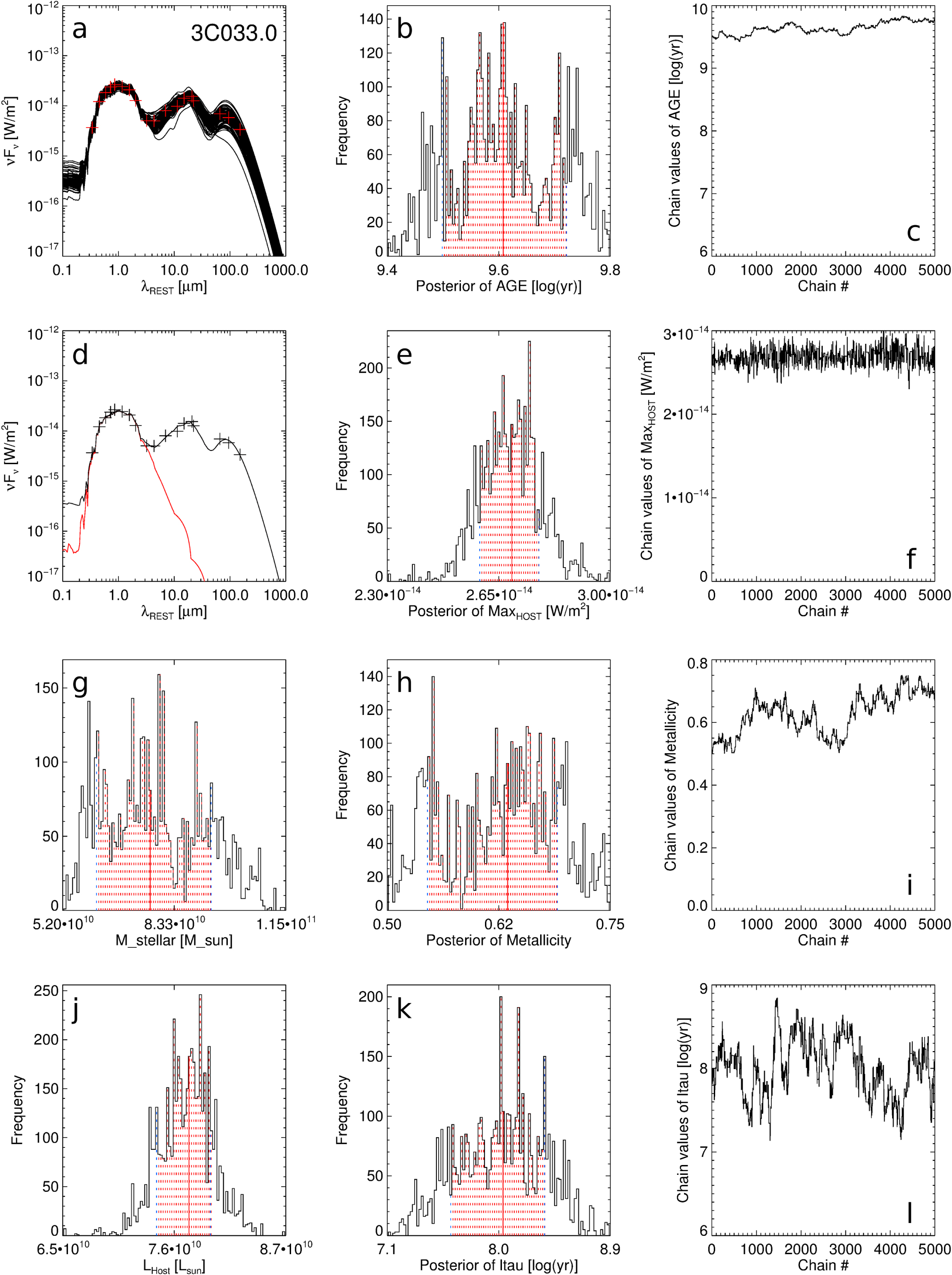
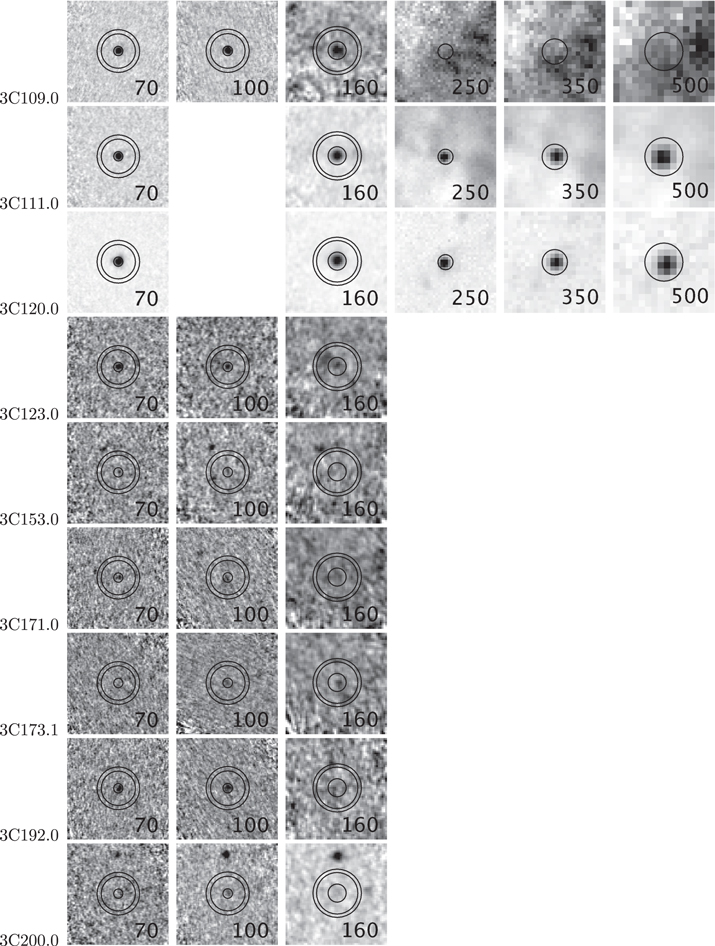
Figure 26. PACS 2', SPIRE 4' stamps of 3C-sources at  .
.
Download figure:
Standard image High-resolution image
Footnotes
- *
Herschel is an ESA space observatory with science instruments provided by European-led Principal Investigator consortia and with important participation from NASA.
- 7
Due to the large ISO beam (FWHM = 90'' at 160 μm), the "high" flux of some 3C-sources (e.g., 3C 20 and 3C 47) contains contributions from nearby sources revealed by our Herschel maps.
- 8
- 9
- 10
- 11
- 12
- 13
- 14