Open AccessArticle

A Novel Three-Parameter Nadarajah Haghighi Model: Entropy Measures, Inference, and Applications

Etaf Alshawarbeh

Fatimah M. Alghamdi

²,

Mohammed Amine Meraou

^3,*

Hassan M. Aljohani

⁴

Mahmoud Abdelraouf

⁵

Fathy H. Riad

⁶,

Sara Mohamed Ahmed Alsheikh

⁷

and

Meshayil M. Alsolmi

⁸

Department of Mathematics, College of Science, University of Ha’il, P.O. Box 55476, Ha’il 55425, Saudi Arabia

Department of Mathematical Sciences, College of Science, Princess Nourah bint Abdulrahman University, P.O. Box 84428, Riyadh 11671, Saudi Arabia

Laboratory of Statistics and Stochastic Processes, University of Djillali Liabes, BP 89, Sidi Bel Abbes 22000, Algeria

⁴

Department of Mathematics and Statistics, College of Science, Taif University, P.O. Box 11099, Taif 21944, Saudi Arabia

⁵

Basic and Applied Science Institute, Arab Academy for Science, Technology and Maritime Transport (AASTMT), Alexandria P.O. Box 1029, Egypt

⁶

Mathematics Department, College of Science, Jouf University, P.O. Box 2014, Sakaka 72388, Saudi Arabia

⁷

Department of Statistics, Faculty of Science, University of Tabuk, P.O. Box 71491, Tabuk 47512, Saudi Arabia

⁸

College of Science and Arts at Khulis, Department of Mathematics, University of Jeddah, Jeddah 22233, Saudi Arabia

Author to whom correspondence should be addressed.

Symmetry 2024, 16(6), 751; https://doi.org/10.3390/sym16060751

Submission received: 11 April 2024 / Revised: 24 May 2024 / Accepted: 11 June 2024 / Published: 16 June 2024

(This article belongs to the Special Issue Symmetric or Asymmetric Distributions and Its Applications)

Download

Browse Figures

Figure 1
A graphical illustration of pdf of the Possible pdf HTNH model. "> Figure 2
A graphical illustration of cdf and sf of the HTNH model: (a) cdf; (b) sf. "> Figure 3
A graphical illustration of hrf of the HTNH model. "> Figure 4
3 dimension plot of the statistical properties at <math display="inline"><semantics> <mrow> <mi>α</mi> <mo>=</mo> <mn>2</mn> </mrow> </semantics></math>. "> Figure 5
3 dimension plot of the statistical properties at <math display="inline"><semantics> <mrow> <mi>α</mi> <mo>=</mo> <mn>4</mn> </mrow> </semantics></math>. "> Figure 6
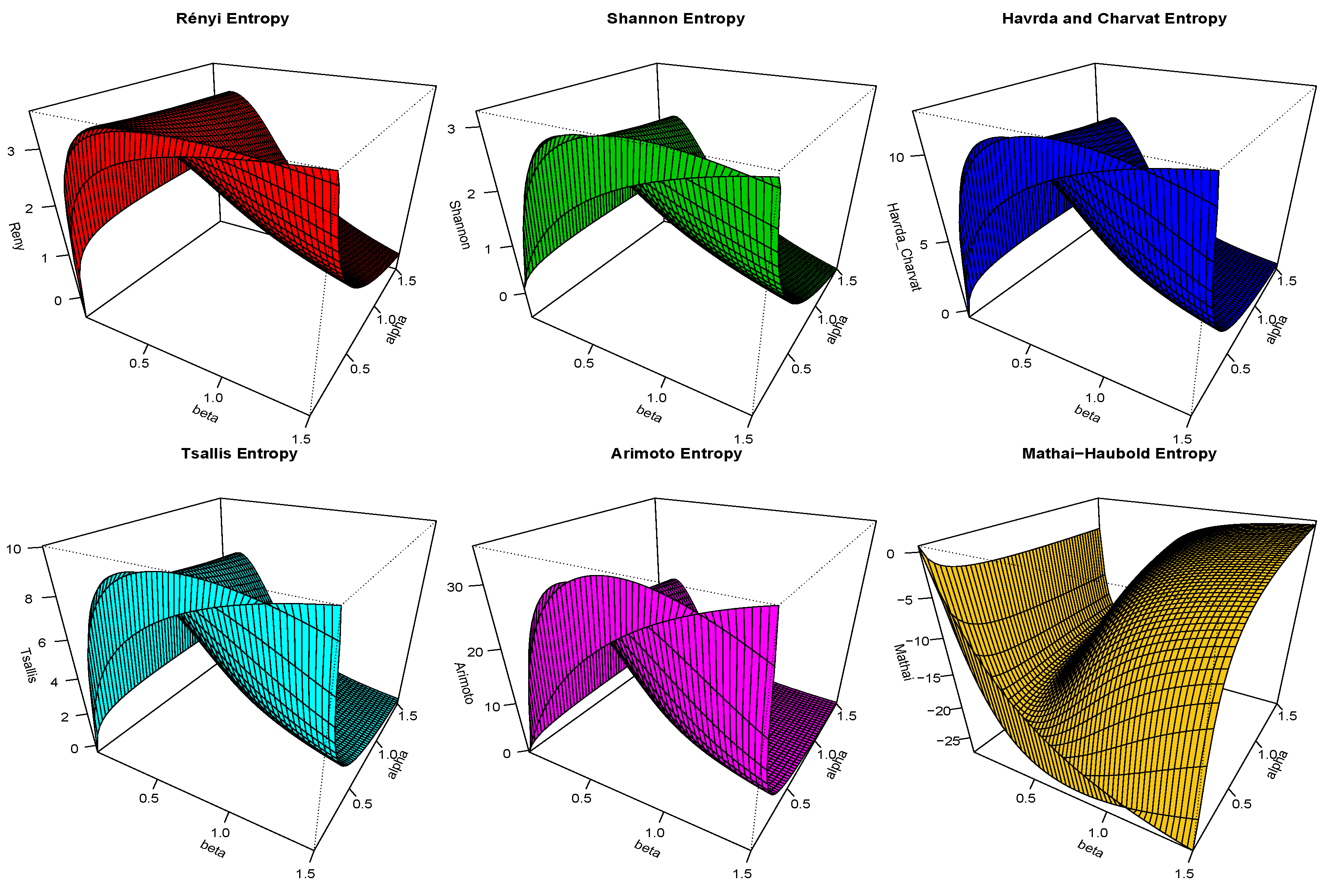
3 dimensions plots of the recommended information measures with <math display="inline"><semantics> <mrow> <mi>λ</mi> <mo>=</mo> <mn>1.5</mn> </mrow> </semantics></math> and <math display="inline"><semantics> <mrow> <mi>τ</mi> <mo>=</mo> <mn>0.5</mn> </mrow> </semantics></math>. "> Figure 7
3 dimensions plots of the recommended information measures with <math display="inline"><semantics> <mrow> <mi>λ</mi> <mo>=</mo> <mn>3</mn> </mrow> </semantics></math> and <math display="inline"><semantics> <mrow> <mi>τ</mi> <mo>=</mo> <mn>1.25</mn> </mrow> </semantics></math>. "> Figure 8
Non-parametric plots of the three proposed datasets. "> Figure 9
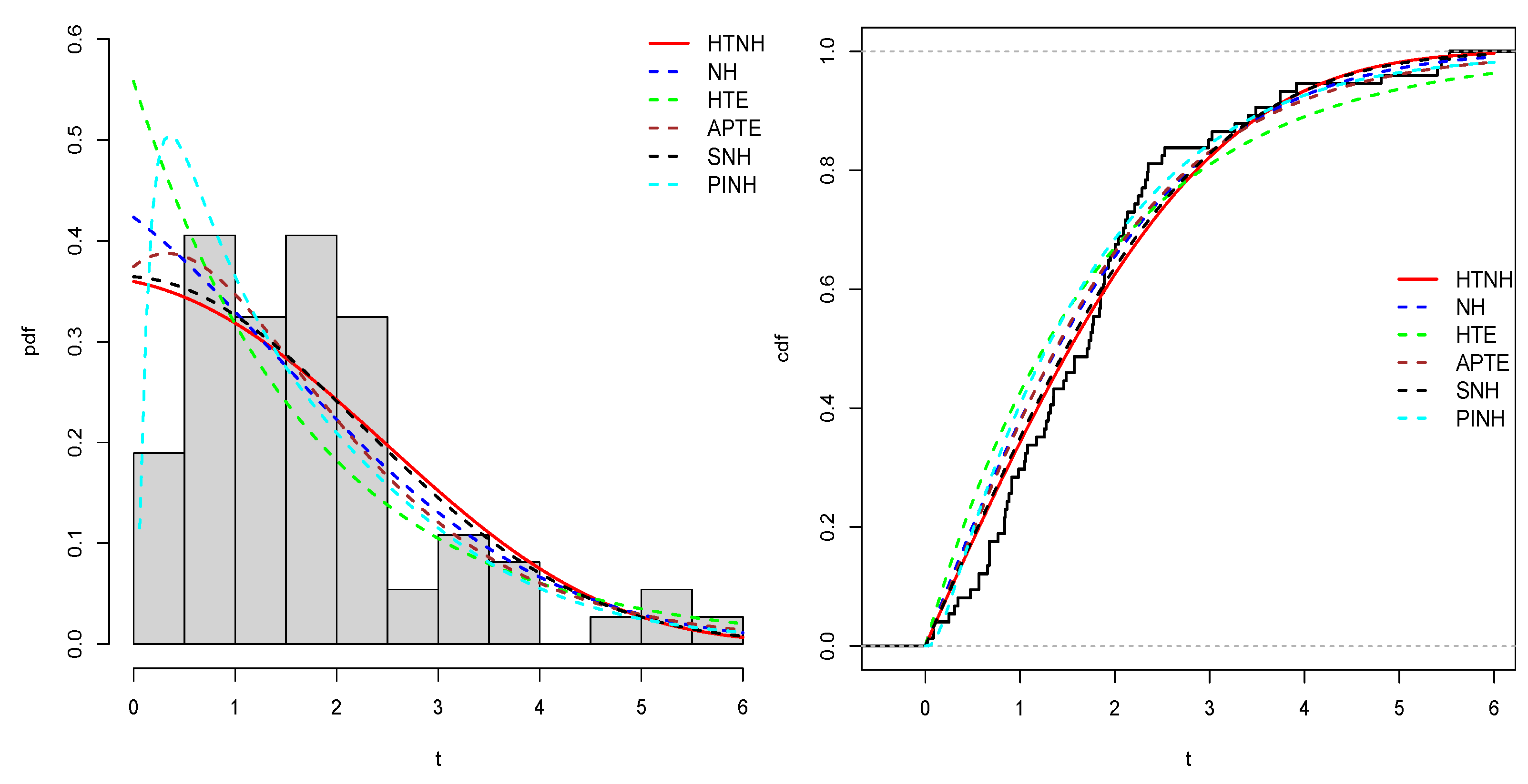
The pdf and cdf estimate plots for the fitting distributions using the first dataset. "> Figure 10
The pdf and cdf estimate plots for the fitting distributions using the second dataset. "> Figure 11
The pdf and cdf estimate plots for the fitting distributions using the third dataset. ">

Versions Notes

Abstract

The fitting and modeling of skewed, complex, symmetric, and asymmetric datasets is an exciting research topic in many fields of applied sciences: notably, lifetime, medical, and financial sciences. This paper introduces a heavy-tailed Nadarajah Haghighi model by compounding the heavy-tailed family and Nadarajah Haghighi distribution. The model obtained has three parameters that account for the scale and shape of the distribution. The proposed distribution’s fundamental characteristics, such as the probability density, cumulative distribution, hazard rate, and survival functions, are provided, several key statistical properties are established, and several entropy information measures are proposed. Estimation of model parameters is performed via a maximum likelihood estimator procedure. Further, different simulation experiments are conducted to demonstrate the proposed estimator’s performance using measures like the average estimate, the average bias, and the associated mean square error. Finally, we apply our proposed model to analyze three different real datasets. In our illustration, we compare the practicality of the recommended model with several well-known competing models.

Keywords:

asymmetric dataset; heavy-tailed; MLE procedure; Nadarajah Haghighi; simulation experiments; survival function; symmetric dataset

1. Introduction

In the last few decades, classical distributions have typically been found to lack fit in many areas of study, such as economics, actuarial science, engineering, environmental science, lifetime, medical science, and several others. Because of this, the authors have elaborated seriously on establishing several distinctive models adapted for specific datasets like symmetrical, asymmetrical, complex, and skewed datasets. This flexibility may be achieved by adding new factors to the classic distribution, including adding one or more parameters or making several transformations to the baseline distribution in order to increase its ability to handle complicated scenarios. In this context, numerous classes of distributions have been obtained by applying different procedures to reinforce the adaptability of models, thereby creating a more versatile and potent distribution for dataset modeling. These suggested families of distributions have an important efficiency in accepting various kinds of data sets, notably asymmetric, bi-modal, and right or left skewed datasets as well as provide greater flexibility for analyzing various applications: for examples, see the studies of Madhavi and Kundu [1], Alfaer er al. [2], Marshall and Olkin [3], Afify et al. [4], Meraou and Raqab [5], Ahmad et al. [6], Meraou el al. [7], Gemeay et al. [8], Amal S. Hassan et al. [9], Sapkota et al. [10], Cordeiro et al. [11], Teamah et al. [12], Bourguignon et al. [13], Yıldırım et al. [14], Meraou et al. [15], Almuqrin et al. [16], Zagrofos and Balakrishana [17], Kamal et al. [18], Teamah et al. [19], Eugene et al. [20], Alsadat et al. [21], Alzaatreh et al. [22], Nagy et al. [23], and Meraou et al. [24].

Recently, a novel class of distributions was provided by Ahmed et al. [25] called the heavy-tailed (HT) class of distributions. This new extension is an appropriate model for modeling HT, symmetric, complex, and skewed datasets, and it is a powerful method for generating new models to analyze datasets’ underlying patterns better. The HT class of distributions can portray several real–realistic application studies in many areas, notably hydrology, biology, agriculture, production, survival, and finance. The cdf and pdf of the HT family of distributions can be expressed, respectively, as follows:

F (y) = \frac{λ K (y)}{λ - 1 + K (y)}, y \in R, λ > 1,

(1)

and

f (y) = \frac{λ (λ - 1) k (y)}{{[λ - 1 + K (y)]}^{2}},

(2)

where

K (y)

and

k (y)

represent respectively density and cumulative distribution of the baseline model. Now, the survival function (sf) with corresponding hazard rate function (hrf) of the proposed HT class of distributions are expressed, respectively, as

S (y) = \frac{(λ - 1) (1 - K (y))}{λ - 1 + K (y)}, y \in R, λ > 1,

(3)

and

h (y) = \frac{λ (λ - 1) k (y)}{S (y) {[λ - 1 + K (y)]}^{2}},

(4)

It is well documented that the Nadarajah Haghighi (NH) model is widely used in statistical modeling. It is an innovative extension of the exponential distribution that serves as an alternative model to the gamma and exponentiated–exponential distribution. The NH distribution was first introduced by Nadarajah and Haghighi [26], and it can be applied to fit several kinds of datasets—notably, skewed, complex, and heavy-tailed—and it can also be used in different fields of application, particularly in reliability and engineering. It is well-documented that the NH model can be extensively investigated in many study domains. Noteworthy studies involving this model include Almetwally and Meraou [27], Korkmaz et al. [28], Salama et al. [29], Almongy et al. [30], Tahir et al. [31], Lone et al. [32], Shafq et al. [33], and Anum Shafiq et al. [34]. The cdf and pdf of an NH distribution are formulated, respectively, as

\begin{matrix} G (y) & = 1 - e^{1 - {(1 + β y)}^{α}}, y, α, β > 0, \end{matrix}

(5)

and

\begin{matrix} g (y) & = α β {(1 + β y)}^{α - 1} e^{1 - {(1 + β y)}^{α}}, \end{matrix}

(6)

where

α

and

β

represent the shape and scale parameters, respectively. These two parameters show the non-monotone shape of the hazard rate and the failure times of components and systems.

This research aims to enhance the NH distribution, resulting in a generalized distribution termed the heavy-tailed Nadarajah Haghighi model (HTNH). The model’s flexibility is obtained by a new additional shape parameter that defines its cumulative distribution function. The additional parameter plays an important role in analyzing the tail behavior of the proposed density function. Also, the newly added parameter efficiently models many reliability functions, such as the hazard rate function, and can be used to fit skewed datasets. This distribution can find a wide range of applications in analyzing business failure lifetime data, sizes of cities, income and wealth inequality, actuarial sciences, medical and biological sciences, engineering, lifetime, and reliability. The pdf of the proposed model can be decreased and skewed, and a sub-model can be obtained as a special case. Estimation of the model’s parameters is performed via the maximum likelihood estimator (MLE) and Bayes techniques. It is worth mentioning that the Bayesian method is performed via the square error loss function. Many applications for this method have been found by researchers, including Xu et al. [35], Almetwally et al. [36], Al-Babtain et al. [37], and Zhou et al. [38]. Further, we introduce a confidence interval (CI) for the model parameters by using the asymptotic distribution of the MLE procedure, and various entropy information measures are introduced.

The following factors were involved in the design of this paper. In Section 2, we define our HTNH model and established its distributional properties. Many mathematical properties of our proposed model are provided in Section 3. The final expressions of six proposed entropy information measures for the HTNH model are formulated in Section 4. Section 5 demonstrates the estimation of model parameters via the MLE technique, and the CIs of unknown parameters for our HTNH model are also constructed in this section. In Section 6, a Monte Carlo (MC) simulation analysis is illustrated to show the consistency and unbiasedness of the recommended estimator, and three real datasets are utilized to select the more appropriate distributions in Section 7. Finally concluding results are provided for this study in the last section.

2. The HTNH Model and Its Distributional Properties

In this part of the work, we consider certain distributional properties of the proposed HTNH model, including the cdf, pdf, sf, hrf, cumulative hrf (chrf), and reverse hrf (rhrf).

Theorem 1.

Let T be a random variable following the HTNH model with parameters λ, α, and β (

T \sim

HTNH

(λ, α, β)

). According to Equations (1) and (5), the cdf and pdf of T are obtained, and they are expressed, respectively, as follows:

\begin{matrix} Δ (t) & = \frac{λ [1 - e^{1 - {(1 + β t)}^{α}}]}{λ - e^{1 - {(1 + β t)}^{α}}}, t > 0, and, λ > 1, α, β > 0, \end{matrix}

(7)

and

\begin{matrix} δ (t) & = \frac{α β λ (λ - 1) {(1 + β t)}^{α - 1} e^{1 - {(1 + β t)}^{α}}}{{[λ - e^{1 - {(1 + β t)}^{α}}]}^{2}} . \end{matrix}

(8)

The limiting behavior of the pdf of the recommended HTNH model if

t \to 0

and

t \to + \infty

can be expressed as

lim_{t \to 0} δ (t) = \frac{α β λ}{λ - 1} and lim_{t \to + \infty} δ (t) = 0

Consequently, for all parameter values of λ, α, and β, the pdf of the HTNH distribution is decreasing.

Under Equation (7), the HT exponential (HTE) distribution can be obtained as a special case when α = 1. Figure 1 depicts a few of the most likely contours of the pdf using several parameter values of HTNH distribution. In all situations, the pdf of the suggested HTNH model is decreasing and is positively skewed.

Theorem 2.

The sf and hrf of T are structured, respectively, by

S (t) = \frac{e^{1 - {(1 + β t)}^{α}} (λ - 1)}{λ - e^{1 - {(1 + β t)}^{α}}},

and

h (t) = \frac{α β λ m {(1 + β t)}^{α - 1}}{λ - e^{1 - {(1 + β t)}^{α}}} .

The plots of the cdf and sf of the HTNH model are sketched in Figure 2, while Figure 3 depicts the graphs of the hrf curves of the proposed HTNH distribution. From Figure 3, the hrf of the HTNH distribution has different forms. It is increase, decrease, and J-forms curves. Consequently, it can be deduced that our HTNH distribution is and efficient model in analyzing numerous types of datasets.

Theorem 3.

The chrf and rhrf of the HTNH model are written, respectively, as

\begin{matrix} H (t) = & - log \{\frac{e^{1 - {(1 + β t)}^{α}} (λ - 1)}{λ - e^{1 - {(1 + β t)}^{α}}}\}, \end{matrix}

and

R (t) = \frac{α β (λ - 1) {(1 + β t)}^{α} e^{1 - {(1 + β t)}^{α}}}{(λ - e^{1 - {(1 + β t)}^{α}}) (1 - e^{1 - {(1 + β t)}^{α}})} .

3. Statistical Properties of HTNH Model

In this part of the study, we establish several mathematical properties of the proposed HTNH model. In this subsection, let us consider

T \sim H T N H (λ, α, β)

3.1. Identifiability Property

The parameter

λ

is applied to provide the identifiability property of the proposed HTNH model, which is useful for making precise inferences. Suppose that

λ_{1}

and

λ_{2}

follow the cdf as described in (7). The parameter

λ

is identifiable if

λ_{1} = λ_{2}

. As a result,

\begin{matrix} Δ (t; λ_{1}) & = & Δ (t; λ_{2}) \\ \frac{λ_{1} [1 - e^{1 - {(1 + β t)}^{α}}]}{λ_{1} - e^{1 - {(1 + β t)}^{α}}} & = & \frac{λ_{2} [1 - e^{1 - {(1 + β t)}^{α}}]}{λ_{2} - e^{1 - {(1 + β t)}^{α}}} \\ λ_{1} λ_{2} - λ_{1} e^{1 - {(1 + β t)}^{α}} - λ_{1} λ_{2} e^{1 - {(1 + β t)}^{α}} - λ_{1} e^{2 (1 - {(1 + β t)}^{α})} & = & λ_{2} λ_{1} - λ_{2} e^{1 - {(1 + β t)}^{α}} - λ_{2} λ_{1} e^{1 - {(1 + β t)}^{α}} - λ_{2} e^{2 (1 - {(1 + β t)}^{α})} \\ - λ_{1} e^{1 - {(1 + β t)}^{α}} - λ_{1} e^{2 (1 - {(1 + β t)}^{α})} & = & - λ_{2} e^{1 - {(1 + β t)}^{α}} - λ_{2} e^{2 (1 - {(1 + β t)}^{α})} \\ λ_{1} (1 - e^{1 - {(1 + β t)}^{α}}) (λ_{2} - e^{1 - {(1 + β t)}^{α}}) & = & λ_{2} (1 - e^{1 - {(1 + β t)}^{α}}) (λ_{1} - e^{1 - {(1 + β t)}^{α}}) \\ λ_{1} (e^{2 (1 - {(1 + β t)}^{α})} + e^{1 - {(1 + β t)}^{α}}) & = & λ_{2} (e^{2 (1 - {(1 + β t)}^{α})} + e^{1 - {(1 + β t)}^{α}}) \\ λ_{1} & = & λ_{2} \end{matrix}

3.2. Quantile Function

Theorem 4.

The quantile function of T can be formulated by

{QF}_{q} = \frac{1}{β} \{{(1 - log [\frac{λ (q - 1)}{q - λ}])}^{\frac{1}{α}} - 1\} 0 < q < 1 .

(9)

Using the above equation, a random sample from our suggested HTNH model may be generated with q following a uniform random number (0,1), which will be useful for further development.

The coefficients for the skewness (

SK

) and kurtosis (

KR

) of T can be formulated, respectively, as

SK = \frac{{QF}_{1 / 4} + {QF}_{3 / 4} - 2 {QF}_{1 / 2}}{{QF}_{3 / 4} - {QF}_{1 / 4}},

and

KR = \frac{{QF}_{7 / 8} - {QF}_{5 / 8} + {QF}_{3 / 8} - {QF}_{1 / 8}}{{QF}_{6 / 8} - {QF}_{2 / 8}} .

3.3. Useful Expansion

The expansion of the proposed pdf of the HTNH model is

δ (t) = \frac{λ (λ - 1) g (t)}{{[λ - 1 + G (t)]}^{2}},

where

G (t)

and

g (t)

are given in Equations (5) and (6), respectively.

\begin{matrix} δ (t) & = & \frac{λ (λ - 1) g (t)}{{[(λ - 1) (1 + \frac{G (t)}{λ - 1})]}^{2}} \\ = & \frac{λ (λ - 1) g (t)}{{(λ - 1)}^{2} {[1 + \frac{G (t)}{λ - 1}]}^{2}} \\ = & \frac{λ g (t)}{(λ - 1) {[1 + \frac{G (t)}{λ - 1}]}^{2}} \end{matrix}

For simplicity, we utilize the negative binomial series:

{(ρ + a)}^{- n} = \sum_{m = 0}^{\infty} {(- 1)}^{m} (\binom{n + m - 1}{m}) ρ^{m} a^{- n - m}, ∣ ρ ∣ < a .

Now, by taking

a = 1

and

n = 2

, we obtain

{(ρ + 1)}^{- 2} = \sum_{m = 0}^{\infty} {(- 1)}^{m} (\binom{m + 1}{m}) ρ^{m} .

The pdf of the recommended HTNH model can be rewritten as

\begin{matrix} δ (t) & = & \sum_{m = 0}^{\infty} {(- 1)}^{m} (\binom{m + 1}{m}) \frac{λ}{(λ - 1) {(λ - 1)}^{m}} g (t; α, β) {[G (t; α, β)]}^{m} \\ = & \sum_{m = 0}^{\infty} {(- 1)}^{m} (\binom{m + 1}{m}) \frac{λ}{{(λ - 1)}^{m + 1}} g (t) {[G (t)]}^{m} \end{matrix}

By substituting

G (t; α, β)

and

g (t; α, β)

as the cdf and pdf, respectively, of the NH distribution, the pdf of the proposed HTNH model is defined by Equation (10). It is given by

\begin{matrix} δ (t) & = & \sum_{m = 0}^{\infty} {(- 1)}^{m} (\binom{m + 1}{m}) \frac{α β λ}{{(λ - 1)}^{m + 1}} {(1 + β t)}^{α - 1} e^{1 - {(1 + β t)}^{α}} {(1 - e^{1 - {(1 + β t)}^{α}})}^{m} . \end{matrix}

(10)

Similarly, the cumulative distribution of the recommended HTNH model is rewritten as

\begin{matrix} Δ (t) & = & \frac{λ G (t)}{λ - 1 + G (t)} \\ = & \frac{λ G (λ - 1 + G (t))}{{[λ - 1 + G (t)]}^{2}} \\ = & \frac{λ G (t) (λ - 1) (1 + \frac{G (t)}{λ - 1})}{{(λ - 1)}^{2} {[1 + \frac{G (t)}{λ - 1}]}^{2}} \\ = & \frac{λ G (t)}{(λ - 1) [1 + \frac{G (t)}{λ - 1}]} \end{matrix}

Using a negative binomial series with

{(ρ + 1)}^{- 1} = \sum_{m = 0}^{\infty} {(- 1)}^{m} ρ^{m},

the cdf of the proposed HTNH model can be rewritten as

\begin{matrix} = & \sum_{m = 0}^{\infty} {(- 1)}^{m} \frac{λ}{(λ - 1) {(λ - 1)}^{m}} G (t) {[G (t)]}^{m} \\ = & \sum_{m = 0}^{\infty} {(- 1)}^{m} \frac{λ}{{(λ - 1)}^{m + 1}} {[G (t)]}^{m + 1} \end{matrix}

By substituting

G (t; α, β)

and

g (t; α, β)

as the cdf and pdf, respectively, of NH distribution, the cdf of the proposed HTNH model is defined by Equation (11). It can be written as

\begin{matrix} Δ (t) & = & \sum_{m = 0}^{\infty} {(- 1)}^{m} \frac{λ}{{(λ - 1)}^{m + 1}} {(1 - e^{1 - {(1 + β t)}^{α}})}^{m + 1} . \end{matrix}

(11)

3.4. Moment and Related Measures

Theorem 5.

The corresponding

r t h

moment of T is

u_{r}^{'} = \sum_{m = 0}^{\infty} {(- 1)}^{m} (\binom{m + 1}{m}) \frac{λ}{{(λ - 1)}^{m + 1}} η_{r, α, β} (t),

(12)

where

η_{r, α, β} (t) = \int_{0}^{\infty} α β t^{r} {(1 + β t)}^{α - 1} e^{1 - {(1 + β t)}^{α}} {(1 - e^{1 - {(1 + β t)}^{α}})}^{m} d t

Using Equation (12), the first and second moments of T can be found, and they are written as

u_{1}^{'} = \sum_{m = 0}^{\infty} {(- 1)}^{m} (\binom{m + 1}{m}) \frac{λ}{{(λ - 1)}^{m + 1}} η_{1, α, β} (t)

and

u_{2}^{'} = \sum_{m = 0}^{\infty} {(- 1)}^{m} (\binom{m + 1}{m}) \frac{λ}{{(λ - 1)}^{m + 1}} η_{2, α, β} (t) .

Furthermore, the variance and index of dispersion for T are

V a r (T) = u_{2}^{'} - u_{1}^{' 2}

and

I D = \frac{v a r (Y)}{u_{1}^{'}} .

Theorem 6.

Based on [39], the moment-generating function (mgf) is presented as follows:

M (y) = \sum_{r = 0}^{\infty} \sum_{m = 0}^{\infty} {(- 1)}^{m} (\binom{m + 1}{m}) \frac{λ y^{r}}{{(λ - 1)}^{m + 1} r!} η_{r, α, β} (t) .

Theorem 7.

The corresponding characteristic function (cf) of T is

Φ (y) = \sum_{r = 0}^{\infty} \sum_{m = 0}^{\infty} {(- 1)}^{m} (\binom{m + 1}{m}) \frac{λ {(i y)}^{r}}{{(λ - 1)}^{m + 1} r!} η_{r, α, β} (t) .

Table 1 and Table 2 represent several suggested statistical properties of the HTNH model, like

u_{1}^{'}

, variance, ID,

K

, and

R

, which are also displayed in Figure 4 and Figure 5.

3.5. Residual and Reverse Residual Life

Theorem 8.

Let T be a random variable that follows the HTNH model. The residual reliability function of Y, abbreviated as

D_{l} (t)

, can be defined as

\begin{matrix} D_{l} (t) & = & \frac{S (t + l)}{S (l)} \\ = & \frac{(1 - G (t + l)) (λ - 1 + G (l))}{[1 - G (l)] [λ - 1 + G (t + l)]} \\ = & \frac{e^{1 - {(1 + β (t + l))}^{α}} (λ - e^{1 - {(1 + β l)}^{α}})}{e^{1 - {(1 + β l)}^{α}} (λ - e^{1 - {(1 + β (t + l))}^{α}})} . \end{matrix}

Theorem 9.

The reverse residual reliability function of Y, abbreviated as

{\bar{D}}_{l} (t)

, is

\begin{matrix} {\bar{D}}_{l} (t) & = & \frac{S (t - l)}{S (l)} \\ = & \frac{(1 - G (t - l)) (λ - 1 + G (l))}{[1 - G (l)] [λ - 1 + G (t - l)]} \\ = & \frac{e^{1 - {(1 + β (t - l))}^{α}} (λ - e^{1 - {(1 + β l)}^{α}})}{e^{1 - {(1 + β l)}^{α}} (λ - e^{1 - {(1 + β (t - l))}^{α}})} . \end{matrix}

3.6. The Pdf and Cdf of the Order Statistics of the HTNH Model

Assume that

T_{1}, T_{2}, \dots, T_{n}

is a random sample taken from the HTNH distribution, and

T_{(1 : n)}, T_{(2 : n)}, \dots, T_{(n : n)}

represents its order statistics. Further, the

j t h

pdf of

T_{(j : n)}

\begin{matrix} ψ_{(j : n)} (t) & = & \frac{n!}{(j - 1)! (n - j)!} δ (t) {[Δ (t)]}^{j - 1} {[1 - Δ (t)]}^{n - j} \\ = & \frac{α β λ (λ - 1) n! {(1 + β t)}^{α - 1} e^{1 - {(1 + β t)}^{α}}}{(j - 1)! (n - j)!} {(λ - e^{1 - {(1 + β t)}^{α}})}^{j - 3} {(λ [1 - e^{1 - {(1 + β t)}^{α}}])}^{j - 1} \\ \times & {(1 - \frac{λ [1 - e^{1 - {(1 + β t)}^{α}}]}{λ - e^{1 - {(1 + β t)}^{α}}})}^{n - j} . \end{matrix}

The corresponding

j^{t h}

cdf of

T_{(j : n)}

can be provided as

\begin{matrix} Ψ_{(j : n)} (t) & = & \sum_{i = j}^{n} Δ^{i} (t) {[1 - Δ (t)]}^{n - i} \\ = & \sum_{i = j}^{n} \sum_{w = 0}^{n - i} (\binom{n}{i}) (\binom{n - i}{w}) {(- 1)}^{i} Δ^{w + i} (t) \\ = & \sum_{i = j}^{n} \sum_{w = 0}^{n - i} (\binom{n}{i}) (\binom{n - i}{w}) {(- 1)}^{i} {(\frac{λ [1 - e^{1 - {(1 + β t)}^{α}}]}{λ - e^{1 - {(1 + β t)}^{α}}})}^{w + i} . \end{matrix}

Hence, the pdfs of the

T_{(1 : n)}

and

T_{(n : n)}

, defined, respectively, as

T_{(n : n)} = max {t_{1}, t_{2}, \dots, t_{n}}

and

T_{(1 : n)} = min {t_{1}, t_{2}, \dots, t_{n}}

, are written as

\begin{matrix} ψ_{(1 : n)} (t) & = & n α β λ (λ - 1) {(1 + β t)}^{α - 1} e^{1 - {(1 + β t)}^{α}} {(λ - e^{1 - {(1 + β t)}^{α}})}^{- 2} {(1 - \frac{λ [1 - e^{1 - {(1 + β t)}^{α}}]}{λ - e^{1 - {(1 + β t)}^{α}}})}^{n - 1}, \end{matrix}

and

\begin{matrix} ψ_{(n : n)} (t) & = & n α β λ (λ - 1) {(1 + β t)}^{α - 1} e^{1 - {(1 + β t)}^{α}} {(λ - e^{1 - {(1 + β t)}^{α}})}^{n - 3} {(λ [1 - e^{1 - {(1 + β t)}^{α}}])}^{n - 1} . \end{matrix}

4. Certain Entropy Measures

This subsection considers numerous information entropy measures: notably, Rényi, Shannon, Havrda and Charvat, Tsallis, Arimoto, and Mathai–Haubold.

First, we started with the Rényi [40]

(Ξ_{1} (τ)

) entropy of our HTNH model. The Renyi entropy is a measure of uncertainty in information theory. It is formulated by

\begin{matrix} Ξ_{1} (τ) & = & \frac{1}{1 - τ} log (\int_{0}^{\infty} δ^{τ} (t) d t) τ \neq 1, τ > 0 . \\ = & \frac{1}{1 - τ} log ({\{\int_{0}^{\infty} \sum_{m = 1}^{\infty} \frac{{(- 1)}^{m - 1} m λ α β}{{(λ - 1)}^{m}} e^{1 - {(1 + η t)}^{α}} {(1 + β t)}^{α - 1} {(1 - e^{1 - {(1 + β t)}^{α}})}^{m - 1} d t\}}^{τ}) \\ = & \frac{{(λ α β)}^{τ}}{1 - τ} log ({\{\sum_{m = 1}^{\infty} \frac{{(- 1)}^{m - 1} m}{{(λ - 1)}^{m}} Φ_{m, α, β} (t)\}}^{τ}), \end{matrix}

with

Φ_{m, α, β} (t) = \int_{0}^{\infty} e^{1 - {(1 + β t)}^{α}} {(1 + β t)}^{α - 1} {(1 - e^{1 - {(1 + β t)}^{α}})}^{m - 1} d t

The Shannon entropy is another information uncertainty measure. It is simply the “amount of information” in a variable, defined as

\begin{matrix} Ξ_{2} & = & E (- log δ (t)) \\ = & E (- log [\frac{α β λ (λ - 1) {(1 + β t)}^{α - 1} e^{1 - {(1 + β t)}^{α}}}{{[λ - e^{1 - {(1 + β t)}^{α}}]}^{2}}]) \\ = & - log (α β λ (λ - 1)) - (α - 1) E (log [1 + β t]) - E (1 - {(1 + β t)}^{α}) + 2 E (log [λ - e^{1 - {(1 + β t)}^{α}}]) \end{matrix}

Next, we consider the novel Havrda and Charvat entropy [41] (

Ξ_{3} (τ)

) of the proposed HTNH distribution in this work. The Havrda and Charvat entropy represents a parametric extension of the Shannon entropy. We propose to use this information to get a better grasp on all sorts of data.

It is presented as

\begin{matrix} Ξ_{3} (τ) & = & \frac{1}{2^{1 - τ} - 1} (\int_{0}^{\infty} δ (t) d t - 1) τ \neq 1, τ > 0 . \\ = & \frac{α β λ}{2^{1 - τ} - 1} (\sum_{m = 1}^{\infty} \frac{{(- 1)}^{m - 1} m}{{(λ - 1)}^{m}} Φ_{m, α, β} (t) - 1) . \end{matrix}

The Tsallis entropy [42]

Ξ_{4} (τ)

(also used bu Ibrahim [43]) is proportional to the expectation of the

τ

-logarithm of the HTNH distribution. It can be written as

\begin{matrix} Ξ_{4} (τ) & = & \frac{1}{1 - τ} (1 - \int_{0}^{\infty} δ^{τ} (t) d t) τ \neq 1, τ > 0 . \\ = & \frac{{(λ α β)}^{τ}}{τ - 1} (1 - {\{\sum_{m = 1}^{\infty} \frac{{(- 1)}^{m - 1} m}{{(λ - 1)}^{m}} Φ_{m, α, β} (t)\}}^{τ}) . \end{matrix}

Further, we express the Arimoto entropy [44] (

Ξ_{5} (τ)

) of the HTNH model, which is a generalization of the Shannon entropy. It is a similarity metric used to measure statistical dependence. It can be examined by

\begin{matrix} Ξ_{5} (τ) & = & \frac{τ}{1 - τ} (\int_{0}^{\infty} {\{δ^{τ} (t) d t\}}^{\frac{1}{τ}} - 1) τ \neq 1, τ > 0 . \\ = & \frac{λ α β τ}{τ - 1} ({\{\sum_{m = 1}^{\infty} \frac{{(- 1)}^{m - 1} m}{{(λ - 1)}^{m}} Φ_{m, α, β} (t)\}}^{\frac{1}{τ}} - 1) . \end{matrix}

In the end, a novel flexible information called the Mathai–Haubold entropy [45] (

Ξ_{6} (τ)

) is established. It can be used in residual lifetime and engineering applications. It can be defined as follows:

\begin{matrix} Ξ_{6} (τ) & = & \frac{1}{τ - 1} (\int_{0}^{\infty} δ^{2 - τ} (t) d t - 1) τ \neq 1, τ > 0 . \\ = & \frac{{(λ α β)}^{2 - τ}}{τ - 1} ({\{\sum_{m = 1}^{\infty} \frac{{(- 1)}^{m - 1} m}{{(λ - 1)}^{m}} Φ_{m, α, β} (t)\}}^{2 - τ} - 1) . \end{matrix}

Table 3 and Table 4 summarize certain information entropy measures of the HTNH model as discussed in this section using several selected parameters of

λ

α

, and

β

. Further, Figure 6 and Figure 7 depict the 3D curves of these information entropy measures. It is clear from the results in Table 3 and Table 4 that:

When $α$ increases and $β$ and $λ$ are fixed, the values of $Ξ_{1} (τ), Ξ_{2}, Ξ_{3} (τ), Ξ_{4} (τ),$ and $Ξ_{5} (τ)$ tend to decrease, whereas the value of $Ξ_{6} (τ)$ increases.
When $β$ increases and $α$ and $λ$ are fixed, we obtain the same results.
Finally, if $τ$ increases, the values of $Ξ_{1} (τ), Ξ_{2},$ and $Ξ_{6}$ increase, but the values of $Ξ_{3} (τ), Ξ_{4},$ and $Ξ_{5}$ decrease.
The HTNH model has a great role in modeling different fields of datasets.

5. Statistical Inference

In this section, we introduce different estimator techniques for determining the estimate parameters of our proposed model.

5.1. Maximum Likelihood Estimator

Assume that

(t_{1}, t_{2} \dots, t_{n})

is a random sample drawn from our HTNH model of size n, and let

Θ = (λ, α, β)

denote the parameter vector. The log-likelihood function of our model can be written as follows:

\begin{matrix} LL (Θ) & = & n log α + n log β + n log λ + n log (λ - 1) + (α - 1) \sum_{i = 1}^{n} log (1 + β t_{i}) + \sum_{i = 1}^{n} (1 - {(1 + β t_{i})}^{α}) \\ - & 2 \sum_{i = 1}^{n} log (λ - e^{1 - (1 + β t_{i}) α}) . \end{matrix}

(13)

The partial derivatives of Equation (13) with their respective parameters are

\frac{\partial LL (Θ)}{\partial λ} = \frac{n}{λ} + \frac{n}{λ - 1} - 2 \sum_{i = 1}^{n} {(λ - e^{1 - (1 + β t_{i}) α})}^{- 1},

(14)

\frac{\partial LL (Θ)}{\partial α} = \frac{n}{α} + \sum_{i = 1}^{n} log (1 + β t_{i}) - \sum_{i = 1}^{n} {(1 + β t_{i})}^{α} log {(1 + β t_{i})}^{α} - 2 \sum_{i = 1}^{n} \frac{{(1 + β t_{i})}^{α} e^{1 - {(1 + β t_{i})}^{α}}}{λ - e^{1 - (1 + β t_{i}) α}},

(15)

and

\frac{\partial LL (Θ)}{\partial β} = \frac{n}{β} + (α - 1) \sum_{i = 1}^{n} t_{i} {(1 + β t_{i})}^{- 1} - α \sum_{i = 1}^{n} t_{i} {(1 + β t_{i})}^{α - 1} - 2 α \sum_{i = 1}^{n} \frac{t_{i} {(1 + β t_{i})}^{α - 1} e^{1 - {(1 + β t_{i})}^{α}}}{λ - e^{1 - (1 + β t_{i}) α}} .

(16)

Equations (14)–(16) describe non-linear equations that are tricky to write concisely, rendering it difficult to solve them directly for the vector parameter

Θ = (λ, α, β)

. Iterative approaches, notably fixed-point, secant, and Newton–Raphson methods, are employed. The aforementioned methods enable quicker determination of the MLE of

LL (Θ)

. We note that all obtained estimates of the proposed HTNH distribution exist and are unique.

5.2. Approximate Confidence Interval

Now to construct the confidence intervals (CIs) of the parameters, by applying the idea of Louis [46], the asymptotic distribution of the MLE of

Θ

is described as

(\hat{Θ} - Θ) \overset{d}{\to} N_{3} (0, J^{- 1} (Θ)),

with

I^{- 1} (Θ)

denotes the inverse of the matrix of

Θ

. The elements of

I^{- 1} (Θ)

are

J^{- 1} (Θ) = (\begin{matrix} \frac{\partial^{2} LL (Θ)}{\partial λ^{2}} & \frac{\partial^{2} LL (Θ)}{\partial λ \partial α} & \frac{\partial^{2} LL (Θ)}{\partial λ \partial β} \\ \frac{\partial^{2} LL (Θ)}{\partial β \partial λ} & \frac{\partial^{2} LL (Θ)}{\partial β^{2}} & \frac{\partial^{2} LL (Θ)}{\partial β \partial α} \\ \frac{\partial^{2} LL (Θ)}{\partial α \partial λ} & \frac{\partial^{2} LL (Θ)}{\partial α \partial β} & \frac{\partial^{2} LL (Θ)}{\partial α^{2}} \end{matrix})

Finally, with

Θ_{1} = λ

Θ_{2} = α

, and

Θ_{3} = β

, the

(1 - γ) %

CI of

Θ_{k}

are

LCB = {\hat{Θ}}_{k} - z_{γ / 2} \sqrt{J^{- 1} ({\hat{Θ}}_{k})}, k = 1, 2, 3,

and

UCB = {\hat{Θ}}_{k} + z_{γ / 2} \sqrt{J^{- 1} ({\hat{Θ}}_{k})}, k = 1, 2, 3,

where LCL is the lower confidence limit, UCL is the upper confidence limit,

z_{γ / 2}

is the upper

γ / 2

quantile of the standard normal distribution,

N (0, 1)

Please see the elements of matrix

J^{- 1} (Θ)

in Appendix A.

5.3. Bayesian Estimator

We suppose that the parameters

λ

α

, and

β

are random variables that have, respectively, the prior pdf gamma distribution, and they are written as follows:

π_{1} (λ) = \frac{b_{1}^{a_{1}}}{Γ (a_{1})} λ^{a_{1} - 1} e^{- b_{1} λ}, λ, a_{1}, b_{1} > 0,

π_{2} (α) = \frac{b_{2}^{a_{2}}}{Γ (a_{2})} α^{a_{2} - 1} e^{- b_{2} α}, α, a_{2}, b_{2} > 0,

and

π_{3} (β) = \frac{b_{3}^{a_{3}}}{Γ (a_{3})} β^{a_{3} - 1} e^{- b_{3} β}, β, a_{3}, b_{3} > 0 .

The joint density is

π (λ, α, β) \propto λ^{a_{1} - 1} β^{a_{2} - 1} e^{- b_{1} λ - b_{2} λ} .

(17)

Further, the posterior density of

λ

α

β

, and the complete samples is given by

\begin{matrix} π^{*} (λ, α, β ∣ z) & = & L (λ, α, β) π (λ, α, β) \\ = & λ^{n + a_{1} - 1} α^{n + a_{2} - 1} β^{n + a_{3} - 1} {(λ - 1)}^{n} e^{- b_{1} λ - b_{2} α - b_{3} β} \prod_{i = 1}^{n} \frac{{(1 + β t_{i})}^{α - 1} e^{1 - {(1 + β t_{i})}^{α}}}{{[λ - e^{1 - {(1 + β t_{i})}^{α}}]}^{2}} . \end{matrix}

With

Θ = (λ, α, β)

, the Bayes estimator of the function of parameters based on the square error (SE) loss function

R = {(Θ - \hat{Θ})}^{2}

is written as

{\hat{R}}_{S E} = \int_{Θ} R π^{*} (Θ ∣ t) d Θ .

(18)

6. Simulation Experiments

We performed Monte Carlo (MC) simulation experiments in this subsection to demonstrate the potential of the MLE and Bayes methods of our suggested HTNH model using several sample sizes

n = {50, 100, 300, 500, 700, 1000}

and numerous selected values of parameters of (

λ, α, β

), including Case1 =

(1.1, 0.25, 0.25)

, Case2 =

(1.2, 0.25, 0.5)

, Case3 =

(1.4, 0.2, 0.75)

, and Case4 =

(1.6, 0.2, 1.0

). By utilizing Equation (9), random numbers were generated by applying the following expression:

Generate $ω$ from Uniforme(0,1).
Generate t as

$t = \frac{1}{β} \{{(1 - log [\frac{λ (ω - 1)}{ω - λ}])}^{\frac{1}{α}} - 1\} .$

Consequently, with

M =

1000 repetitions of the process, we calculated certain measures, including the average estimate (AE), the average bias (AB), and the average mean square error (MSE). These findings are summarized in Table 5, Table 6, Table 7 and Table 8. A noteworthy trend emerges from the values in Table 5, Table 6, Table 7 and Table 8 as the sample size grows: the AEs tend to the actual values of parameters, and the ABs and MSEs exhibit a reduction for all parameter sets for the two proposed estimation procedure. This observation underscores the consistency and unbiasedness of the Bayes and MLE techniques for accurately estimating parameters within the HTNH model. Also, for comparison and by taking the MSE as an optimality criterion, the Bayes technique performs better than the MLE method. Further, we derived different CI estimates for the unknown parameters

λ

α

, and

β

. We computed the 95% simulated CIs using the associated average lengths (ALs) and coverage probabilities (CPs). The results are reported in Table 5, Table 6, Table 7 and Table 8. It can be seen that as the true values of

λ

and

β

increase, the ALs of the CIs for all parameters based on all the proposed estimators increase.

7. Dataset Analysis

This segment focuses on appraising the effectiveness of the proposed HTNH distribution using three real datasets. We chose these datasets according to their utility and efficacy in survival and medical fields.

7.1. First Dataset

This dataset defines the healing times for bladder cancer patients. It is developed from Cordeiro et al. [47], Abouelmagd et al. [48]. Table 9 reported the values iofthe dataset.

7.2. Second Dataset

This dataset represents Kevlar 373/epoxy submissive to an incessant 90% stress scale. It is available from Andrews and Herzberg [49]. Table 10 summarized the records of the recommended dataset.

7.3. Third Dataset

This dataset defines the infant mortality rate per 1000 live births in 1 January 2021. The suggested data sets is available in https://data.worldbank.org/indicator/SP.DYN.IMRT.IN, and it has been studied by Chinedu et al. [50]. The values of this dataset are recorded in Table 11.

Table 12 represents the description statistics of the three suggested datasets, and the kernel densities, TTTs, and box plots for the observed datasets are drawn in Figure 8.

Furthermore, to enable comparisons, the HTNH model was fitted against several alternative models. These models include the Burr power inverse Nadarajah Haghighi (PINH), Nadarajah Haghighi (NH), heavy-tailed exponential (HTE), Sin Nadarajah Haghighi (SNH), and alpha power transformed exponential (APTE) models.

Table 13 displays the results of the estimated parameter values with their corresponding log-likelihood functions (

LL)

. In the evaluation process, specific metrics are employed to ascertain the most robust model among the contenders. This involves utilizing well-established criteria, notably Bayesian information criterion (

B

), Kolmogorov–Smirnov (

KS

) statistics with their associated

P

-values, and Akaike information criterion (

A

). Among the competing models, the one exhibiting the lowest values for these indicators is regarded as the most appropriate choice. As a result, according to the values in Table 13, we can conclude that the HTNH model is more appropriate for modeling the three datasets considered. Figure 9, Figure 10 and Figure 11 discuss the fitted density and cdf curves of the fittings for the proposed distributions. Clearly, from these figures, the plots of estimated pdfs for the suggested HTNH distribution are approximated to their corresponding kernel densities for all of the proposed datasets. Consequently, all these figures demonstrate that our HTNH model fits the three considered datasets well.

8. Concluding Remarks

This research delves into a novel method employing the heavy-tailed function and then applying it to the Nadarajah Haghighi distribution. The new and adaptable model is named the heavy-tailed Nadarajah Haghighi model and is designated as HTNH. The focus lies in establishing several mathematical properties associated with this model. Estimation of model parameters is facilitated by employing the MLE procedure. For simulation analysis, we conducted some simulation experiment studies to demonstrate the performance of the proposed MLE method. Finally, three real datasets were used to check our proposed model’s applicability. This comprehensive exploration signified that the HTNH model offered an improved fit for the three suggested datasets, as illustrated by the collected empirical results in the simulation part.

Author Contributions

Methodology, M.A., H.M.A. and M.M.A.; software, M.A.M.; validation, F.H.R.; formal analysis, M.A., S.M.A.A. and F.H.R.; investigation, M.M.A.; writing—original draft preparation, F.M.A.; writing—review and editing, E.A. All authors have read and agreed to the published version of the manuscript.

Funding

Princess Nourah bint Abdulrahman University Researchers Supporting Project number (PNURSP2024R735), Princess Nourah bint Abdulrahman University, Riyadh, Saudi Arabia.

Data Availability Statement

All data exists in the paper with related references.

Acknowledgments

Princess Nourah bint Abdulrahman University Researchers Supporting Project number (PNURSP2024R735), Princess Nourah bint Abdulrahman University, Riyadh, Saudi Arabia.

Conflicts of Interest

The authors declare no conflicts of interest.

Appendix A

The elements of matrix

J^{- 1} (Θ)

are given as

\frac{\partial^{2} LL (Θ)}{\partial λ^{2}} = - \frac{n}{λ^{2}} - \frac{n}{{(λ - 1)}^{2}} + 2 \sum_{i = 1}^{n} {(λ - e^{1 - {(1 + β t_{i})}^{α}})}^{- 2}

\frac{\partial^{2} LL (Θ)}{\partial λ \partial α} = - 2 \sum_{i = 1}^{n} \frac{log (1 + β t_{i}) e^{1 - {(1 + β t_{i})}^{α}}}{{(λ - e^{1 - {(1 + β t_{i})}^{α}})}^{2}}

\frac{\partial^{2} LL (Θ)}{\partial λ \partial β} = 2 α \sum_{i = 1}^{n} \frac{{(1 + β t_{i})}^{α - 1} e^{1 - {(1 + β t_{i})}^{α}}}{{(λ - e^{1 - {(1 + β t_{i})}^{α}})}^{2}}

\frac{\partial^{2} LL (Θ)}{\partial α^{2}} = - \frac{n}{α^{2}} - \sum_{i = 1}^{n} log (1 + β t_{i}) [1 + log (1 + β t_{i}) e^{1 - {(1 + β t_{i})}^{α}}] - 2 \sum_{i = 1}^{n} \frac{log (1 + β t_{i}) e^{1 - {(1 + β t_{i})}^{α}} [1 + {(1 + β t_{i})}^{α}]}{{(λ - e^{1 - {(1 + β t_{i})}^{α}})}^{2}}

\frac{\partial^{2} LL (Θ)}{\partial α \partial λ} = - 2 \sum_{i = 1}^{n} \frac{log (1 + β t_{i}) e^{1 - {(1 + β t_{i})}^{α}}}{{(λ - e^{1 - {(1 + β t_{i})}^{α}})}^{2}}

\begin{matrix} \frac{\partial^{2} LL (Θ)}{\partial α \partial β} & = & \sum_{i = 1}^{n} \frac{t_{i}}{1 + β t_{i}} - α \sum_{i = 1}^{n} t_{i}^{2} log (1 + β t_{i}) {(1 + β t_{i})}^{α - 1} \\ + & 2 \sum_{i = 1}^{n} \frac{[α (α - 1) t_{i} e^{1 - {(1 + β t_{i})}^{α}} + α t_{i} {(1 + β t_{i})}^{2 α - 1} e^{1 - {(1 + β t_{i})}^{α}}] (λ - e^{1 - {(1 + β t_{i})}^{α}})}{{(λ - e^{1 - {(1 + β t_{i})}^{α}})}^{2}} \\ - & \sum_{i = 1}^{n} \frac{[α t_{i} {(1 + β t_{i})}^{2 α - 1} e^{2 (1 - {(1 + β t_{i})}^{α}})]}{{(λ - e^{1 - {(1 + β t_{i})}^{α}})}^{2}} \end{matrix}

\frac{\partial^{2} LL (Θ)}{\partial β^{2}} = - \frac{n}{β^{2}} - (α - 1) \sum_{i = 1}^{n} t_{i}^{2} {(1 + β t_{i})}^{- 2} - α (α - 1) \sum_{i = 1}^{n} t_{i}^{2} {(1 + β t_{i})}^{α - 2} - 2 \sum_{i = 1}^{n} \frac{α (α - 1) t_{i}^{2} {(λ - e^{1 - {(1 + β t_{i})}^{α}})}^{2}) e^{1 - {(1 + β t_{i})}^{α}}}{{(λ - e^{1 - {(1 + β t_{i})}^{α}})}^{2}}

\frac{\partial^{2} LL (Θ)}{\partial β \partial λ} = 2 α \sum_{i = 1}^{n} \frac{{(1 + β t_{i})}^{α - 1} e^{1 - {(1 + β t_{i})}^{α}}}{{(λ - e^{1 - {(1 + β t_{i})}^{α}})}^{2}}

\begin{matrix} \frac{\partial^{2} LL (Θ)}{\partial β \partial α} & = & \sum_{i = 1}^{n} \frac{t_{i}}{1 + β t_{i}} - α \sum_{i = 1}^{n} t_{i}^{2} log (1 + β t_{i}) {(1 + β t_{i})}^{α - 1} \\ + & 2 \sum_{i = 1}^{n} \frac{[α (α - 1) t_{i} e^{1 - {(1 + β t_{i})}^{α}} + α t_{i} {(1 + β t_{i})}^{2 α - 1} e^{1 - {(1 + β t_{i})}^{α}}] (λ - e^{1 - {(1 + β t_{i})}^{α}})}{{(λ - e^{1 - {(1 + β t_{i})}^{α}})}^{2}} \\ - & \sum_{i = 1}^{n} \frac{[α t_{i} {(1 + β t_{i})}^{2 α - 1} e^{2 (1 - {(1 + β t_{i})}^{α}})]}{{(λ - e^{1 - {(1 + β t_{i})}^{α}})}^{2}} \end{matrix}

References

Mahdavi, A.; Kundu, D. A new method for generating distributions with an application to exponential distribution. Commun. Stat.-Theory Methods 2017, 46, 6543–6557. [Google Scholar] [CrossRef]
Alfaer, N.M.; Gemeay, A.M.; Aljohani, H.M.; Afify, A.Z. The extended log-logistic distribution: Inference and actuarial applications. Mathematics 2021, 9, 1386. [Google Scholar] [CrossRef]
Marshall, A.W.; Olkin, I. A new method for adding a parameter to a family of distributions with application to the exponential and Weibull families. Biometrika 1997, 84, 641–652. [Google Scholar] [CrossRef]
Afify, A.; Gemeay, A.; Ibrahim, N. The heavy-tailed exponential distribution: Risk measures, estimation, and application to actuarial data. Mathematics 2020, 8, 1276. [Google Scholar] [CrossRef]
Meraou, M.A.; Raqab, M.Z. Statistical properties and different estimation procedures of Poisson Lindley distribution. J. Stat. Theory Appl. 2021, 20, 33–45. [Google Scholar] [CrossRef]
Ahmad, A.; Alsadat, N.; Atchade, M.N.; ul Ain, S.Q.; Gemeay, A.M.; Meraou, M.A.; Almetwally, E.M.; Hossain, M.M.; Hussam, E. New hyperbolic sine-generator with an example of Rayleigh distribution: Simulation and data analysis in industry. Alex. Eng. J. 2023, 73, 415–426. [Google Scholar] [CrossRef]
Meraou, M.A.; Al-Kandari, N.; Raqab, M.Z. Univariate and bivariate compound models based on random sum of variates with application to the insurance losses data. J. Stat. Theory Pract. 2022, 16, 1–30. [Google Scholar] [CrossRef]
Gemeay, A.M.; Karakaya, K.; Bakr, M.E.; Balogun, O.S.; Atchadé, M.N.; Hussam, E. Power Lambert uniform distribution: Statistical properties, actuarial measures, regression analysis, and applications. AIP Adv. 2023, 13, 095319. [Google Scholar] [CrossRef]
Amal, H.; Said, G.N. The inverse Weibull-G family. J. Data Sci. 2018, 16, 723–742. [Google Scholar] [CrossRef]
Sapkota, L.P.; Kumar, V.; Gemeay, A.M.; Bakr, M.E.; Balogun, O.S.; Muse, A.H. New Lomax-G family of distributions: Statistical properties and applications. AIP Adv. 2023, 13, 095128. [Google Scholar] [CrossRef]
Cordeiro, R.; Pulcini, G. A new family of generalized distributions. J. Stat. Comput. Simul. 2011, 81, 883–893. [Google Scholar] [CrossRef]
Teamah, A.E.A.; Elbanna, A.A.; Gemeay, A.M. Heavy-tailed log-logistic distribution: Properties, risk measures, and applications. Stat. Optim. Inf. Comput. 2021, 9, 910–941. [Google Scholar] [CrossRef]
Bourguignon, M.; Silva, R.B.; Cordeiro, G.M. The Weibull-G family of probability distributions. J. Data Sci. 2014, 12, 53–68. [Google Scholar] [CrossRef]
Yıldırım, E.; Ilıkkan, E.S.; Gemeay, A.M.; Makumi, N.; Bakr, M.E.; Balogun, O.S. Power unit Burr-XII distribution: Statistical inference with applications. AIP Adv. 2023, 13, 105107. [Google Scholar] [CrossRef]
Meraou, M.A.; Al-Kandari, N.; Raqab, M.Z.; Kundu, D. Analysis of skewed data by using compound Poisson exponential distribution with applications to insurance claims. J. Stat. Comput. Simul. 2021, 92, 928–956. [Google Scholar] [CrossRef]
Almuqrin, M.A.; Gemeay, A.M.; El-Raouf, M.A.; Kilai, M.; Aldallal, R.; Hussam, E. A flexible extension of reduced kies distribution: Properties, inference, and applications in biology. Complexity 2022, 2022, 1–9. [Google Scholar] [CrossRef]
Zagrafos, K.; Balakrishnan, N. On families of beta-and generalized gamma-generated distributions and associated inference. Stat. Methodol. 2009, 6, 344–362. [Google Scholar] [CrossRef]
Kamal, M.; Atchadé, M.N.; Sokadjo, Y.M.; Hussam, E.; Gemeay, A.M.; Almulhim, F.A.; Alharthi, A.S.; Aljohani, H.M. Statistical study for Covid-19 spread during the armed crisis faced by Ukrainians. Alex. Eng. J. 2023, 78, 419–425. [Google Scholar] [CrossRef]
Teamah, A.E.; Elbanna, A.A.; Gemeay, A.M. Right truncated fréchet-weibull distribution: Statistical properties and application. Delta J. Sci. 2019, 41, 20–29. [Google Scholar] [CrossRef]
Eugene, N.; Lee, C.; Famoye, F. Beta-normal distribution and its applications. Commun. Stat.-Theory Methods 2002, 31, 497–512. [Google Scholar] [CrossRef]
Alsadat, N.; Hassan, A.S.; Gemeay, A.M.; Chesneau, C.; Elgarhy, M. Different estimation methods for the generalized unit half-logistic geometric distribution: Using ranked set sampling. AIP Adv. 2023, 13, 085230. [Google Scholar] [CrossRef]
Alzaatreh, A.; Lee, C.; Famoye, F. A new method for generating families of continuous distributions. Metron 2013, 71, 63–79. [Google Scholar] [CrossRef]
Nagy, M.; Almetwally, E.M.; Gemeay, A.M.; Mohammed, H.S.; Jawa, T.M.; Sayed-Ahmed, N.; Muse, A.H. The new novel discrete distribution with application on covid-19 mortality numbers in Kingdom of Saudi Arabia and Latvia. Complexity 2021, 2021, 1–20. [Google Scholar] [CrossRef]
Meraou, M.A.; Raqab, M.Z.; Kundu, D.; Alqallaf, F. Inference for compound truncated Poisson log-normal model with application to maximum precipitation data. Commun. Stat.-Simul. Comput. 2024, 1–22. [Google Scholar] [CrossRef]
Ahmad, Z.; Mahmoudi, E.; Dey, S. A new family of heavy-tailed distributions with an application to the heavy-tailed insurance loss data. Commun. Stat. Simul. Comput. 2020, 51, 4372–4395. [Google Scholar] [CrossRef]
Nadarajah, S.; Haghighi, F. An extention of the exponential distribution. J. Theor. Appl. Stat. 2011, 45, 543–558. [Google Scholar]
Almetwally, E.A.; Meraou, M.A. Application of environmental data with new extension of nadarajah haghighi distribution. Comput. J. Math. Stat. Sci. 2022, 1, 26–41. [Google Scholar] [CrossRef]
Korkmaz, M.C.; Yousof, H.M.; Hamedani, G.G. Topp-Leone Nadrajah-Haghighi distribution mathematical properties and applications. Stat. Actuar. Sci. 2017, 2, 119–128. [Google Scholar]
Salama, M.M.; El-Sherpieny, E.S.A.; Abd-elaziz, A.E.A. The length-biased weighted exponentiated inverted exponential distribution: Properties and estimation. Comput. J. Math. Stat. Sci. 2023, 2, 181–196. [Google Scholar] [CrossRef]
Almongy, H.M.; Almetwally, E.M.; Haj Ahmad, H.; Al-nefaie, A.H. Modeling of COVID-19 vaccination rate using odd Lomax inverted Nadarajah-Haghighi distribution. PLoS ONE 2022, 17, 0276181. [Google Scholar] [CrossRef]
Tahir, M.H.; Gauss, M.; Cordeiro, S.A.; Sanku, D.; Aroosa, M. The inverted Nadrajah-Haghighi distribution estimation methodes and applications. J. Stat. Comput. Simul. 2018, 88, 2775–2798. [Google Scholar] [CrossRef]
Lone, S.A.; Anwar, S.; Sindhu, T.N.; Jarad, F. Some estimation methods for the mixture of extreme value distributions with simulation and application in medicine. Results Phys. 2022, 37, 105496. [Google Scholar] [CrossRef]
Shafq, S.; Helal, T.S.; Elshaarawy, R.S.; Nasiru, S. Study on an Extension to Lindley Distribution: Statistical Properties, Estimation and Simulation. Comput. J. Math. Stat. Sci. 2022, 1, 1–12. [Google Scholar] [CrossRef]
Shafiq, A.; Lone, S.A.; Sindhu, T.N.; El Khatib, Y.; Al-Mdallal, Q.M.; Muhammad, T. A New Modified Kies Fréchet Distribution: Applications of Mortality Rate of COVID-19. Results Phys. 2022, 28, 104638. [Google Scholar] [CrossRef] [PubMed]
Xu, A.; Wang, B.; Zhu, D.; Pang, J.; Lian, X. Bayesian reliability assessment of permanent magnet brake under small sample size. IEEE Trans. Reliab. 2024; Early Access. [Google Scholar] [CrossRef]
Almetwally, E.M.; Alotaibi, R.; Mutairi, A.A.; Park, C.; Rezk, H. Optimal plan of multi-stress–strength reliability Bayesian and non-Bayesian methods for the alpha power exponential model using progressive first failure. Symmetry 2022, 14, 1306. [Google Scholar] [CrossRef]
Al-Babtain, A.A.; Elbatal, I.; Almetwally, E.M. Bayesian and non-Bayesian reliability estimation of stress-strength model for power-modified Lindley distribution. Comput. Intell. Neurosci. 2022, 2022, 1154705. [Google Scholar] [CrossRef] [PubMed]
Zhou, S.; Xu, A.; Tang, Y.; Shenn, L. Fast Bayesian inference of reparameterized gamma process with random effects. IEEE Trans. Reliab. 2024, 73, 399–412. [Google Scholar] [CrossRef]
Simsek, B. Formulas derived from moment generating functions and Bernstein polynomials. Appl. Anal. Discret. Math. 2019, 13, 839–848. [Google Scholar] [CrossRef]
Rényi, A. On Measures of Entropy and Information. In Proceedings of the Fourth Berkeley Symposium on Mathematical Statistics and Probability, Volume 1: Contributions to the Theory of Statistics; University of California Press: Berkeley, CA, USA, 1961; pp. 547–561. [Google Scholar]
Havrda, J.; Charvat, F.S. Quantification method of classification processes: Concept of structural-entropy. Kybernetika 1967, 3, 30–35. [Google Scholar]
Tsallis, C. Possible generalization of Boltzmann-Gibbs statistics. J. Stat. Phys. 1988, 52, 479–487. [Google Scholar] [CrossRef]
Ibrahim, R. Water Engineering Modeling Controlled by Generalized Tsallis Entropy. Montes Taurus J. Pure Appl. Math. 2021, 3, 227–237. [Google Scholar]
Arimoto, S. Information-theoretical considerations on estimation problems. Inf. Control. 1971, 19, 181–194. [Google Scholar] [CrossRef]
Mathai, A.M.; Haubold, H.G. On generalized distributions and pathways. Phys. Lett. 2008, 372, 2109–2113. [Google Scholar] [CrossRef]
Louis, T.A. Finding the observed information matrix when uisng the EM algorithm. J. R. Stat. Soc. Ser. B 1982, 44, 226–233. [Google Scholar] [CrossRef]
Cordeiro, G.M.; Afify, A.Z.; Yousof, H.M.; Pescim, R.R.; Aryal, G.R. The exponentiated Weibull-H family of distributions: Theory and applications. Mediterr. J. Math. 2017, 14, 1–22. [Google Scholar] [CrossRef]
Abouelmagd, M.; Al-mualim, S.; Afify, A.; Munir, A.; Al-Mofleh, H. The odd Lindley Burr XII distribution with applications. Pak. J. Stat. 2018, 34, 15–32. [Google Scholar]
Andrews, D.F.; Herzberg, A.M. Stress-rupture life of kevlar 49/epoxy spherical pressure vessels. In Data; Springer: New York, NY, USA, 1985; pp. 181–186. [Google Scholar]
Chinedu, E.Q.; Chukwudum, Q.C.; Alsadat, N.; Obulezi, O.J.; Almetwally, E.M.; Tolba, A.H. New Lifetime Distribution with Applications to Single Acceptance Sampling Plan and Scenarios of Increasing Hazard Rates. Symmetry 2023, 15, 1881. [Google Scholar] [CrossRef]

Figure 1. A graphical illustration of pdf of the Possible pdf HTNH model.

Figure 2. A graphical illustration of cdf and sf of the HTNH model: (a) cdf; (b) sf.

Figure 3. A graphical illustration of hrf of the HTNH model.

Figure 4. 3 dimension plot of the statistical properties at

α = 2

Figure 4. 3 dimension plot of the statistical properties at

α = 2

Figure 5. 3 dimension plot of the statistical properties at

α = 4

Figure 5. 3 dimension plot of the statistical properties at

α = 4

Figure 6. 3 dimensions plots of the recommended information measures with

λ = 1.5

and

τ = 0.5

Figure 6. 3 dimensions plots of the recommended information measures with

λ = 1.5

and

τ = 0.5

Figure 7. 3 dimensions plots of the recommended information measures with

λ = 3

and

τ = 1.25

Figure 7. 3 dimensions plots of the recommended information measures with

λ = 3

and

τ = 1.25

Figure 8. Non-parametric plots of the three proposed datasets.

Figure 9. The pdf and cdf estimate plots for the fitting distributions using the first dataset.

Figure 10. The pdf and cdf estimate plots for the fitting distributions using the second dataset.

Figure 11. The pdf and cdf estimate plots for the fitting distributions using the third dataset.

Table 1. Various mathematical properties for the HTNH distribution at

α = 2

Table 1. Various mathematical properties for the HTNH distribution at

α = 2

	$β$	$u_{1}^{'}$	$Var (T)$	ID	$SK$	$KR$
$λ = 2$	0.2	1.3647	1.8501	1.3557	1.7282	3.6433
	0.4	0.6823	0.4625	0.6778	1.7282	3.6433
	0.6	0.4549	0.2056	0.4519	1.7282	3.6433
	0.8	0.3412	0.1156	0.3389	1.7282	3.6433
$λ = 3$	0.2	1.5724	2.1078	1.3405	1.5172	2.7109
	0.4	0.7862	0.5270	0.6703	1.5172	2.7109
	0.6	0.5241	0.2342	0.4468	1.5172	2.7109
	0.8	0.3931	0.1317	0.3351	1.5172	2.7109
$λ = 4$	0.2	1.6627	2.2149	1.3321	1.4361	2.3869
	0.4	0.8314	0.5537	0.6661	1.4361	2.3869
	0.6	0.5542	0.2461	0.4440	1.4361	2.3869
	0.8	0.4157	0.1384	0.3330	1.4361	2.3869

Table 2. Various mathematical properties for the HTNH distribution at

α = 4

Table 2. Various mathematical properties for the HTNH distribution at

α = 4

	$β$	$u_{1}^{'}$	$Var (T)$	ID	$SK$	$KR$
$λ = 2$	0.2	0.6127	0.3156	0.5151	1.4198	2.1529
	0.4	0.3063	0.0789	0.2576	1.4198	2.1529
	0.6	0.2042	0.0351	0.1717	1.4198	2.1529
	0.8	0.1532	0.0197	0.1288	1.4198	2.1529
$λ = 3$	0.2	0.7014	0.3564	0.5082	1.2194	1.3991
	0.4	0.3507	0.0891	0.2541	1.2194	1.3991
	0.6	0.2338	0.0396	0.1694	1.2194	1.3991
	0.8	0.1753	0.0223	0.1271	1.2194	1.3991
$λ = 4$	0.2	0.7395	0.3718	0.5028	1.1427	1.1605
	0.4	0.3697	0.0929	0.2514	1.1427	1.1605
	0.6	0.2465	0.0413	0.1676	1.1427	1.1605
	0.8	0.1849	0.0232	0.1257	1.1427	1.1605

Table 3. Various information entropy for the HTNH distribution at

τ = 0.5

and

λ = 1.5

Table 3. Various information entropy for the HTNH distribution at

τ = 0.5

and

λ = 1.5

	$α$	$Ξ_{1} (τ)$	$Ξ_{2}$	$Ξ_{3} (τ)$	$Ξ_{4} (τ)$	$Ξ_{5} (τ)$	$Ξ_{6} (τ)$
$β = 1$	0.2	3.0866	2.2944	8.8843	7.3600	20.9023	−18.2487
	0.4	2.7092	1.7463	6.9416	5.7506	14.0179	−13.2577
	0.6	1.9997	1.1071	4.1473	3.4358	6.3869	−6.9614
	0.8	1.3829	0.6686	2.4060	1.9932	2.9864	−3.6424
$β = 2$	0.2	2.9204	1.9489	7.9834	6.6136	17.5486	−15.8757
	0.4	2.2667	1.1079	5.0845	4.2121	8.6477	−8.9483
	0.6	1.3250	0.4178	2.2685	1.8793	2.7622	−3.4027
	0.8	0.6882	−0.0192	0.9916	0.8215	0.9902	−1.3512
$β = 3$	0.2	2.8067	1.7044	7.4088	6.1376	15.5552	−14.4146
	0.4	1.9620	0.7159	4.0248	3.3342	6.1135	−6.7115
	0.6	0.9200	0.0168	1.4100	1.1681	1.5092	−1.9874
	0.8	0.2812	−0.4180	0.3645	0.3019	0.3247	−0.4696

Table 4. Various information entropy for the HTNH distribution at

τ = 1.25

and

λ = 3

Table 4. Various information entropy for the HTNH distribution at

τ = 1.25

and

λ = 3

	$α$	$Ξ_{1} (τ)$	$Ξ_{2}$	$Ξ_{3} (τ)$	$Ξ_{4} (τ)$	$Ξ_{5} (τ)$	$Ξ_{6} (τ)$
$β = 1$	0.2	4.0285	2.5078	3.9894	2.5389	2.7661	−2.1206
	0.4	2.1733	2.3272	2.6347	1.6768	1.7626	−1.3387
	0.6	1.4374	1.6300	1.8973	1.2075	1.2493	−0.9450
	0.8	0.9841	1.1330	1.3707	0.8724	0.8933	−0.6740
$β = 2$	0.2	3.1994	2.3623	3.4607	2.2024	2.3632	−1.8045
	0.4	1.4736	1.7315	1.9368	1.2326	1.2763	−0.9656
	0.6	0.7493	0.9386	1.0736	0.6833	0.6958	−0.5243
	0.8	0.2973	0.4418	0.4503	0.2865	0.2887	−0.2169
$β = 3$	0.2	2.7427	2.2202	3.1191	1.9850	2.1111	−1.6082
	0.4	1.0705	1.3473	1.4758	0.9392	0.9637	−0.7274
	0.6	0.3488	0.5347	0.5249	0.3340	0.3369	−0.2532
	0.8	−0.1017	0.0388	−0.1619	−0.1030	−0.1028	0.0770

Table 5. The AEs, ABs, and MSEs of the HTNH model for Case 1.

Sample Size	Est	MLE			Bayes
		$\hat{λ}$	$\hat{α}$	$\hat{β}$	$\hat{λ}$	$\hat{α}$	$\hat{β}$
50	AE	1.2108	0.3004	0.3952	1.1593	0.2796	0.3742
	AB	0.1108	0.0504	0.1452	0.0593	0.0296	0.1242
	MSE	0.0521	0.0124	0.1252	0.0051	0.0023	0.021
	LCL	1.0262	0.1578	0.0473	1.0957	0.2127	0.2435
	UCL	1.7337	0.5511	1.2033	1.2422	0.3543	0.5489
	AL	0.7075	0.3934	1.1561	0.1465	0.1417	0.3054
	CP	0.910	0.920	0.900	0.930	0.950	0.940
100	AE	1.1948	0.2856	0.3458	1.1118	0.2515	0.2717
	AB	0.0948	0.0356	0.0958	0.0118	0.0015	0.0217
	MSE	0.0416	0.0061	0.1151	0.0043	0.0018	0.0186
	LCL	1.0243	0.1862	0.0684	1.0627	0.1733	0.165
	UCL	1.7261	0.4605	1.0686	1.1886	0.3131	0.4416
	AL	0.7018	0.2744	1.0002	0.1258	0.1398	0.2767
	CP	0.890	0.910	0.910	0.930	0.940	0.960
300	AE	1.1693	0.2578	0.3750	1.1065	0.2231	0.3342
	AB	0.0693	0.0078	0.1250	0.0065	0.0269	0.0842
	MSE	0.0406	0.0015	0.0961	0.0010	0.0013	0.0172
	LCL	1.0160	0.1850	0.0348	1.0559	0.1748	0.1881
	UCL	1.49699	0.34430	0.8798	1.1753	0.2638	0.516
	AL	0.48096	0.1592	0.8450	0.1194	0.0890	0.3279
	CP	0.900	0.920	0.910	0.940	0.940	0.950
500	AE	1.1185	0.2540	0.2754	1.1158	0.2514	0.3035
	AB	0.0185	0.0040	0.0254	0.0158	0.0014	0.0535
	MSE	0.0091	0.0009	0.0303	0.0007	0.0006	0.0091
	LCL	1.0329	0.2034	0.0749	1.0499	0.1910	0.1479
	UCL	1.3272	0.3122	0.7323	1.2018	0.2954	0.4582
	AL	0.2942	0.1087	0.6573	0.1519	0.1045	0.3103
	CP	0.890	0.910	0.930	0.950	0.960	0.970
700	AE	1.1066	0.2490	0.2671	1.1283	0.2542	0.2806
	AB	0.0066	0.0009	0.0171	0.0283	0.0042	0.0306
	MSE	0.0032	0.0004	0.0193	0.0005	0.0004	0.0054
	LCL	1.0255	0.2096	0.0609	1.0735	0.2218	0.1653
	UCL	1.2568	0.2918	0.5987	1.1819	0.2884	0.3979
	AL	0.2312	0.0821	0.5378	0.1084	0.0665	0.2326
	CP	0.880	0.930	0.940	0.940	0.970	0.980
1000	AE	1.1140	0.2521	0.2768	1.1075	0.2531	0.2735
	AB	0.0140	0.0021	0.0268	0.0075	0.0031	0.0235
	MSE	0.0028	0.0004	0.0118	0.0003	0.0003	0.0017
	LCL	1.0385	0.2189	0.0778	1.0779	0.2158	0.1860
	UCL	1.2872	0.2932	0.5797	1.1388	0.2848	0.3350
	AL	0.2486	0.0743	0.5018	0.0609	0.069	0.1490
	CP	0.920	0.930	0.940	0.950	0.970	0.960

Table 6. The AEs, ABs, and MSEs of the HTNH model for Case 2.

Sample Size	Est	MLE			Bayes
		$\hat{λ}$	$\hat{α}$	$\hat{β}$	$\hat{λ}$	$\hat{α}$	$\hat{β}$
50	AE	1.3437	0.2841	0.7081	1.2037	0.4207	0.2655
	AB	0.1437	0.0341	0.2081	0.0037	0.1707	0.2345
	MSE	0.5898	0.0099	0.4798	0.0616	0.0077	0.0595
	LCL	1.0625	0.1726	0.1133	1.0662	0.162	0.1581
	UCL	1.9331	0.5086	1.6707	1.3516	0.6447	0.4353
	AL	0.8706	0.3361	1.5574	0.2854	0.4827	0.2772
	CP	0.920	0.940	0.910	0.940	0.970	0.950
100	AE	1.2691	0.2774	0.7040	1.2625	0.2556	0.5545
	AB	0.0691	0.0274	0.040	0.0625	0.0056	0.0545
	MSE	0.5391	0.0041	0.3804	0.0302	0.0025	0.0267
	LCL	1.0454	0.2008	0.0763	1.117	0.1798	0.440
	UCL	1.7513	0.4325	1.1512	1.4142	0.3189	0.6921
	AL	0.7059	0.2317	1.0749	0.2972	0.1391	0.2521
	CP	0.910	0.930	0.930	0.940	0.960	0.950
300	AE	1.3907	0.2564	0.7021	1.1749	0.2332	0.5358
	AB	0.1907	0.0064	0.2021	0.0251	0.0168	0.0358
	MSE	0.4052	0.0008	0.3405	0.0103	0.0007	0.0181
	LCL	1.0382	0.2130	0.0958	1.1036	0.1891	0.4188
	UCL	2.7006	0.3201	2.4076	1.2851	0.2764	0.6931
	AL	1.6623	0.1071	2.3118	0.1815	0.0874	0.2743
	CP	0.900	0.920	0.910	0.930	0.930	0.960
500	AE	1.2729	0.2526	0.5977	1.3059	0.2791	0.6357
	AB	0.0729	0.0026	0.0977	0.1059	0.0291	0.1357
	MSE	0.0502	0.0004	0.1159	0.0095	0.0003	0.0142
	LCL	1.0664	0.2183	0.1743	1.2075	0.2469	0.4615
	UCL	1.9156	0.2925	1.4563	1.3919	0.3189	0.7960
	AL	0.8491	0.0742	1.2819	0.1844	0.0720	0.3344
	CP	0.900	0.920	0.910	0.930	0.960	0.940
700	AE	1.2412	0.2500	0.5632	1.2369	0.2222	0.6702
	AB	0.0412	0.0009	0.0632	0.0369	0.0278	0.1702
	MSE	0.0357	0.0003	0.0990	0.0046	0.0001	0.0108
	LCL	1.0809	0.2173	0.2124	1.1473	0.1909	0.5010
	UCL	1.7205	0.2906	1.2128	1.3698	0.2523	0.8258
	AL	0.6396	0.0732	1.0003	0.2224	0.0614	0.3248
	CP	0.900	0.920	0.910	0.970	0.960	0.960
1000	AE	1.2234	0.2485	0.5482	1.2240	0.2624	0.5371
	AB	0.0234	0.0014	0.0482	0.0240	0.0124	0.0371
	MSE	0.0112	0.0001	0.0499	0.0013	0.0001	0.0032
	LCL	1.0876	0.2229	0.2304	1.1784	0.2320	0.4470
	UCL	1.5196	0.2730	1.1347	1.2800	0.2896	0.6051
	AL	0.4319	0.0501	0.9043	0.1016	0.0576	0.1581
	CP	0.900	0.920	0.910	0.940	0.940	0.950

Table 7. The AEs, ABs, and MSEs of the HTNH model for Case 3.

Sample Size	Est	MLE			Bayes
		$\hat{λ}$	$\hat{α}$	$\hat{β}$	$\hat{λ}$	$\hat{α}$	$\hat{β}$
50	AE	1.4880	0.2125	0.775	1.5154	0.2253	0.9296
	AB	0.0880	0.0125	0.025	0.1154	0.02530	0.1796
	MSE	0.3809	0.0095	0.5163	0.0286	0.0056	0.0371
	LCL	1.1304	0.1532	0.2645	1.3268	0.1665	0.784
	UCL	2.0784	0.3213	1.5687	1.7344	0.2855	1.0712
	AL	0.9480	0.1681	1.3043	0.4077	0.1190	0.2873
	CP	0.910	0.920	0.930	0.950	0.960	0.960
100	AE	1.4842	0.2130	0.7752	1.5596	0.2339	0.7161
	AB	0.0842	0.0130	0.0252	0.1596	0.0339	0.0339
	MSE	0.3514	0.0049	0.3793	0.0203	0.0028	0.0280
	LCL	1.1608	0.1641	0.3646	1.2943	0.1695	0.5373
	UCL	1.9842	0.2732	1.4478	1.7143	0.2830	0.9329
	AL	0.8233	0.1090	1.0831	0.4200	0.1135	0.3956
	CP	0.920	0.940	0.940	0.930	0.970	0.960
300	AE	1.5444	0.1998	0.8704	1.3873	0.1919	0.7261
	AB	0.1444	0.0001	0.1204	0.0127	0.0081	0.0239
	MSE	0.2738	0.0004	0.2116	0.0125	0.0003	0.0144
	LCL	1.1726	0.1767	0.3458	1.3062	0.1680	0.6180
	UCL	2.9200	0.2257	2.0828	1.4805	0.2136	0.8437
	AL	1.7474	0.0490	1.7360	0.1743	0.0456	0.2256
	CP	0.920	0.940	0.910	0.930	0.980	0.970
500	AE	1.48077	0.2042	0.7789	1.5342	0.2198	0.7974
	AB	0.0807	0.0042	0.0289	0.1342	0.0198	0.0474
	MSE	0.1231	0.0003	0.1334	0.0093	0.0002	0.0072
	LCL	1.1843	0.18292	0.3564	1.3698	0.1953	0.6716
	UCL	2.1959	0.2296	1.5652	1.6506	0.2416	0.9238
	AL	1.0115	0.0466	1.2088	0.2807	0.0464	0.2522
	CP	0.920	0.940	0.910	0.950	0.980	0.970
700	AE	1.4606	0.2006	0.8202	1.4325	0.2054	0.7754
	AB	0.0606	0.0006	0.0702	0.0325	0.0054	0.0254
	MSE	0.0493	0.0002	0.0981	0.0062	0.0001	0.0052
	LCL	1.2300	0.1848	0.4369	1.3343	0.1850	0.6169
	UCL	1.9319	0.2190	1.4832	1.5825	0.2256	0.8627
	AL	0.7019	0.0342	1.0462	0.2482	0.0406	0.2458
	CP	0.920	0.940	0.910	0.950	0.970	0.940
1000	AE	1.4503	0.2002	0.8179	1.4044	0.1915	0.7759
	AB	0.0503	0.0002	0.0679	0.0044	0.0085	0.0259
	MSE	0.0332	0.0001	0.0744	0.0025	0.00010	0.0039
	LCL	1.2239	0.1861	0.4696	1.3094	0.1773	0.6413
	UCL	1.8541	0.2163	1.4488	1.4957	0.2087	0.8632
	AL	0.6308	0.0302	0.9792	0.1863	0.0313	0.2219
	CP	0.920	0.940	0.910	0.960	0.990	0.980

Table 8. The AEs, ABs, and MSEs of the HTNH model for Case 4.

Sample Size	Est	MLE			Bayes
		$\hat{λ}$	$\hat{α}$	$\hat{β}$	$\hat{λ}$	$\hat{α}$	$\hat{β}$
50	AE	1.7054	0.2183	0.9560	1.6405	0.2824	1.0205
	AB	0.1054	0.0183	0.0440	0.0405	0.0824	0.0205
	MSE	0.4378	0.0060	0.3933	0.0278	0.0054	0.0675
	LCL	1.2153	0.1610	0.3118	1.5025	0.1935	0.8568
	UCL	2.5493	0.3208	1.6284	1.7705	0.3420	1.1817
	AL	1.334	0.1598	1.3165	0.2680	0.1485	0.3249
	CP	0.920	0.900	0.940	0.940	0.950	0.970
100	AE	1.7101	0.2052	1.0517	1.5710	0.1964	1.1436
	AB	0.1101	0.0052	0.0517	0.029	0.0036	0.1436
	MSE	0.3396	0.0024	0.2533	0.0155	0.0016	0.0487
	LCL	1.2703	0.1726	0.3749	1.4145	0.1628	0.9874
	UCL	2.6902	0.2629	2.0399	1.6841	0.2399	1.2956
	AL	1.4199	0.0903	1.6650	0.2696	0.0770	0.3081
	CP	0.930	0.940	0.940	0.960	0.980	0.950
300	AE	1.7282	0.2018	1.1295	1.5933	0.1972	1.0884
	AB	0.1282	0.0018	0.1295	0.0067	0.0028	0.0884
	MSE	0.2834	0.0006	0.2045	0.0121	0.0004	0.0387
	LCL	1.2100	0.1708	0.3726	1.5066	0.1746	0.8992
	UCL	3.2956	0.2301	2.0673	1.6697	0.2186	1.3083
	AL	2.0856	0.0593	1.6947	0.1631	0.0440	0.4091
	CP	0.910	0.920	0.930	0.970	0.940	0.980
500	AE	1.7273	0.2003	1.1062	1.5599	0.1974	1.0926
	AB	0.1273	0.0003	0.1062	0.0401	0.0026	0.0926
	MSE	0.2051	0.0004	0.1678	0.0058	0.0003	0.0148
	LCL	1.2528	0.1829	0.5263	1.4357	0.1810	0.9687
	UCL	2.7325	0.2278	2.0077	1.6800	0.2146	1.2306
	AL	1.4797	0.0449	1.4814	0.2443	0.0336	0.2618
	CP	0.910	0.920	0.930	0.940	0.970	0.970
700	AE	1.6982	0.1999	1.0477	1.5975	0.2037	1.0204
	AB	0.0982	0.0001	0.0477	0.0025	0.0037	0.0204
	MSE	0.2316	0.0002	0.1696	0.0030	0.0001	0.0053
	LCL	1.2841	0.1843	0.4820	1.4545	0.1855	0.8983
	UCL	2.7068	0.2185	1.9236	1.6905	0.2248	1.1382
	AL	1.4227	0.0342	1.4615	0.2360	0.0392	0.2400
	CP	0.910	0.920	0.930	0.960	0.940	0.970
1000	AE	1.6350	0.1991	1.0195	1.6367	0.2027	1.0055
	AB	0.0350	0.0008	0.0195	0.0367	0.0027	0.0055
	MSE	0.0829	0.0001	0.0921	0.0017	0.0001	0.0041
	LCL	1.3273	0.18282	0.6125	1.5366	0.1884	0.8893
	UCL	2.4934	0.2126	1.7508	1.8106	0.2184	1.2219
	AL	1.1661	0.0297	1.1383	0.2740	0.0300	0.3326
	CP	0.910	0.920	0.930	0.960	0.970	0.980

Table 9. The remissiontimes for bladder cancer patients.

17.36	17.14	17.12	16.62	15.96	14.83	14.77	14.76	14.24	13.80	13.29	13.11	12.63
12.07	12.03	12.02	11.98	11.79	11.64	11.25	10.75	10.66	10.34	10.06	9.74	9.47
9.22	9.02	8.66	8.65	8.53	8.37	8.26	7.93	7.87	7.66	7.63	7.62	7.59
7.39	7.32	7.28	7.26	7.09	6.97	6.94	6.93	6.76	6.54	6.25	5.85	5.71
5.62	5.49	5.41	5.41	5.34	5.32	5.32	5.17	5.09	5.06	4.98	4.87	4.51
4.50	3.02	4.40	4.34	4.33	4.26	4.23	4.18	3.88	3.82	3.70	3.64	3.57
3.52	3.48	3.36	3.36	3.31	3.25	2.87	2.83	2.75	2.69	2.69	2.64	2.62
2.54	2.46	2.26	2.23	2.09	2.07	2.02	2.02	1.76	1.46	1.40	1.35	1.26
1.19	1.05	0.90	0.81	0.51	0.50	0.40	0.20	0.08

Table 10. The values of the second dataset.

0.0251	0.0886	0.0891	0.2501	0.3113	0.3451	0.4763	0.5650	0.5671	0.6566	0.6748	0.6751
0.6753	0.7696	0.8375	0.8391	0.8425	0.8645	0.8851	0.9113	0.9120	0.9836	1.0483	1.0596
1.0773	1.1733	1.2570	1.2766	1.2985	1.3211	1.3503	1.3551	1.4595	1.4880	1.5728	1.5733
1.7083	1.7263	1.7460	1.7630	1.7746	1.8475	1.8375	1.8503	1.8808	1.8878	1.8881	1.9316
1.9558	2.0048	2.0408	2.0903	2.1093	2.1330	2.2100	2.2460	2.2878	2.3203	2.3470	2.3513
2.4951	2.5260	2.9911	3.0256	3.2678	3.4045	3.4846	3.7433	3.7455	3.9143	4.8073	5.4005
5.4435	5.5295

Table 11. The values of the infant mortality rates per 1000 live births.

56	10	22	3	69	6	7	11	4
4	19	13	7	27	12	3	4	11
84	27	25	6	35	14	11	12	6

Table 12. Summary statistic measures for the three datasets considered.

Dataset	$Q_{1}$	Median	Mean	$Q_{3}$	ID	$SK$	$KR$
1	2.870	5.340	6.408	8.660	3.012	0.738	−0.312
2	0.891	1.717	1.801	2.237	0.851	1.196	1.3517
3	6.000	11.000	18.810	23.500	22.355	1.846	2.610

Table 13. MLEs and numerous indicator statistics comparison using three proposed datasets.

Dataset	Distribution	$\hat{λ}$	$\hat{α}$	$\hat{β}$	$KS$	p-Value	$LL$	$A$	$B$
I	HTNH	32.327	17.255	0.0056	0.0743	0.5596	−312.774	631.549	639.732
	PINH	0.2289	218.607	2.1747	0.1273	0.0512	−328.966	663.932	672.114
	NH		2.7633	0.0418	0.0983	0.2239	−318.406	640.825	646.280
	HTE		53.497	0.1540	0.1472	0.0149	−323.134	650.268	650.377
	SNH		1.1934	0.0702	0.1212	0.0723	−318.628	641.272	646.727
	APTE		0.1955	2.4602	0.1100	0.1297	−319.784	642.918	648.372
II	HTNH	37.658	9.2309	0.0379	0.1081	0.3289	−111.694	229.388	236.300
	PINH	0.1176	235.45	4.0355	0.1544	0.0524	−116.978	239.956	246.868
	NH		2.3901	0.1771	0.1381	0.1077	−114.485	232.970	237.578
	HTE		50.236	0.5470	0.1844	0.0112	−117.712	239.424	244.032
	SNH		1.5596	0.1815	0.1493	0.0661	−115.357	234.714	239.322
	APTE		0.7621	3.6160	0.1302	0.1488	−114.203	232.406	237.014
III	HTNH	13.359	0.9402	0.0562	0.1561	0.5257	−106.209	218.418	222.306
	PINH	51.976	0.0899	0.9757	0.1605	0.4897	−106.214	218.428	222.315
	NH		0.8113	0.0750	0.1640	0.4620	−111.238	226.476	229.067
	HTE		1.3786	0.0223	0.2013	0.2235	−113.421	230.842	233.433
	SNH		0.6403	0.0577	0.1598	0.4853	−108.696	221.392	223.983
	APTE		0.0297	0.1434	0.1784	0.3565	−112.401	228.802	231.393

Disclaimer/Publisher’s Note: The statements, opinions and data contained in all publications are solely those of the individual author(s) and contributor(s) and not of MDPI and/or the editor(s). MDPI and/or the editor(s) disclaim responsibility for any injury to people or property resulting from any ideas, methods, instructions or products referred to in the content.

© 2024 by the authors. Licensee MDPI, Basel, Switzerland. This article is an open access article distributed under the terms and conditions of the Creative Commons Attribution (CC BY) license (https://creativecommons.org/licenses/by/4.0/).

Share and Cite

MDPI and ACS Style

Alshawarbeh, E.; Alghamdi, F.M.; Meraou, M.A.; Aljohani, H.M.; Abdelraouf, M.; Riad, F.H.; Alsheikh, S.M.A.; Alsolmi, M.M. A Novel Three-Parameter Nadarajah Haghighi Model: Entropy Measures, Inference, and Applications. Symmetry 2024, 16, 751. https://doi.org/10.3390/sym16060751

AMA Style

Alshawarbeh E, Alghamdi FM, Meraou MA, Aljohani HM, Abdelraouf M, Riad FH, Alsheikh SMA, Alsolmi MM. A Novel Three-Parameter Nadarajah Haghighi Model: Entropy Measures, Inference, and Applications. Symmetry. 2024; 16(6):751. https://doi.org/10.3390/sym16060751

Chicago/Turabian Style

Alshawarbeh, Etaf, Fatimah M. Alghamdi, Mohammed Amine Meraou, Hassan M. Aljohani, Mahmoud Abdelraouf, Fathy H. Riad, Sara Mohamed Ahmed Alsheikh, and Meshayil M. Alsolmi. 2024. "A Novel Three-Parameter Nadarajah Haghighi Model: Entropy Measures, Inference, and Applications" Symmetry 16, no. 6: 751. https://doi.org/10.3390/sym16060751

Note that from the first issue of 2016, this journal uses article numbers instead of page numbers. See further details here.

Article Menu

A Novel Three-Parameter Nadarajah Haghighi Model: Entropy Measures, Inference, and Applications

Abstract

1. Introduction

2. The HTNH Model and Its Distributional Properties

3. Statistical Properties of HTNH Model

3.1. Identifiability Property

3.2. Quantile Function

3.3. Useful Expansion

3.4. Moment and Related Measures

3.5. Residual and Reverse Residual Life

3.6. The Pdf and Cdf of the Order Statistics of the HTNH Model

4. Certain Entropy Measures

5. Statistical Inference

5.1. Maximum Likelihood Estimator

5.2. Approximate Confidence Interval

5.3. Bayesian Estimator

6. Simulation Experiments

7. Dataset Analysis

7.1. First Dataset

7.2. Second Dataset

7.3. Third Dataset

8. Concluding Remarks

Author Contributions

Funding

Data Availability Statement

Acknowledgments

Conflicts of Interest

Appendix A

References

Share and Cite

Article Metrics

Article Access Statistics

Further Information

Guidelines

MDPI Initiatives

Follow MDPI