
Projections onto Convex Sets Super-Resolution Reconstruction Based on Point Spread Function Estimation of Low-Resolution Remote Sensing Images

<p>Observation model.</p> "> Figure 2
<p>Selection process of knife-edge area. The resized image by resampling with multiples of <math display="inline"> <semantics> <mi>k</mi> </semantics> </math>.</p> "> Figure 3
<p>Relationship between the two parameters.</p> "> Figure 4
<p>Experimental data. (<b>a</b>) Original ADS 40 image, the image enclosed in red box is the knife-edge area which is used to estimate the Gaussian function parameter (<span class="html-italic">σ</span>); (<b>b</b>) Four downsampled LR images of the ADS 40 image; (<b>c</b>) Original UAV image; (<b>d</b>) Four downsampled LR images of the UAV image.</p> "> Figure 4 Cont.
<p>Experimental data. (<b>a</b>) Original ADS 40 image, the image enclosed in red box is the knife-edge area which is used to estimate the Gaussian function parameter (<span class="html-italic">σ</span>); (<b>b</b>) Four downsampled LR images of the ADS 40 image; (<b>c</b>) Original UAV image; (<b>d</b>) Four downsampled LR images of the UAV image.</p> "> Figure 5
<p>Graphic of a downsampling model. (<b>a</b>) Original image; (<b>b</b>) four downsampled LR images.</p> "> Figure 6
<p>Ideal knife-edge area.</p> "> Figure 7
<p>Process of the novel slant knife-edge method in a simplified sequence flow diagram.</p> "> Figure 8
<p>(<b>a</b>) Measurement area; (<b>b</b>); (<b>c</b>); and (<b>d</b>) are some examples of extracted knife-edge areas.</p> "> Figure 9
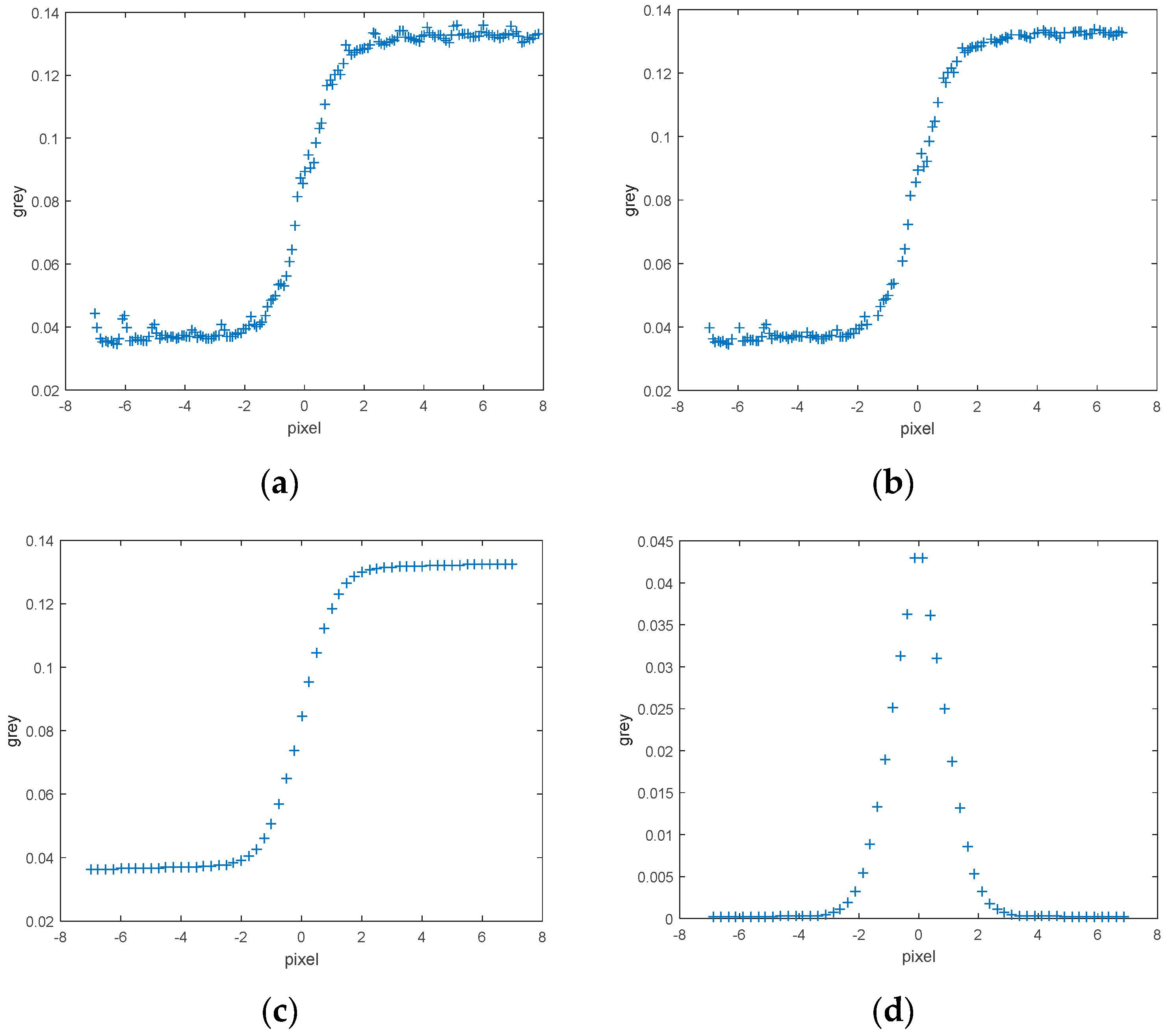
<p>(<b>a</b>) Results of ESF sample; (<b>b</b>) ESF denoised sample; (<b>c</b>) ESF resample; (<b>d</b>) LSF sample.</p> "> Figure 10
<p>Simulation results. (<b>a</b>) Original image; (<b>b</b>) four simulated LR images; (<b>c</b>) one of the LR interpolated images, with the same size as that of the original image.</p> "> Figure 11
<p>Simulation results of experiments with the three methods. The images enclosed in red box are the details of the three different algorithms. (<b>a</b>) Original image; (<b>b</b>) image based on the proposed algorithm; (<b>c</b>) image based on the blind SR reconstruction algorithm; and (<b>d</b>) image based on the bicubic interpolation algorithm.</p> "> Figure 11 Cont.
<p>Simulation results of experiments with the three methods. The images enclosed in red box are the details of the three different algorithms. (<b>a</b>) Original image; (<b>b</b>) image based on the proposed algorithm; (<b>c</b>) image based on the blind SR reconstruction algorithm; and (<b>d</b>) image based on the bicubic interpolation algorithm.</p> "> Figure 12
<p>(<b>a</b>,<b>b</b>) are the experimental data; (<b>c</b>) detail of the road; (<b>d</b>) detail of the house; (<b>e</b>) detail of the paddy fields.</p> "> Figure 13
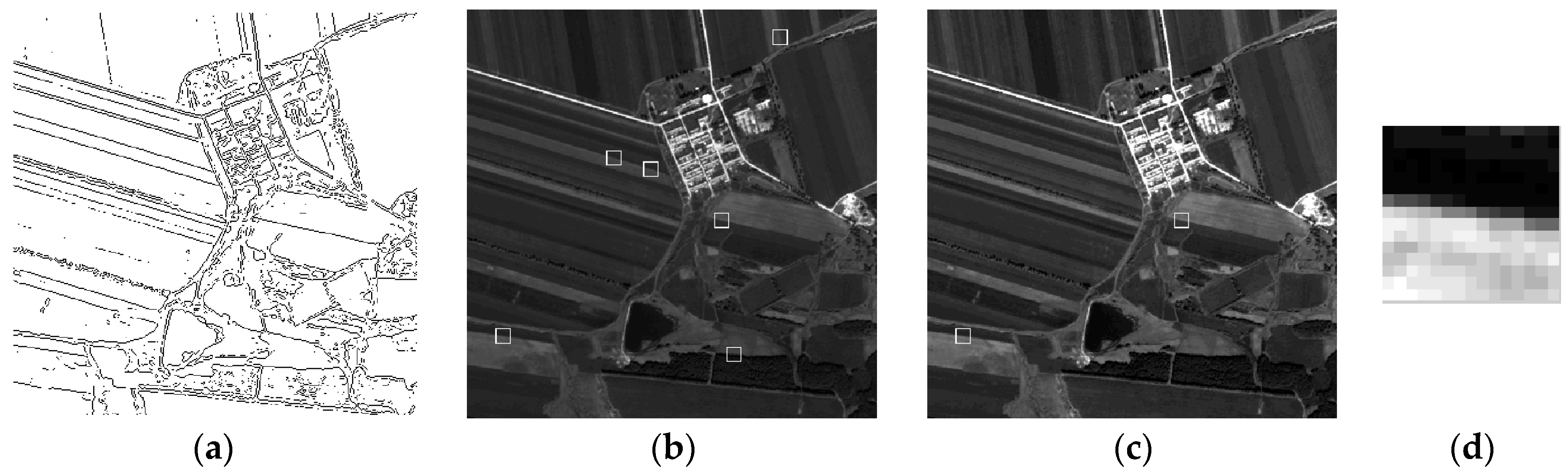
<p>Process of extracting the edge region by using the novel slant knife-edge method. (<b>a</b>) Edge detection by canny algorithm; (<b>b</b>) all knife-edge areas are described in white boxes; (<b>c</b>) preferred knife-edge areas; (<b>d</b>) selected knife-edge area.</p> "> Figure 14
<p>Actual results of the experiments using the three methods. The images enclosed in a red box are the details of the three different algorithms. (<b>a</b>) Original LR image; (<b>b</b>) image based on the proposed algorithm; (<b>c</b>) image based on the blind SR reconstruction algorithm; (<b>d</b>) image based on the bicubic interpolation algorithm; (<b>e</b>) is the detail of reconstruction in region A by the proposed algorithm; (<b>f</b>) is the detail of reconstruction in region A by the blind SR reconstruction algorithm; and (<b>g</b>) is the detail of reconstruction in region A by the bicubic interpolation algorithm.</p> "> Figure 15
<p>Actual results of the second set of experiments using the three methods. The images enclosed in a red box are the details of the three different algorithms. (<b>a</b>) Original LR image; (<b>b</b>) image based on the proposed algorithm; (<b>c</b>) image based on the blind SR reconstruction algorithm; (<b>d</b>) image based on the bicubic interpolation algorithm; (<b>e</b>) is the detail of reconstruction in region A by the proposed algorithm; (<b>f</b>) is the detail of reconstruction in region A by the blind SR reconstruction algorithm; (<b>g</b>) is the detail of reconstruction in region A by the bicubic interpolation algorithm; (<b>h</b>) is the detail of reconstruction in region B by the proposed algorithm; (<b>i</b>) is the detail of reconstruction in region B by the blind SR reconstruction algorithm; and (<b>j</b>) is the detail of reconstruction in region B by the bicubic interpolation algorithm.</p> ">
Abstract
:1. Introduction
2. Materials and Methods
2.1. Observation Model
2.2. Principle of POCS SR Algorithm
- Step 1:
- Estimate the image by using the linear interpolation method for LR images.
- Step 2:
- Compute the motion compensation of the pixel of each LR image. The correspondence between the LR image and the HR image is given by Equation (3):where ( is the point in the LR image, and is the corresponding point in the HR image.
- Obtain the position of the pixel on the LR image of each frame and on the HR image .
- Calculate the parameter, , which represents the range and the value of PSF according to the position of the pixel.
- Simulate the sampling process to obtain the simulated LR image. The observed LR image can be constrained by a convex set , as follows:The projection at any point on is defined in Equation (5) as follows:
- Calculate the residuals between the real image and the simulated image. The formula can be described by (6).where is the impulse response coefficient, is the confidence level on the observed result. In this paper, , where the point is the standard deviation of the noise, and is determined by an appropriate statistical confidence range. These settings define HR images that are consistent with the observed LR image frames within a certain confidence range proportional to the observed noise variation.
- Correct the pixel value of the HR image according to the residuals.
- Step 3:
- Repeat from Step 2 until convergence
2.3. Relationship between and
2.4. PSF Estimation of Low-Resolution Remote Sensing Images
- The area cannot be extracted from the borders of the image to avoid the noise around the borders.
- The area must be excellent in linearity to ensure the accuracy of the PSF estimation.
- Evident gray value differences between two sides of the edge to reduce the influence of the noise must be obtained.
3. Results and Discussion
3.1. Examples of Simulated Images
- The experimental image with some knife-edge areas can be selected by the ADS 40 remote sensing image with the size of 314 × 314, as shown in Figure 10a.
- to the SR observation model, the original blurred image with given low pass and downsampled with factor 2 generated four LR images with the size of 157 × 157, as shown in Figure 10b. One of the LR simulated images is shown in Figure 10c. These four images correspond to the actual transformation parameters of the reference image, as shown in Table 3, where Dx represents the actual offset in the horizontal direction of the simulated LR image, and Dy is the actual offset in the vertical direction. D is the rotation angle because this experiment mainly considered translation; hence, the rotation angle is 0. The default units are pixels and degrees.
- The knife-edge areas with four LR images are estimated using the PSF estimation based on slant knife-edge method, which is an accurate method. PSFs can then be obtained separately.
- According to the derived formula (20), the PSF must be multiplied by the downsampling factor 2. Afterward, the POCS method with the estimated 2*PSF is used to reconstruct the HR image from these four downsampling LR images.
- The blind SR and bicubic interpolation methods are used for the comparative experiments. The similarity between the experimental image and the resulting images of the three methods are observed.
- Evaluation of experimental results.
3.2. Examples of Real Images
4. Conclusions
Acknowledgments
Author Contributions
Conflicts of Interest
References
- Lu, Z.W.; Wu, C.D.; Chen, D.; Qi, Y.; Wei, C. Overview on image super resolution reconstruction. In Proceedings of the 26th Chinese Control and Decision Conference (2014 CCDC), Changsha, China, 31 May–2 June 2014; IEEE: New York, NY, USA, 2014; pp. 2009–2014. [Google Scholar]
- Park, S.C.; Park, M.K.; Kang, M.G. Super-Resolution Image Reconstruction: A Technical Overview. IEEE Trans. Signal Process. Mag. 2003, 20, 21–36. [Google Scholar] [CrossRef]
- Kasturiwala, S.B.; Siddharth, A. Adaptive Image Superresolution for Agrobased Application. In Proceedings of the 2015 International Conference on Industrial Instrumentation and Control (ICIC) of Engineering Pune, Pune, India, 28–30 May 2015; pp. 650–655.
- Ling, F.; Foody, G.M.; Ge, Y.; Li, X.; Du, Y. An Iterative Interpolation Deconvolution Algorithm for Superresolution Land Cover Mapping. IEEE Trans. Geosci. Remote Sens. 2016, 54, 7210–7222. [Google Scholar] [CrossRef]
- Duveiller, G.; Defourny, P.; Gerard, B. A Method to Determine the Appropriate Spatial Resolution Required for Monitoring Crop Growth in a given Agricultural Landscape. In Proceedings of the IEEE International Geoscience and Remote Sensing Symposium, Boston, MA, USA, 7–11 July 2008; pp. 562–565.
- Harris, J.L. Diffraction and resolving power. JOSA 1964, 54, 931–936. [Google Scholar] [CrossRef]
- Goodman, J.W. Introduction to Fourier Optics; Roberts and Company Publishers: New York, NY, USA, 2005. [Google Scholar]
- Sen, P.; Darabi, S. Compressive Image Super-resolution. In Proceedings of the 2009 Conference Record of the Forty-Third Asilomar Conference on Signals, Systems and Computers, Pacific Grove, CA, USA, 1–4 November 2009.
- Hardie, R.C.; Barnard, K.J.; Armstrong, E.E. Armstrong, Joint MAP Registration and High-Resolution Image Estimation Using a Sequence of Undersampled Images. IEEE Trans. Image Process. 1997, 6, 1621–1632. [Google Scholar] [CrossRef] [PubMed]
- Wheeler, F.W.; Liu, X.; Tu, P.H. Multi-frame super-resolution for face recognition. In Proceedings of the First IEEE International Conference on Biometrics: Theory, Applications, and Systems, BTAS 2007, Crystal City, VA, USA, 27–29 September 2007; IEEE: New York, NY, USA, 2007; pp. 1–6. [Google Scholar]
- Irani, M.; Peleg, S. Image sequence enhancement using multiple motions analysis. In Proceedings of the 1992 IEEE Computer Society Conference on Computer Vision and Pattern Recognition, Champaign, IL, USA, 15–18 June 1992; pp. 216–221.
- Irani, M.; Peleg, S. Super resolution from image sequences. In Proceedings of the 10th International Conference on Pattern Recognition, Atlantic City, NJ, USA, 16–21 June 1990; 1990; Volume 2, pp. 115–120. [Google Scholar]
- Stark, H.; Oskoui, P. High resolution image recovery from image plane arrays using convex projections. J. Opt. Soc. Am. 1989, 6, 1715–1726. [Google Scholar] [CrossRef]
- Alam, M.; Jamil, K. Maximum likelihood (ML) based localization algorithm for multi-static passive radar using range-only measurements. In Proceedings of the 2015 IEEE Radar Conference, Sandton, Johannesburg, South Africa, 27–30 October 2015; IEEE: New York, NY, USA, 2015; pp. 180–184. [Google Scholar]
- Hardie, R.C.; Barnard, K.J.; Armstrong, E.E. Joint MAP registration and high-resolution image estimation using a sequence of undersampled images. IEEE Trans. Image Process. 1997, 6, 1621–1633. [Google Scholar] [CrossRef] [PubMed]
- Tom, B.C.; Katsaggelos, A.K. Reconstruction of a high-resolution image by simultaneous registration, restoration, and interpolation of low-resolution images. In Proceedings of the 2nd IEEE Conference on Image Processing, Los Alamitos, CA, USA, 23–26 October 1995; pp. 539–542.
- Elad, M.; Feuer, A. Restoration of a single superresolution image from several blurred, noisy, and undersampled measured images. IEEE Trans. Image Process. 1997, 6, 1646–1658. [Google Scholar] [CrossRef] [PubMed]
- Ogawa, T.; Haseyama, M. Missing intensity interpolation using a kernel PCA-based POCS algorithm and its applications. IEEE Trans. Image Process. 2011, 20, 417–432. [Google Scholar] [CrossRef] [PubMed]
- Xi, H.; Xiao, C.; Bian, C. Edge halo reduction for projections onto convex sets super resolution image reconstruction. In Proceedings of the 2012 International Conference on Digital Image Computing Techniques and Applications (DICTA), Fremantle, Australia, 3–5 December 2012; IEEE: New York, NY, USA, 2012; pp. 1–7. [Google Scholar]
- Liang, F.; Xu, Y.; Zhang, M.; Zhang, L. A POCS Algorithm Based on Text Features for the Reconstruction of Document Images at Super-Resolution. Symmetry 2016, 8, 102. [Google Scholar] [CrossRef]
- Cristóbal, G. Multiframe blind deconvolution coupled with frame registration and resolution enhancement. In Blind Image Deconvolution Theory and Applications; CRC press: Boca Raton, FL, USA, 2007; Volume 3, p. 317. [Google Scholar]
- Nakazawa, S.; Iwasaki, A. Blind super-resolution considering a point spread function of a pushbroom sattelite imaging system. In Proceedings of the IEEE International Geoscience and Remote Sensing Symposium-IGARSS, Melbourne, Australia, 21–26 July 2013; pp. 4443–4446.
- Xie, W.; Zhang, F.; Chen, H.; Qin, Q. Blind super-resolution image reconstruction based on POCS model. In Proceedings of the 2009 international conference on measuring technology and mechatronics automation, Washington, DC, USA, 11–12 April 2009; pp. 437–440.
- Schulz, R.R.; Stevenson, R.L. Extraction of high-resolutionframes from video sequences. IEEE Trans. Image Process. 1996, 5, 996–1011. [Google Scholar] [CrossRef] [PubMed]
- Campisi, P.; Egiazarian, K. Blind Image Deconvolution: Theory and Applications; CRC Press: Boca Raton, FL, USA, 2016. [Google Scholar]
- Fan, C. Super-resolution reconstruction of three-line-scanner images. Ph.D. Thesis, Central South University, Changsha, China, 2007. [Google Scholar]
- Ding, Z.H.; Guo, H.M.; Gao, X.M.; Lan, J.H.; Weng, X.Y.; Man, Z.S.; Zhuang, S.L. The blind restoration of Gaussian blurred image. Opt. Instrum. 2011, 33, 334–338. [Google Scholar]
- Capel, D. Image Mosaicing. In Image Mosaicing and Super-Resolution; Springer: London, UK, 2004; pp. 47–79. [Google Scholar]
- Reichenbach, S.E.; Park, S.K.; Narayanswamy, R. Characterizing digital image acquisition devices. Opt. Eng. 1991, 30, 170–177. [Google Scholar] [CrossRef]
- Yang, J.C.; Wang, Z.W.; Lin, Z.; Cohen, S.; Huang, T. Coupled Dictionary Training for Image Super-Resolution. IEEE Trans. Image Process. 2012, 21, 3467–3478. [Google Scholar] [CrossRef] [PubMed]
- Liu, Z.J.; Wang, C.Y.; Luo, C.F. Estimation of CBERS-1 Point Spread Function and image restoration. J. Remote Sens. 2004, 8, 234–238. [Google Scholar]
- Choi, T. IKONOS Satellite on Orbit Modulation Transfer Function (MTF) Measurement Using Edge and Pulse Method; Engineering South Dakota State University: Brookings, SD, USA, 2002; p. 19. [Google Scholar]
- Deshpande, A.M.; Patnaik, S. Singles image motion deblurring: An accurate PSF estimation and ringing reduction. Int. J. Light Electron Opt. 2014, 125, 3612–3618. [Google Scholar] [CrossRef]
- Leger, D.; Duffaut, J.; Robinet, F. MTF measurement using spotlight. In Proceedings of the IGARSS’94, Surface and Atmospheric Remote Sensing: Technologies, Data Analysis and Interpretation, International Geoscience and Remote Sensing Symposium, Pasadena, CA, USA, 8–12 August 1994; IEEE: New York, NY, USA, 1994; Volume 4, pp. 2010–2012. [Google Scholar]
- Fan, C.; Li, G.; Tao, C. Slant edge method for point spread function estimation. Opt. Soc. Am. 2015, 54, 1–5. [Google Scholar] [CrossRef]
- Wang, Q.J.; Xu, Y.J.; Yuan, Q.Q.; Wang, R.B.; Shen, H.F.; Wang, Y. Restoration of CBERS-02B Remote Sensing Image Based on Knife-edge PSF Estimation and Regularization Reconstruction Model. In Proceedings of the 2011 International Conference on Intelligent Computation Technology and Automation (ICICTA), Shenzhen, China, 28–29 March 2011; pp. 687–690.
- Qin, R.; Gong, J.; Fan, C. Multi-frame image super-resolution based on knife-edges. In Proceedings of the IEEE 10th International Conference on Signal Processing Proceedings, Beijing, China, 24–28 October 2010; IEEE: New York, NY, USA, 2010; pp. 972–975. [Google Scholar]
- Qin, R.J.; Gong, J.Y. A robust method of calculating point spread function from knife-edge without angular constraint in remote sensing images. Yaogan Xuebao J. Remote Sens. 2011, 15, 895–907. [Google Scholar]
- Van Ouwerkerk, J.D. Image super-resolution survey. Image Vision Comput. 2006, 24, 1039–1052. [Google Scholar] [CrossRef]
- Zhu, X.; Milanfar, P. Automatic parameter selection for denoising algorithms using a no-reference measure of image content. IEEE Trans. Image Process. 2010, 19, 3116–3132. [Google Scholar] [PubMed]


| k | k = 0.5 | k = 1.5 | k = 2 | k = 2.5 | k = 3 | ||
|---|---|---|---|---|---|---|---|
| σ | |||||||
| ∑ | |||||||
| 0.5 | 0.3154 | 0.8556 | 1.1164 | 1.401 | 1.6878 | ||
| 0.75 | 0.4375 | 1.1739 | 1.5565 | 1.944 | 2.3341 | ||
| 1 | 0.5476 | 1.5337 | 2.0346 | 2.5461 | 3.0514 | ||
| 1.5 | 0.7861 | 2.2715 | 3.0206 | 3.7757 | 4.5295 | ||
| 1.75 | 0.9101 | 2.642 | 3.5195 | 4.3967 | 5.2731 | ||
| 2 | 1.0336 | 3.0144 | 4.0175 | 5.019 | 6.0212 | ||
| 2.5 | 1.2775 | 3.7623 | 5.0135 | 6.2669 | 7.5232 | ||
| Original Image (σ) | Estimate of Downsampling Image (σ/2) | Real Result of Each Downsampling Image | |
|---|---|---|---|
| Example 1 | 0.5894 | 0.2992 | 0.2979 |
| 0.3067 | |||
| 0.3102 | |||
| 0.3098 | |||
| Example 2 | 0.3809 | 0.1905 | 0.2235 |
| 0.2158 | |||
| 0.1884 | |||
| 0.1923 |
| Dx | Dy | Dθ | |
|---|---|---|---|
| 1 | 0.5 | 0.5 | 0 |
| 2 | 1.2 | 1.2 | 0 |
| 3 | 0.4 | 0.4 | 0 |
| 4 | 1.8 | 1.8 | 0 |
| Image | PSNR | MSE |
|---|---|---|
| Image based on the proposed algorithm | 96.7904 | |
| Image based on the blind SR reconstruction algorithm | 54.5366 | |
| Image based on the bicubic interpolation algorithm | 81.8529 |
| Number | [X, Y] | Relevant |
|---|---|---|
| 1 | [36, 320] | 0.9825 |
| 2 | [249, 207] | 0.9763 |
| 3 | [144, 146] | 0.9748 |
| 4 | [180, 157] | 0.9722 |
| 5 | [261, 338] | 0.9557 |
| 6 | [306, 28] | 0.9187 |
| Image Reconstructed by Different Algorithms | The Value of Q |
|---|---|
| the proposed algorithm | 24.2285 |
| the blind SR reconstruction algorithm | 21.6771 |
| the bicubic interpolation algorithm | 17.3591 |
| Image Reconstructed by Different Algorithms | The Value of Q |
|---|---|
| the proposed algorithm | 40.1082 |
| the blind SR reconstruction algorithm | 34.8491 |
| the bicubic interpolation algorithm | 28.3006 |
© 2017 by the authors. Licensee MDPI, Basel, Switzerland. This article is an open access article distributed under the terms and conditions of the Creative Commons Attribution (CC BY) license ( http://creativecommons.org/licenses/by/4.0/).
Share and Cite
Fan, C.; Wu, C.; Li, G.; Ma, J. Projections onto Convex Sets Super-Resolution Reconstruction Based on Point Spread Function Estimation of Low-Resolution Remote Sensing Images. Sensors 2017, 17, 362. https://doi.org/10.3390/s17020362
Fan C, Wu C, Li G, Ma J. Projections onto Convex Sets Super-Resolution Reconstruction Based on Point Spread Function Estimation of Low-Resolution Remote Sensing Images. Sensors. 2017; 17(2):362. https://doi.org/10.3390/s17020362
Chicago/Turabian StyleFan, Chong, Chaoyun Wu, Grand Li, and Jun Ma. 2017. "Projections onto Convex Sets Super-Resolution Reconstruction Based on Point Spread Function Estimation of Low-Resolution Remote Sensing Images" Sensors 17, no. 2: 362. https://doi.org/10.3390/s17020362