Unravelling the Relationship Between Microseisms and Spatial Distribution of Sea Wave Height by Statistical and Machine Learning Approaches

 ,
,  , , , ,
 "> Figure 1
<p>Map of a portion of the Mediterranean Sea, showing bathymetry (data from <a href="http://marine.copernicus.eu/" target="_blank">http://marine.copernicus.eu/</a>) and the location of the six seismic stations used in this work (black dots and labels). The inset in the right upper corner shows the digital elevation model of Eastern Sicily, with the location of the seismic stations.</p> "> Figure 2
<p>(<b>a</b>–<b>f</b>) Spectrograms of the seismic signal recorded by the vertical component of the six considered stations. (<b>g</b>–<b>l</b>) Median spectra of the seismic signal recorded by the vertical component of the six considered stations. Arrows and labels in (<b>g</b>–<b>l</b>) indicate the spectral peaks corresponding to short-period secondary microseisms (SPSM), secondary microseisms (SM) and primary microseisms (PM).</p> "> Figure 3
<p>RMS amplitudes of the seismic signal recorded by the vertical component of the six considered stations (<b>a</b>: AIO; <b>b</b>: EFIU; <b>c</b>: EPOZ; <b>d</b>: HAGA; <b>e</b>: HLNI; <b>f</b>: MSRU), and filtered in the band 0.05–0.4 Hz, comprising short-period secondary, secondary, and primary microseisms.</p> "> Figure 4
<p>Maps of a portion of the Mediterranean Sea, showing the spatial distribution of Spearman’s correlation coefficient computed between significant sea wave height and seismic RMS amplitudes, calculated on the vertical component of the six considered stations and filtered in different frequency bands (see plot titles). The black dots indicate the locations of the considered stations.</p> "> Figure 5
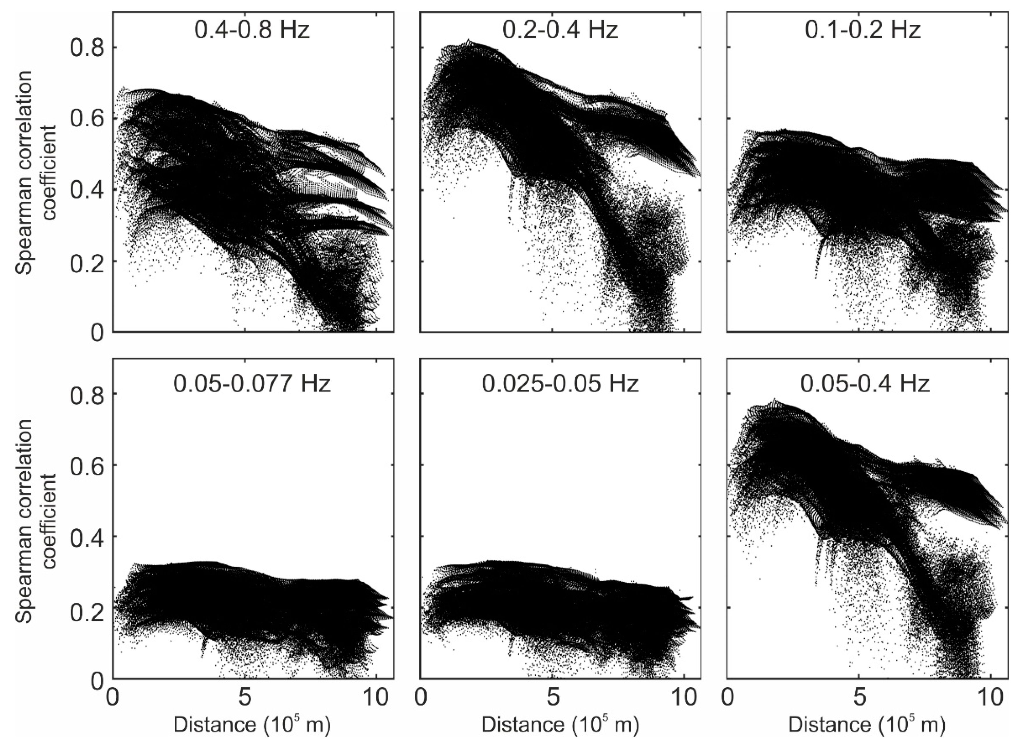
<p>Cross-plots showing the relationship between Spearman’s correlation coefficient, computed between significant sea wave height and seismic RMS amplitudes at different frequency bands (see plot titles), and the distance between the seismic station and the sea grid cell.</p> "> Figure 6
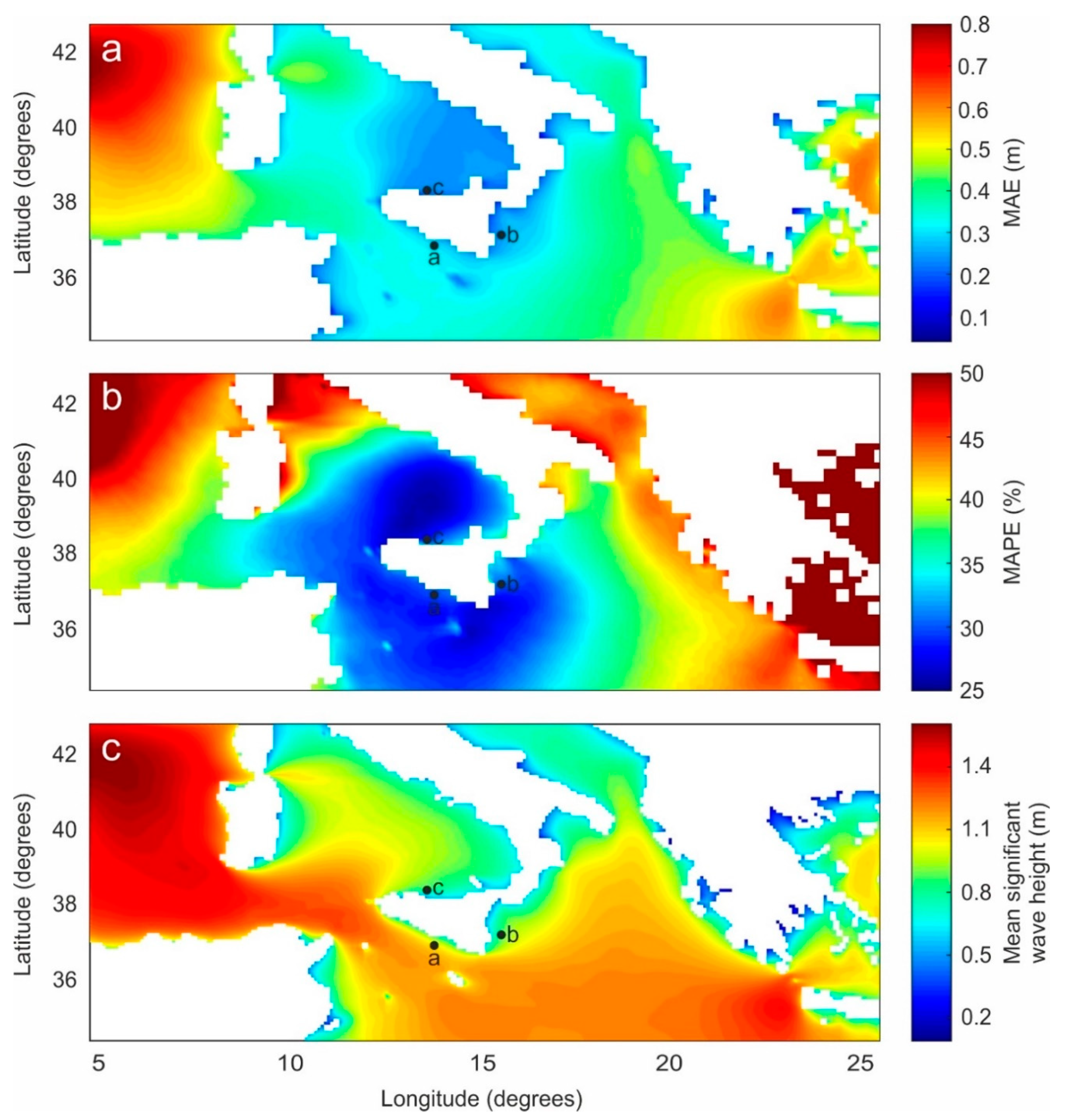
<p>Spatial distribution of (<b>a</b>) mean absolute error (MAE), (<b>b</b>) mean absolute percentage error (MAPE), and (<b>c</b>) mean significant wave height computed during the interval 2010–2017. The black dots with labels “a,” “b,” and “c” indicate the locations of the grid cells, which the cross-plots in <a href="#remotesensing-12-00761-f007" class="html-fig">Figure 7</a> are referred to.</p> "> Figure 7
<p>Scatter plots showing the hindcast significant wave height versus the predicted significant wave height from January 2010 to October 2017 for three grid cells, whose locations are indicated in <a href="#remotesensing-12-00761-f006" class="html-fig">Figure 6</a>. The red dashed line in (<b>a</b>–<b>c</b>) is the y = x line. The value of the determination coefficient (R<sup>2</sup>) is also reported in the plots.</p> "> Figure 8
<p>(<b>a</b>–<b>c</b>) Hindcast maps of significant sea wave height, (<b>d</b>–<b>f</b>) predicted maps of significant sea wave height based on microseism data, and (<b>g</b>–<b>i</b>) corresponding spatial distribution of the prediction error, computed as the difference between the predicted maps and the hindcast maps, during three selected time intervals: (a,d,g) 03/11/2017 01:00, (b,e,h) 28/12/2017 17:00, and (c,f,i) 29/12/2017 05:00.</p> "> Figure 9
<p>(<b>a</b>–<b>c</b>) Index of importance of all the inputs taken into account for the three grid cells labelled “a,” “b,” and “c” in <a href="#remotesensing-12-00761-f006" class="html-fig">Figure 6</a>, respectively. (<b>d</b>–<b>f</b>) Aggregation through summation of the input importance allowing the ranking of the frequency bands for three grid cells labelled “a,” “b,” and “c” in <a href="#remotesensing-12-00761-f006" class="html-fig">Figure 6</a>, respectively. (<b>g</b>–<b>i</b>) Aggregation through summation of the input importance allowing the ranking of seismic stations for three grid cells labelled “a,” “b,” and “c” in <a href="#remotesensing-12-00761-f006" class="html-fig">Figure 6</a>, respectively.</p> ">
Abstract
:
1. Introduction
2. Materials and Methods
2.1. Data
2.2. Spectral and Amplitude Analysis
2.3. Correlation Analysis
2.4. Machine Learning
- Dividing the original input dataset into two complementary subsets;
- building a model on one subset (called the “training set”) (step a);
- validating the model performance on the other subset (“validation set”) (step b);
- repeating (i–iii) “k” times, selecting different time intervals as the training set and validation set each time.
3. Results
4. Discussion
5. Conclusions
- Short-period secondary microseisms showed the highest amplitude values among the considered frequency bands. In addition, high seismic amplitudes were observed at frequencies above the short-period secondary microseism band (0.4–0.8 Hz), likely related to energy transfer from the hydrosphere/atmosphere to the solid earth.
- Seasonal modulations of microseism amplitudes, due to the more efficient energy transfer from the sea to the solid earth in winters, when the seas are stormier, were identified.
- Correlation analysis suggests how the microseism recorded by the considered stations is mostly generated by sources located close to the stations, and then to the Eastern Sicilian coastlines.
- Machine learning analysis shows promising results in the spatial reconstruction of sea state in terms of significant wave height by microseism data. In the future, a reliable reconstruction of the sea state in wide areas will need microseism data recorded by dense networks, comprising stations evenly distributed along the coastlines.
Author Contributions
Funding
Acknowledgments
Conflicts of Interest
Data Availability
References
- Von Storch, H.; Emeis, K.; Meinke, I.; Kannen, A.; Matthias, V.; Ratter, B.M.; Stanev, E.; Weisse, R.; Wirtz, K. Making coastal research useful – cases from practice. Oceanol. 2015, 57, 3–16. [Google Scholar] [CrossRef] [Green Version]
- Ferretti, G.; Barani, S.; Scafidi, D.; Capello, M.; Cutroneo, L.; Vagge, G.; Besio, G. Near real-time monitoring of significant sea wave height through microseism recordings: An application in the Ligurian Sea (Italy). Ocean Coast. Manag. 2018, 165, 185–194. [Google Scholar] [CrossRef]
- Reguero, B.G.; Losada, I.J.; Méndez, F.J. A recent increase in global wave power as a consequence of oceanic warming. Nat. Commun. 2019, 10, 205. [Google Scholar] [CrossRef] [PubMed] [Green Version]
- Holthuijsen, L.H. Waves in Oceanic and Coastal Waters; Cambridge University Press: Cambridge, UK, 2007. [Google Scholar]
- Orasi, A.; Picone, M.; Drago, A.; Capodici, F.; Gauci, A.; Nardone, G.; Inghilesi, R.; Azzopardi, J.; Galea, A.; Ciraolo, G.; et al. HF radar for wind waves measurements in the Malta-Sicily Channel. Measurement 2018, 128, 446–454. [Google Scholar] [CrossRef]
- Fu, L.-L.; Cazenave, A. Satellite Altimetry and Earth Sciences: A Handbook of Techniques and Applications, Satell; Elsevier: Amsterdam, The Netherlands, 2000. [Google Scholar]
- Wiese, A.; Staneva, J.; Schultz-Stellenfleth, J.; Behrens, A.; Fenoglio-Marc, L.; Bidlot, J.-R. Synergy between satellite observations and model simulations during extreme events. Ocean Sci. Discuss. 2018, 14, 1503–1521. [Google Scholar] [CrossRef] [Green Version]
- Musa, Z.; Popescu, I.; Mynett, A. A review of applications of satellite SAR, optical, altimetry and DEM data for surface water modelling, mapping and parameter estimation. Hydrol. Earth Syst. Sci. 2015, 19, 3755–3769. [Google Scholar] [CrossRef] [Green Version]
- Wyatt, L.R.; Green, J.J. Measuring high and low waves with HF radar. OCEANS 2009-EUROPE 2009, 1–5. [Google Scholar]
- Wyatt, L.R.; Green, J.J.; Middleditch, A. Signal Sampling Impacts on HF Radar Wave Measurement. J. Atmos. Ocean. Technol. 2009, 26, 793–805. [Google Scholar] [CrossRef]
- Zopf, D.O.; Creech, H.C.; Quinn, W.H. Wavemeter: A Land-Based System for Measuring Nearshore Ocean Waves. Mar. Technol. Soc. J. 1976, 10, 19–25. [Google Scholar]
- Bromirski, P.D.; Duennebier, F.K. The near-coastal microseism spectrum: Spatial and temporal wave climate relationships. J. Geophys. Res. Space Phys. 2002, 107, 1–20. [Google Scholar] [CrossRef] [Green Version]
- Anthony, R.E.; Aster, R.C.; McGrath, D. Links between atmosphere, ocean, and cryosphere from two decades of microseism observations on the Antarctic Peninsula. J. Geophys. Res. Earth Surf. 2017, 122, 153–166. [Google Scholar] [CrossRef]
- Hasselmann, K. A statistical analysis of the generation of microseisms. Rev. Geophys. 1963, 1, 177. [Google Scholar] [CrossRef]
- Longuet-Higgins, M.S. A theory of the origin of microseisms. Philos. Trans. R. Soc. London. Ser. A, Math. Phys. Sci. 1950, 243, 1–35. [Google Scholar]
- Oliver, J.; Page, R. Concurrent Storms of Long and Ultralong Period Microseisms. Bull. Seism. Soc. Am. 1963, 53, 15–26. [Google Scholar]
- Bromirski, P.D.; Duennebier, F.K.; Stephen, R. Mid-ocean microseisms. Geochem. Geophys. Geosyst. 2005, 6, 6. [Google Scholar] [CrossRef]
- Chen, Y.-N.; Gung, Y.; You, S.-H.; Hung, S.-H.; Chiao, L.-Y.; Huang, T.-Y.; Chen, Y.-L.; Liang, W.-T.; Jan, S. Characteristics of short period secondary microseisms (SPSM) in Taiwan: The influence of shallow ocean strait on SPSM. Geophys. Res. Lett. 2011, 38, 1–5. [Google Scholar] [CrossRef] [Green Version]
- Cannata, A.; Cannavo’, F.; Moschella, S.; Gresta, S.; Spina, L. Exploring the link between microseism and sea ice in Antarctica by using machine learning. Sci. Rep. 2019, 9, 13050. [Google Scholar] [CrossRef]
- Bromirski, P.D.; Flick, R.E.; Graham, N. Ocean wave height determined from inland seismometer data: Implications for investigating wave climate changes in the NE Pacific. J. Geophys. Res. Space Phys. 1999, 104, 20753–20766. [Google Scholar] [CrossRef]
- Ardhuin, F.; Stutzmann, E.; Schimmel, M.; Mangeney, A. Ocean wave sources of seismic noise. J. Geophys. Res. Space Phys. 2011, 116, 1–21. [Google Scholar] [CrossRef]
- Ferretti, G.; Zunino, A.; Scafidi, D.; Barani, S.; Spallarossa, D. On microseisms recorded near the Ligurian coast (Italy) and their relationship with sea wave height. Geophys. J. Int. 2013, 194, 524–533. [Google Scholar] [CrossRef] [Green Version]
- Ferretti, G.; Scafidi, D.; Cutroneo, L.; Gallino, S.; Capello, M. Applicability of an empirical law to predict significant sea-wave heights from microseisms along the Western Ligurian Coast (Italy). Cont. Shelf Res. 2016, 122, 36–42. [Google Scholar] [CrossRef]
- Behrens, A. Documentation of a Web Based Source Code Library for WAM. 2013. Available online: https://github.com/mywave/WAM/tree/master/documentation (accessed on 24 February 2020).
- Welch, P. The use of fast Fourier transform for the estimation of power spectra: A method based on time averaging over short, modified periodograms. IEEE Trans. Audio Electroacoustics 1967, 15, 70–73. [Google Scholar] [CrossRef] [Green Version]
- Bromirski, P.D. Vibrations from the “Perfect Storm”. Geochem. Geophys. Geosyst. 2001, 2, 2. [Google Scholar] [CrossRef]
- Essen, H.-H.; Krüger, F.; Dahm, T.; Grevemeyer, I. On the generation of secondary microseisms observed in northern and central Europe. J. Geophys. Res. Space Phys. 2003, 108, 1–15. [Google Scholar] [CrossRef]
- Craig, D.; Bean, C.; Lokmer, I.; Möllhoff, M. Correlation of Wavefield-Separated Ocean-Generated Microseisms with North Atlantic Source Regions. Bull. Seism. Soc. Am. 2016, 106, 1002–1010. [Google Scholar] [CrossRef]
- Xiao, H.; Xue, M.; Yang, T.; Liu, C.; Hua, Q.; Xia, S.; Huang, H.; Le, B.M.; Yu, Y.; Huo, D.; et al. The Characteristics of Microseisms in South China Sea: Results From a Combined Data Set of OBSs, Broadband Land Seismic Stations, and a Global Wave Height Model. J. Geophys. Res. Solid Earth 2018, 123, 3923–3942. [Google Scholar] [CrossRef]
- Breiman, L. Random forests. Mach. Learn. 2001, 45, 5–32. [Google Scholar] [CrossRef] [Green Version]
- Kuhn, M.; Johnson, K. Applied Predictive Modeling; Springer: New York, NY, USA, 2013; ISBN 9781461468493. [Google Scholar]
- Carranza, E.J.M.; Laborte, A.G. Random forest predictive modeling of mineral prospectivity with small number of prospects and data with missing values in Abra (Philippines). Comput. Geosci. 2015, 74, 60–70. [Google Scholar] [CrossRef]
- Kuhn, S.; Cracknell, M.; Reading, A.M. Lithologic mapping using Random Forests applied to geophysical and remote-sensing data: A demonstration study from the Eastern Goldfields of Australia. Geophys. 2018, 83, B183–B193. [Google Scholar] [CrossRef]
- Keller, C.A.; Evans, M. Application of random forest regression to the calculation of gas-phase chemistry within the GEOS-Chem chemistry model v10. Geosci. Model Dev. 2019, 12, 1209–1225. [Google Scholar] [CrossRef] [Green Version]
- Lange, N.; Bishop, C.M.; Ripley, B.D. Neural Networks for Pattern Recognition. J. Am. Stat. Assoc. 1997, 92, 1642. [Google Scholar] [CrossRef]
- Aster, R.C.; McNamara, D.E.; Bromirski, P.D. Global trends in extremal microseism intensity. Geophys. Res. Lett. 2010, 37, 1–5. [Google Scholar] [CrossRef] [Green Version]
- Gal, M.; Reading, A.M.; Ellingsen, S.; Gualtieri, L.; Koper, K.D.; Burlacu, R.; Tkalčić, H.; Hemer, M. The frequency dependence and locations of short-period microseisms generated in the Southern Ocean and West Pacific. J. Geophys. Res. Solid Earth 2015, 120, 5764–5781. [Google Scholar] [CrossRef]
- Möllhoff, M.; Bean, C. Seismic Noise Characterization in Proximity to Strong Microseism Sources in the Northeast Atlantic. Bull. Seism. Soc. Am. 2016, 106, 464–477. [Google Scholar] [CrossRef]
- Cannata, A.; Di Grazia, G.; Montalto, P.; Ferrari, F.; Nunnari, G.; Patane’, D.; Privitera, E. New insights into banded tremor from the 2008–2009 Mount Etna eruption. J. Geophys. Res. Space Phys. 2010, 115, 1–22. [Google Scholar] [CrossRef]
- Aster, R.C.; McNamara, D.E.; Bromirski, P.D. Multidecadal Climate-induced Variability in Microseisms. Seism. Res. Lett. 2008, 79, 194–202. [Google Scholar] [CrossRef]
- Stutzmann, E.; Schimmel, M.; Patau, G.; Maggi, A. Global climate imprint on seismic noise. Geochem. Geophys. Geosyst. 2009, 10, 10. [Google Scholar] [CrossRef]
- Grob, M.; Maggi, A.; Stutzmann, E. Observations of the seasonality of the Antarctic microseismic signal, and its association to sea ice variability. Geophys. Res. Lett. 2011, 38, 38. [Google Scholar] [CrossRef] [Green Version]
- Essen, H.-H.; Klussmann, J.; Herber, R.; Grevemeyer, I. Does microseisms in Hamburg (Germany) reflect the wave climate in the North Atlantic?Spiegelt die in Hamburg gemessene Mikroseismik das Wellenklima im Nordatlantik wider? Dtsch. Hydrogr. Zeitschrift 1999, 51, 33–45. [Google Scholar] [CrossRef]
- Cessaro, R.K. Sources of primary and secondary microseisms. Bull. Seismol. Soc. Am. 1994, 84, 142–148. [Google Scholar]
- Chevrot, S.; Sylvander, M.; Benahmed, S.; Ponsolles, C.; Lefèvre, J.M.; Paradis, D. Source locations of secondary microseisms in western Europe: Evidence for both coastal and pelagic sources. J. Geophys. Res. Solid Earth 2007, 112, 1–19. [Google Scholar]
- Bromirski, P.D.; Stephen, R.; Gerstoft, P. Are deep-ocean-generated surface-wave microseisms observed on land? J. Geophys. Res. Solid Earth 2013, 118, 3610–3629. [Google Scholar] [CrossRef] [Green Version]
- Gualtieri, L.; Stutzmann, E.; Juretzek, C.; Hadziioannou, C.; Ardhuin, F. Global scale analysis and modelling of primary microseisms. Geophys. J. Int. 2019, 218, 560–572. [Google Scholar] [CrossRef]


| Station Name | Longitude | Latitude | Altitude (m a.s.l.) |
|---|---|---|---|
| MSRU | 15.5083 | 38.2638 | 401 |
| AIO | 15.2278 | 37.9689 | 715 |
| EFIU | 15.2101 | 37.7897 | 98 |
| EPOZ | 15.1885 | 37.6718 | 119 |
| HAGA | 15.1552 | 37.2853 | 126 |
| HLNI | 14.872 | 37.3485 | 147 |
© 2020 by the authors. Licensee MDPI, Basel, Switzerland. This article is an open access article distributed under the terms and conditions of the Creative Commons Attribution (CC BY) license (http://creativecommons.org/licenses/by/4.0/).
Share and Cite
Cannata, A.; Cannavò, F.; Moschella, S.; Di Grazia, G.; Nardone, G.; Orasi, A.; Picone, M.; Ferla, M.; Gresta, S. Unravelling the Relationship Between Microseisms and Spatial Distribution of Sea Wave Height by Statistical and Machine Learning Approaches. Remote Sens. 2020, 12, 761. https://doi.org/10.3390/rs12050761
Cannata A, Cannavò F, Moschella S, Di Grazia G, Nardone G, Orasi A, Picone M, Ferla M, Gresta S. Unravelling the Relationship Between Microseisms and Spatial Distribution of Sea Wave Height by Statistical and Machine Learning Approaches. Remote Sensing. 2020; 12(5):761. https://doi.org/10.3390/rs12050761
Chicago/Turabian StyleCannata, Andrea, Flavio Cannavò, Salvatore Moschella, Giuseppe Di Grazia, Gabriele Nardone, Arianna Orasi, Marco Picone, Maurizio Ferla, and Stefano Gresta. 2020. "Unravelling the Relationship Between Microseisms and Spatial Distribution of Sea Wave Height by Statistical and Machine Learning Approaches" Remote Sensing 12, no. 5: 761. https://doi.org/10.3390/rs12050761