Estimating Uncertainty of Point-Cloud Based Single-Tree Segmentation with Ensemble Based Filtering

"> Figure 1
<p>(<b>a</b>) Global and country level context. (<b>b</b>) ALS point cloud (high vegetation only) of the study site represented with a false color composite (Red channel = ALS intensity rescaled to 0–1 range, Green channel = aerial image Red, Blue channel = aerial image Green). For leaf-off ALS acquisitions, this color scheme helps differentiate foliage persistence (red represents persistent foliage and green deciduous foliage). The yellow polygon indicates the extent of the field survey. (<b>c</b>) False color composite oblique view of the ALS point cloud (high vegetation only). (<b>d</b>) Side (first row) and top (second row) view of manually delineated tree examples.</p> "> Figure 2
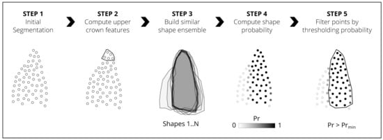
<p>Main steps used to compute shape probability and subsequently filter the initial segment shape.</p> "> Figure 3
<p>(<b>a</b>) Tree top detection results with variable size convolution window. (<b>b</b>) Raster CHM segmentation obtained with the marker controlled watershed algorithm.</p> "> Figure 4
<p>(<b>a</b>) The total height (h), the 3D convex alpha shape (in red) volume (v) and the median intensity (i) of points located in the top 15 % of the tree crown are used as features because they are less affected by poor segmentation. (<b>b</b>) The single region 3D alpha shape (outlined in blue) derived from the point cloud segment.</p> "> Figure 5
<p>Example of an ensemble containing 69 overlaid segments with similar features. Dense point areas indicate high shape probability. (<b>a</b>) Side view (<b>b</b>) Top view.</p> "> Figure 6
<p>Each point cloud segment <math display="inline"> <semantics> <msub> <mi>P</mi> <mn>0</mn> </msub> </semantics> </math> is overlaid with the <math display="inline"> <semantics> <msub> <mi>S</mi> <mrow> <mn>0</mn> <mo>..</mo> <mi>N</mi> </mrow> </msub> </semantics> </math> alpha shapes of similar segments (including itself). Regions of the point cloud segment which occur more frequently inside <math display="inline"> <semantics> <msub> <mi>S</mi> <mrow> <mn>0</mn> <mo>..</mo> <mi>N</mi> </mrow> </msub> </semantics> </math> obtain a higher shape probability. Thus, inconsistencies between the shapes in the ensemble can be detected.</p> "> Figure 7
<p>Individual segment delineation accuracy. The reference shape (in gray) represents the extent of the manually delineated tree. For visualization purposes, the boundaries of the union (in orange) and intersection (in blue) alpha shapes are spatially separated from the points. In reality, the alpha shape boundary passes though the boundary points.</p> "> Figure 8
<p>Sensitivity of the median validation scores to <math display="inline"> <semantics> <mrow> <mi>P</mi> <msub> <mi>r</mi> <mrow> <mi>m</mi> <mi>i</mi> <mi>n</mi> </mrow> </msub> </mrow> </semantics> </math>. Notice that the delineation scores are undefined when the detection rate reaches 0.</p> "> Figure 9
<p>Boxplots of delineation scores before and after filtering the segments with <math display="inline"> <semantics> <mrow> <mi>P</mi> <msub> <mi>r</mi> <mrow> <mi>m</mi> <mi>i</mi> <mi>n</mi> </mrow> </msub> <mo>=</mo> <mn>0.25</mn> </mrow> </semantics> </math>. All the delineation scores except recall are significantly higher after filtering. It can also be noted that the filtering reduces the score spread.</p> "> Figure 10
<p>(<b>a</b>) Shape probability map (high vegetation only). (<b>b</b>) Side (first row) and top (second row) view of shape probability for six example segments. Notice that segment n°3 has null probability. This is explained by the fact it is a particularly high tree and there was an insufficient number of similar trees to form a reliable ensemble. (<b>c</b>) Filtered segments using <math display="inline"> <semantics> <mrow> <mi>P</mi> <msub> <mi>r</mi> <mrow> <mi>m</mi> <mi>i</mi> <mi>n</mi> </mrow> </msub> <mo>=</mo> <mn>0.25</mn> </mrow> </semantics> </math>.</p> ">
Abstract
:
1. Introduction
- Tree top geometric features can be used as proxies of overall tree shape.
- Tree crowns exhibit approximate radial symmetry.
- Tree growth is approximately vertical.
2. Materials
- is the normalized intensity;
- I is the raw intensity;
- r is the range between the sensor and the point;
- is an arbitrary constant reference range (1000 m was used here).
- Most of the tree shape variability for the species (spruce and fir here) and heights of interest should be covered.
- It is expected that the reliability of the average shape estimation increases with the number of observations. So, multiple examples of the same tree shape should be available to ensure an ensemble size that allows determination of the average shape unambiguously.
- If radiometric features are used to build the ensembles, all sample areas should be in the same phenological stage and echo intensity must be rescaled to a common range.
3. Methods
3.1. Overview
3.2. Step 1-Initial Segmentation
3.3. Step 2-Computing Upper Crown Features
3.4. Step 3-Building Shape Ensembles (Grouping Similar Segments)
- N is the number of points in segment i;
- is a N × 3 matrix containing the normalized 3D point coordinates of segment i;
- is a N × 3 matrix containing the original 3D point coordinates of segment i;
- is a 1 × 3 matrix containing the root coordinate of the segment i (i.e., the projection of the tree top on the terrain model);
- is a N × 1 vector of ones.
3.5. Step 4-Computing Shape Probability
- is the alpha shape of segment i;
- is the set of N alpha shapes with features similar to ;
- N is the number of segments in the ensemble i;
- is the minimum number of segments per ensemble required to compute a reliable shape probability (10 was used here).
3.6. Step 5-Filtering
- is the indicator function which produces the filtered point subset;
- is the shape probability associated with each point in segment i;
- is the minimum probability required to retain a point in the segment.
4. Results
4.1. Validation Metrics
4.2. Performance
5. Discussion
6. Conclusions
Acknowledgments
Author Contributions
Conflicts of Interest
Abbreviations
| ALS | Airborne Laser Scanning |
| CHM | Canopy Height Model |
| DBH | Diameter at Breast Height |
| FN | False Negative |
| FP | False Positive |
| GNSS | Global Navigation Satellite System |
| IoU | Intersection over Union |
| ITC | Individual Tree Crown |
| RGB | Red-Green-Blue |
| TIN | Triangular Irregular Network |
| TP | True Positive |
References
- Maltamo, M.; Næsset, E.; Vauhkonen, J. (Eds.) Forestry Applications of Airborne Laser Scanning. In Managing Forest Ecosystems; Springer: Dordrecht, The Netherlands, 2014; Volume 27. [Google Scholar]
- Waser, L.T.; Boesch, R.; Wang, Z.; Ginzler, C. Towards Automated Forest Mapping. In Mapping Forest Landscape Patterns; Springer: New York, NY, USA, 2017; pp. 263–304. [Google Scholar]
- Wulder, M.A.; White, J.C.; Nelson, R.F.; Næsset, E.; Ørka, H.O.; Coops, N.C.; Hilker, T.; Bater, C.W.; Gobakken, T. Lidar Sampling for Large-Area Forest Characterization: A Review. Remote Sens. Environ. 2012, 121, 196–209. [Google Scholar] [CrossRef]
- Wang, Y.; Hyyppä, J.; Liang, X.; Kaartinen, H.; Yu, X.; Lindberg, E.; Holmgren, J.; Qin, Y.; Mallet, C.; Ferraz, A.; et al. International Benchmarking of the Individual Tree Detection Methods for Modeling 3-D Canopy Structure for Silviculture and Forest Ecology Using Airborne Laser Scanning. IEEE Trans. Geosci. Remote Sens. 2016, 54, 5011–5027. [Google Scholar] [CrossRef]
- Zhen, Z.; Quackenbush, L.J.; Zhang, L. Trends in Automatic Individual Tree Crown Detection and Delineation—Evolution of LiDAR Data. Remote Sens. 2016, 8, 333. [Google Scholar] [CrossRef]
- Eysn, L.; Hollaus, M.; Lindberg, E.; Berger, F.; Monnet, J.M.; Dalponte, M.; Kobal, M.; Pellegrini, M.; Lingua, E.; Mongus, D.; Pfeifer, N. A Benchmark of Lidar-Based Single Tree Detection Methods Using Heterogeneous Forest Data from the Alpine Space. Forests 2015, 6, 1721–1747. [Google Scholar] [CrossRef] [Green Version]
- Vauhkonen, J.; Ene, L.; Gupta, S.; Heinzel, J.; Holmgren, J.; Pitkänen, J.; Solberg, S.; Wang, Y.; Weinacker, H.; Hauglin, K.M.; et al. Comparative Testing of Single-Tree Detection Algorithms under Different Types of Forest. For. Int. J. For. Res. 2012, 85, 27–40. [Google Scholar] [CrossRef]
- Kaartinen, H.; Hyyppä, J.; Yu, X.; Vastaranta, M.; Hyyppä, H.; Kukko, A.; Holopainen, M.; Heipke, C.; Hirschmugl, M.; Morsdorf, F.; et al. An International Comparison of Individual Tree Detection and Extraction Using Airborne Laser Scanning. Remote Sens. 2012, 4, 950–974. [Google Scholar] [CrossRef] [Green Version]
- Yin, D.; Wang, L. How to Assess the Accuracy of the Individual Tree-Based Forest Inventory Derived from Remotely Sensed Data: A Review. Int. J. Remote Sens. 2016, 37, 4521–4553. [Google Scholar] [CrossRef]
- Swetnam, T.L.; Falk, D.A. Application of Metabolic Scaling Theory to Reduce Error in Local Maxima Tree Segmentation from Aerial LiDAR. For. Ecol. Manag. 2014, 323, 158–167. [Google Scholar] [CrossRef]
- Sačkov, I.; Hlásny, T.; Bucha, T.; Juriš, M. Integration of Tree Allometry Rules to Treetops Detection and Tree Crowns Delineation Using Airborne Lidar Data. iFor. Biogeosci. For. 2017, 10, 459. [Google Scholar] [CrossRef]
- Pouliot, D.; King, D. Approaches for Optimal Automated Individual Tree Crown Detection in Regenerating Coniferous Forests. Can. J. Remote Sens. 2005, 31, 255–267. [Google Scholar] [CrossRef]
- Heinzel, J.N.; Weinacker, H.; Koch, B. Prior-Knowledge-Based Single-Tree Extraction. Int. J. Remote Sens. 2011, 32, 4999–5020. [Google Scholar] [CrossRef]
- Ene, L.; Næsset, E.; Gobakken, T. Single Tree Detection in Heterogeneous Boreal Forests Using Airborne Laser Scanning and Area-Based Stem Number Estimates. Int. J. Remote Sens. 2012, 33, 5171–5193. [Google Scholar] [CrossRef]
- Pirotti, F. Assessing a Template Matching Approach for Tree Height and Position Extraction from Lidar-Derived Canopy Height Models of Pinus Pinaster Stands. Forests 2010, 1, 194–208. [Google Scholar]
- Holmgren, J.; Lindberg, E. Tree Crown Segmentation Based on a Geometric Tree Crown Model for Prediction of Forest Variables. Can. J. Remote Sens. 2013, 39, S86–S98. [Google Scholar] [CrossRef]
- Andersen, H.E.; Reutebuch, S.E.; Schreuder, G.F. Bayesian Object Recognition for the Analysis of Complex Forest Scenes in Airborne Laser Scanner Data. Int. Arch. Photogramm. Remote Sens. Spat. Inf. Sci. 2002, 34, 35–41. [Google Scholar]
- Lahivaara, T.; Seppanen, A.; Kaipio, J.P.; Vauhkonen, J.; Korhonen, L.; Tokola, T.; Maltamo, M. Bayesian Approach to Tree Detection Based on Airborne Laser Scanning Data. IEEE Trans. Geosci. Remote Sens. 2014, 52, 2690–2699. [Google Scholar] [CrossRef]
- Zhang, J.; Sohn, G.; Brédif, M. A Hybrid Framework for Single Tree Detection from Airborne Laser Scanning Data: A Case Study in Temperate Mature Coniferous Forests in Ontario, Canada. ISPRS J. Photogramm. Remote Sens. 2014, 98, 44–57. [Google Scholar] [CrossRef]
- Ko, C.; Sohn, G.; Remmel, T.K.; Miller, J.R. Maximizing the Diversity of Ensemble Random Forests for Tree Genera Classification Using High Density LiDAR Data. Remote Sens. 2016, 8, 646. [Google Scholar] [CrossRef]
- Schapire, R.E. The Strength of Weak Learnability. Mach. Learn. 1990, 5, 197–227. [Google Scholar] [CrossRef]
- Breiman, L. Bagging Predictors. Mach. Learn. 1996, 24, 123–140. [Google Scholar] [CrossRef]
- Kuncheva, L.I. Combining Pattern Classifiers: Methods and Algorithms; John Wiley & Sons: Hoboken, NJ, USA, 2004. [Google Scholar]
- Luzum, B.; Starek, M.; Slatton, K.C. Normalizing ALSM Intensities. In Geosensing Engineering and Mapping (GEM) Center Report No. Rep_2004-07-01; Civil and Coastal Engineering Department, University of Florida: Gainesville, FL, USA, 2004; 8p. [Google Scholar]
- Meyer, F.; Beucher, S. Morphological Segmentation. J. Vis. Commun. Image Represent. 1990, 1, 21–46. [Google Scholar] [CrossRef]
- Meyer, F. Topographic Distance and Watershed Lines. Signal Process. 1994, 38, 113–125. [Google Scholar] [CrossRef]
- Soille, P. Morphological Image Analysis: Principles and Applications; Springer Science & Business Media: Berlin, Germany, 2013. [Google Scholar]
- Edelsbrunner, H.; Mücke, E.P. Three-Dimensional Alpha Shapes. ACM Trans. Graph. 1994, 13, 43–72. [Google Scholar] [CrossRef]
- Parkan, M. Digital-Forestry-Toolbox: A Collection of Digital Forestry Tools for Matlab. 2017. Available online: https://github.com/mparkan/Digital-Forestry-Toolbox (accessed on 22 February 2018).
- Duncanson, L.; Rourke, O.; Dubayah, R. Small Sample Sizes Yield Biased Allometric Equations in Temperate Forests. Sci. Rep. 2015, 5, 17153. [Google Scholar] [CrossRef] [PubMed]
- Pitkänen, J.; Maltamo, M.; Hyyppä, J.; Yu, X. Adaptive Methods for Individual Tree Detection on Airborne Laser Based Canopy Height Model. Int. Arch. Photogramm. Remote Sens. Spat. Inf. Sci. 2004, 36, 187–191. [Google Scholar]
- Popescu, S.C.; Wynne, R.H. Seeing the Trees in the Forest: Using Lidar and Multispectral Data Fusion with Local Filtering and Variable Window Size for Estimating Tree Height. Photogramm. Eng. Remote Sens. 2004, 70, 589–604. [Google Scholar] [CrossRef]
- Chen, Q.; Baldocchi, D.; Gong, P.; Kelly, M. Isolating Individual Trees in a Savanna Woodland Using Small Footprint Lidar Data. Photogramme. Eng. Remote Sens. 2006, 72, 923–932. [Google Scholar] [CrossRef]
- Liang, X.; Hyyppä, J.; Matikainen, L. Deciduous-Coniferous Tree Classification Using Difference between First and Last Pulse Laser Signatures. Int. Arch. Photogramm. Remote Sens. Spat. Inf. Sci. 2007, 36, 253–257. [Google Scholar]
- Duncanson, L.I.; Cook, B.D.; Hurtt, G.C.; Dubayah, R.O. An Efficient, Multi-Layered Crown Delineation Algorithm for Mapping Individual Tree Structure across Multiple Ecosystems. Remote Sens. Environ. 2014, 154, 378–386. [Google Scholar] [CrossRef]


| Topography | Aspect | East-northeast |
| Slope | ~10° | |
| Forest Plot | Density (DBH ≥ 12.5 cm) | 382 per ha |
| Basal area per ha | 28.4 m2/ha | |
| Composition (by count) | Abies alba (38%), Picea abies (33%), Fagus sylvatica (28%), Acer Pseudoplatanus (1%) | |
| Canopy layering | Mostly single layered |
| Platform and Instrumentation | Aircraft | Cessna T206H |
| LiDAR scanner | Riegl LMS-Q1560 | |
| Camera | Phase One iXA 180-R50 | |
| GNSS-Inertial System | Applanix POS/AV 610 Trimble AP60 with IMU57 | |
| Measurement Configuration | Acquisition dates | 4–5 May 2016 |
| Phenology | leaf-off | |
| Sensor to surface range (mean ± std) | 675 ± 38 m | |
| Pulse repetition rate | 800 kHz | |
| Aircraft speed | 176 km/h | |
| Min/max scan angle | ± 30° | |
| Median point density (in forest areas) | 30 m−2 | |
| Post-Processing | Echo digitization | Riegl RiProcess |
| Ground filtering | Progressive TIN densification (TerraScan implementation) |
| Feature | Criteria |
|---|---|
| Total height | |
| Upper crown convex hull volume | |
| Upper crown median intensity |
| Height [m] | Obs. | Detection d | Delineation | |||||
|---|---|---|---|---|---|---|---|---|
| p | r | F | ||||||
| 118 | 0.58 0.49 | 0.65 0.92 | 0.96 0.83 | 0.74 0.84 | 0.58 0.73 | 0.47 0.65 | 0.58 0.73 | |
| 182 | 0.57 0.51 | 0.60 0.93 | 0.94 0.81 | 0.71 0.81 | 0.55 0.69 | 0.48 0.64 | 0.53 0.71 | |
| 454 | 0.59 0.51 | 0.68 0.95 | 0.96 0.84 | 0.75 0.87 | 0.60 0.76 | 0.51 0.69 | 0.56 0.77 | |
| Overall | 754 | 0.58 0.51 | 0.65 0.94 | 0.96 0.83 | 0.74 0.85 | 0.58 0.74 | 0.49 0.67 | 0.56 0.75 |
© 2018 by the authors. Licensee MDPI, Basel, Switzerland. This article is an open access article distributed under the terms and conditions of the Creative Commons Attribution (CC BY) license (http://creativecommons.org/licenses/by/4.0/).
Share and Cite
Parkan, M.; Tuia, D. Estimating Uncertainty of Point-Cloud Based Single-Tree Segmentation with Ensemble Based Filtering. Remote Sens. 2018, 10, 335. https://doi.org/10.3390/rs10020335
Parkan M, Tuia D. Estimating Uncertainty of Point-Cloud Based Single-Tree Segmentation with Ensemble Based Filtering. Remote Sensing. 2018; 10(2):335. https://doi.org/10.3390/rs10020335
Chicago/Turabian StyleParkan, Matthew, and Devis Tuia. 2018. "Estimating Uncertainty of Point-Cloud Based Single-Tree Segmentation with Ensemble Based Filtering" Remote Sensing 10, no. 2: 335. https://doi.org/10.3390/rs10020335