
An MPPT Control Strategy Based on Current Constraint Relationships for a Photovoltaic System with a Battery or Supercapacitor

<p>Configuration of PV system with battery or supercapacitor.</p> "> Figure 2
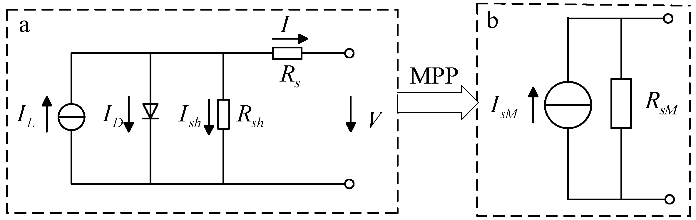
<p>Linear equivalent model of PV cell at the MPP.</p> "> Figure 3
<p>Equivalent model of PV system with battery.</p> "> Figure 4
<p>Equivalent model of PV system with supercapacitor.</p> "> Figure 5
<p>Structure of the whole system.</p> "> Figure 6
<p>Flow chart of the main control process.</p> "> Figure 7
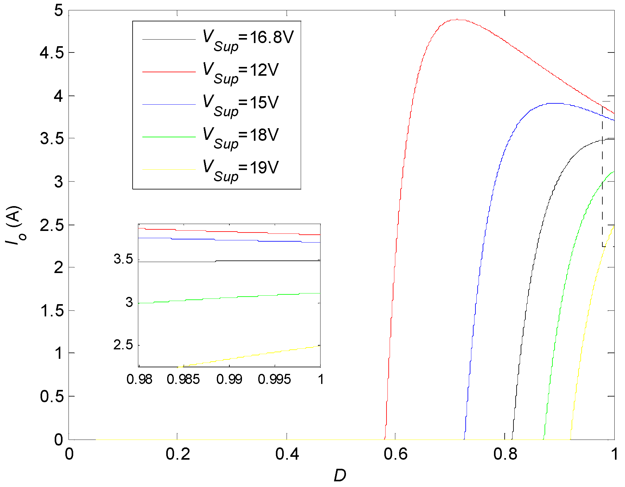
<p><math display="inline"><semantics> <mrow> <msub> <mi>I</mi> <mi>o</mi> </msub> <mo>−</mo> <mi>D</mi> </mrow> </semantics></math> curves with 400 W/m<sup>2</sup> and various <math display="inline"><semantics> <mrow> <msub> <mi>V</mi> <mrow> <mi>S</mi> <mi>u</mi> <mi>p</mi> </mrow> </msub> </mrow> </semantics></math> values.</p> "> Figure 8
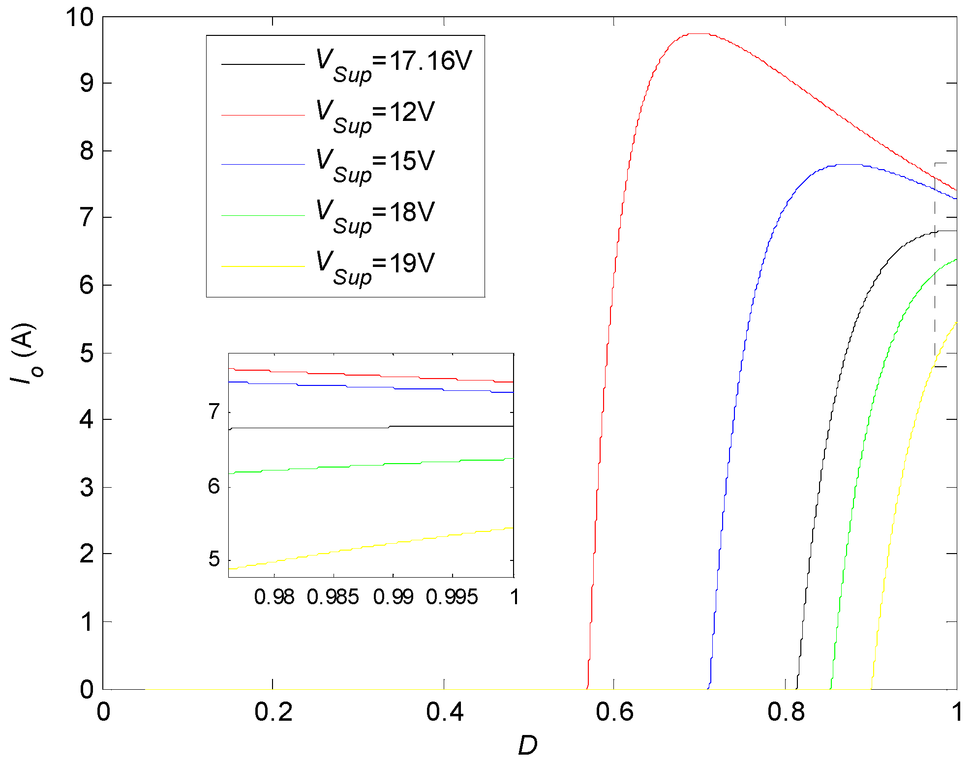
<p><math display="inline"><semantics> <mrow> <msub> <mi>I</mi> <mi>o</mi> </msub> <mo>−</mo> <mi>D</mi> </mrow> </semantics></math> curves with 600 W/m<sup>2</sup> and various <math display="inline"><semantics> <mrow> <msub> <mi>V</mi> <mrow> <mi>S</mi> <mi>u</mi> <mi>p</mi> </mrow> </msub> </mrow> </semantics></math> values.</p> "> Figure 9
<p><math display="inline"><semantics> <mrow> <msub> <mi>I</mi> <mi>o</mi> </msub> <mo>−</mo> <mi>D</mi> </mrow> </semantics></math> curves with 800 W/m<sup>2</sup> and various <math display="inline"><semantics> <mrow> <msub> <mi>V</mi> <mrow> <mi>S</mi> <mi>u</mi> <mi>p</mi> </mrow> </msub> </mrow> </semantics></math> values.</p> "> Figure 10
<p><math display="inline"><semantics> <mrow> <msub> <mi>I</mi> <mi>o</mi> </msub> <mo>−</mo> <mi>D</mi> </mrow> </semantics></math> curves with 1000 W/m<sup>2</sup> and various <math display="inline"><semantics> <mrow> <msub> <mi>V</mi> <mrow> <mi>S</mi> <mi>u</mi> <mi>p</mi> </mrow> </msub> </mrow> </semantics></math> values.</p> "> Figure 11
<p><math display="inline"><semantics> <mrow> <msub> <mi>I</mi> <mi>o</mi> </msub> <mo>−</mo> <mi>D</mi> </mrow> </semantics></math> curves under 0 °C and various <math display="inline"><semantics> <mrow> <msub> <mi>V</mi> <mrow> <mi>S</mi> <mi>u</mi> <mi>p</mi> </mrow> </msub> </mrow> </semantics></math> conditions.</p> "> Figure 12
<p><math display="inline"><semantics> <mrow> <msub> <mi>I</mi> <mi>o</mi> </msub> <mo>−</mo> <mi>D</mi> </mrow> </semantics></math> curves under 15 °C and various <math display="inline"><semantics> <mrow> <msub> <mi>V</mi> <mrow> <mi>S</mi> <mi>u</mi> <mi>p</mi> </mrow> </msub> </mrow> </semantics></math> conditions.</p> "> Figure 13
<p><math display="inline"><semantics> <mrow> <msub> <mi>I</mi> <mi>o</mi> </msub> <mo>−</mo> <mi>D</mi> </mrow> </semantics></math> curves under 30 °C and various <math display="inline"><semantics> <mrow> <msub> <mi>V</mi> <mrow> <mi>S</mi> <mi>u</mi> <mi>p</mi> </mrow> </msub> </mrow> </semantics></math> conditions.</p> "> Figure 14
<p><math display="inline"><semantics> <mrow> <msub> <mi>I</mi> <mi>o</mi> </msub> <mo>−</mo> <mi>D</mi> </mrow> </semantics></math> curves under 45 °C and various <math display="inline"><semantics> <mrow> <msub> <mi>V</mi> <mrow> <mi>S</mi> <mi>u</mi> <mi>p</mi> </mrow> </msub> </mrow> </semantics></math> conditions.</p> "> Figure 15
<p>Curve of <span class="html-italic">S</span> in first group.</p> "> Figure 16
<p>Compared curves of <math display="inline"><semantics> <mrow> <msub> <mi>P</mi> <mi>o</mi> </msub> </mrow> </semantics></math> in first group.</p> "> Figure 17
<p>Curve of <span class="html-italic">D</span> in first group.</p> "> Figure 18
<p>Curves of three currents in first group.</p> "> Figure 19
<p>Curve of <span class="html-italic">T</span> in second group.</p> "> Figure 20
<p>Curves of <math display="inline"><semantics> <mrow> <msub> <mi>P</mi> <mi>o</mi> </msub> </mrow> </semantics></math> in second group.</p> "> Figure 21
<p>Curve of <span class="html-italic">D</span> in second group.</p> "> Figure 22
<p>Curves of three currents in second group.</p> "> Figure 23
<p>Curve of <math display="inline"><semantics> <mrow> <msub> <mi>V</mi> <mrow> <mi>S</mi> <mi>u</mi> <mi>p</mi> </mrow> </msub> </mrow> </semantics></math> in third group.</p> "> Figure 24
<p>Curves of <math display="inline"><semantics> <mrow> <msub> <mi>P</mi> <mi>o</mi> </msub> </mrow> </semantics></math> in third group.</p> "> Figure 25
<p>Curve of <span class="html-italic">D</span> in third group.</p> "> Figure 26
<p>Curves of three currents in third group.</p> "> Figure 27
<p>Curve of the varying irradiance.</p> "> Figure 28
<p>Curve of the varying temperature.</p> "> Figure 29
<p>Compared duty cycle curves of three MPPT methods.</p> "> Figure 30
<p>Compared power curves of three MPPT methods.</p> "> Figure 31
<p>Compared output current curves of three MPPT methods.</p> "> Figure 32
<p>Compared curves of <math display="inline"><semantics> <mrow> <msub> <mi>I</mi> <mrow> <mi>s</mi> <mi>M</mi> </mrow> </msub> </mrow> </semantics></math> and <math display="inline"><semantics> <mrow> <mn>2</mn> <msub> <mi>I</mi> <mrow> <mi>o</mi> <mi>M</mi> </mrow> </msub> </mrow> </semantics></math>.</p> ">
Abstract
:1. Introduction
- (1)
- The MPPT constraint conditions of a PV system with a battery or supercapacitor are successfully found. This work is the first attempt to study this issue on the basis of the current relationships.
- (2)
- An MPPT control strategy is proposed. This work is the first attempt to design the MPPT strategy by using both proposed MPPT constraint conditions and an output current limitation.
- (3)
- The thought on three operating modes is proposed to design the control process. It is the key to implementing this proposed MPPT strategy without sampling any current data. Meanwhile, it is also the key to simplifying the whole control process, reducing the microprocessor cost, and shortening the whole design period.
- (4)
- Some equations corresponding to every mode are built to directly calculate the real-time control signal. They are the key to ensuring the good MPPT speed of this proposed MPPT strategy.
- (5)
- By this work, the MPPT constraint conditions based on current relationships are first found and the calculated control signal can be directly obtained in real time, which establishes a strong foundation for the later designing and application of a PV system with a battery or supercapacitor.
2. Materials and Methods
2.1. Principle
2.1.1. Mathematical Relationships between Currents and Control Signal
2.1.2. Mathematical Relationships around the MPP
2.1.3. Constraint Conditions Based on Currents
2.2. Proposition
2.3. Implementation
2.3.1. System Structure and Control Process
2.3.2. Acquisition of the Main Parameters
3. Results
3.1. Analysis for the MPPT Constraint Conditions
3.1.1. Results under Different Irradiance Conditions
3.1.2. Results under Different Temperature Conditions
3.2. Verification of the Whole Control Process
3.2.1. Results under Different Irradiance Conditions
3.2.2. Results under Different Temperature Conditions
3.2.3. Results under Different Supercapacitor Voltage Conditions
3.3. Comparison
4. Discussions
5. Conclusions
Author Contributions
Funding
Data Availability Statement
Acknowledgments
Conflicts of Interest
Abbreviations and Nomenclature
| MPPT | maximum power point tracking | MPP voltage of PV cell at STC (V) | |
| PV | photovoltaic | output voltage of the DC/DC converter (V) | |
| MPP | maximum power point | output current of the DC/DC converter (A) | |
| VWP | variable weather parameter | output voltage of PV cell (V) | |
| P&O | perturbation and observation | output current of PV cell (A) | |
| SMC | sliding mode control | voltage of battery (V) | |
| ANN | artificial neural network | voltage of supercapacitor (V) | |
| INC | incremental conductance | output power corresponding to the MPP (W) | |
| PSO | particle swarm optimization | upper value of the charging power (W) | |
| ANFIS | adaptive neuro-fuzzy inference system | upper value of the charging current (A) | |
| SOC | state of charge | corresponding to the MPP (A) | |
| THD | total harmonic distortion | corresponding to the MPP (V) | |
| PWM | pulse–width modulation | corresponding to the MPP (V) | |
| DC | direct current | corresponding to the MPP (A) | |
| STC | standard test conditions | internal resistance of linear cell model (Ω) | |
| PI | proportional integral | short-circuit current of linear cell model (A) | |
| PID | proportional integral derivative | D | duty cycle of the PWM signal of the converter |
| short-circuit current of PV cell at STC (A) | D corresponding to the MPP | ||
| open-circuit voltage of PV cell at STC (V) | S | solar irradiance (W/m2) | |
| MPP current of PV cell at STC (A) | T | cell temperature (°C) |
References
- Du, Y.; Lu, D.D.C. Battery-integrated boost converter utilizing distributed MPPT configuration for photovoltaic systems. Sol. Energy 2011, 85, 1992–2002. [Google Scholar] [CrossRef]
- Alahmadi, A.N.M.; Rezk, H. A robust single-sensor MPPT strategy for shaded photovoltaic-battery system. Comput. Syst. Sci. Eng. 2021, 37, 63–71. [Google Scholar] [CrossRef]
- Ali, S.U.; Waqar, A.; Aamir, M.; Qaisar, S.M.; Iqbal, J. Model predictive control of consensus-based energy management system for DC microgrid. PLoS ONE 2023, 20, 0278110. [Google Scholar] [CrossRef] [PubMed]
- Şahin, M.E.; Blaabjerg, F. PV powered hybrid energy storage system control using bidirectional and boost converters. Electr. Power Compon. Syst. 2022, 49, 1260–1277. [Google Scholar] [CrossRef]
- Abousserhane, Z.; Abbou, A.; Bouzakri, H. Developed power flow control of PV/battery/SC hybrid storage system featuring two grid modes. Int. J. Renew. Energy Res. 2022, 12, 190–199. [Google Scholar]
- Kord, H.; Zamani, A.A.; Barakati, S.M. Active hybrid energy storage management in a wind-dominated standalone system with robust fractional-order controller optimized by gases brownian motion optimization algorithm. J. Energy Storage 2023, 66, 107492. [Google Scholar] [CrossRef]
- Chellakhi, A.; El Beid, S.; Abouelmahjoub, Y. An improved adaptable step-size P&O MPPT approach for standalone photovoltaic systems with battery station. Simul. Model. Pract. Theory 2022, 121, 102655. [Google Scholar]
- Chtita, S.; Motahhir, S.; El Ghzizal, A. A new design and embedded implementation of a low-cost maximum power point tracking charge controller for stand-alone photovoltaic systems. Energy Technol. 2024, 12, 202301324. [Google Scholar] [CrossRef]
- Chahar, S.; Razzaq, A. P&O and incremental conductance MPP tracking for solar PV array: A comparative ideal data and real-time study. J. Act. Passiv. Electron. Devices 2023, 17, 269–286. [Google Scholar]
- El Mezdi, K.; El Magri, A.; Watil, A.; El Myasse, I.; Bahatti, L.; Lajouad, R.; Ouabi, H. Nonlinear control design and stability analysis of hybrid grid-connected photovoltaic-battery energy storage system with ANN-MPPT method. J. Energy Storage 2023, 72, 108747. [Google Scholar] [CrossRef]
- Siddaraj, S.; Yaragatti, U.R.; Harischandrappa, N. Coordinated PSO-ANFIS-Based 2 MPPT control of microgrid with solar photovoltaic and battery energy storage system. J. Sens. Actuator Netw. 2023, 12, 45. [Google Scholar] [CrossRef]
- Fekik, A.; Hamida, M.L.; Azar, A.T.; Ghanes, M.; Hakim, A.; Denoun, H.; Hameed, I.A. Robust power control for photovoltaic and battery systems: Integrating sliding mode MPPT with dual buck converters. Front. Energy Res. 2024, 12, 1380387. [Google Scholar] [CrossRef]
- Zehra, S.S.; Rahman, A.U.; Armghan, H.; Ahmad, I.; Ammara, U. Artificial intelligence-based nonlinear control of renewable energies and storage system in a DC microgrid. ISA Trans. 2022, 121, 217–231. [Google Scholar] [CrossRef] [PubMed]
- Haroon, F.; Aamir, M.; Waqar, A.; Qaisar, S.M.; Ali, S.U.; Almaktoom, A.T. A composite exponential reaching law based SMC with rotating sliding surface selection mechanism for two level three phase VSI in vehicle to load applications. Energies 2023, 16, 346. [Google Scholar] [CrossRef]
- Pan, Z.; Quynh, N.V.; Ali, Z.M.; Dadfar, S.; Kashiwagi, T. Enhancement of maximum power point tracking technique based on PV-battery system using hybrid BAT algorithm and fuzzy controller. J. Clean. Prod. 2020, 274, 123719. [Google Scholar] [CrossRef]
- Sandeep, S.D.; Mohanty, S. Artificial rabbits optimized neural network-based energy management system for PV, battery, and supercapacitor based isolated DC microgrid system. IEEE Access 2023, 11, 142411–142432. [Google Scholar]
- Li, S.; Ping, A.; Liu, Y.; Ma, X.; Li, C. A variable-weather-parameter MPPT method based on a defined characteristic resistance of photovoltaic cell. Sol. Energy 2020, 199, 673–684. [Google Scholar] [CrossRef]
- Li, S. A variable-weather-parameter MPPT control strategy based on MPPT constraint conditions of PV system with inverter. Energy Convers. Manag. 2019, 197, 111873. [Google Scholar] [CrossRef]
- Goud, J.S.; Kalpana, R.; Singh, B.; Kumar, S. A global maximum power point tracking technique of partially shaded photovoltaic systems for constant voltage applications. IEEE Trans. Sustain. Energy 2019, 10, 1950–1959. [Google Scholar] [CrossRef]
- Roy, T.K.; Oo, A.M.T.; Ghosh, S.K. Designing a high-order sliding mode controller for photovoltaic and battery energy storage system-based DC microgrids with ANN-MPPT. Energies 2024, 17, 17020532. [Google Scholar] [CrossRef]
- Agoub, R.A.A.; Hançerlioğullari, A.; Rahebi, J.; Lopez-Guede, J.M. Battery charge control in solar photovoltaic systems based on fuzzy logic and jellyfish optimization algorithm. Appl. Sci. 2023, 13, 11409. [Google Scholar] [CrossRef]
- Fu, Z.; Fan, Y.; Cai, X.; Zheng, Z.; Xue, J.; Zhang, K. Lithium titanate battery management system based on MPPT and four-stage charging control for photovoltaic energy storage. Appl. Sci. 2019, 8, 2520. [Google Scholar] [CrossRef]
- Li, S. MPPT constraint conditions based on four-parameter cell model for some usual photovoltaic systems. Sustain. Energy Technol. Assess. 2024, 68, 103874. [Google Scholar] [CrossRef]
- Jordehi, A.R. Parameter estimation of solar photovoltaic (PV) cells: A review. Renew. Sustain. Energy Rev. 2016, 61, 354–371. [Google Scholar] [CrossRef]
- Mutoh, N.; Ohno, M.; Inoue, T. A method for MPPT control while searching for parameters corresponding to weather conditions for PV generation systems. IEEE Trans. Ind. Electron. 2006, 53, 1055–1065. [Google Scholar] [CrossRef]
- Li, Q.; Zhao, S.; Wang, M.; Zou, Z.; Wang, B.; Chen, Q. An improved perturbation and observation maximum power point tracking algorithm based on a PV module four-parameter model for higher efficiency. Appl. Energy 2017, 195, 523–537. [Google Scholar] [CrossRef]
- Gopi, R.R.; Sreejith, S. Converter topologies in photovoltaic applications—A review. Renew. Sustain. Energy Rev. 2018, 94, 1–14. [Google Scholar] [CrossRef]
- Li, S. Linear equivalent models at the maximum power point based on variable weather parameters for photovoltaic cell. Appl. Energy 2016, 182, 94–104. [Google Scholar] [CrossRef]


(V) | (A) | (A) | (A) | (A) | (A) | (A) | (A) | (A) | (A) | (A) |
|---|---|---|---|---|---|---|---|---|---|---|
| 5 | 6.9809 | 23.4548 | 10.4713 | 34.6537 | 13.9617 | 46.5220 | 17.4522 | 59.8011 | 20.9426 | 75.1229 |
| 6 | 6.9809 | 15.5457 | 10.4713 | 28.8781 | 13.9617 | 38.7683 | 17.4522 | 49.8343 | 20.9426 | 62.6024 |
| 7 | 6.9809 | 16.7534 | 10.4713 | 24.7526 | 13.9617 | 33.2300 | 17.4522 | 42.7151 | 20.9426 | 53.6592 |
| 8 | 6.9809 | 14.6592 | 10.4713 | 21.6585 | 13.9617 | 29.0762 | 17.4522 | 37.3757 | 20.9426 | 46.9518 |
| 9 | 6.9809 | 13.0304 | 10.4713 | 19.2520 | 13.9617 | 25.8455 | 17.4522 | 33.2228 | 20.9426 | 41.7349 |
| 10 | 6.9809 | 11.7274 | 10.4713 | 17.3268 | 13.9617 | 23.2610 | 17.4522 | 29.9006 | 20.9426 | 37.5615 |
| 11 | 6.9809 | 10.6613 | 10.4713 | 15.7517 | 13.9617 | 21.1464 | 17.4522 | 27.1823 | 20.9426 | 34.1468 |
| 12 | 6.9809 | 9.7728 | 10.4713 | 14.4390 | 13.9617 | 19.3842 | 17.4522 | 24.9171 | 20.9426 | 31.3012 |
| 13 | 6.9809 | 9.0211 | 10.4713 | 13.3283 | 13.9617 | 17.8931 | 17.4522 | 23.0004 | 20.9426 | 28.8934 |
| 14 | 6.9809 | 8.3767 | 10.4713 | 12.3763 | 13.9617 | 16.6150 | 17.4522 | 21.3575 | 20.9426 | 26.8296 |
| 15 | 6.9809 | 7.8183 | 10.4713 | 11.5512 | 13.9617 | 15.5073 | 17.4522 | 19.9337 | 20.9426 | 25.0410 |
| 16 | 6.9809 | 7.3296 | 10.4713 | 10.8293 | 13.9617 | 14.5381 | 17.4522 | 18.6878 | 20.9426 | 23.4759 |
| 17 | 6.9809 | 6.8919 | 10.4713 | 10.1377 | 13.9617 | 13.6435 | 17.4522 | 17.5886 | 20.9426 | 22.0950 |
| 18 | 6.9809 | 6.2287 | 10.4713 | 8.9383 | 13.9617 | 12.1744 | 17.4522 | 16.2768 | 20.9426 | 20.8657 |
| 19 | 6.9809 | 4.9680 | 10.4713 | 6.6355 | 13.9617 | 9.3664 | 17.4522 | 13.8263 | 20.9426 | 19.2006 |
| 20 | 6.9809 | 2.5710 | 10.4713 | 2.2144 | 13.9617 | 3.9992 | 17.4522 | 9.2252 | 20.9426 | 16.1611 |
(V) | (A) | (A) | (A) | (A) | (A) | (A) | (A) | (A) | (A) | (A) |
|---|---|---|---|---|---|---|---|---|---|---|
| 5 | 12.6160 | 47.0993 | 13.1207 | 47.0094 | 13.6253 | 46.7675 | 14.1300 | 46.3739 | 14.6346 | 45.8284 |
| 6 | 12.6160 | 39.2495 | 13.1207 | 39.1745 | 13.6253 | 38.9730 | 14.1300 | 38.6449 | 14.6346 | 38.1903 |
| 7 | 12.6160 | 33.6424 | 13.1207 | 33.5781 | 13.6253 | 33.4054 | 14.1300 | 33.1242 | 14.6346 | 32.7346 |
| 8 | 12.6160 | 29.4371 | 13.1207 | 29.3809 | 13.6253 | 29.2297 | 14.1300 | 28.9837 | 14.6346 | 28.6427 |
| 9 | 12.6160 | 26.1663 | 13.1207 | 26.1163 | 13.6253 | 25.9820 | 14.1300 | 25.7633 | 14.6346 | 25.4602 |
| 10 | 12.6160 | 23.5497 | 13.1207 | 23.5047 | 13.6253 | 23.3838 | 14.1300 | 23.1869 | 14.6346 | 22.9142 |
| 11 | 12.6160 | 21.4088 | 13.1207 | 21.3679 | 13.6253 | 21.2580 | 14.1300 | 21.0790 | 14.6346 | 20.8311 |
| 12 | 12.6160 | 19.6247 | 13.1207 | 19.5872 | 13.6253 | 19.4865 | 14.1300 | 19.3224 | 14.6346 | 19.0952 |
| 13 | 12.6160 | 18.1151 | 13.1207 | 18.0805 | 13.6253 | 17.9875 | 14.1300 | 17.8361 | 14.6346 | 17.6263 |
| 14 | 12.6160 | 16.8212 | 13.1207 | 16.7891 | 13.6253 | 16.7027 | 14.1300 | 16.5621 | 14.6346 | 16.3673 |
| 15 | 12.6160 | 15.6998 | 13.1207 | 15.6698 | 13.6253 | 15.5892 | 14.1300 | 15.4580 | 14.6346 | 15.2761 |
| 16 | 12.6160 | 14.7185 | 13.1207 | 14.6904 | 13.6253 | 14.6149 | 14.1300 | 14.4918 | 14.6346 | 14.2735 |
| 17 | 12.6160 | 13.8528 | 13.1207 | 13.8263 | 13.6253 | 13.7552 | 14.1300 | 13.5089 | 14.6346 | 12.5695 |
| 18 | 12.6160 | 13.0832 | 13.1207 | 13.0562 | 13.6253 | 12.7493 | 14.1300 | 11.7129 | 14.6346 | 9.1745 |
| 19 | 12.6160 | 12.3674 | 13.1207 | 11.9979 | 13.6253 | 10.8769 | 14.1300 | 8.2460 | 14.6346 | 2.4103 |
| 20 | 12.6160 | 11.2576 | 13.1207 | 10.0647 | 13.6253 | 7.3651 | 14.1300 | 1.5533 | 14.6346 | 0 |
) | (A) | (A) | (W) | (W) | ) | (A) | ||
|---|---|---|---|---|---|---|---|---|
| 400 | 6.7287 | 6.7648 | 58.52 | 138.40 | 0.9947 | / | / | 3.4126 |
| 450 | 7.5697 | 7.5754 | 65.53 | 138.40 | 0.9993 | / | / | 3.8175 |
| 500 | 8.4108 | 8.3916 | 72.59 | 138.40 | / | 1 | / | 4.2239 |
| 550 | 9.2519 | 9.2161 | 79.72 | 138.40 | / | 1 | / | 4.6323 |
| 600 | 10.0930 | 10.0514 | 86.94 | 138.40 | / | 1 | / | 5.0447 |
| 650 | 10.9341 | 10.9000 | 94.29 | 138.40 | / | 1 | / | 5.4631 |
| 700 | 11.7751 | 11.7645 | 101.76 | 138.40 | / | 1 | / | 5.8894 |
| 750 | 12.6162 | 12.6474 | 109.40 | 138.40 | 0.9975 | / | / | 6.3252 |
| 800 | 13.4573 | 13.5513 | 117.22 | 138.40 | 0.9931 | / | / | 6.7724 |
| 850 | 14.2984 | 14.4787 | 125.24 | 138.40 | 0.9875 | / | / | 7.2324 |
| 900 | 15.1395 | 15.4322 | 133.49 | 138.40 | 0.9810 | / | / | 7.7070 |
| 950 | 15.9806 | 16.4143 | 141.98 | 138.40 | / | / | 0.9240 | 8.0000 |
| 1000 | 16.8216 | 17.4276 | 150.75 | 138.40 | / | / | 0.8843 | 8.0000 |
| 1050 | 17.6627 | 18.4747 | 159.81 | 138.40 | / | / | 0.8594 | 8.0000 |
| 1100 | 18.5038 | 19.5580 | 169.18 | 138.40 | / | / | 0.8391 | 8.0000 |
| 1150 | 19.3449 | 20.6802 | 178.88 | 138.40 | / | / | 0.8211 | 8.0000 |
| 1200 | 20.1859 | 21.8438 | 188.95 | 138.40 | / | / | 0.8043 | 8.0000 |
| T (°C) | (A) | (A) | (W) | (W) | ) | (A) | ||
|---|---|---|---|---|---|---|---|---|
| 0 | 14.6664 | 16.1479 | 139.68 | 138.40 | / | / | 0.8888 | 8.0000 |
| 5 | 14.8619 | 16.1219 | 139.45 | 138.40 | / | / | 0.9015 | 8.0000 |
| 10 | 15.0575 | 16.0959 | 139.23 | 138.40 | / | / | 0.9155 | 8.0000 |
| 15 | 15.2530 | 16.0699 | 139.00 | 138.40 | / | / | 0.9311 | 8.0000 |
| 20 | 15.4486 | 16.0439 | 138.78 | 138.40 | / | / | 0.9492 | 8.0000 |
| 25 | 15.6441 | 16.0179 | 138.55 | 138.40 | / | / | 0.9761 | 8.0000 |
| 30 | 15.8397 | 15.9918 | 138.33 | 138.40 | 0.9905 | / | / | 7.9826 |
| 35 | 16.0352 | 15.9658 | 138.10 | 138.40 | / | 1 | / | 7.9608 |
| 40 | 16.2308 | 15.9398 | 137.88 | 138.40 | / | 1 | / | 7.9140 |
| 45 | 16.4263 | 15.9138 | 137.65 | 138.40 | / | 1 | / | 7.8323 |
| 50 | 16.6219 | 15.8878 | 137.43 | 138.40 | / | 1 | / | 7.7063 |
() | (A) | (A) | (W) | (W) | ) | (A) | ||
|---|---|---|---|---|---|---|---|---|
| 8 | 10.0930 | 21.7362 | 86.94 | 64.00 | / | / | 0.4033 | 8.0000 |
| 9 | 10.0930 | 19.3210 | 86.94 | 72.00 | / | / | 0.4623 | 8.0000 |
| 10 | 10.0930 | 17.3889 | 86.94 | 80.00 | / | / | 0.5287 | 8.0000 |
| 11 | 10.0930 | 15.8081 | 86.94 | 88.00 | 0.6385 | / | / | 7.9332 |
| 12 | 10.0930 | 14.4908 | 86.94 | 96.00 | 0.6965 | / | / | 7.2721 |
| 13 | 10.0930 | 13.3761 | 86.94 | 104.00 | 0.7546 | / | / | 6.7127 |
| 14 | 10.0930 | 12.4207 | 86.94 | 112.00 | 0.8126 | / | / | 6.2332 |
| 15 | 10.0930 | 11.5926 | 86.94 | 120.00 | 0.8706 | / | / | 5.8177 |
| 16 | 10.0930 | 10.8681 | 86.94 | 128.00 | 0.9287 | / | / | 5.4541 |
| 17 | 10.0930 | 10.2288 | 86.94 | 136.00 | 0.9867 | / | / | 5.1332 |
| 18 | 10.0930 | 9.6605 | 86.94 | 144.00 | / | 1 | / | 4.7876 |
| 19 | 10.0930 | 9.1521 | 86.94 | 152.00 | / | 1 | / | 4.1580 |
| 20 | 10.0930 | 8.6945 | 86.94 | 160.00 | / | 1 | / | 2.9830 |
| Time Intervals (s) | [0.0, 0.1] | [0.1, 0.2] | [0.2, 0.3] | [0.3, 0.4] | [0.4, 0.5] | [0.5, 0.6] | [0.6, 0.7] | [0.7, 0.8] | [0.8, 0.9] | [0.9, 1.0] |
|---|---|---|---|---|---|---|---|---|---|---|
| S (W/m2) | 400 | 1195 | 470 | 1000 | 525 | 925 | 690 | 400 | 799 | 1195 |
| T (°C) | 4.4 | 40.2 | 0.8 | 19.8 | 43.2 | 30.0 | 14.4 | 5.6 | 26.6 | 49.8 |
| (A) | 6.3821 | 20.8657 | 7.4278 | 16.6030 | 9.2331 | 15.7545 | 11.2993 | 6.4023 | 13.4943 | 21.3482 |
| (A) | 7.9256 | 24.9656 | 9.2578 | 20.1311 | 10.0433 | 18.3305 | 13.4309 | 7.9184 | 15.5984 | 24.9080 |
| (A) | 3.9567 | 12.4498 | 4.6140 | 10.0582 | 5.0577 | 9.1500 | 6.7148 | 3.9563 | 7.7972 | 12.3661 |
| (A) | / | / | / | / | / | 9.1501 | 6.7147 | 3.9562 | 7.7888 | 12.3697 |
| (A) | 3.9567 | 12.4503 | 4.6143 | 10.0582 | 5.0594 | 9.1507 | 6.7147 | 3.9563 | 7.7873 | 12.3698 |
| (W) | 59.3513 | 186.7545 | 69.2147 | 150.8735 | 75.8919 | 137.2530 | 100.7248 | 59.3448 | 116.9325 | 185.5479 |
| (W) | 59.3504 | 186.7469 | 69.2107 | 150.8726 | 75.8671 | 137.2460 | 100.7247 | 59.3438 | 116.9110 | 185.4907 |
| (W) | / | / | / | / | / | 137.2507 | 100.7131 | 59.3415 | 116.7987 | 185.5477 |
| (W) | 59.3497 | 186.7534 | 69.2147 | 150.8726 | 75.8905 | 137.2504 | 100.7216 | 59.3437 | 116.8060 | 185.5478 |
| 0.8053 | 0.8358 | 0.8023 | 0.8247 | 0.9193 | 0.8595 | 0.8413 | 0.8085 | 0.8651 | 0.8571 | |
| / | / | / | / | / | 0.8610 | 0.8415 | 0.8100 | 0.8655 | 0.8625 | |
| 0.8060 | 0.8361 | 0.8040 | 0.8244 | 0.9120 | 0.8605 | 0.8412 | 0.8085 | 0.8655 | 0.8622 | |
| (ms) | 6 | 3 | 3.5 | 3.5 | 3.8 | 3.8 | 4 | 3.5 | 3.8 | 4.5 |
| (ms) | / | / | / | / | / | 75 | 12 | 18 | 33 | 11 |
| (ms) | 68 | 7 | 7 | 6.5 | 20 | 27 | 6 | 5.5 | 8 | 10 |
| Methods or Works | Main Advantages | Main Shortcomings | Key Findings or Thoughts |
|---|---|---|---|
| Proposed method | (1) fastest MPPT speed; (2) simple control process; (3) low hardware cost and short design period. | use of irradiance and temperature sensors | (1) MPPT constraint conditions based on currents; (2) thoughts of three operating modes and switching among them; (3) techniques of directly calculating the control signal to match three operating modes. |
| work in Ref. [8] | (1) low cost; (2) strong robustness. | relatively complex control process | (1) avoiding all mathematical division in conventional INC algorithm; (2) a designed feedback control based on two PI compensators. |
| work in Ref. [16] | (1) good voltage steadiness of DC bus; (2) minimized battery stress. | complex algorithm involving in high-cost microprocessor and slower MPPT speed | (1) power losses considered during design; (2) artificial rabbit-optimized neural network combined with INC algorithm. |
| work in Ref. [20] | (1) strong robustness; (2) good performance. | high-cost microprocessor arising from complex algorithm and slower MPPT speed | (1) a combination of PID, SMC, and ANN algorithms; (2) use of Lyapunov stability theory. |
| work in Ref. [23] | (1) relatively complete findings for MPPT constraint conditions; (2) an involvement with four parameter cell model. | No consideration for relationships between currents | (1) MPPT constraint conditions based on voltages; (2) MPPT constraint relationships among circuit parameters, cell parameters, and load. |
Disclaimer/Publisher’s Note: The statements, opinions and data contained in all publications are solely those of the individual author(s) and contributor(s) and not of MDPI and/or the editor(s). MDPI and/or the editor(s) disclaim responsibility for any injury to people or property resulting from any ideas, methods, instructions or products referred to in the content. |
© 2024 by the authors. Licensee MDPI, Basel, Switzerland. This article is an open access article distributed under the terms and conditions of the Creative Commons Attribution (CC BY) license (https://creativecommons.org/licenses/by/4.0/).
Share and Cite
Lai, G.; Zhang, G.; Li, S. An MPPT Control Strategy Based on Current Constraint Relationships for a Photovoltaic System with a Battery or Supercapacitor. Energies 2024, 17, 3982. https://doi.org/10.3390/en17163982
Lai G, Zhang G, Li S. An MPPT Control Strategy Based on Current Constraint Relationships for a Photovoltaic System with a Battery or Supercapacitor. Energies. 2024; 17(16):3982. https://doi.org/10.3390/en17163982
Chicago/Turabian StyleLai, Guohong, Guoping Zhang, and Shaowu Li. 2024. "An MPPT Control Strategy Based on Current Constraint Relationships for a Photovoltaic System with a Battery or Supercapacitor" Energies 17, no. 16: 3982. https://doi.org/10.3390/en17163982