|
We propose a pipeline to acquire a scalar tapering measurement from the carina to the most distal point of an individual airway visible on computed tomography (CT). We show the applicability of using tapering measurements on clinically acquired data by quantifying the reproducibility of the tapering measure. We generate a spline from the centerline of an airway to measure the area and arclength at contiguous intervals. The tapering measurement is the gradient of the linear regression between area in log space and arclength. The reproducibility of the measure was assessed by analyzing different radiation doses, voxel sizes, and reconstruction kernel on single timepoint and longitudinal CT scans and by evaluating the effect of airway bifurcations. Using 74 airways from 10 CT scans, we show a statistical difference, p = 3.4 × 10 − 4, in tapering between healthy airways (n = 35) and those affected by bronchiectasis (n = 39). The difference between the mean of the two populations is 0.011 mm − 1, and the difference between the medians of the two populations was 0.006 mm − 1. The tapering measurement retained a 95% confidence interval of ±0.005 mm − 1 in a simulated 25 mAs scan and retained a 95% confidence of ±0.005 mm − 1 on simulated CTs up to 1.5 times the original voxel size. We have established an estimate of the precision of the tapering measurement and estimated the effect on precision of the simulated voxel size and CT scan dose. We recommend that the scanner calibration be undertaken with the phantoms as described, on the specific CT scanner, radiation dose, and reconstruction algorithm that are to be used in any quantitative studies. |
1.Introduction and PurposeBronchiectasis is defined as the permanent dilatation of the airways. Patients with bronchiectasis can suffer severe exacerbations requiring hospital admission and have a poorer quality of life.1 Clinicians diagnose bronchiectasis on computed tomography (CT) imaging by visually estimating the diameter of the airway/bronchus and its adjacent pulmonary artery and calculating the broncho-arterial (BA) ratio. A BA ratio indicates the presence of bronchiectasis.2 Various groups have proposed methods to automatically and semiautomatically compute the BA ratio for bronchiectatic airways.3–5 However, use of the BA ratio to diagnose bronchiectasis has two major flaws. First of all, the maximum healthy range of the BA ratio can be 1.5 times size of the artery.6 Second, blood vessels can change size as a result of factors including altitude,7 patient age,8 and smoking status.9 This conflicts with the assumption that the pulmonary artery is always at a constant size. An alternative approach to diagnose and monitor bronchiectatic airways is to analyze the taper of the airways, i.e., the rate of change in the cross-sectional area along the airway.2 In patients with bronchiectasis, the airway is dilated and so the tapering rate must be reduced. Airway tapering is difficult to assess visually and to measure manually. As described by Hansell,6 the observer would have to make multiple cross-sectional area measurements along the airway. As mentioned by Cheplygina et al,10 measuring multiple lumen is a manually exhaustive task and prone to mistakes. 1.1.Related WorkThere have been various strategies to quantify tapering in the airways. The initial proposed tapering measurements by Odry et al.11 were restricted to short lengths of the airways. A segmented airway would be split into four equal parts. Each segment had an array of computed lumen diameters. The tapering was measured as the linear regression of the lumen diameters along the branch. The method shared similarity to Venkatraman et al.,12 but the diameter measurements were taken across the central half of each branch. Various analyses attempted to measure the taper of airways containing multiple branches. In the work of Oguma et al.,13 the region of interest from the carina to the fifth generation airway was measured; however, this was only performed in patients with COPD. Finally, Weinheimer et al.14 used a graphical model of the airways for their proposed tapering measurement. The graphical model was based on a graphical tree originating at the trachea and extending into distal branches, depending on airway bifurcations. A tapering measure was assigned to the edge of the graph depending on the lumen area and generation. They also proposed a regional tapering measurement based on the segments of the lobes of the lungs. The described tapering measurements have two key limitations. First of all, there is no detailed quantification of reproducibility when considering differences in specifications of the CT scanner, or reconstruction kernel, making it difficult to compare tapering statistics from different machines or from the same CT scanner employing different scanning parameters. Second, the region of interest for the tapering measurement was restricted to airways that were segmented using the respective airway segmentation software. Bronchiectasis is a heterogeneous disease—it can affect any area in the lung including the peripheral regions.15 Thus to encapsulate the disease in the tapering measurement, one would need to consider the region of interest as the entire airway, from the trachea to the most distal point. In all the proposed tapering measurements, obtaining the cross-sectional area is a necessary input for the algorithms. There have been various analyses attempting to validate the reproducibility and precision of measurements against dose,16–18 voxel size,19 reconstruction kernel,20–22 and normal biological variation.23 In most of the validation experiments, area measurements were taken from phantom,20,21 porcine,16,18 or cadaver24 models. Fetita et al.25 used synthetic models of the lung. None of these experiments were explicitly performed on scans with bronchiectasis. Furthermore, the area measurements were not taken at contiguous intervals along the lumen thus missing possible dilatations from a bronchiectatic airway. For our work and the method from Oguma et al.,13 the tapering measurement involves the computation of the arc length of the airway at contiguous intervals. In the literature, investigations of the reproducibility of arc length computation in airways are limited. The work of Palágyi et al.26 used simulated rotation of in vivo scans. The assessment of the reproducibility was based on the lengths of a single branch rather than multiple generations of branches, thereby precluding estimations of reproducibility of airway quantitation from the carina to an airway’s most distal point. 1.2.Contributions of the PaperTo our knowledge, there is no detailed analysis on the reproducibility of a global tapering measurement of airways using CT. Thus the purpose of this paper is as follows. First of all, we will discuss in detail a tapering measurement of the airways on CT imaging. Second, we quantify the reproducibility of the measurement against variations in simulated dose and voxel sizes. In addition, we compare the variability of the tapering measurements across different CT reconstructions kernel. Finally, we analyze the effect of bifurcations on tapering measurements and consider measurement repeatability using longitudinal scans. 2.MethodWe first describe in detail the steps to acquire the airway tapering measurement. The method was initially proposed by Quan et al.27; it is summarized in Fig. 1. The pipeline required two inputs. First, the most distal point of each airway of interest was manually identified by an experienced radiologist (J. J.). A single voxel was marked at the end of the airway centerline. The entire analysis was completed using ITK-SNAP.28 Fig. 1Summary of steps in our pipeline: (a) airway segmentation, (b) centerline computation, (c) reconstruct planes on the centerline spline, (d) lumen identification via ray casting, (e) lumen area along the airway, and (f) area profile in log space with line of best fit. 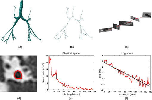 Second, a complete segmentation of the airway was produced. We obtained an airway segmentation by implementing a method developed by van Rikxoort et al.29 The algorithm was based on a region growing paradigm. In summary, a wave front was initialized from the trachea. Voxels on each new iteration were classed as airways based on a voxel criterion. The wave front continued until a wave front criteria was met. In certain cases, the airway segmentation was unable to reach the distal points, and, in these cases, we extended the airway segmentation manually to the distal points. Our method is designed so that it can be incorporated to any system that provides both the segmentation and distal point to the airway of interest. Once the inputs were available, we acquired the measurement using an automatic process. 2.1.CenterlineThe centerline was used to identify and order the airway segments for the tapering measurement. We implemented a curve thinning algorithm developed by Palágyi et al.26 At initialization, the algorithm used the airway segmentation and distal points acquired in Sec. 2. The final input was the start of the centerline at the trachea. The shape of the trachea was assumed to be tubular, with an approximate constant diameter and orientated near perpendicular to the axial slice. Thus the centerline of the trachea lay on the local maximum value of the distance transform of the segmented trachea.30 Algorithm 1 was used to find the centerline start point. Algorithm 1Locating the start of centerline on the trachea.
2.2.Recentering and Spline FittingThe next task was to separate the centerline of each individual airway from the centerline tree. To this end, we modeled the centerline tree as a graphical model similar to Mori et al.31 The nodes corresponded to the centerline voxels and the edges linked neighboring voxels. We performed a breadth first search algorithm32 on the centerline image. Starting from the carina, we iteratively found the next set of sibling branches. When a distal point was found at the end of a parent branch, the path leading to the distal point was saved. The output was an array of ordered paths describing the unique route from the trachea to the distal point. The proposed tapering measurement started at the carina. Thus centerline points corresponding to the trachea were removed from further analysis. For each path, we corrected for the discretization error—a process known as recentering.33 We implemented a similar method to that described by Irving et al.34 A five point smoothing was performed along each path. We modeled the centerline as a continuous model by fitting a cubic spline denoted as where and . The knots where taken on every smoothed point on the centerline. The spline fitting was performed using the cscvn35 function in MATLAB. The continuous model should enable computations of the arc length and tangent at subvoxel intervals along the airway.2.3.Arc LengthThe tapering measurement required an array of arc lengths at contiguous intervals from the carina to the distal point. For our pipeline, we considered small parametric intervals on the cubic spline . At each interval , we computed the arc length from the carina to as36 where and is the dot product. For our work, we considered parametric intervals of 0.25 along the spline.2.4.Plane Cross SectionWe measured the cross-sectional area accurately by constructing a cross-sectional plane perpendicular to the airway. Using the interval from the arc length computation, we computed tangent vector by From linear algebra, points on the plane can be generated by their corresponding basis vector.37 To this end, we generated a set of orthonormal vectors , using the method stated by Shirley and Marschner.38 The method is summarized in Algorithm 2. Algorithm 2Constructing the basis for the plane reconstruction, adapted from Ref. 38.
Assuming was the origin, each point on the plane can be written as We selected the scalars such that the point spacing is 0.3 mm isotropically. 2.5.Lumen Cross-sectional AreaWe calculated the cross-sectional area using the edge-cued segmentation-limited full-width half-maximum (), developed by Kiraly et al.39 The method is as follows. The cross-sectional planes were aligned on both the CT image and airway segmentation. The intensities of the plane were computed for both images using cubic interpolation. Fifty rays were cast out in a radial direction, from the center of the plane. Each ray sampled the intensity of the two planes at a fifth of a pixel via linear interpolation. Thus each ray produced two 1-D images with the first from the binary plane and second from the CT plane . We then applied Algorithm 3 to find boundary point . Algorithm 3Summary of the FWHMESL, adapted from Ref. 39. The purpose of the algorithm was to find the point of the ray that crossed the lumen.
The final output of the was an array of 2-D points corresponding to the edge of the lumen. Finally, we fitted an ellipse based on the least square principle. The method was developed and implemented in MATLAB by Fitzgibbon et al.40 We considered the cross-sectional area as the area of the fitted ellipse. 2.6.Tapering MeasurementWe assumed for a healthy airway that the cross-sectional area was modeled by an exponential decay along its centerline. It has been shown in human cadaver studies that the average cross-sectional area in a branch reduces at an exponential rate at each generation.41 The same observation has been noted in porcine models.42 Using the decay assumption, we modeled the relationship between the arc length and the cross-sectional area as where is the arc length of the spline, is the proposed tapering measurement, is the cross-sectional area, and is an arbitrary constant.In terms of implementation, for each airway track, we considered the array arc length and cross-sectional area computed for each individual airway. A logarithmic transform was applied only on the cross-sectional area array. We fitted a linear regression on the signal; the tapering measurement is defined as the gradient from the line of best fit. 3.EvaluationAn experienced radiologist (J. J.) selected a total of 74 airways from 10 scans. The CT images were analyzed from nine patients with bronchiectasis after obtaining written informed consent at the Royal Free Hospital, London. The voxel size ranged from 0.63 to 0.80 mm in plane and 0.80- to 1.5-mm slice thickness. The airways were classified as healthy () or bronchiectatic () by the same radiologist. Details including the make and model of the scanner are provided in Table 1.43 From our dataset, many of the airways affected by bronchiectasis came from two patients. We used the same airways for the simulated low-dose and voxel size experiments. A subset of the same airways was used for CT reconstruction kernel and bifurcation experiments. Table 1List of CT images used for the experiment. The table includes the number of classified airways, scanner, and voxel size. Abbreviation: GEMD, GE Medical Systems Discovery.
3.1.Simulated ImagesIn this experiment, we simulated images with differing radiation dose and voxel size. The purpose was to analyze the reproducibility of the tapering measurement against various properties of the CT image. Furthermore, we varied the noise and voxel sizes at regular intervals. Thus we also analyzed the sensitivity of the tapering measurement against the given parameters. Finally, we investigated the reproducibility of cross-sectional area and airway length measurements with changes in dose and voxel sizes, respectively. 3.1.1.DoseTo simulate the images acquired with different radiation doses, we used the method adapted from Ref. 44. We performed a Radon transform on each axial slice of the original CT image. The output is a sinogram of the respective axial slice. To simulate different radiation doses, Gaussian noise was added on each sinogram with standard deviation , with a range of . The noisy sinograms were then transformed back into physical space using the filtered back projection. The final output is a noisy CT image in Hounsfield units in integer precision. A MATLAB implementation is displayed in Algorithm 4. For our experiment, we varied from 0.5 to 5 in increments of 0.5. An example of the output image is displayed in Fig. 2. Algorithm 4Adapted MATLAB code to simulate noise from differing doses.
Fig. 2(a) CT images with simulated noise against varying and (b) an image subtraction of the simulated noisy image with the original. The units are in HU.  To relate to the physical dose from a CT scanner, we adopted the method described by Reeves et al.45 This paper quantified the dose of an image with a homogeneous region in the chest CT scan. To this end, we used the homogeneous region inside the trachea. Using the airway segmentation, we considered the first 60 axial slices of the segmented trachea. To avoid the influence of the boundary, the tracheas were morphologically eroded46 with a structuring element of a sphere of radius 5. All segmentations were visually inspected before further processing. Finally, we computed the standard deviation of the intensities inside the mask, denoted as . Table 2 shows values of on a selection of images against a range of . Using results from Reeves et al.45 and Sui et al.,47 a low-dose scan with a tube current-time product 25 mAs has maximum of 55 HU. Thus we assume approximately corresponds to a low-dose scan. We considered higher values of to verify any correlations in the results. Table 2Table of standard deviation of intensity Tn (HU) in the inner lumen mask for a selected image against differing λ.
We computed the taper measurement on the noisy images using the same segmented airways and labeled distal point that were identified on the respective original image. The literature has shown in low-dose scans, airway segmentation software29,48 cannot segment airways to the lung periphery as well as standard dose scans of the same patient. But these methods can still segment a large number of branches in low- and ultralow-dose scans.29,48 Furthermore, research has shown that there are minor differences in the performance of radiologists when attempting to detect features from standard and low-dose CT scans.47,49,50 3.1.2.Voxel sizeWe analyzed the effect of voxel sizes on the tapering measurement. For each CT image, the voxel spacing , , was subsampled to new spacing of , , , where is a scalar constant. The intensities at each new voxel position were computed using sinc interpolation with a small amount of smoothing. We chose Sinc interpolation to preserve as much information as possible from the original image. To compute the tapering value, we resampled the segmented airway and distal point to the same coordinate system using nearest neighbor interpolation. Morphological filtering via a closing operation46 was used on segmented airways to remove artefacts caused by the resampling. For our experiment, we used the parameters with increments of 0.1. 3.2.CT ReconstructionOn a subset of images, four patients were scanned using the Toshiba Aquilion ONE scanner. On the same scan, two different images were computed. The images were reconstructed using the lung and body kernels, respectively. An example of the reconstruction kernels is displayed in Fig. 3. We acquired the airway segmentation and distal point from a single-reconstruction kernel as described in Table 3. The tapering measurement was computed on both reconstruction kernels using the same airway segmentation and distal points. We used the same airways as described in Table 1. Fig. 3Images from the same CT scan with the (a) body kernel and (b) lung kernel. Both images are displayed in the same intensity window. 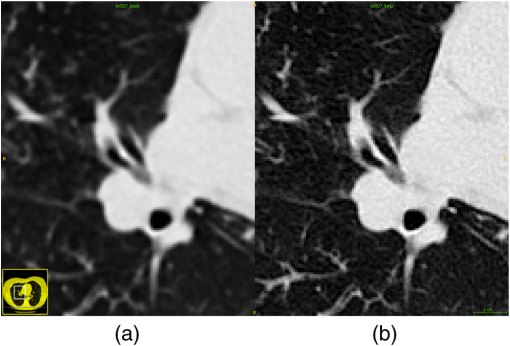 Table 3The images used for the reconstruction kernel experiment. This table lists which reconstruction kernel was used to generate the airways segmentation and distal point labeling. The make, model, and voxels size of the images are displayed in Table 1.
3.3.Biological Factors3.3.1.Effect of bifurcationsWe analyzed the effect of airway bifurcations on the tapering measurement. To this end, we manually identified regions of bifurcating airways. On a selected subset of airways, we considered the reconstructed airway image described in Fig. 16. Using ITK-SNAP, the author (K. Q.) started at the cross-sectional plane corresponding to the carina and scrolled toward the distal point. Using visual inspection, the following protocol was developed to identify bifurcations on cross-sectional planes:
Fig. 4(a) A region of bifurcation along the reconstructed slices. The green, blue, and red regions are the slices corresponding to the enlargement, break, and separation slices, respectively. The labeled region consists of slices from green to red. (b) A cross-sectional plane where the airway is at the point of bifurcation, indicated by the blue arrow. (c) First slice of the bifurcation region. (d) The final slice of the bifurcation region. The slides are chronologically ordered with the protocol described in Sec. 3.3.1.  For our experiment, we selected 19 airways from Table 1. The data consisted of 11 healthy and 8 bronchiectatic airways. The entire analysis was performed on ITK-SNAP.. 3.3.2.ProgressionWe examined possible changes in tapering of airways in patients over time. In this experiment, we consider two sets of longitudinal scans. First, pairs of airways that were healthy on both baseline and follow up scans. Second, pairs of airways that were healthy on baseline scans and became bronchiectatic on follow up scans. For pairs of healthy airways, a trained radiologist (J. J.), manually identified 14 pairs of airways across 3 patients. The criteria were the airway track that must have a healthy appearance on both baseline and follow up scans. For the second population, the same radiologist manually identified 5 pairs of airways from a single patient P1. The scans were obtained from the University College London Hospital and acquired with written consent. The criteria for selection were airways that appear healthy on baseline scans and became bronchiectatic at the follow up scan, an example is displayed in Fig. 5. Details of the CT images are summarized in Tables 4 and 5. Fig. 5The same pair of airways from longitudinal scans: (a) initial healthy airway and (b) the same airway at the same location becoming bronchiectatic. 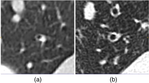 Using two separate work stations, the airways were visually registered between the longitudinal scans. Airways were taken from various regions of the lungs and were different to the airways displayed in Table 1. The tapering measurements were taken from the method discussed in Sec. 2. Table 4List of the images for progression experiment. This table includes time between scans in months (M) and days (D). The airways on this table are different to Table 1.
Table 5List of make, models, and voxel sizes of CT images for progression experiment. The voxel sizes are displayed as x, y, z and in mm units. Abbreviations: GEMS, GE medical systems; SS, Siemens SOMATOM.
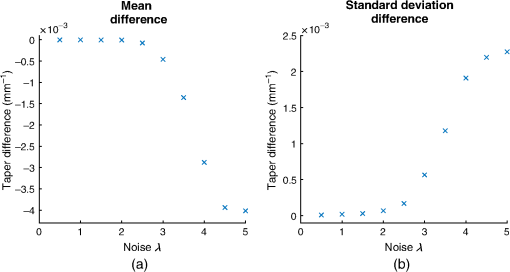
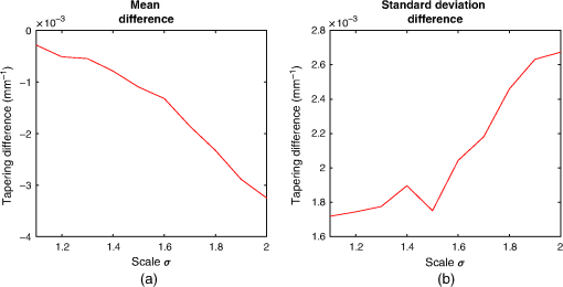
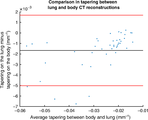
4.ResultsFigure 6 compares the tapering measurement between healthy and diseased airways. On a Wilcoxon rank-sum test between the populations, . Fig. 6Comparing the proposed tapering measurement with labeled healthy and bronchiectatic airways. On a Wilcoxon rank-sum test between the populations, . 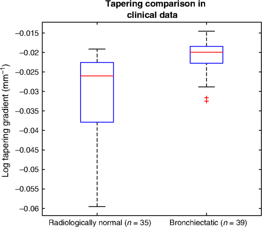 4.1.DoseWe analyzed the difference in cross-sectional area measurements and the final tapering measurements at different CT radiation doses. For the cross-sectional areas, Fig. 7 compares the cross-sectional areas between the original image and one of the noisy images. Each graph contains unique lumen measurements. The correlation coefficients between the populations were on all graphs. The 95% confidence intervals increase with the amount of noise. For the tapering measurement, Fig. 8 displays the measurements from all the noisy images compared to their respective original images. The correlation coefficient between noisy and original tapering measurements was on all values of . Fig. 7A series of Bland–Altman54 graphs comparing area measurements from a simulated low-dose scan and the original image. On all graphs, the correlation coefficient was . 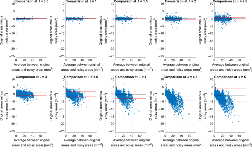 Fig. 8A series of Bland–Altman54 graphs comparing tapering measurement between simulated dose and the original image. On all graphs, the correlation coefficient was .  We analyzed the tapering difference between the original images and simulated images. We interpret the mean and standard deviation of the error difference as the bias and uncertainty, respectively. Figure 9 shows an overestimation bias with an increase in noise and a positive correlation between uncertainty and dose. 4.2.Voxel SizeWe analyzed the computed spline and tapering for all the scaled images. We used the arclength of the spline as the metric for comparison for the computed spline. Figure 10 compares the arclengths computed from the scaled splines with the respective originals. On all scales , the correlation coefficients between measurements were . Furthermore, we analyzed the error difference in arclength. In Fig. 11, the mean difference shows a weak correlation coefficient with with scale . The mean difference shows both an overestimation and underestimation bias with the arclength measurement. Figure 11 shows a weak correlation between standard deviation and scale with . Fig. 10A series of Bland–Altman54 graphs comparing arc lengths between scaled images and the original images. On all graphs, the correlation coefficient was . 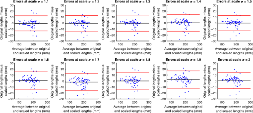 Fig. 11(a) Mean and (b) standard deviation of the difference in arclength between original images minus the scaled images. The correlation coefficient of the mean and standard deviation against scale are and , respectively. 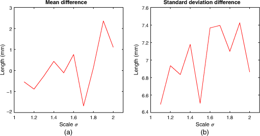 In terms of the tapering measurement, Fig. 12 compares the tapering values from the scaled images with the respective originals. The correlation coefficients between the scaled and original tapering values was on all scales . In addition, we examined the error difference of the original minus the scaled tapering. Figure 13 shows a negative correlation with both overestimation and scale with . Furthermore, Fig. 13 shows a positive correlation with uncertainty and scale with . Fig. 12A series of Bland–Altman54 graphs comparing tapering between original images and scaled images. On all graphs, the correlation coefficient was . 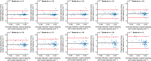 4.3.CT ReconstructionWe analyzed the difference in cross-sectional area and tapering measurement between reconstruction kernel. Figure 14, compares the difference in area measurements. On all patients, in cross-sectional area measurements, the correlation coefficient between the two measurements was . The largest 95% confidence was in patient bx515 with from the mean. Figure 15 compares the differences in tapering measurement. We collected tapering measurement from 4 patients. The correlation coefficient was between the reconstruction kernels. Fig. 14Bland–Altman54 graphs comparing the cross-sectional area between the lung and body kernels. On all four images, the correlation coefficient was . 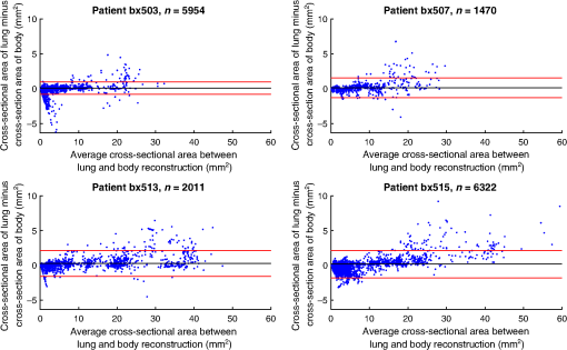 4.4.Clinical Results4.4.1.BifurcationsWe compared tapering measurements with and without points corresponding to bifurcations. On the first dataset, the tapering measurements were computed using all area measurements. The second dataset had tapering measurements computed without area measurements from the bifurcating regions as described in Fig. 16. As we compared the measurements in Fig. 17, the correlation coefficient was . Fig. 16(a) A signal of area measurement with bifurcation regions (red) and tubular regions (blue). (b) The same signal with tubular regions (blue) only. On both graphs, the black line is the linear regression of the respective data. The gradient of the line is the proposed tapering measurement. (c) The reconstructed bronchiectatic airway of the same profile. The blue-shaded and red-shaded regions correspond to the tubular and bifurcating airways, respectively. A reconstructed healthy airway has been discussed by Quan et al.27 Similar reconstructed cross-sectional images of vessels have been discussed by Oguma et al.,13 Kumar et al.,51 Alverez et al.,52 and Kirby et al.53 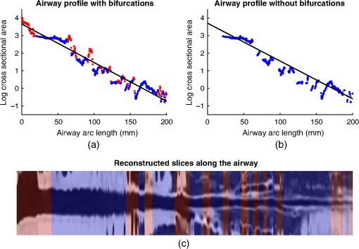 Fig. 17(a) Bland–Altman54 graph showing the relationship of the taper rates with and without bifurcations and (b) comparison of the standard error from linear regression between airways with and without bifurcations. On a Wilcoxon rank-sum test between the two populations, . 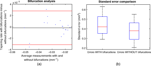 The uncertainty of each tapering measurement was computed using the standard error of estimate defined as55 where is the arclength, is the estimate from the linear regression from each computed area , and is the number of points in the profile. Figure 16 compares the uncertainty between the two populations. There was a statistical difference between the populations, on a Wilcoxon rank-sum test, .4.4.2.ProgressionFor healthy airways, we grouped tapering values between the baseline and follow up point. Figure 18 compares the measurements between the two time points. The results demonstrated good agreement with an intraclass correlation coefficient56 . The standard deviation of the tapering difference was . Fig. 18(a) Bland–Altman54 graph comparing tapering measurement on the same airways from the first and subsequent scan and (b) The change in tapering between healthy airways (H to H) and airways that became bronchiectatic on the follow up scans (H to D), . 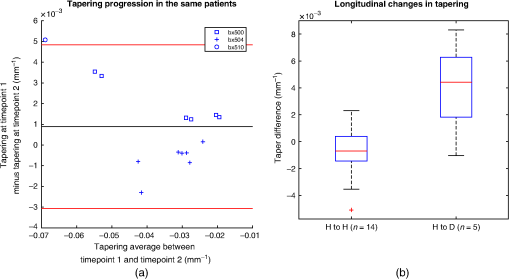 For airways that became bronchiectatic, we considered the change in tapering, i.e., tapering value at follow up minus tapering value at baseline, the results are displayed in Fig. 18. The results show that bronchiectatic airways have a greater tapering change in magnitude compared to airways that remained healthy . 5.DiscussionsIn this paper, we propose a tapering measurement for airways imaged using CT and validate the reproducibility of the measurement. The tapering measurement is the exponential decay constant between cross-sectional area and arclength from the carina to the distal point of the airway. Unlike other proposed tapering measurements, we assess reproducibility of the tapering measurement against simulated CT dose, voxel size, and CT reconstruction kernel. Finally, we assess the effect of tapering across airway bifurcations and examine repeatability over time using longitudinal scans. Part of the evaluations consists of analyzing the difference in tapering across longitudinal scans. The timescales between scans range from 9 to 35 months. The motivation for a long timescale is a proof of principle demonstration that the tapering measurement is reproducible for clinical studies. Examples include drug trails57 and investigations in exacerbations,58 where the timescales in monitoring patients were 12 months and 60 months, respectively. The pipeline consists of various established image processing algorithms. We chose the centerline algorithm developed by Palágyi et al.26 Unlike other proposed methods,30,59,60 the algorithm explicitly links the distal points to the carina. Furthermore, it has been shown that the algorithm of Palágyi et al.26 can be used on images with nonisotropic voxel sizes. By modeling the centerline as a graphical model similar to Mori et al.,31 we performed a breadth first search32 to avoid analyses of false airway branches. The removal of false branches is not a trivial task. 31,34,61 We corrected the centerline discretization error or recentering by smoothing points on the centerline. Smoothing has been an established method in the literature.34,62 A recentering method was proposed by Kiraly et al.,61 which shifts the centerline voxels in relation to a distance transform. The process is iterative compared to a single computation of smoothing. For our pipeline, we generated the orthonormal plane based on the method of Shirley and Marschner.38 We set the pixel size isotopically at 0.3 mm to insure that plane image to be within the resolution of the CT image and to allow the ray casting algorithm to find the lumen at subvoxel precision. Other methods have been proposed. In Ref. 36, Kreyszig generated a binormal and principle normal. However, the method is not robust as the binormal vector can become a zero vector. Grélard et al.63 used Voronoi cells, a method that requires two parameters whereas Shirley and Marschner38 is parameter free. For our work, intensities on the cross-sectional plane were computed via cubic interpolation. Various papers have used linear interpolation.39,64,65 However, it has been shown by Moses et al.66 that the method can create high-frequency artefacts in the image.67 Various methods have been proposed to measure the area of the airway lumen.68–70 We used the because of two distinct advantages. First, the method is parameter free. Second, the method is robust against slight variations in intensities. The method can, therefore, be applied to images from different scanners and images acquired using different image reconstruction kernels. 5.1.LimitationsIn this study, we compared the tapering measurement for healthy and diseased airways using a Wilcoxon rank-sum test. The test assumes the data points are independent. However, we used a variety of airways from the same lung. Thus the tapering profiles of the same patients will have a degree of overlap. Future work is needed to analyze data points that are not dependent on each other. A key limitation of the tapering measurement is the requirement of having a robust airway segmentation. In this paper, the airway segmentation software was often unable to reach the visible distal point of an airway. Thus time-consuming manual delineation was needed to extend the missing airways. The distal point is usually located at the periphery of the lungs. Thus to avoid manual labeling, a segmentation algorithm would need to automatically segment the airways past the sixth airway generation. From the literature, the state-of-the art software developed by Charbonnier et al.71 using deep learning could still only consistently segment airways to the fourth generation. The segmentation of small and peripheral airways is not a trivial task.66,72,73 In this paper, we analyze the reproducibility of all computerized components of the tapering algorithm. This paper does not address reproducibility of manual labeling of the airways. It is noted in the literature that semimanual labeling of small airways can take hours.74 Future work is required to analyze the reproducibility of manual segmentation of the airways. We hypothesize that the segmented healthy peripheral airways consist of a small number of voxels; therefore, any errors in voxel labeling will be considerably smaller then a dilated peripheral airway affected by bronchiectasis. In this work, we simulated low-dose scans through performing Radon transforms on existing CT images, adding Gaussian noise on the sinogram and using backprojection to reconstruct noisy CT images. There are proposed methods to simulate a low-dose scans by adding a combination of tailored Gaussian and Poisson noise on the sinogram.75 These methods assume the original high-dose sinogram are available for simulation; however, it has been acknowledged that sinograms are generally not available in the medical imaging community.76,77 Thus various groups have proposed low-dose simulations using reconstructed CT images. The methods involve adding Gaussian76,77 or a combination of Gaussian and Poisson noise78 on the sinogram of the forward projection of the CT image. Although there has been limited validation of the appearance of lung nodules against simulated low dose simulation,79 there has been no validation on the efficacy of these methods on the appearance of airways. We believe that our low-dose simulation is sufficient because the measured standard deviation of the trachea mask is similar to results taken from low-dose scans from Reeves et al.45 and Sui et al.47 Similarly, with voxel size simulation, ideally one would reconstruct the images from the original sinogram.19 However, as the sinograms were unavailable, we simulated the voxel size through interpolation of the original CT images similar to Robins et al.80 We believe that the simulation is sufficient as it shows the robustness and precision of the centerline, recentering, and cross-sectional plane algorithms in the pipeline. Changes in voxel sizes will change the combinatorics or arrangement of the binary image. By showing steps in the pipeline like centerline computation are repeatable across voxel sizes, we avoid resampling the image to isotropic lengths. Thus potentially avoiding a computationally expensive48 preprocessing step. We showed that the tapering measurement is reproducible by measuring the same airway across longitudinal scans with a minimum 5-month interval. The time between scans was on a similar scale from a reproducibility study on airway lumen by Brown et al.23 An ideal experiment to assess reproducibility of the same airway from different scans would be to acquire follow up scans immediately after baseline scans similar to Hammond et al.16 However, that work was performed on porcine models. Due to considerations of radiation dose, it is difficult to justify the acquisition of additional scans of no clinical benefit.81 For our experiment, each airway was chosen by a subspecialist thoracic radiologist. The airway was inspected to ensure it was in a healthy state, e.g., with no mucus present. Thus we assume that each pair of airways is disease free and healthy. 6.ConclusionsIn this paper, we show a statistical difference in tapering between healthy airways and those affected by bronchiectasis as judged by an experienced radiologist. From Fig. 6, the difference between the mean and median of the two populations was 0.011 and , respectively. In simulated low-dose scans, the tapering measurement retained a 95% confidence interval of up to , equivalent to a 25-mAs low-dose scan. In simulations assessing different voxel sizes, the tapering measurement retained a 95% confidence between up to . The tapering measurement retains the same 95% confidence, interval against variations in CT reconstruction kernels, bifurcations, and, importantly, over time in evaluating sequential scans in normal airways. Importantly, we showed as a proof of principle that the magnitude change in tapering for healthy airways is smaller than those from airways that became bronchiectatic. From our previous work,27 we showed that the measurements are accurate to a subvoxel level. Our findings suggest that our airway tapering measure can be used to assist in the diagnosis of bronchiectasis, to assess the progression of bronchiectasis with time and, potentially, to assess responses to therapy. We analyzed the reproducibility of the components that constitute the tapering measurements. The reproducibility of area measurements was analyzed in relation to simulated radiation dose and CT reconstruction kernels. For simulated dose, we found the 95% confidence interval retains in noisy images under , equivalent to a dose just higher than a 25-mAs low-dose scan. We note in Fig. 7, there is a bias toward overestimating larger lumen sizes at lower doses. As the centerline length remains constant and bias on the smaller lumen remain stable, the overestimation results in an increase in taper magnitude. For reconstruction kernels variation, we found the largest 95% confidence interval was . The reproducibly of arclengths was tested against voxel sizes variability and showed that arclengths have a 95% confidence interval of up to for scales under . The increase in the standard deviation of arclength and area against voxel size and dose, respectively, correlate with uncertainty in tapering. This paper provides useful information for clinical practice and clinical trials. An accurate prediction of the noise amplitude in a particular CT scan and its distribution is a function of the limited radiation dose of the scan, scanner geometry, reconstructed voxel size, other sources of noise, the reconstruction algorithm, and any pre- and postprocessing used. Many of these factors are proprietary information of the CT manufacturer and hence not available to users.82,83 We have undertaken an experiment to assess the dependence of our measurements on a simulated noise field added to the CT scan data and have presented the results. This gives an indication of the dependence on radiation dose assuming all other factors remain the same. We recommend that the accuracy experiment presented in this paper be repeated for the particular reconstruction, scan protocol, and scanner type used to make the measurements. Bronchiectasis is often described as an orphan disease and has suffered a lack of interest and funding.84,85 We have shown that the reproducibility of automated airway tapering measurements can assist in the diagnosis and management of bronchiectasis. In addition, we show that it is feasible to use our tapering measurement in large-scale clinical studies of the disease provided careful phantom calibration is taken. DisclosuresPart of this work has been presented at the 2018 SPIE Medical Imaging Conference.27 For potential conflicts of interest: Ryutaro Tanno has been employed by Microsoft, ThinkSono, and Butterfly Network (the employment is unrelated to the submitted work), Joseph Jacob has received fees from Boehringer Ingelheim and Roche (unrelated to the submitted work), and David Hawkes is a Founder Shareholder in Ixico plc (unrelated to the submitted work). The other authors have no conflicts of interest to declare. AcknowledgmentsKin Quan would like to thank Prof Simon Arridge and Dr Andreas Hauptmann for their helpful conversations on the low-dose simulations. This work is supported by the EPSRC-funded UCL Center for Doctoral Training in Medical Imaging (No. EP/L016478/1) and the Department of Health NIHR-funded Biomedical Research Center at the University College London Hospitals. Ryutaro Tanno is supported by Microsoft Research Scholarship. Joseph Jacob is a recipient of Wellcome Trust Clinical Research Career Development Fellowship No. 209553/Z/17/Z. ReferencesJ. D. Chalmers,
“Bronchiectasis exacerbations are heart-breaking,”
Ann. Am. Thorac. Soc., 15
(3), 301
–303
(2018). https://doi.org/10.1513/AnnalsATS.201710-832ED Google Scholar
M. C. Pasteur, D. Bilton and A. T. Hill,
“British thoracic society guideline for non-CF bronchiectasis,”
Thorax, 65 i1
–i58
(2010). https://doi.org/10.1136/thx.2010.136119 THORA7 0040-6376 Google Scholar
C. Fetita et al.,
“Grading remodeling severity in asthma based on airway wall thickening index and bronchoarterial ratio measured with MSCT,”
Proc. SPIE, 9415 941515
(2015). https://doi.org/10.1117/12.2081589 PSISDG 0277-786X Google Scholar
E. Ü. Mumcuoglu et al.,
“Image analysis for cystic fibrosis: computer-assisted airway wall and vessel measurements from low-dose, limited scan lung CT images,”
J. Digital Imaging, 26 82
–96
(2013). https://doi.org/10.1007/s10278-012-9476-4 JDIMEW Google Scholar
A. Perez-Rovira et al.,
“Automatic airway–artery analysis on lung CT to quantify airway wall thickening and bronchiectasis,”
Med. Phys., 43
(10), 5736
–5744
(2016). https://doi.org/10.1118/1.4963214 MPHYA6 0094-2405 Google Scholar
D. M. Hansell,
“Thin-section CT of the lungs: the Hinterland of normal,”
Radiology, 256
(3), 695
–711
(2010). https://doi.org/10.1148/radiol.10092307 RADLAX 0033-8419 Google Scholar
J. S. Kim et al.,
“Bronchoarterial ratio on thin section CT: comparison between high altitude and sea level,”
J. Comput. Assisted Tomogr., 21
(2), 306
–311
(1997). https://doi.org/10.1097/00004728-199703000-00028 JCATD5 0363-8715 Google Scholar
S. Matsuoka et al.,
“Bronchoarterial ratio and bronchial wall thickness on high-resolution CT in asymptomatic subjects: correlation with age and smoking,”
Am. J. Roentgenol., 180
(2), 513
–518
(2003). https://doi.org/10.2214/ajr.180.2.1800513 AJROAM 0092-5381 Google Scholar
A. A. Diaz et al.,
“Quantitative CT measures of bronchiectasis in smokers,”
Chest, 151
(6), 1255
–1262
(2017). https://doi.org/10.1016/j.chest.2016.11.024 CHETBF 0012-3692 Google Scholar
V. Cheplygina et al.,
“Early experiences with crowdsourcing airway annotations in chest CT,”
in Int. Workshop Large-Scale Annotation of Biomed. Data and Expert Label Synth.,
(2016). https://doi.org/10.1007/978-3-319-46976-8_22 Google Scholar
B. L. Odry et al.,
“Automated airway evaluation system for multi-slice computed tomography using airway lumen diameter, airway wall thickness and broncho-arterial ratio,”
Proc. SPIE, 6143 61430Q
(2006). https://doi.org/10.1117/12.653796 PSISDG 0277-786X Google Scholar
R. Venkatraman et al.,
“Fully automated system for three-dimensional bronchial morphology analysis using volumetric multidetector computed tomography of the chest,”
J. Digital Imaging, 19
(2), 132
–139
(2006). https://doi.org/10.1007/s10278-005-9240-0 JDIMEW Google Scholar
T. Oguma et al.,
“Longitudinal shape irregularity of airway lumen assessed by CT in patients with bronchial asthma and COPD,”
Thorax, 70
(8), 719
–724
(2015). https://doi.org/10.1136/thoraxjnl-2014-206651 THORA7 0040-6376 Google Scholar
O. Weinheimer et al.,
“Fully automated lobe-based airway taper index calculation in a low dose MDCT CF study over 4 time-points,”
Proc. SPIE, 10133 101330U
(2017). https://doi.org/10.1117/12.2254387 PSISDG 0277-786X Google Scholar
J. D. Chalmers, S. Aliberti and F. Blasi,
“State of the art review: management of bronchiectasis in adults,”
Eur. Respir. J., 45
(5), 1446
–1462
(2015). https://doi.org/10.1183/09031936.00119114 Google Scholar
E. Hammond et al.,
“Comparison of low- and ultralow-dose computed tomography protocols for quantitative lung and airway assessment,”
Med. Phys., 44
(9), 4747
–4757
(2017). https://doi.org/10.1002/mp.12436 MPHYA6 0094-2405 Google Scholar
Y. Jia et al.,
“Quantitative analysis of airway tree in low-dose chest CT with a new model-based iterative reconstruction algorithm: comparison to adaptive statistical iterative reconstruction in routine-dose CT,”
Acad. Radiol., 25
(12), 1526
–1532
(2018). https://doi.org/10.1016/j.acra.2018.03.021 Google Scholar
P. Leutz-Schmidt et al.,
“Influence of exposure parameters and iterative reconstruction on automatic airway segmentation and analysis on MDCT—An ex vivo phantom study,”
PLoS One, 12
(8), e0182268
(2017). https://doi.org/10.1371/journal.pone.0182268 POLNCL 1932-6203 Google Scholar
T. Achenbach et al.,
“Influence of pixel size on quantification of airway wall thickness in computed tomography,”
J. Comput. Assisted Tomogr., 33
(5), 725
–730
(2009). https://doi.org/10.1097/RCT.0b013e318190699a JCATD5 0363-8715 Google Scholar
J. Ken Leader et al.,
“Quantification of airway morphometry: the effect of CT acquisition and reconstruction parameters,”
Proc. SPIE, 6511 65111R
(2007). https://doi.org/10.1117/12.709940 PSISDG 0277-786X Google Scholar
J. C. Wong et al.,
“The influence of reconstruction algorithm on the measurement of airway dimensions using computed tomography,”
Proc. SPIE, 6916 691615
(2008). https://doi.org/10.1117/12.769697 PSISDG 0277-786X Google Scholar
B. Zheng et al.,
“Automated detection and quantitative assessment of pulmonary airways depicted on CT images,”
Med. Phys., 34
(7), 2844
–2852
(2007). https://doi.org/10.1118/1.2742777 MPHYA6 0094-2405 Google Scholar
R. H. Brown et al.,
“Reproducibility of airway luminal size in asthma measured by HRCT,”
J. Appl. Physiol., 123
(4), 876
–883
(2017). https://doi.org/10.1152/japplphysiol.00307.2017 Google Scholar
L. Zhang et al.,
“Airway quantification using adaptive statistical iterative reconstruction-V on wide-detector low-dose CT: a validation study on lung specimen,”
Jpn. J. Radiol., 37
(5), 390
–398
(2019). https://doi.org/10.1007/s11604-019-00818-2 Google Scholar
C. Fetita et al.,
“Volumetric quantification of airway wall in CT via collision-free active surface model: application to asthma assessment,”
IEEE Trans. Image Process., 33
(7), 1512
–1526
(2014). https://doi.org/10.1109/TMI.2014.2316115 IIPRE4 1057-7149 Google Scholar
K. Palágyi et al.,
“Quantitative analysis of pulmonary airway tree structures,”
Comput. Biol. Med., 36
(9), 974
–996
(2006). https://doi.org/10.1016/j.compbiomed.2005.05.004 CBMDAW 0010-4825 Google Scholar
K. Quan et al.,
“Tapering analysis of airways with bronchiectasis,”
Proc. SPIE, 10574 105742G
(2018). https://doi.org/10.1117/12.2292306 PSISDG 0277-786X Google Scholar
P. A. Yushkevich et al.,
“User-guided 3D active contour segmentation of anatomical structures: Significantly improved efficiency and reliability,”
(2019) http://www.itksnap.org July ). 2019). Google Scholar
E. M. van Rikxoort, B. Wouter and B. Van Ginneken,
“Automatic segmentation of the airway tree from thoracic CT scans using a multi-threshold approach,”
in The First Int. Workshop Pulmonary Image Anal.,
(2009). Google Scholar
S. R. Aylward and E. Bullitt,
“Initialization, noise, singularities, and scale in height ridge traversal for tubular object centerline extraction,”
IEEE Trans. Med. Imaging, 21
(2), 61
–75
(2002). https://doi.org/10.1109/42.993126 ITMID4 0278-0062 Google Scholar
K. Mori et al.,
“Automated anatomical labeling of the bronchial branch and its application to the virtual bronchoscopy system,”
IEEE Trans. Med. Imaging, 19
(2), 103
–114
(2000). https://doi.org/10.1109/42.836370 ITMID4 0278-0062 Google Scholar
T. H. Cormen et al., Introduction to Algorithms, MIT Press, Cambridge
(2009). Google Scholar
F. Grélard et al.,
“New methods for the geometrical analysis of tubular organs,”
Med. Image Anal., 42 89
–101
(2017). https://doi.org/10.1016/j.media.2017.07.008 Google Scholar
B. J. Irving et al.,
“Computer assisted detection of abnormal airway variation in CT scans related to paediatric tuberculosis,”
Med. Image Anal., 18
(7), 963
–976
(2014). https://doi.org/10.1016/j.media.2014.05.007 Google Scholar
,“Natural” or periodic interpolating cubic spline curve—MATLAB,”
https://uk.mathworks.com/help/curvefit/cscvn.html Google Scholar
E. Kreyszig, Advanced Engineering Mathematics, John Wiley & Sons, New York
(1964). Google Scholar
S. J. Leon, Linear Algebra with Applications, Pearson Prentice Hall, Upper Saddle River, New Jersey
(2009). Google Scholar
P. Shirley and S. Marschner, Fundamentals of Computer Graphics, A K Peters, Natick, Massachusetts
(2009). Google Scholar
A. P. Kiraly et al.,
“Virtual bronchoscopy for quantitative airway analysis,”
Proc. SPIE, 5746 369
–383
(2005). https://doi.org/10.1117/12.595283 PSISDG 0277-786X Google Scholar
A. W. Fitzgibbon, M. Pilu and R. B. Fisher,
“Direct least squares fitting of ellipses,”
in Proc. 13th Int. Conf. Pattern Recognit.,
(1996). https://doi.org/10.1109/ICPR.1996.546029 Google Scholar
A. I. Nikiforov and R. B. Schlesinger,
“Morphometric variability of the human upper bronchial tree,”
Respir. Physiol., 59
(3), 289
–299
(1985). https://doi.org/10.1016/0034-5687(85)90134-3 RSPYAK 0034-5687 Google Scholar
M. K. Azad, H. A. Mansy and P. T. Gamage,
“Geometric features of pig airways using computed tomography,”
Physiol. Rep., 4
(20), e12995
(2016). https://doi.org/10.14814/phy2.12995 Google Scholar
B. Milliron et al.,
“Bronchiectasis: mechanisms and imaging clues of associated common and uncommon diseases,”
RadioGraphics, 35
(4), 1011
–1030
(2015). https://doi.org/10.1148/rg.2015140214 Google Scholar
D. P. Frush et al.,
“Computer-simulated radiation dose reduction for abdominal multidetector CT of pediatric patients,”
Am. J. Roentgenol., 179
(2), 1107
–1113
(2002). https://doi.org/10.2214/ajr.179.5.1791107 AJROAM 0092-5381 Google Scholar
A. P. Reeves, Y. Xie and S. Liu,
“Automated image quality assessment for chest CT scans,”
Med. Phys., 45
(2), 561
–578
(2017). https://doi.org/10.1002/mp.12729 MPHYA6 0094-2405 Google Scholar
R. C. Gonzalez, R. E. Woods and S. L. Eddins, Digital Image Processing Using MATLAB, Pearson Prentice Hall, Upper Saddle River, New Jersey
(2011). Google Scholar
X. Sui et al.,
“Detection and size measurements of pulmonary nodules in ultra-low-dose CT with iterative reconstruction compared to low dose CT,”
Eur. J. Radiol., 85
(3), 564
–570
(2016). https://doi.org/10.1016/j.ejrad.2015.12.013 EJRADR 0720-048X Google Scholar
R. Wiemker et al.,
“Unsupervised extraction and quantification of the bronchial tree on ultra-low-dose vs. standard dose CT,”
Proc. SPIE, 6143 61432V
(2006). https://doi.org/10.1117/12.649530 PSISDG 0277-786X Google Scholar
A. Larbi et al.,
“Detection and characterization of focal liver lesions with ultra-low dose computed tomography in neoplastic patients,”
Diagn. Interventional Imaging, 99
(5), 311
–320
(2018). https://doi.org/10.1016/j.diii.2017.11.003 Google Scholar
Y. Nagatani et al.,
“Lung nodule detection performance in five observers on computed tomography (CT) with adaptive iterative dose reduction using three-dimensional processing (AIDR 3D) in a Japanese multicenter study: comparison between ultra-low-dose CT and low-dose CT by receiver-operating characteristic analysis,”
Eur. J. Radiol., 84
(7), 1401
–1412
(2015). https://doi.org/10.1016/j.ejrad.2015.03.012 EJRADR 0720-048X Google Scholar
R. P. Kumar et al.,
“Three-dimensional blood vessel segmentation and centerline extraction based on two-dimensional cross-section analysis,”
Ann. Biomed. Eng., 43
(5), 1223
–1234
(2015). https://doi.org/10.1007/s10439-014-1184-4 ABMECF 0090-6964 Google Scholar
L. Alvarez et al.,
“Tracking the aortic lumen geometry by optimizing the 3D orientation of its cross-sections,”
Lect. Notes Comput. Sci., 10434 174
–181
(2017). https://doi.org/10.1007/978-3-319-66185-8 LNCSD9 0302-9743 Google Scholar
M. Kirby et al.,
“Total airway count on computed tomography and the risk of chronic obstructive pulmonary disease progression,”
Am. J. Respir. Crit. Care Med., 197
(1), 56
–65
(2018). https://doi.org/10.1164/rccm.201704-0692OC AJCMED 1073-449X Google Scholar
J. M. Bland and D. G. Altman,
“Statistical methods for assessing agreement between two methods of clinical measurement,”
Lancet, 327
(8476), 307
–310
(1986). https://doi.org/10.1016/S0140-6736(86)90837-8 LANCAO 0140-6736 Google Scholar
M. R. Spiegal and L. J. Stephens, Schaum’s Outline of Theory and Problems of Statistics, McGraw-Hill Education, New York
(1998). Google Scholar
D. L. Streiner, G. R. Norman and J. Cariney, Health Measurement Scales: A Practical Guide to Their Development and Use, Oxford University Press, Oxford
(2015). Google Scholar
A. de Soyza et al.,
“RESPIRE 1: a phase III placebo-controlled randomised trial of ciprofloxacin dry powder for inhalation in non-cystic fibrosis bronchiectasis,”
Eur. Respir. J., 51 1702052
(2018). https://doi.org/10.1183/13993003.02052-2017 Google Scholar
J. D. Chalmers et al.,
“Characterization of the ‘frequent exacerbator phenotype’ in bronchiectasis,”
Am. J. Respir. Crit. Care Med., 197
(11), 1410
–1420
(2018). https://doi.org/10.1164/rccm.201711-2202OC AJCMED 1073-449X Google Scholar
R. Cardenes, H. Bogunovic and A. F. Frangi,
“Fast 3D centerline computation for tubular structures by front collapsing and fast marching,”
in IEEE Int. Conf. Image Process.,
(2010). https://doi.org/10.1109/ICIP.2010.5651609 Google Scholar
D. Jin et al.,
“A robust and efficient curve skeletonization algorithm for tree-like objects using minimum cost paths,”
Pattern Recognit. Lett., 76 32
–40
(2016). https://doi.org/10.1016/j.patrec.2015.04.002 PRLEDG 0167-8655 Google Scholar
A. P. Kiraly et al.,
“Three-dimensional path planning for virtual bronchoscopy,”
IEEE Trans. Med. Imaging, 23
(9), 1365
–1379
(2004). https://doi.org/10.1109/TMI.2004.829332 ITMID4 0278-0062 Google Scholar
Z. Xu et al.,
“A hybrid method for airway segmentation and automated measurement of bronchial wall thickness on CT,”
Med. Image Anal., 24
(1), 1
–17
(2015). https://doi.org/10.1016/j.media.2015.05.003 Google Scholar
F. Grélard et al.,
“Precise cross-section estimation on tubular organs,”
Lect. Notes Comput. Sci., 9257 277
–288
(2015). https://doi.org/10.1007/978-3-319-23117-4 LNCSD9 0302-9743 Google Scholar
B. L. Odry et al.,
“An evaluation of automated broncho-arterial ratios for reliable assessment of bronchiectasis,”
Proc. SPIE, 6915 69152M
(2008). https://doi.org/10.1117/12.772579 PSISDG 0277-786X Google Scholar
J. Tschirren et al.,
“Intrathoracic airway trees: segmentation and airway morphology analysis from low-dose CT scans,”
IEEE Trans. Med. Imaging, 24
(12), 1529
–1539
(2005). https://doi.org/10.1109/TMI.2005.857654 ITMID4 0278-0062 Google Scholar
D. A. Moses et al.,
“Peripheral bronchial identification on chest CT using unsupervised machine learning,”
Int. J. Comput. Assisted Radiol. Surg., 13
(9), 1379
–1395
(2018). https://doi.org/10.1007/s11548-018-1805-8 Google Scholar
P. Thévenaz, T. Blu and M. Unser,
“Interpolation revisited,”
IEEE Trans. Med. Imaging, 19
(7), 739
–758
(2000). https://doi.org/10.1109/42.875199 ITMID4 0278-0062 Google Scholar
S. Gu et al.,
“Computerized identification of airway wall in CT examinations using a 3D active surface evolution approach,”
Med. Image Anal., 17
(3), 283
–296
(2013). https://doi.org/10.1016/j.media.2012.11.003 Google Scholar
A. P. Kiraly et al.,
“Boundary-specific cost functions for quantitative airway analysis,”
Lect. Notes Comput. Sci., 4791 784
–791
(2007). https://doi.org/10.1007/978-3-540-75757-3 LNCSD9 0302-9743 Google Scholar
O. I. Saba, E. A. Hoffman and J. M. Reinhardt,
“Maximizing quantitative accuracy of lung airway lumen and wall measures obtained from X-ray CT imaging,”
J. Appl. Physiol., 95
(3), 1063
–1075
(2003). https://doi.org/10.1152/japplphysiol.00962.2002 Google Scholar
J.-P. Charbonnier et al.,
“Improving airway segmentation in computed tomography using leak detection with convolutional networks,”
Med. Image Anal., 36 52
–60
(2017). https://doi.org/10.1016/j.media.2016.11.001 Google Scholar
Z. Bian et al.,
“Small airway segmentation in thoracic computed tomography scans: A machine learning approach,”
Phys. Med. Biol., 63
(15), 155024
(2018). https://doi.org/10.1088/1361-6560/aad2a1 PHMBA7 0031-9155 Google Scholar
Z. Yang, H. Jin and J. H. Kim,
“Attenuation profile matching: an accurate and scan parameter-robust measurement method for small airway dimensions in low-dose CT scans,”
Med. Phys., 45
(9), 4145
–4157
(2018). https://doi.org/10.1002/mp.2018.45.issue-9 MPHYA6 0094-2405 Google Scholar
J. Tschirren, T. Yavarna and J. M. Reinhardt,
“Airway segmentation framework for clinical environments,”
in The Second Int. Workshop Pulmonary Image Anal.,
(2009). Google Scholar
S. Žabić et al.,
“A low dose simulation tool for CT systems with energy integrating detectors,”
Med. Phys., 40
(3), 031102
(2013). https://doi.org/10.1118/1.4789628 MPHYA6 0094-2405 Google Scholar
T. Takenaga et al.,
“A computer simulation method for low-dose CT images by use of real high-dose images: a phantom study,”
Radiol. Phys. Technol., 9
(1), 44
–52
(2016). https://doi.org/10.1007/s12194-015-0332-3 Google Scholar
K. C. Won and J. H. Kim,
“Realistic simulation of reduced-dose CT with noise modeling and sinogram synthesis using DICOM CT images,”
Med. Phys., 41
(1), 011901
(2014). https://doi.org/10.1118/1.4830431 MPHYA6 0094-2405 Google Scholar
R. E. Naziroglu et al.,
“Simulation of scanner- and patient-specific low-dose CT imaging from existing CT images,”
Phys. Med., 36 12
–23
(2017). https://doi.org/10.1016/j.ejmp.2017.02.009 Google Scholar
X. Li et al.,
“Pediatric MDCT: towards assessing the diagnostic influence of dose reduction on the detection of small lung nodules,”
Acad. Radiol., 16
(7), 872
–880
(2009). https://doi.org/10.1016/j.acra.2009.01.028 Google Scholar
M. Robins et al.,
“How reliable are texture measurements?,”
Proc. SPIE, 10573 105733W
(2018). https://doi.org/10.1117/12.2294591 PSISDG 0277-786X Google Scholar
P. P. Dendy and B. Heaton, Physics for Diagnostic Radiology, Taylor & Francis, Boca Raton
(1999). Google Scholar
D. G. Parr et al.,
“Influence of calibration on densitometric studies of emphysema progression using computed tomography,”
Am. J. Respir. Crit. Care Med., 170 883
–890
(2004). https://doi.org/10.1164/rccm.200403-326OC AJCMED 1073-449X Google Scholar
B. C. Stoel et al.,
“Quality control in longitudinal studies with computed tomographic densitometry of the lungs,”
Proc. Am. Thorac. Soc., 5
(9), 929
–933
(2008). https://doi.org/10.1513/pats.200804-039QC Google Scholar
J. D. Chalmers et al.,
“The bronchiectasis severity index an international derivation and validation study,”
Am. J. Respir. Crit. Care Med., 189
(5), 576
–585
(2014). https://doi.org/10.1164/rccm.201309-1575OC AJCMED 1073-449X Google Scholar
J. R. Hurst,
“Microbial dysbiosis in bronchiectasis,”
Lancet Respir. Med., 2
(12), 945
–947
(2014). https://doi.org/10.1016/S2213-2600(14)70223-1 Google Scholar
BiographyKin Quan received his MSc degree in mathematics from the University College London. He is a PhD student studying medical imaging at the University College London. His research concerns measuring and interpreting the geometry of airways in CT. Ryutaro Tanno received his BSc and MASt degrees in pure mathematics from the Imperial College London and University of Cambridge, respectively, and his MPhil degree in computational neuroscience from the University of Cambridge. He is a Microsoft research PhD scholar. His interests are designing methods that can cheaply and reliably enhance the quality of medical image data. He has worked as a researcher for Mircosoft, ThinkSono, and Butterfly Network. Rebecca J. Shipley received her first class honours master’s degree in mathematics, before completing her DPhil (PhD) working on multiscale mathematical models of blood flow and drug delivery in vascularized tissues. She is a reader in biomechanics at the University College London. Her research involves computational modeling in biology and healthcare with a focus on tissue engineering and cancer. Currently, she is a director of the UCL Institute of Healthcare Engineering. Jeremy S. Brown is an academic respiratory consultant with a subspecialty interest in lung infection. He trained in respiratory medicine in London alternating with Wellcome-funded laboratory research at Imperial College into respiratory pathogens. He has led a laboratory investigating respiratory pathogens at the University College London since 2003 and been a clinical consultant at the University College Hospitals with a special interest in patients with respiratory infection and bronchiectasis. Joseph Jacob trained as a radiologist at Kings College Hospital with subspecialist chest radiology training at Imperial College London where he completed his MD (research). His research interest is computer-based analysis of CT imaging in lung disease for which, in 2018, he was awarded a Wellcome Trust Clinical Research Career Development Fellowship. He is based at the Center for Medical Image Computing and the Respiratory Medicine Department of the University College London. John R. Hurst is a professor of respiratory medicine at the University College London. He has clinical and research interests in bronchiectasis and COPD. He qualified from the University of Edinburgh Medical School in 1997 and has worked at UCL since 2007. He has national and international roles with the American and British Thoracic, and European Respiratory Societies and in 2019 will become the editor in chief of the European Respiratory Monograph. David J. Hawkes received his BA degree in natural sciences (physics) in 1974 from Oxford and his MSc degree in radiolobiology from Birmingham in 1975. He is a professor of computational imaging science at UCL. His research interests are focused on both fundamental research in medical image computing and transfer of advanced computational imaging technologies across the whole spectrum of patient management from screening to diagnosis, therapy planning, image-guided interventions, and treatment monitoring. |
