[go: up one dir, main page]

Next Issue
Volume 8, April
Previous Issue
Volume 7, December


J. Manuf. Mater. Process., Volume 8, Issue 1 (February 2024) – 42 articles

Cover Story (view full-size image): 
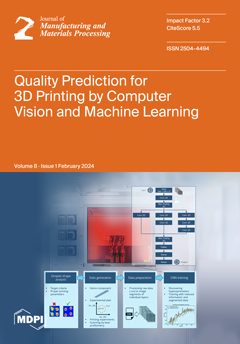
Multi-Material Jetting yields high precision in additive manufacturing of ceramics and metals, but it poses challenges in the choice of building strategies, as improper droplet overlap affects the process stability. The study addresses classification of process parameterization based on in-line surface measurements on green parts and processing with machine learning methods, in particular convolutional neural networks. Demo parts printed with different overlaps are scanned and labeled. Models with two convolutional layers and a pooling size of (6, 6) yield the best accuracies. Models trained only with images of the first layer obtained validation accuracies of 90%. Consequently, an arbitrary section of the first layer is sufficient to deliver a prediction about the quality of subsequently printed layers. View this paper
  • Issues are regarded as officially published after their release is announced to the table of contents alert mailing list.
  • You may sign up for e-mail alerts to receive table of contents of newly released issues.
  • PDF is the official format for papers published in both, html and pdf forms. To view the papers in pdf format, click on the "PDF Full-text" link, and use the free Adobe Reader to open them.
Order results
Result details
Select all
Export citation of selected articles as:
17 pages, 4514 KiB  
Article
Effect of Liquid Miscibility Gap on Defects in Inconel 625–GRCop42 Joints through Analysis of Gradient Composition Microstructure
by Jakub Preis, Donghua Xu, Brian K. Paul, Peter A. Eschbach and Somayeh Pasebani
J. Manuf. Mater. Process. 2024, 8(1), 42; https://doi.org/10.3390/jmmp8010042 - 14 Feb 2024
Cited by 4 | Viewed by 2062
Abstract
Joining of Cu-based dispersion-strengthened alloys to Ni-based superalloys has garnered increased attention for liquid rocket engine applications due to the high thermal conductivity of Cu-based alloys and high temperature tensile strength of Ni-based superalloys. However, such joints can suffer from cracking when joined [...] Read more.
Joining of Cu-based dispersion-strengthened alloys to Ni-based superalloys has garnered increased attention for liquid rocket engine applications due to the high thermal conductivity of Cu-based alloys and high temperature tensile strength of Ni-based superalloys. However, such joints can suffer from cracking when joined via liquid state processes, leading to part failure. In this work, compositions of 15–95 wt.% GRCop42 are alloyed with Inconel 625 and characterized to better understand the root cause of cracking. Results indicate a lack of miscibility between Cu-deprived and Cu-rich liquids in compositions corresponding to 30–95 wt.% GRCop42. Two distinct morphologies are observed and explained by use of CALPHAD; Cu-deprived dendrites with Cu-rich interdendritic zones at 30–50 wt.% GRCop42 and Cu-deprived spheres surrounded by a Cu-rich matrix at 60–95 wt.% GRCop42. Phase analysis reveals brittle intermetallic phases precipitate in the 60–95 wt.% GRCop42 Cu-deprived region. Three cracking mechanisms are proposed herein that provide guidance on the avoidance of defects Ni-based superalloy to Cu-based dispersion strengthened alloy joints. Full article
(This article belongs to the Special Issue Joining of Unweldable Materials: Concepts, Techniques and Processes)
Show Figures

Figure 1

Figure 1
<p>Optical micrographs of (<b>a</b>) 15 wt.% GRCop42, (<b>b</b>) cracking at the top of 30 wt.% GRCop42, (<b>c</b>) 50 wt.% GRCop42, (<b>d</b>) 60 wt.% GRCop42, (<b>e</b>) porosity 75 wt.% GRCop42, (<b>f</b>) cracking in 85 wt.% GRCop42, and (<b>g</b>) 95 wt.% GRCop42. For the etched samples (<b>c</b>,<b>d</b>,<b>g</b>), dark regions are Cu-rich while gray regions are Cu-deprived. The bold numbers at the top right of each micrograph correspond to the wt.% of GRCop42.</p>
Full article ">Figure 2
<p>SEM-EDS maps of (<b>a</b>) the Cu-rich region of the 75 wt.% GRCop42 sample and (<b>b</b>) the 50 wt.% GRCop42 sample. The bold number to the top right corresponds to the wt.% of GRCop42.</p>
Full article ">Figure 3
<p>XRD spectrum of (<b>a</b>) the 75 wt.% GRCop42 Cu-rich region and (<b>b</b>) 50 wt.% GRCop42. Both spectra show only FCC peaks.</p>
Full article ">Figure 4
<p>STEM-EDS maps showing the (<b>a</b>) HCP C14-Laves in the 85 wt.% GRCop42 Cu-deprived region along with (<b>b</b>) the corresponding SAD pattern in the [201] zone axis, (<b>c</b>) FCC NiNb<sub>5</sub> phase in the 95 wt.% GRCop42 Cu-deprived region along with (<b>d</b>) the corresponding SAD pattern in the [102] zone axis, and BCC <math display="inline"><semantics> <mi>α</mi> </semantics></math> Mo-Nb-Cr phase in the 95 wt.% GRCop42 Cu-deprived region with (<b>e</b>) the corresponding SAD pattern in the [314] zone axis. The arrows in (<b>a</b>,<b>c</b>,<b>e</b>) point to the location of SAD pattern collection. The circled spots in (<b>d</b>) are attributed to double diffraction.</p>
Full article ">Figure 5
<p>EBSD phase maps of the Cu-deprived region in the (<b>a</b>) 60, (<b>b</b>) 70, (<b>c</b>) 75, (<b>d</b>) 85, (<b>e</b>) 90, and (<b>f</b>) 95 wt.% GRCop42 samples. The bold number in the top left corner of each image corresponds to the wt.% of GRCop42. The table below each image shows the area fraction of the present phases. For (<b>e</b>,<b>f</b>) the area fraction is normalized to exclude the entrapped Cu FCC phase.</p>
Full article ">Figure 6
<p>Vickers microhardness of the Cu-deprived region and Cu-rich region from <a href="#jmmp-08-00042-t002" class="html-table">Table 2</a> and overlaid onto phase volume fractions from <a href="#jmmp-08-00042-f005" class="html-fig">Figure 5</a>.</p>
Full article ">Figure 7
<p>Equilibrium modeling of phase volume fractions as a function of (<b>a</b>) GRCop42 wt.% at each composition’s liquidus and as a function of temperature at (<b>b</b>) 30 wt.% GRCop42, (<b>c</b>) 50 wt.% GRCop42, and (<b>d</b>) 70 wt.% GRCop42. For (<b>a</b>), the estimated volume fraction of the Cu-deprived region from <a href="#jmmp-08-00042-t002" class="html-table">Table 2</a> was overlaid.</p>
Full article ">Figure 8
<p>Illustration of proposed miscibility gap failure mechanisms in Inconel 625–GRCop42 mixtures.</p>
Full article ">Figure A1
<p>CT scan of the 85 wt.% GRCop42 sample showing (<b>a</b>) a side view and (<b>b</b>) a top view. The dotted lines show corresponding view cutout locations. The light gray region corresponds to a Cu-deprived composition, while the dark gray region corresponds to a Cu-rich region.</p>
Full article ">
16 pages, 7266 KiB  
Article
Exploring New Parameters to Advance Surface Roughness Prediction in Grinding Processes for the Enhancement of Automated Machining
by Mohammadjafar Hadad, Samareh Attarsharghi, Mohsen Dehghanpour Abyaneh, Parviz Narimani, Javad Makarian, Alireza Saberi and Amir Alinaghizadeh
J. Manuf. Mater. Process. 2024, 8(1), 41; https://doi.org/10.3390/jmmp8010041 - 14 Feb 2024
Cited by 5 | Viewed by 2209
Abstract
Extensive research in smart manufacturing and industrial grinding has targeted the enhancement of surface roughness for diverse materials including Inconel alloy. Recent studies have concentrated on the development of neural networks, as a subcategory of machine learning techniques, to predict non-linear roughness behavior [...] Read more.
Extensive research in smart manufacturing and industrial grinding has targeted the enhancement of surface roughness for diverse materials including Inconel alloy. Recent studies have concentrated on the development of neural networks, as a subcategory of machine learning techniques, to predict non-linear roughness behavior in relation to various parameters. Nonetheless, this study introduces a novel set of parameters that have previously been unexplored, contributing to the advancement of surface roughness prediction for the grinding of Inconel 738 superalloy considering the effects of dressing and grinding parameters. Hence, the current study encompasses the utilization of a deep artificial neural network to forecast roughness. This implementation leverages an extensive dataset generated in a recent experimental study by the authors. The dataset comprises a multitude of process parameters across diverse conditions, including dressing techniques such as four-edge and single-edge diamond dresser, alongside cooling approaches like minimum quantity lubrication and conventional wet techniques. To evaluate a robust algorithm, a method is devised that involves different networks utilizing various activation functions and neuron sizes to distinguish and select the best architecture for this study. To gauge the accuracy of the methods, mean squared error and absolute accuracy metrics are applied, yielding predictions that fall within acceptable ranges for real-world industrial roughness standards. The model developed in this work has the potential to be integrated with the Industrial Internet of Things to further enhance automated machining. Full article
(This article belongs to the Special Issue Industry 4.0: Manufacturing and Materials Processing)
Show Figures

Figure 1

Figure 1
<p>A standard feedforward neural network structure with backpropagation error estimation. This is capable of learning and solving any nonlinear function, and, because of that, this network is popularly known as Universal Function Approximation [<a href="#B10-jmmp-08-00041" class="html-bibr">10</a>].</p>
Full article ">Figure 2
<p>Experimental setup: (a) grinding wheel, (b) coolant–lubricant nozzle, (c) dressing tool, (d) dressing table, and (e) dressing table controller.</p>
Full article ">Figure 3
<p>ANN implementation that contains one (<b>a</b>) and two hidden layers (<b>b</b>) with all properties that are included in the deep network.</p>
Full article ">Figure 4
<p>Data preparation, training, and testing.</p>
Full article ">Figure 5
<p>Workpiece surface roughness vs. dressing speed for dressing depth of 5 µm and single-edge dresser after (<b>a</b>) MQL grinding and (<b>b</b>) wet grinding [<a href="#B37-jmmp-08-00041" class="html-bibr">37</a>].</p>
Full article ">Figure 6
<p>Workpiece surface roughness vs. dressing speed for dressing depth of 10 µm and single-edge dresser after (<b>a</b>) MQL grinding and (<b>b</b>) wet grinding [<a href="#B37-jmmp-08-00041" class="html-bibr">37</a>].</p>
Full article ">Figure 7
<p>Workpiece surface roughness vs. dressing speed for a dressing depth of 5 µm and four-edge dresser after (<b>a</b>) MQL grinding and (<b>b</b>) wet grinding; and for a dressing depth of 10 µm and four-edge dresser after (<b>c</b>) MQL grinding and (<b>d</b>) wet grinding. [<a href="#B37-jmmp-08-00041" class="html-bibr">37</a>].</p>
Full article ">Figure 8
<p>The figure above presents the outcomes of various network implementations. Two network structures were employed, featuring either one hidden layer or two hidden layers. Each hidden layer utilized activation functions such as tansig and logsig, along with varying neuron quantities. The figure showcases the relationship between neuron quantity and Mean Squared Error (MSE), serving as an accuracy metric for the implemented networks.</p>
Full article ">Figure 9
<p>Predicted versus Real date for: (<b>a</b>) RT, (<b>b</b>) GPR, and (<b>c</b>) ANN.</p>
Full article ">Figure A1
<p>Comparison of the real surface roughness (R<sub>z</sub>) against predicted roughness with ANN (<b>a</b>). It is noteworthy to observe that the predicted observations from the test data closely match the ideal prediction in (<b>b</b>).</p>
Full article ">
42 pages, 11611 KiB  
Review
Negative Thermal Expansion Metamaterials: A Review of Design, Fabrication, and Applications
by Devashish Dubey, Anooshe Sadat Mirhakimi and Mohamed A. Elbestawi
J. Manuf. Mater. Process. 2024, 8(1), 40; https://doi.org/10.3390/jmmp8010040 - 14 Feb 2024
Cited by 5 | Viewed by 4228
Abstract
Most materials conventionally found in nature expand with an increase in temperature. In actual systems and assemblies like precision instruments, this can cause thermal distortions which can be difficult to handle. Materials with a tendency to shrink with an increase in temperature can [...] Read more.
Most materials conventionally found in nature expand with an increase in temperature. In actual systems and assemblies like precision instruments, this can cause thermal distortions which can be difficult to handle. Materials with a tendency to shrink with an increase in temperature can be used alongside conventional materials to restrict the overall dimensional change of structures. Such structures, also called negative-thermal-expansion materials, could be crucial in applications like electronics, biomedicine, aerospace components, etc., which undergo high changes in temperature. This can be achieved using mechanically engineered materials, also called negative thermal expansion (NTE) mechanical metamaterials. Mechanical metamaterials are mechanically architected materials with novel properties that are rare in naturally occurring materials. NTE metamaterials utilize their artificially engineered architecture to attain the rare property of negative thermal expansion. The emergence of additive manufacturing has enabled the feasible production of their intricate architectures. Industrial processes such as laser powder bed fusion and direct energy deposition, both utilized in metal additive manufacturing, have proven successful in creating complex structures like lattice formations and multimaterial components in the industrial sector, rendering them suitable for manufacturing NTE structures. Nevertheless, this review examines a range of fabrication methods, encompassing both additive and traditional techniques, and explores the diverse materials used in the process. Despite NTE metamaterials being a prominent field of research, a comprehensive review of these architected materials is missing in the literature. This article aims to bridge this gap by providing a state-of-the-art review of these metamaterials, encompassing their design, fabrication, and cutting-edge applications. Full article
(This article belongs to the Topic Additive Manufacturing of Architected Metallic Materials)
Show Figures

Figure 1

Figure 1
<p>2D NTE metamaterials: (<b>A</b>) Bimaterial-strip-based: (a) Concept of bimaterial strip (Reprinted with permission from [<a href="#B12-jmmp-08-00040" class="html-bibr">12</a>]; Copyright 1996 Springer Nature), (b) Cellular structure of bimaterial strips (Reprinted with permission from [<a href="#B12-jmmp-08-00040" class="html-bibr">12</a>]; Copyright Springer Nature), and (c) Equilateral triangular lattice using curved bimaterial ribs [<a href="#B14-jmmp-08-00040" class="html-bibr">14</a>]. (<b>B</b>) Multilayered strip with vertical NTE (Reprinted with permission from [<a href="#B19-jmmp-08-00040" class="html-bibr">19</a>]; Copyright 2010 John Wiley and Sons.). (<b>C</b>) Chirality-based: (a) Chiral lattice with bimaterial strip ligaments where lighter blue and darker blue represent two different constituents (Reprinted with permission from [<a href="#B16-jmmp-08-00040" class="html-bibr">16</a>]; Copyright 2015 John Wiley and sons), and (b) Bimaterial anti-tetrachiral and anti-trichiral lattice units (Reprinted with permission from [<a href="#B20-jmmp-08-00040" class="html-bibr">20</a>]; Copyright 2016 American Chemical Society). (<b>D</b>) Stretch-based: (a) Triangular grid design (Reprinted with permission from [<a href="#B17-jmmp-08-00040" class="html-bibr">17</a>]; Copyright 2007 The Royal Society (U.K.)), (b) Triangle lattice NTE (Reprinted with permission from [<a href="#B21-jmmp-08-00040" class="html-bibr">21</a>]; Copyright 2007 Elsevier), and (c) Hexagonal lattice design (Reprinted with permission from [<a href="#B22-jmmp-08-00040" class="html-bibr">22</a>]; Copyright 2016 Elsevier). (<b>E</b>) Others NTE designs: (a) Hoberman-circle-inspired design where red colour represents the constituent with larger CTE while blue represents constituent with lower CTE (Reprinted with permission from [<a href="#B23-jmmp-08-00040" class="html-bibr">23</a>]; Copyright 2018 Elsevier), (b) Hexagonal grid design (Reprinted with permission from [<a href="#B24-jmmp-08-00040" class="html-bibr">24</a>]; Copyright 2009 Elsevier), (c) Re-entrant structure where red colour represents the constituent with larger CTE while blue represents constituent with lower CTE (Reprinted with permission from [<a href="#B26-jmmp-08-00040" class="html-bibr">26</a>]; Copyright 2017 Elsevier), and (d) X-shaped structure (Reprinted with permission from [<a href="#B37-jmmp-08-00040" class="html-bibr">37</a>]; Copyright 2005 Springer Nature).</p>
Full article ">Figure 2
<p>3D NTE Metamaterials: (<b>a</b>) Tetrakaidecahedral foam cell with bimaterial strips (Reprinted with permission from [<a href="#B13-jmmp-08-00040" class="html-bibr">13</a>]; Copyright AIP Publishing), (<b>b</b>) Negative-CTE tetrahedron with material <span class="html-italic">a</span> having a low CTE and material <span class="html-italic">b</span> having a higher CTE (Reprinted with permission from [<a href="#B29-jmmp-08-00040" class="html-bibr">29</a>]; Copyright 2007 AIP Publishing), (<b>c</b>) Cubic quarter octahedral structure (Reprinted with permission from [<a href="#B32-jmmp-08-00040" class="html-bibr">32</a>]; Copyright 2017 Elsevier), (<b>d</b>) Anti-chiral 3D NTE structures (Reprinted with permission from [<a href="#B20-jmmp-08-00040" class="html-bibr">20</a>]; Copyright 2016 ACS Publications), (<b>e</b>) Star-shaped structures based on 2D re-entrant designs [<a href="#B25-jmmp-08-00040" class="html-bibr">25</a>]; Copyright 2018 Elsevier), and (<b>f</b>) Auxetic NTE structures (Reprinted with permission from [<a href="#B34-jmmp-08-00040" class="html-bibr">34</a>]; Copyright 2021 Elsevier).</p>
Full article ">Figure 3
<p>Comparison of powder bed fusion and direct energy deposition processes.</p>
Full article ">Figure 4
<p>Laser powder bed fusion setup schematic.</p>
Full article ">Figure 5
<p>Critical parameters in laser powder bed fusion.</p>
Full article ">Figure 6
<p>Multimaterial combinations fabricated using LPBF in research. The direction of arrows shows the order of fabrication of the parts (Information obtained from references [<a href="#B44-jmmp-08-00040" class="html-bibr">44</a>,<a href="#B45-jmmp-08-00040" class="html-bibr">45</a>,<a href="#B46-jmmp-08-00040" class="html-bibr">46</a>,<a href="#B47-jmmp-08-00040" class="html-bibr">47</a>,<a href="#B48-jmmp-08-00040" class="html-bibr">48</a>,<a href="#B49-jmmp-08-00040" class="html-bibr">49</a>,<a href="#B55-jmmp-08-00040" class="html-bibr">55</a>,<a href="#B56-jmmp-08-00040" class="html-bibr">56</a>,<a href="#B57-jmmp-08-00040" class="html-bibr">57</a>,<a href="#B58-jmmp-08-00040" class="html-bibr">58</a>,<a href="#B59-jmmp-08-00040" class="html-bibr">59</a>,<a href="#B60-jmmp-08-00040" class="html-bibr">60</a>,<a href="#B61-jmmp-08-00040" class="html-bibr">61</a>,<a href="#B62-jmmp-08-00040" class="html-bibr">62</a>]).</p>
Full article ">Figure 7
<p>(<b>a</b>) Powder-based and (<b>b</b>) wire-based DED setups.</p>
Full article ">Figure 8
<p>Critical parameters in direct energy deposition.</p>
Full article ">Figure 9
<p>Multimaterial combinations fabricated using DED in research. The direction of arrows shows the order of fabrication (Information obtained from references [<a href="#B49-jmmp-08-00040" class="html-bibr">49</a>,<a href="#B76-jmmp-08-00040" class="html-bibr">76</a>,<a href="#B79-jmmp-08-00040" class="html-bibr">79</a>,<a href="#B82-jmmp-08-00040" class="html-bibr">82</a>,<a href="#B83-jmmp-08-00040" class="html-bibr">83</a>,<a href="#B85-jmmp-08-00040" class="html-bibr">85</a>,<a href="#B86-jmmp-08-00040" class="html-bibr">86</a>,<a href="#B87-jmmp-08-00040" class="html-bibr">87</a>,<a href="#B91-jmmp-08-00040" class="html-bibr">91</a>,<a href="#B94-jmmp-08-00040" class="html-bibr">94</a>,<a href="#B95-jmmp-08-00040" class="html-bibr">95</a>,<a href="#B96-jmmp-08-00040" class="html-bibr">96</a>,<a href="#B97-jmmp-08-00040" class="html-bibr">97</a>,<a href="#B98-jmmp-08-00040" class="html-bibr">98</a>,<a href="#B99-jmmp-08-00040" class="html-bibr">99</a>,<a href="#B100-jmmp-08-00040" class="html-bibr">100</a>,<a href="#B101-jmmp-08-00040" class="html-bibr">101</a>,<a href="#B102-jmmp-08-00040" class="html-bibr">102</a>,<a href="#B103-jmmp-08-00040" class="html-bibr">103</a>,<a href="#B104-jmmp-08-00040" class="html-bibr">104</a>,<a href="#B105-jmmp-08-00040" class="html-bibr">105</a>,<a href="#B106-jmmp-08-00040" class="html-bibr">106</a>,<a href="#B107-jmmp-08-00040" class="html-bibr">107</a>,<a href="#B108-jmmp-08-00040" class="html-bibr">108</a>,<a href="#B109-jmmp-08-00040" class="html-bibr">109</a>,<a href="#B110-jmmp-08-00040" class="html-bibr">110</a>,<a href="#B111-jmmp-08-00040" class="html-bibr">111</a>,<a href="#B112-jmmp-08-00040" class="html-bibr">112</a>,<a href="#B113-jmmp-08-00040" class="html-bibr">113</a>,<a href="#B114-jmmp-08-00040" class="html-bibr">114</a>,<a href="#B115-jmmp-08-00040" class="html-bibr">115</a>,<a href="#B116-jmmp-08-00040" class="html-bibr">116</a>,<a href="#B117-jmmp-08-00040" class="html-bibr">117</a>,<a href="#B118-jmmp-08-00040" class="html-bibr">118</a>,<a href="#B119-jmmp-08-00040" class="html-bibr">119</a>,<a href="#B120-jmmp-08-00040" class="html-bibr">120</a>,<a href="#B121-jmmp-08-00040" class="html-bibr">121</a>,<a href="#B122-jmmp-08-00040" class="html-bibr">122</a>,<a href="#B123-jmmp-08-00040" class="html-bibr">123</a>,<a href="#B124-jmmp-08-00040" class="html-bibr">124</a>,<a href="#B125-jmmp-08-00040" class="html-bibr">125</a>,<a href="#B126-jmmp-08-00040" class="html-bibr">126</a>]).</p>
Full article ">Figure 10
<p>Schematic diagrams of various CM processes (Reprinted with permission from [<a href="#B179-jmmp-08-00040" class="html-bibr">179</a>]; Copyright 2020 Hasanov et al.).</p>
Full article ">Figure 11
<p>Electron backscatter diffraction (EBSD) maps of (<b>a</b>) LPBF-AlSi10Mg and (<b>b</b>) cast aluminium alloy. EBSD pole figures of (<b>c</b>) LPBF-AlSi10Mg and (<b>d</b>) cast aluminium alloy; (<b>e</b>) grain size area in LPBF-AlSi10Mg and the cast alloy (Reprinted with permission from [<a href="#B219-jmmp-08-00040" class="html-bibr">219</a>]; Copyright 2020 Elsevier).</p>
Full article ">Figure 12
<p>The iron–aluminium phase diagram (Reprinted with permission from [<a href="#B227-jmmp-08-00040" class="html-bibr">227</a>]; Copyright 1990 ASM International).</p>
Full article ">Figure 13
<p>The copper–nickel phase diagram (Reprinted with permission from [<a href="#B227-jmmp-08-00040" class="html-bibr">227</a>]; Copyright 1990 ASM International).</p>
Full article ">Figure 14
<p>CTE mismatch in electronic packaging.</p>
Full article ">Figure 15
<p>Young’s modulus and thermal expansion coefficient of semi-conductors and metals (data obtained from [<a href="#B238-jmmp-08-00040" class="html-bibr">238</a>,<a href="#B239-jmmp-08-00040" class="html-bibr">239</a>,<a href="#B240-jmmp-08-00040" class="html-bibr">240</a>]).</p>
Full article ">Figure 16
<p>Design of fuel cell (Reprinted with permission from [<a href="#B245-jmmp-08-00040" class="html-bibr">245</a>]; Copyright 2013 John Wiley and sons).</p>
Full article ">Figure 17
<p>Structure of a general dental implant (Reprinted with permission from [<a href="#B281-jmmp-08-00040" class="html-bibr">281</a>]; Copyright 2022 Elsevier).</p>
Full article ">Figure 18
<p>Fluctuating thermal environment in Earth’s orbit (Reprinted with permission from [<a href="#B295-jmmp-08-00040" class="html-bibr">295</a>]; Copyright 2023 Yu et al., Licensee MDPI).</p>
Full article ">Figure 19
<p>Negative expansion design by Milward et al. for cylindrical lens system meant for space applications (Reprinted with permission from [<a href="#B296-jmmp-08-00040" class="html-bibr">296</a>]; Copyright 2017 Milward et al.).</p>
Full article ">Figure 20
<p>Bimaterial hourglass hexagonal negative expansion design by Yu et al. (Reprinted with permission from [<a href="#B295-jmmp-08-00040" class="html-bibr">295</a>]; Copyright 2023 Yu et al., Licensee MDPI).</p>
Full article ">
13 pages, 12564 KiB  
Article
Fabrication of an Optically Transparent Planar Inverted-F Antenna Using PEDOT-Based Silver Nanowire Clear Ink with Aerosol-Jet Printing Method towards Effective Antennas
by Philip Li, Jason Fleischer, Edwin Quinn and Donghun Park
J. Manuf. Mater. Process. 2024, 8(1), 39; https://doi.org/10.3390/jmmp8010039 - 10 Feb 2024
Cited by 1 | Viewed by 1809
Abstract
We report the design, fabrication, and experimental characterization of an optically transparent printed planar inverted-F antenna (PIFA) operating at 2.45 GHz using the aerosol jet (AJ) printing method. The proposed antenna was fabricated using a clear conductive ink on glass and Delrin. The [...] Read more.
We report the design, fabrication, and experimental characterization of an optically transparent printed planar inverted-F antenna (PIFA) operating at 2.45 GHz using the aerosol jet (AJ) printing method. The proposed antenna was fabricated using a clear conductive ink on glass and Delrin. The antenna exhibits a wide fractional bandwidth (FBW) of 20% centered at 2.45 GHz, with a peak realized gain of −3.6 dBi and transparency of ~80%. The proposed fabrication method provides a cost-effective and scalable solution for manufacturing transparent antennas with potential applications in wireless communication, sensing, and wearable devices operating at mmWave frequencies higher than 30 GHz. Full article
Show Figures

Figure 1

Figure 1
<p>(<b>left</b>) Schematics of PIFA and (<b>right</b>) fabricated transparent PIFA on a glass substrate showing transparency.</p>
Full article ">Figure 2
<p>Photo overview of Optomec<sup>®</sup> AJ5X system with 5-axis trunnion. Additional modifications to the tool are pointed out in the figure.</p>
Full article ">Figure 3
<p>Sample traces made of clear ink. Note that both optical transparency and resistance decrease with increasing number of layers.</p>
Full article ">Figure 4
<p>Complex refractive index of typical ITOs. (<b>a</b>) Delta Technologies Product #: CB-40IN-0111 and (<b>b</b>) Thin Film Devices<sup>TM</sup> ITO. Note that the imaginary part of the refractive index decreases with a shorter wavelength. Both show a good transparency in the visible spectrum when the thickness is about a few μm.</p>
Full article ">Figure 5
<p>Estimated complex refractive index of CI (PEDOT:PSS + silver nanowire). The offset of 0.01 in the imaginary part of the complex refractive index was added to get a better agreement with the experimental data.</p>
Full article ">Figure 6
<p>Transmission test of CI (PEDOT:PSS + silver nanowire composite).</p>
Full article ">Figure 7
<p>Gain patterns of (<b>a</b>) CI/glass and (<b>b</b>) CI/Delrin samples.</p>
Full article ">Figure 8
<p>S11 on Smith Chart for CI/glass and CI/Delrin from 1.68 GHz to 3.12 GHz. The clear antenna on the Delrin substrate shows less reflection.</p>
Full article ">Figure 9
<p>Simulations of directivity (D), gain (G), and efficiency (e = G/D) of (<b>a</b>) CI/glass and (<b>b</b>) CI/Delrin samples.</p>
Full article ">Figure 10
<p>Reflection spectrums (<b>left</b>: simulation, <b>right</b>: experiment) of PIFAs on both glass (green) and Delrin (blue) substrates. Note that the experimental S11s of both samples show a good reflection spectrum, indicating ~1 GHz and ~0.85 GHz bandwidths for CI/glass and CI/Delrin samples, respectively.</p>
Full article ">Figure 11
<p>Measured gain patterns of (<b>top</b>) CI/glass and (<b>bottom</b>) DOWA/glass. Total Max: maximum gain, Max 3 db BW: 3 dB beam width, FSPL: Free Space Path Loss. We measured the gain of the antennas by exposing it to a frequency-swept RF signal from a source horn antenna. Then, we calculated its antenna’s gain using the substitution method.</p>
Full article ">Figure 12
<p>Printing multiple mmWave PIFAs on a glass substrate using AJ printing technique.</p>
Full article ">
14 pages, 4900 KiB  
Article
The Effect of Niobium Addition on the Operational and Metallurgical Behavior of Fe-Cr-C Hardfacing Deposited by Shielded Metal Arc Welding
by Jaime Perez, Jesus Gutierrez, Jhon Olaya, Oscar Piamba and Americo Scotti
J. Manuf. Mater. Process. 2024, 8(1), 38; https://doi.org/10.3390/jmmp8010038 - 10 Feb 2024
Cited by 1 | Viewed by 1772
Abstract
Hardfacing is commonly used in parts recovery and in obtaining surfaces with improved properties. Within this field, it is important to analyze the effect of alloying elements on the properties of the deposited layers. One of the critical parameters affecting alloying performances in [...] Read more.
Hardfacing is commonly used in parts recovery and in obtaining surfaces with improved properties. Within this field, it is important to analyze the effect of alloying elements on the properties of the deposited layers. One of the critical parameters affecting alloying performances in SMAW is improper arc length. This article examines the effect of the addition of niobium in different quantities (0, 2, 4, 6, and 8% by weight) to the electrode coating in Fe-Cr-C shielded metal arc welding (SMAW), with short and long arc lengths, on the operational process efficiency, dilution, arc energy, microstructure, and microhardness of the deposited layers. A decrease in operational process efficiency and dilution was found with increases in niobium content. On the other hand, it was found that adding niobium leads to a refinement in chromium carbide sizes, directly affecting the hardness of the obtained deposits. There is a direct relationship between the arc energy, with both short and long arc lengths, leading to a tendency to decrease the dilution in the obtained hardfacing. Full article
(This article belongs to the Special Issue Advances in Welding Technology)
Show Figures

Figure 1

Figure 1
<p>Cross-section schematic from hardfacing deposit.</p>
Full article ">Figure 2
<p>Electrode deposition efficiency as a function of the niobium content, where LA stands for long arc and SA for short arc.</p>
Full article ">Figure 3
<p>Arc energy as a function of niobium content in the electrode with two different arc lengths.</p>
Full article ">Figure 4
<p>Dilution in the bead-on-plate depositions as a function of the niobium content at 0, 2, 4, 6, and 8% (%weight) with short and long arcs.</p>
Full article ">Figure 5
<p>XRD pattern for coatings obtained using a short arc for the 5 electrode configurations.</p>
Full article ">Figure 6
<p>SEM images of the bead cross-section deposited with 0% niobium: (<b>a</b>) long arc; (<b>b</b>) short arc.</p>
Full article ">Figure 7
<p>SEM images of the bead cross-section deposited with 2% niobium: (<b>a</b>) long arc; (<b>b</b>) short arc.</p>
Full article ">Figure 8
<p>SEM images of the bead cross-section deposited with 4% niobium: (<b>a</b>) long arc; (<b>b</b>) short arc.</p>
Full article ">Figure 9
<p>SEM images of the bead cross-section deposited with 6% niobium: (<b>a</b>) long arc; (<b>b</b>) short arc.</p>
Full article ">Figure 10
<p>SEM images of the bead cross-section deposited with 8% niobium: (<b>a</b>) long arc; (<b>b</b>) short arc.</p>
Full article ">Figure 11
<p>Averages and standard deviations of microhardness for the beads obtained with different niobium content under long-arc (AL) and short-arc (AC) conditions.</p>
Full article ">Figure 12
<p>Chromium carbide sizes in the coatings obtained with different niobium content under long-arc (AL) and short-arc (AC) conditions.</p>
Full article ">Figure 13
<p>Niobium carbide sizes for coatings obtained with different niobium content under long-arc (LA) and short-arc (SA) conditions.</p>
Full article ">
46 pages, 12054 KiB  
Review
INCONEL® Alloy Machining and Tool Wear Finite Element Analysis Assessment: An Extended Review
by André F. V. Pedroso, Naiara P. V. Sebbe, Rúben D. F. S. Costa, Marta L. S. Barbosa, Rita C. M. Sales-Contini, Francisco J. G. Silva, Raul D. S. G. Campilho and Abílio M. P. de Jesus
J. Manuf. Mater. Process. 2024, 8(1), 37; https://doi.org/10.3390/jmmp8010037 - 9 Feb 2024
Cited by 3 | Viewed by 2184
Abstract
Machining INCONEL® presents significant challenges in predicting its behaviour, and a comprehensive experimental assessment of its machinability is costly and unsustainable. Design of Experiments (DOE) can be conducted non-destructively through Finite Element Analysis (FEA). However, it is crucial to ascertain whether numerical [...] Read more.
Machining INCONEL® presents significant challenges in predicting its behaviour, and a comprehensive experimental assessment of its machinability is costly and unsustainable. Design of Experiments (DOE) can be conducted non-destructively through Finite Element Analysis (FEA). However, it is crucial to ascertain whether numerical and constitutive models can accurately predict INCONEL® machining. Therefore, a comprehensive review of FEA machining strategies is presented to systematically summarise and analyse the advancements in INCONEL® milling, turning, and drilling simulations through FEA from 2013 to 2023. Additionally, non-conventional manufacturing simulations are addressed. This review highlights the most recent modelling digital solutions, prospects, and limitations that researchers have proposed when tackling INCONEL® FEA machining. The genesis of this paper is owed to articles and books from diverse sources. Conducting simulations of INCONEL® machining through FEA can significantly enhance experimental analyses with the proper choice of damage and failure criteria. This approach not only enables a more precise calibration of parameters but also improves temperature (T) prediction during the machining process, accurate Tool Wear (TW) quantity and typology forecasts, and accurate surface quality assessment by evaluating Surface Roughness (SR) and the surface stress state. Additionally, it aids in making informed choices regarding the potential use of tool coatings. Full article
Show Figures

Figure 1

Figure 1
<p>Subdivision of the JC constitutive model equation according to distinct deformation phenomena and the corresponding experimental trials and conditions [<a href="#B38-jmmp-08-00037" class="html-bibr">38</a>].</p>
Full article ">Figure 2
<p>Measured true-stress–strain (<span class="html-italic">σ<sub>tr</sub></span>-<span class="html-italic">ε<sub>tr</sub></span>) curves (discrete points) for (<b>a</b>) INCONEL<sup>®</sup> 718 and (<b>b</b>) INCONEL<sup>®</sup> 625. Corresponding computed results (solid lines) from the material model after calibration. The tests were performed with a nominal <math display="inline"><semantics> <mrow> <mover accent="true"> <mrow> <mi>ε</mi> </mrow> <mo>˙</mo> </mover> </mrow> </semantics></math> = 0.01 Hz for INCONEL<sup>®</sup> 625, while INCONEL<sup>®</sup> 718 was tested with 0.01 &lt; <math display="inline"><semantics> <mrow> <mover accent="true"> <mrow> <mi>ε</mi> </mrow> <mo>˙</mo> </mover> </mrow> </semantics></math> &lt; 1 Hz (adapted from [<a href="#B59-jmmp-08-00037" class="html-bibr">59</a>]).</p>
Full article ">Figure 3
<p>Standard uniaxial engineering <span class="html-italic">σ</span>-<span class="html-italic">ε</span> behaviour characteristic of a ductile material (adapted from [<a href="#B16-jmmp-08-00037" class="html-bibr">16</a>]).</p>
Full article ">Figure 4
<p>The development of chip morphology is impacted by prior machining operations, including (<b>a</b>) the influence of the initial chip thickness (<span class="html-italic">h</span><sub>ch</sub>), (<b>b</b>) the impact of the rake angle (<span class="html-italic">γ</span>) of the tool, (<b>c</b>) the ramifications of the tool’s edge radius (<span class="html-italic">r</span><sub>β</sub>), and (<b>d</b>) the effects of intervening cuts [<a href="#B60-jmmp-08-00037" class="html-bibr">60</a>].</p>
Full article ">Figure 5
<p>Procedure of Hosseinkhani and Ng’s [<a href="#B91-jmmp-08-00037" class="html-bibr">91</a>] proposed methodology.</p>
Full article ">Figure 6
<p>Orthogonal cutting model with a minimal width of cut (merely 4 μm) employing the CEL approach: (<b>a</b>) mesh structure and (<b>b</b>) specifications of boundary conditions [<a href="#B114-jmmp-08-00037" class="html-bibr">114</a>].</p>
Full article ">Figure 7
<p>Difference in numerical behaviour between the CEL and LAG approaches when studying <math display="inline"><semantics> <mrow> <msup> <mrow> <mover accent="true"> <mrow> <mi>ε</mi> </mrow> <mo>¯</mo> </mover> </mrow> <mrow> <mi>p</mi> </mrow> </msup> </mrow> </semantics></math> (<b>a</b>,<b>b</b>) and <span class="html-italic">T</span> (<b>c</b>,<b>d</b>). Cutting speed, <span class="html-italic">v</span><sub>c</sub> = 250 m/min [<a href="#B114-jmmp-08-00037" class="html-bibr">114</a>].</p>
Full article ">Figure 8
<p>The 3D model and conceptualisation of a mobile laser heat source [<a href="#B133-jmmp-08-00037" class="html-bibr">133</a>].</p>
Full article ">Figure 9
<p>Mesh division of the micro-milling tool: (<b>a</b>) end face and (<b>b</b>) side [<a href="#B140-jmmp-08-00037" class="html-bibr">140</a>].</p>
Full article ">Figure 10
<p>(<b>a</b>) The WEBNHE partially immersed radially during up-milling; (<b>b</b>) the axial segmentation of the end mill and the various <span class="html-italic">F</span><sub>t</sub>, <span class="html-italic">F</span><sub>r</sub>, and axial cutting force (<span class="html-italic">F</span><sub>a</sub>) components experienced at the cutting edge of a representative disk; (<b>c</b>) the distinct <span class="html-italic">F</span><sub>t</sub>, <span class="html-italic">F</span><sub>r</sub>, and <span class="html-italic">F</span><sub>a</sub> [<a href="#B142-jmmp-08-00037" class="html-bibr">142</a>].</p>
Full article ">Figure 11
<p>Graphical summary of Ducroux et al. [<a href="#B143-jmmp-08-00037" class="html-bibr">143</a>]’s work.</p>
Full article ">Figure 12
<p>FEA model of the tool (in orange) and workpiece (in grey) [<a href="#B144-jmmp-08-00037" class="html-bibr">144</a>].</p>
Full article ">Figure 13
<p>Effective plastic strain during cutting: (<b>a</b>) <span class="html-italic">κ</span><sub>r</sub> = 0° and <span class="html-italic">κ</span><sub>r</sub> = 45° (<span class="html-italic">v</span><sub>c</sub> = 70 m/min); (<b>b</b>) progression of effective plastic strain across three specific zones considered versus <span class="html-italic">v</span><sub>c</sub> [<a href="#B45-jmmp-08-00037" class="html-bibr">45</a>].</p>
Full article ">Figure 14
<p>Distribution of <span class="html-italic">σ<sub>n</sub><sup>0</sup></span> on a worn tool: (<b>a</b>) <span class="html-italic">v</span><sub>c</sub> = 50 m/min and cutting time (<span class="html-italic">t</span><sub>cut</sub>) 100 s; (<b>b</b>) <span class="html-italic">v</span><sub>c</sub> = 70 m/min and <span class="html-italic">t</span><sub>cut</sub> = 35 s [<a href="#B93-jmmp-08-00037" class="html-bibr">93</a>].</p>
Full article ">Figure 15
<p>(<b>a</b>) Comparative analysis of simulated and experimental outcomes for <span class="html-italic">VB</span>; (<b>b</b>) comparative assessment of simulated and experimental results for MRR (adapted from [<a href="#B46-jmmp-08-00037" class="html-bibr">46</a>]).</p>
Full article ">Figure 16
<p>Distribution of equivalent plastic deformation (PEEQ) within the workpiece surrounding the tool at (<b>a</b>) <span class="html-italic">v</span>c = 30 m/min; (<b>b</b>) <span class="html-italic">v</span>c = 100 m/min [<a href="#B47-jmmp-08-00037" class="html-bibr">47</a>].</p>
Full article ">Figure 17
<p>FEA simulation illustrating the creation of serrated chips during the orthogonal cutting procedure of INCONEL<sup>®</sup> 718 alloy [<a href="#B145-jmmp-08-00037" class="html-bibr">145</a>].</p>
Full article ">Figure 18
<p>Chip morphologies observed for varying shear failure <span class="html-italic">ε</span><sub>p</sub><sup>f</sup> (chip). (<b>a</b>) <span class="html-italic">v</span><sub>c</sub> = 300 m/min, (<b>b</b>) <span class="html-italic">v</span><sub>c</sub> = 900 m/min. Element size = 15 μm; length of cut (<span class="html-italic">L</span><sub>cut</sub>) of 1.25 mm [<a href="#B48-jmmp-08-00037" class="html-bibr">48</a>].</p>
Full article ">Figure 19
<p>Fluctuation of <span class="html-italic">T</span><sub>t</sub> in different <span class="html-italic">T</span> distributions concerning <span class="html-italic">v</span><sub>c</sub> and different lubrication/cooling conditions, maintaining a constant <span class="html-italic">f</span> of 0.2 mm/rev and <span class="html-italic">a</span><sub>p</sub> = 0.2 mm constant: (<b>a</b>) dry <span class="html-italic">v</span><sub>c</sub> = 70 m/min, (<b>b</b>) cryogenic <span class="html-italic">v</span><sub>c</sub> = 70 m/min, (<b>c</b>) dry <span class="html-italic">v</span><sub>c</sub> = 100 m/min, (<b>d</b>) cryogenic <span class="html-italic">v</span><sub>c</sub> = 100 m/min, (<b>e</b>) dry <span class="html-italic">v</span><sub>c</sub> = 130 m/min, (<b>f</b>) cryogenic <span class="html-italic">v</span><sub>c</sub> = 130 m/min [<a href="#B146-jmmp-08-00037" class="html-bibr">146</a>].</p>
Full article ">Figure 20
<p>Simulation results for test number 16: (<b>a</b>) <span class="html-italic">T</span> distribution and (<b>b</b>) <span class="html-italic">F</span><sub>c</sub> time-evolution [<a href="#B147-jmmp-08-00037" class="html-bibr">147</a>].</p>
Full article ">Figure 21
<p><span class="html-italic">h</span><sub>ch</sub> compared experimentally and numerically in low- and high-<span class="html-italic">v</span><sub>c</sub> conditions [<a href="#B148-jmmp-08-00037" class="html-bibr">148</a>].</p>
Full article ">Figure 22
<p>Workpiece <span class="html-italic">T</span> distribution around tool edge and along workpiece depth with different tool geometries. Effect of (<b>a</b>) tool’s <span class="html-italic">γ</span>, (<b>b</b>) tool’s <span class="html-italic">r</span><sub>β</sub>, and (<b>c</b>) <span class="html-italic">VB</span> [<a href="#B54-jmmp-08-00037" class="html-bibr">54</a>].</p>
Full article ">Figure 23
<p>Effect of different wear types on material separation point with (<b>a</b>) new tool, (<b>b</b>) rounded cutting edge, (<b>c</b>) worn rake face and (<b>d</b>) worn flank face [<a href="#B18-jmmp-08-00037" class="html-bibr">18</a>].</p>
Full article ">Figure 24
<p>The comparison of <span class="html-italic">h</span><sub>ch</sub> between experiments and simulations [<a href="#B150-jmmp-08-00037" class="html-bibr">150</a>].</p>
Full article ">Figure 25
<p>Stress profile in INCONEL<sup>®</sup> 718 emanating from the machined surface using a cBN tool at different <span class="html-italic">VB</span> and (<b>a</b>) <span class="html-italic">v</span><sub>c</sub> = 200 m/min and (<b>b</b>) <span class="html-italic">v</span><sub>c</sub> = 350 m/min [<a href="#B151-jmmp-08-00037" class="html-bibr">151</a>].</p>
Full article ">Figure 26
<p>Progression of the near-surface point P1 during machining at <span class="html-italic">T</span><sub>0</sub>: (<b>1</b>) the material adjacent to point P1 experienced compressive stress; (<b>2</b>) point P1 attained the peak compressive stress; (<b>3</b>) point P1 came into contact with the tool, reaching <span class="html-italic">T</span><sub>max</sub> = 600 °C; (<b>4</b>) upon contact, the stress direction at point P1 shifted towards tensile, followed by a rapid cooling process and the relaxation of compressive stresses; (<b>5</b>) subsequently, due to a gradual cooling process, the stress at point P1 transitioned towards tensile [<a href="#B152-jmmp-08-00037" class="html-bibr">152</a>].</p>
Full article ">Figure 27
<p>Analysis encompassing the comparison of chip morphologies and related assessments between experimentally obtained chips and their simulated counterparts [<a href="#B153-jmmp-08-00037" class="html-bibr">153</a>].</p>
Full article ">Figure 28
<p>Comparison of <span class="html-italic">T</span>, CL, and damage fields in the PDD modelling approach at varying <span class="html-italic">v</span><sub>c</sub> together with the experimental chip shapes [<a href="#B53-jmmp-08-00037" class="html-bibr">53</a>].</p>
Full article ">Figure 29
<p>Meshing process depiction of numerical lathing [<a href="#B49-jmmp-08-00037" class="html-bibr">49</a>].</p>
Full article ">Figure 30
<p>Configuration of the chip based on the drill tool geometry and the process parameters [<a href="#B103-jmmp-08-00037" class="html-bibr">103</a>].</p>
Full article ">Figure 31
<p>(<b>a</b>) A 3D FEA model representing the drilling process, (<b>b</b>) elaborate mesh details concerning the cutting edge of the drill bit. Simulations were conducted to analyse (<b>c</b>) <span class="html-italic">T</span> and (<b>d</b>) <span class="html-italic">σ</span><sub>eq</sub> distributions within the drill under cryogenic cooling after <span class="html-italic">t</span><sub>cut</sub> = 6 min duration [<a href="#B154-jmmp-08-00037" class="html-bibr">154</a>].</p>
Full article ">Figure 32
<p>Numerical analysis on flow velocity distributions of the different initial arrangements of ECMG tools with distances between the hole centres of any two adjacent rows of (<b>a</b>) 6.8 mm, (<b>b</b>) 3.4 mm, (<b>c</b>) 2.3 mm, and (<b>d</b>) 1.7 mm [<a href="#B156-jmmp-08-00037" class="html-bibr">156</a>].</p>
Full article ">Figure 33
<p>FEA models of (<b>a</b>) contour milling and (<b>b</b>) ramp milling of INCONEL<sup>®</sup> 718 [<a href="#B130-jmmp-08-00037" class="html-bibr">130</a>].</p>
Full article ">Figure 34
<p>Schematic diagram of (<b>a</b>) LAM, (<b>b</b>) IAM, (<b>c</b>) FEA model, and (<b>d</b>) results of laser thermal induction; (<b>e</b>) FEA model and (<b>f</b>) results of magnetic induction (adapted from [<a href="#B131-jmmp-08-00037" class="html-bibr">131</a>]).</p>
Full article ">Figure 35
<p>Conceptual diagram of (<b>a</b>) LAM and (<b>b</b>) LAM with heat shield, (<b>c</b>) thermal FEA of LAM, (<b>d</b>) thermal FEA of LAM with heat shield (adapted from [<a href="#B133-jmmp-08-00037" class="html-bibr">133</a>]).</p>
Full article ">Figure 36
<p>Distribution of <span class="html-italic">T</span> and <span class="html-italic">σ</span> along the depth direction during laser scan, (<b>a</b>) <span class="html-italic">T</span> amplitude at different depths decreases with the increase of the distance from the surface, (<b>b</b>) as time changes, <span class="html-italic">σ</span><sub>y</sub> at different depths decreases first and then increases slightly with the <span class="html-italic">T</span> change [<a href="#B51-jmmp-08-00037" class="html-bibr">51</a>].</p>
Full article ">Figure 37
<p>Three-dimensional meshing of (<b>a</b>) milling tool and (<b>b</b>) INCONEL<sup>®</sup> 718 workpiece. FEA results of chip morphology with (<b>c</b>) CM and (<b>d</b>) LAM (adapted from [<a href="#B157-jmmp-08-00037" class="html-bibr">157</a>]).</p>
Full article ">Figure 38
<p>(<b>a</b>) The top-section and (<b>b</b>) cross-section perspectives of the <span class="html-italic">T</span> distribution generated by a laser rotating at 3500 rpm. (<b>c</b>) The top-section and (<b>d</b>) cross-section perspectives at a rotational speed of 7000 rpm, featuring <span class="html-italic">r</span> = 0.2 mm and a moving speed of 1000 mm/min (following a trochoidal path, with <span class="html-italic">T</span> denoted in units of Kelvin). [<a href="#B134-jmmp-08-00037" class="html-bibr">134</a>].</p>
Full article ">
28 pages, 2185 KiB  
Article
A Systematic Method for Assessing the Machine Performance of Material Extrusion Printers
by Laurent Spitaels, Endika Nieto Fuentes, Edouard Rivière-Lorphèvre, Pedro-José Arrazola and François Ducobu
J. Manuf. Mater. Process. 2024, 8(1), 36; https://doi.org/10.3390/jmmp8010036 - 9 Feb 2024
Cited by 3 | Viewed by 1850
Abstract
The performance assessment of additive manufacturing (AM) printers is still a challenge since no dedicated standard exists. This paper proposes a systematic method for evaluating the dimensional and geometrical performance of such machines using the concept of machine performance. The method was applied [...] Read more.
The performance assessment of additive manufacturing (AM) printers is still a challenge since no dedicated standard exists. This paper proposes a systematic method for evaluating the dimensional and geometrical performance of such machines using the concept of machine performance. The method was applied to an Ultimaker 2+ printer producing parts with polylactic acid (PLA). The X and Y axes of the printer were the most performant and led to narrower potential and real tolerance intervals than the Z axis. The proposed systematic framework can be used to assess the performance of any material extrusion printer and its achievable tolerance intervals. Full article
Show Figures

Figure 1

Figure 1
<p>General distribution of measurements with the <math display="inline"><semantics> <msub> <mi>X</mi> <mrow> <mn>0.135</mn> <mo>%</mo> </mrow> </msub> </semantics></math>, <math display="inline"><semantics> <msub> <mi>X</mi> <mrow> <mn>50</mn> <mo>%</mo> </mrow> </msub> </semantics></math>, and <math display="inline"><semantics> <msub> <mi>X</mi> <mrow> <mn>99.865</mn> <mo>%</mo> </mrow> </msub> </semantics></math> percentiles and the lower (L) and upper (U) tolerance bounds for a normal distribution.</p>
Full article ">Figure 2
<p>Capable process (left, <math display="inline"><semantics> <mrow> <msub> <mi>P</mi> <mi>m</mi> </msub> <mo>=</mo> <msub> <mi>P</mi> <mrow> <mi>m</mi> <mi>k</mi> </mrow> </msub> </mrow> </semantics></math>) and shifted process (right, <math display="inline"><semantics> <msub> <mi>P</mi> <mi>m</mi> </msub> </semantics></math> is &gt;1 while <math display="inline"><semantics> <msub> <mi>P</mi> <mrow> <mi>m</mi> <mi>k</mi> </mrow> </msub> </semantics></math> is &lt;1) for normal distributions.</p>
Full article ">Figure 3
<p>GBTA design used in this study.</p>
Full article ">Figure 4
<p>Fitting of 600 Y-axis measurements from 3 mm to 6 mm with a Weibull distribution.</p>
Full article ">Figure 5
<p>Type of distributions fitting the datasets for the dimensional measurements.</p>
Full article ">Figure 6
<p>Type of distributions fitting the datasets for the geometrical measurements.</p>
Full article ">Figure 7
<p>Dimensional tolerance intervals in mm with <math display="inline"><semantics> <msub> <mi>P</mi> <mi>m</mi> </msub> </semantics></math> = 1.67.</p>
Full article ">Figure 8
<p>Dimensional tolerance intervals in mm with <math display="inline"><semantics> <msub> <mi>P</mi> <mi>m</mi> </msub> </semantics></math> = 1.</p>
Full article ">Figure 9
<p>GBTA top surface (in green); Z measurements from 10 mm to 30 mm (in blue).</p>
Full article ">Figure 10
<p>The 4 mm diameter bores of the GBTA for the X− (orange), X+ (grey), Y− (yellow), ad Y+ (blue) zones, and center 10 mm diameter bore (green).</p>
Full article ">Figure 11
<p>Relative deviation in mm from the nominal value of the diameter of the GBTA bores for the Y−, Y+, X−, X+, and center zones.</p>
Full article ">Figure 12
<p>Planes with dimensions between 50 mm and 80 mm combining several axes ((<b>a</b>), in green) and staircase effect of top hemispheres (<b>b</b>,<b>c</b>).</p>
Full article ">
18 pages, 11154 KiB  
Article
Influence of the Processing Parameters on the Microstructure and Mechanical Properties of 316L Stainless Steel Fabricated by Laser Powder Bed Fusion
by Germán Omar Barrionuevo, Jorge Andrés Ramos-Grez, Xavier Sánchez-Sánchez, Daniel Zapata-Hidalgo, José Luis Mullo and Santiago D. Puma-Araujo
J. Manuf. Mater. Process. 2024, 8(1), 35; https://doi.org/10.3390/jmmp8010035 - 9 Feb 2024
Cited by 2 | Viewed by 2934
Abstract
Complex thermo-kinetic interactions during metal additive manufacturing reduce the homogeneity of the microstructure of the produced samples. Understanding the effect of processing parameters over the resulting mechanical properties is essential for adopting and popularizing this technology. The present work is focused on the [...] Read more.
Complex thermo-kinetic interactions during metal additive manufacturing reduce the homogeneity of the microstructure of the produced samples. Understanding the effect of processing parameters over the resulting mechanical properties is essential for adopting and popularizing this technology. The present work is focused on the effect of laser power, scanning speed, and hatch spacing on the relative density, microhardness, and microstructure of 316L stainless steel processed by laser powder bed fusion. Several characterization techniques were used to study the microstructure and mechanical properties: optical, electron microscopies, and spectrometry. A full-factorial design of experiments was employed for relative density and microhardness evaluation. The results derived from the experimental work were subjected to statistical analysis, including the use of analysis of variance (ANOVA) to determine both the main effects and the interaction between the processing parameters, as well as to observe the contribution of each factor on the mechanical properties. The results show that the scanning speed is the most statistically significant parameter influencing densification and microhardness. Ensuring the amount of volumetric energy density (125 J/mm3) used to melt the powder bed is paramount; maximum densification (99.7%) is achieved with high laser power and low scanning speed, while hatch spacing is not statistically significant. Full article
(This article belongs to the Special Issue Laser-Based Manufacturing II)
Show Figures

Figure 1

Figure 1
<p>Schematic diagram of the experimental procedure of the LPBF process: (<b>a</b>) feedstock; (<b>b</b>) studied processing parameters; (<b>c</b>) scanning strategy of the fabricated sample.</p>
Full article ">Figure 2
<p>(<b>a</b>) Top view of the printed samples (printing area of 100 mm × 100 mm); (<b>b</b>) 5×; (<b>c</b>) 60× magnification.</p>
Full article ">Figure 3
<p>Optical microscopy images of samples produced at different scanning speeds: (<b>a</b>) 1100 mm/s; (<b>b</b>) 900 mm/s; (<b>c</b>) 700 mm/s. Laser power of 160 W and hatch spacing of 40 µm.</p>
Full article ">Figure 4
<p>Relative density as a function of the energy density in 316L stainless steel processed by LPBF.</p>
Full article ">Figure 5
<p>Summary of the effects of processing parameters over relative density in 316L stainless steel processed by LPBF: (<b>a</b>) main effects plot; (<b>b</b>) interactions plot.</p>
Full article ">Figure 6
<p>Contour plot of interaction between scanning speed and (<b>a</b>) laser power and (<b>b</b>) hatch spacing.</p>
Full article ">Figure 7
<p>The optical micrograph of the 316L stainless steel processed by LPBF shows the molten pools’ stacking and the columnar grain growth.</p>
Full article ">Figure 8
<p>SEM micrograph of the 316L stainless steel processed by LPBF: (<b>a</b>) molten pool detail; (<b>b</b>) sub-grains (cellular and columnar).</p>
Full article ">Figure 9
<p>Microhardness evaluation of the 316L stainless steel processed by LPBF.</p>
Full article ">Figure 10
<p>Microhardness as a function of the relative density in 316L stainless steel processed by LPBF.</p>
Full article ">Figure 11
<p>Effects of processing parameters over microhardness in 316L stainless steel processed by LPBF: (<b>a</b>) main effects plot; (<b>b</b>) interactions plot.</p>
Full article ">Figure 12
<p>Schematic representation of the effect of molten pool dimensions on the densification process.</p>
Full article ">Figure 13
<p>Schematic crystal nucleation and grain growth representation during laser-based powder bed fusion solidification: (<b>a</b>) nuclei of crystallization; (<b>b</b>) crystal growing; (<b>c</b>) grain formation; (<b>d</b>) grain boundaries.</p>
Full article ">
23 pages, 10146 KiB  
Article
Experimental Characterization of Screw-Extruded Carbon Fibre-Reinforced Polyamide: Design for Aeronautical Mould Preforms with Multiphysics Computational Guidance
by Juan Carlos Antolin-Urbaneja, Haritz Vallejo Artola, Eduard Bellvert Rios, Jorge Gayoso Lopez, Jose Ignacio Hernández Vicente and Ana Isabel Luengo Pizarro
J. Manuf. Mater. Process. 2024, 8(1), 34; https://doi.org/10.3390/jmmp8010034 - 9 Feb 2024
Cited by 1 | Viewed by 1895
Abstract
In this research work, the suitability of short carbon fibre-reinforced polyamide 6 in pellet form for printing an aeronautical mould preform with specific thermomechanical requirements is investigated. This research study is based on an extensive experimental characterization campaign, in which the principal mechanical [...] Read more.
In this research work, the suitability of short carbon fibre-reinforced polyamide 6 in pellet form for printing an aeronautical mould preform with specific thermomechanical requirements is investigated. This research study is based on an extensive experimental characterization campaign, in which the principal mechanical properties of the printed material are determined. Furthermore, the temperature dependency of the material properties is characterized by testing samples at different temperatures for bead printing and stacking directions. Additionally, the thermal properties of the material are characterized, including the coefficient of thermal expansion. Moreover, the influence of printing machine parameters is evaluated by comparing the obtained tensile moduli and strengths of several manufactured samples at room temperature. The results show that the moduli and strengths can vary from 78% to 112% and from 55% to 87%, respectively. Based on a real case study of its aeronautical use and on the experimental data from the characterization stage, a new mould design is iteratively developed with multiphysics computational guidance, considering 3D printing features and limitations. Specific design drivers are identified from the observed material’s thermomechanical performance. The designed mould, whose mass is reduced around 90% in comparison to that of the original invar design, is numerically proven to fulfil thermal and mechanical requirements with a high performance. Full article
(This article belongs to the Topic Advanced Composites Manufacturing and Plastics Processing)
Show Figures

Figure 1

Figure 1
<p>Complete designed mould with finite element analysis guidance.</p>
Full article ">Figure 2
<p>Working methodology for the development of the 3D-printed mould preform for the manufacturing of aeronautical composite parts using pellets of carbon fibre-reinforced PA6.</p>
Full article ">Figure 3
<p>Illustration of the designed square cube to obtain the test specimens for characterization. Example of test probes.</p>
Full article ">Figure 4
<p>Square cube manufactured with RAMS to obtain the test specimens from named walls (<b>left</b>) and MOLDAM additive manufacturing system for printing parts (<b>right</b>).</p>
Full article ">Figure 5
<p>Machined specimens for tensile (<b>left</b>) and flexural tests (<b>right</b>).</p>
Full article ">Figure 6
<p>Specimens manufactured with RAMS during (<b>a</b>) tensile, (<b>b</b>) compression, (<b>c</b>) flexural, (<b>d</b>) shear and host-disc tests for the characterization of (<b>e</b>) specific heat and (<b>f</b>) thermal conductivity.</p>
Full article ">Figure 6 Cont.
<p>Specimens manufactured with RAMS during (<b>a</b>) tensile, (<b>b</b>) compression, (<b>c</b>) flexural, (<b>d</b>) shear and host-disc tests for the characterization of (<b>e</b>) specific heat and (<b>f</b>) thermal conductivity.</p>
Full article ">Figure 7
<p>Meshes for the thermal flow (<b>a</b>) and mechanical (<b>b</b>) simulations. Note that the mesh regarding the internal air is moved upwards to improve the visualization of the internal meshes.</p>
Full article ">Figure 8
<p>Comparison of the tensile moduli and strengths in the printing bead direction and stacking direction depending on the temperature using printed Bergamid B70 KF20 Black.</p>
Full article ">Figure 9
<p>Comparison of the tensile moduli and strengths in the printing bead direction depending on the machines and/or parameters used for the manufacturing of samples with those for Bergamid B70 KF20 Black.</p>
Full article ">Figure 10
<p>Macrograph of the deposited profile obtained via 3D printer (RAMS).</p>
Full article ">Figure 11
<p>Macrographs of the each case in our study: RAMS (<b>a</b>), AMSI (<b>b</b>), AMSII (1) (<b>c</b>) and AMSII (2) (<b>d</b>), showing the profile of the printed beads and the porosity.</p>
Full article ">Figure 11 Cont.
<p>Macrographs of the each case in our study: RAMS (<b>a</b>), AMSI (<b>b</b>), AMSII (1) (<b>c</b>) and AMSII (2) (<b>d</b>), showing the profile of the printed beads and the porosity.</p>
Full article ">Figure 12
<p>Micrographs of the first representative field for each case in our study: RAMS (<b>upper left</b>), AMS I (<b>upper right</b>), AMS II (1) (<b>bottom left</b>) and AMS II (2) (<b>bottom right</b>), showing the greatest carbon fibre length and porosity.</p>
Full article ">Figure 13
<p>Cut view of the complete designed mould according to <a href="#jmmp-08-00034-f001" class="html-fig">Figure 1</a>.</p>
Full article ">Figure 14
<p>(<b>a</b>) Air streamlines around the mould, (<b>b</b>) resulting convection coefficients at 180 °C, (<b>c</b>) evolution of the maximum and minimum temperatures at the lamination surface (3 °C/min, 3 h at 80 °C) and (<b>d</b>) net displacement contour under maximum operating conditions.</p>
Full article ">
15 pages, 4855 KiB  
Article
Modeling the Thermoforming Process of a Complex Geometry Based on a Thermo-Visco-Hyperelastic Model
by Ameni Ragoubi, Guillaume Ducloud, Alban Agazzi, Patrick Dewailly and Ronan Le Goff
J. Manuf. Mater. Process. 2024, 8(1), 33; https://doi.org/10.3390/jmmp8010033 - 8 Feb 2024
Viewed by 2140
Abstract
The thermoforming process is commonly used in industry for the manufacturing of lightweight, thin-walled products from a pre-extruded polymer sheet. Many simulations have been developed to simulate the process and optimize it with computer tools. The development of testing machines has simplified the [...] Read more.
The thermoforming process is commonly used in industry for the manufacturing of lightweight, thin-walled products from a pre-extruded polymer sheet. Many simulations have been developed to simulate the process and optimize it with computer tools. The development of testing machines has simplified the simulation of this type of process, allowing researchers to characterize the behavior of the material at different temperatures and for large deformation to be closer to the real conditions of the process. This paper presents the results of a study on the modeling of the thermoforming process for an industrial demonstrator made from a high-impact polystyrene (HIPS) polymer. The HIPS shows a mechanical behavior that depends on the temperature and strain rate. In such conditions, a thermo-hyper-viscoelastic constitutive model is used to replicate the thermoforming process of the industrial demonstrator using ABAQUS/Explicit. Its behavior is determined via various experimental tests: uniaxial tensile tests at different temperatures and strain rates and Dynamic Mechanical Analysis (DMA). A comparison between the numerical and experimental results is carried out for the evolution of film thickness. The paper concludes with a discussion of possible improvements to be considered for future simulations of the thermoforming process using Abaqus, which presents complex challenges in terms of contact and material modeling. Full article
(This article belongs to the Special Issue Advances in Material Forming)
Show Figures

Figure 1

Figure 1
<p>Thermoforming process: (<b>a</b>) heating: the sheet is heated using radiant heat until it reaches the optimal temperature for thermoforming; (<b>b</b>) pre-stretching: the sheet is mechanically stretched before molding, ensuring uniform thickness; (<b>c</b>) mold up: the mold goes up until it touches the film; (<b>d</b>) vacuum on: vacuum pressure is used to remove air from under the sheet and ensure close contact with the mold contours.</p>
Full article ">Figure 2
<p>DMA test results for HIPS.</p>
Full article ">Figure 3
<p>The dimensions of a dumbbell-shaped specimen for the tensile test.</p>
Full article ">Figure 4
<p>Experimental tensile curves of HIPS at different temperatures and a velocity of 0.15 mm/s.</p>
Full article ">Figure 5
<p>Experimental tensile curves of HIPS at different velocities and temperature tests of 60 °C.</p>
Full article ">Figure 6
<p>Comparison of experimental and numerical tensile curves at different temperatures above Tg.</p>
Full article ">Figure 7
<p>Comparison of experimental and numerical tensile curves at temperature test below Tg.</p>
Full article ">Figure 8
<p>Correlation of experimental and numerical loss modulus curves.</p>
Full article ">Figure 9
<p>Correlation of experimental and numerical storage modulus curves.</p>
Full article ">Figure 10
<p>Different parts of assembly.</p>
Full article ">Figure 11
<p>Boundary condition: blocking the film.</p>
Full article ">Figure 12
<p>Pressure application area.</p>
Full article ">Figure 13
<p>Initial temperature conditions.</p>
Full article ">Figure 14
<p>Distribution of experimental temperature values of the plate obtained through an IR camera.</p>
Full article ">Figure 15
<p>Steps of the numerical simulation. (<b>a</b>): the sheet is mechanically stretched before molding, ensuring uniform thickness. (<b>b</b>): the mold goes up until it touches the film. (<b>c</b>): vacuum pressure is used to remove air from under the sheet and ensure close contact with the mold contours.</p>
Full article ">Figure 16
<p>(<b>a</b>) Distribution of sheet temperature during the pre-stretching step, (<b>b</b>) distribution of sheet temperature during the mold up step, and (<b>c</b>) distribution of sheet temperature during the vacuum on step.</p>
Full article ">Figure 17
<p>(<b>a</b>) Distribution of von Mises stress during the pre-stretching step, (<b>b</b>) distribution of von Mises stress during the mold-up step, and (<b>c</b>) distribution of von Mises stress during the vacuum on the step.</p>
Full article ">Figure 18
<p>Meshed demonstrator used for experimental thickness measurement.</p>
Full article ">Figure 19
<p>(<b>a</b>) Thickness distribution on side 1. (<b>b</b>) Experimental measurement points of the thickness on side 1.</p>
Full article ">Figure 20
<p>(<b>a</b>,<b>b</b>) Thickness distribution on side 2. (<b>c</b>) Experimental measurement points of the thickness on side 2.</p>
Full article ">Figure 21
<p>(<b>a</b>) Thickness distribution on side 3. (<b>b</b>) Experimental measurement points of the thickness on side 3.</p>
Full article ">
20 pages, 15512 KiB  
Article
Ultrasonic-Vibration-Superimposed Face Turning of Aluminium Matrix Composite Components for Enhancing Friction-Surface Preconditioning
by Patrick Eiselt, Sarah Johanna Hirsch, Ismail Ozdemir, Andreas Nestler, Thomas Grund, Andreas Schubert and Thomas Lampke
J. Manuf. Mater. Process. 2024, 8(1), 32; https://doi.org/10.3390/jmmp8010032 - 7 Feb 2024
Viewed by 1760
Abstract
Aluminium matrix composites (AMCs) represent an important group of high-performance materials. Due to their specific strength and a high thermal conductivity, these composites have been considered for the large-scale production of brake discs. However, preconditioning the friction surfaces is necessary to avoid severe [...] Read more.
Aluminium matrix composites (AMCs) represent an important group of high-performance materials. Due to their specific strength and a high thermal conductivity, these composites have been considered for the large-scale production of brake discs. However, preconditioning the friction surfaces is necessary to avoid severe wear of both the brake discs and the brake linings. This can be achieved through controlled friction against commercially available brake-lining materials and the formation of transfer or reactive layers (tribosurfaces). Homogeneous tribosurfaces allow for nearly wear-free brake systems under moderate brake conditions. In this work, preconditioning was carried out with a pin-on-disc tester, aiming for the fast creation of homogeneously formed and stable tribosurfaces. The influence of surface microedges perpendicular to the direction of friction on the machined AMC surfaces on the build-up speed and homogeneity of the tribosurfaces was investigated. The microedges were generated using ultrasonic-vibration-superimposed face turning. Thereby, the vibration direction corresponded to the direction of the passive force. For research purposes, the distance of the microedges was changed by varying the cutting speed and feed. The experiments were carried out using AMC disc specimens with a reinforcement content of a 35% volume proportion of silicon carbide particles. Machining was realised with CVD-diamond-tipped indexable inserts. The evaluation of the generated surfaces before and after preconditioning was achieved using 3D laser scanning microscopy and scanning electron microscopy. It was demonstrated that ultrasonic-vibration-superimposed face turning effectively generated microedges on the AMC surfaces. The results show that larger distances between the microedges enhanced the formation of stable tribosurfaces. Thus, the tribosystem’s steady state was reached quickly. Therefore, the benefits of AMC-friction-surface microstructuring on the generation of tribosurfaces under laboratory conditions were proven. These findings contribute to the development of high-performance AMC brake systems. Full article
(This article belongs to the Special Issue Advances in Machining of Difficult-to-Cut Materials)
Show Figures

Figure 1

Figure 1
<p>Schematic representation of surface microstructuring through ultrasonic-vibration-superimposed face turning. (<b>a</b>) Kinematics. (<b>b</b>) Dimple arrangement on surface. (<b>c</b>) Tool path for Section A—A.</p>
Full article ">Figure 2
<p>Microstructure of brake disc AMC, consisting of AlSi7Mg cast alloy (Al) reinforced with 35% volume proportion of SiC particles.</p>
Full article ">Figure 3
<p>Experimental setup and movement directions.</p>
Full article ">Figure 4
<p>Simulated surfaces (<span class="html-italic">f</span><sub>US</sub> = 24 kHz; <span class="html-italic">A</span> = 2 µm; <span class="html-italic">r</span><sub>ε</sub> = 0.2 mm). (<b>a</b>) Small-edge-distance microstructures (<span class="html-italic">v</span><sub>c</sub> = 100 m/min, <span class="html-italic">f</span> = 0.05 mm) with <span class="html-italic">d</span><sub>f</sub> = 50 µm in the direction of the feed motion and <span class="html-italic">d</span><sub>c</sub> = 69 µm in the cutting direction. (<b>b</b>) Large-edge-distance-microstructures (<span class="html-italic">v</span><sub>c</sub> = 150 m/min; <span class="html-italic">f</span> = 0.1 mm) with <span class="html-italic">d</span><sub>f</sub> = 100 µm and <span class="html-italic">d</span><sub>c</sub> = 104 µm. (<b>c</b>) Example of the offset of the microstructures in the cutting direction.</p>
Full article ">Figure 5
<p>A 3D view of the surfaces for different dimensions of the microstructures (tool radius <span class="html-italic">r</span><sub>ε</sub> and microstructure distances <span class="html-italic">d</span><sub>c</sub>, <span class="html-italic">d</span><sub>f</sub> were varied). (<b>a</b>,<b>d</b>,<b>g</b>,<b>j</b>) The simulated surfaces. (<b>b</b>,<b>e</b>,<b>h</b>,<b>k</b>) The detected surfaces before the pin-on-disc test. (<b>c</b>,<b>f</b>,<b>i</b>,<b>l</b>) The detected surfaces after the pin-on-disc test.</p>
Full article ">Figure 5 Cont.
<p>A 3D view of the surfaces for different dimensions of the microstructures (tool radius <span class="html-italic">r</span><sub>ε</sub> and microstructure distances <span class="html-italic">d</span><sub>c</sub>, <span class="html-italic">d</span><sub>f</sub> were varied). (<b>a</b>,<b>d</b>,<b>g</b>,<b>j</b>) The simulated surfaces. (<b>b</b>,<b>e</b>,<b>h</b>,<b>k</b>) The detected surfaces before the pin-on-disc test. (<b>c</b>,<b>f</b>,<b>i</b>,<b>l</b>) The detected surfaces after the pin-on-disc test.</p>
Full article ">Figure 6
<p>Backscattered electron (BSE) micrograph of machined specimen tribosurface with pits and grooves.</p>
Full article ">Figure 7
<p>Details of the 3D surface measurement of <a href="#jmmp-08-00032-f005" class="html-fig">Figure 5</a>k,l with the corresponding material ratio curves. (<b>a</b>,<b>c</b>) Before the pin-on-disc test. (<b>b</b>,<b>d</b>) After the pin-on-disc test.</p>
Full article ">Figure 8
<p>The <span class="html-italic">Sa</span> of the friction surfaces before and after the pin-on-disc tests, as well as the simulated values for the machined surfaces.</p>
Full article ">Figure 9
<p>The <span class="html-italic">Vmp</span> and <span class="html-italic">Spk</span> of the friction surfaces before and after the pin-on-disc tests.</p>
Full article ">Figure 10
<p>AR rate for different settings in ultrasonic-vibration-superimposed face turning.</p>
Full article ">Figure 11
<p>Pin-length reduction for different settings in ultrasonic-vibration-superimposed face turning.</p>
Full article ">Figure 12
<p>The <span class="html-italic">Spk</span> of the friction surfaces before the pin-on-disc tests and the reduction in the pin length.</p>
Full article ">Figure 13
<p>BSE micrographs of specimen tribosurfaces with different edge distances generated by corner radii of 0.2 mm and 1.2 mm.</p>
Full article ">Figure 13 Cont.
<p>BSE micrographs of specimen tribosurfaces with different edge distances generated by corner radii of 0.2 mm and 1.2 mm.</p>
Full article ">Figure 14
<p>Micrographs of the surfaces with small and large edge distances before and after the pin-on-disc test, tilted at a 60° angle.</p>
Full article ">Figure 14 Cont.
<p>Micrographs of the surfaces with small and large edge distances before and after the pin-on-disc test, tilted at a 60° angle.</p>
Full article ">Figure 15
<p>BSE micrographs of the cross-section of the surfaces. The right side displays the transferred material (light-coloured) on the surface (<span class="html-italic">d</span><sub>f</sub> = 100 µm, <span class="html-italic">d</span><sub>c</sub> = 104 µm, <span class="html-italic">r</span><sub>ε</sub> = 0.2 mm). The left side shows a comparatively thinner and continuous material distribution (<span class="html-italic">d</span><sub>f</sub> = 50 µm, <span class="html-italic">d</span><sub>c</sub> = 69 µm, <span class="html-italic">r</span><sub>ε</sub> = 1.2 mm).</p>
Full article ">
30 pages, 18862 KiB  
Article
Numerical Model of Simultaneous Multi-Regime Boiling Quenching of Metals
by Marco Antonio González-Melo, Omar Alonso Rodríguez-Rodríguez, Bernardo Hernández-Morales and Francisco Andrés Acosta-González
J. Manuf. Mater. Process. 2024, 8(1), 31; https://doi.org/10.3390/jmmp8010031 - 6 Feb 2024
Viewed by 1580
Abstract
This work presents a heat transfer and boiling model that computes the evolution of the temperature field in a representative steel workpiece quenched from 850 or 930 °C by immersion in water flowing at average velocities of 0.2 or 0.6 m/s, respectively. Under [...] Read more.
This work presents a heat transfer and boiling model that computes the evolution of the temperature field in a representative steel workpiece quenched from 850 or 930 °C by immersion in water flowing at average velocities of 0.2 or 0.6 m/s, respectively. Under these conditions, all three boiling regimes were present during cooling: stable vapor film, nucleate boiling, and single-phase convection. The model was based on the numerical solution of the heat conduction equation coupled to the solution of the energy and momentum equations for water. The mixture phase approach was adopted using the Lee model to compute the rates of water evaporation–condensation. Heat flux at the wall was calculated for all regimes using a single semi-mechanistic model. Therefore, the evolution of boiling regimes at every position on the wall surface was automatically determined. Predictions were validated using laboratory results, namely: (a) videorecording the upward motion of the wetting front along the workpiece wall surface; and (b) cooling curves obtained with embedded thermocouples in the steel probe. Wall heat flux calculations were used to determine the importance of the simultaneous presence of all three boiling regimes on the heat flux distribution. It was found that this simultaneous presence leads to high heat flux variations that should be avoided in production lines. In addition, it was determined that the corresponding inverse heat conduction problem to estimate the active heat transfer boundary condition must be set-up for 2D heat flow. Full article
Show Figures

Figure 1

Figure 1
<p>(<b>a</b>) A schematic representation of experimental set-up used to measure the sample thermal history and the wetting front kinematics. (<b>b</b>) Photograph of conical-end cylindrical probe immersed in quenching zone.</p>
Full article ">Figure 2
<p>(<b>a</b>) Photograph of probe indicating thermocouple axial positions, z. (<b>b</b>) Top view of a probe showing thermocouple radial positions, r. Lengths are in mm.</p>
Full article ">Figure 3
<p>Schematic representation of axisymmetric domain indicating the boundary conditions applied to the numerical solution of the momentum and energy equations.</p>
Full article ">Figure 4
<p>Discretization of the computational domain, pointing out the first adjacent cell length of 1.4 mm, which satisfies the <span class="html-italic">y</span><sup>+</sup> parameter requirement.</p>
Full article ">Figure 5
<p>Mesh sensitivity results. (<b>a</b>) Computed maximum cooling rate using three different numbers of cells in the solid probe. (<b>b</b>) Computed evolution of the cooling rate at two thermocouple locations, using the meshes indicated in (<b>a</b>). (<b>c</b>) Computed displacement of the wetting front using the meshes indicated in (<b>a</b>).</p>
Full article ">Figure 6
<p>Sequence of recorded photographs of the cylindrical probe, side “Photo”, paired with the corresponding model predictions, side “Model”, of immersion quenching of a conical-end cylindrical probe from 950 °C in water flowing upward at an average velocity of 0.6 m/s, case V1. Each probe is accompanied by its computed profiles of wall heat flux and vapor film thickness along the probe surface. (<b>a</b>) point “B”, after 0.7 s of probe immersion, (<b>b</b>) point “C”, after 3.15 s, (<b>c</b>) point “D”, after 8.3 s, and (<b>d</b>) point “E”, after 11.9 s.</p>
Full article ">Figure 6 Cont.
<p>Sequence of recorded photographs of the cylindrical probe, side “Photo”, paired with the corresponding model predictions, side “Model”, of immersion quenching of a conical-end cylindrical probe from 950 °C in water flowing upward at an average velocity of 0.6 m/s, case V1. Each probe is accompanied by its computed profiles of wall heat flux and vapor film thickness along the probe surface. (<b>a</b>) point “B”, after 0.7 s of probe immersion, (<b>b</b>) point “C”, after 3.15 s, (<b>c</b>) point “D”, after 8.3 s, and (<b>d</b>) point “E”, after 11.9 s.</p>
Full article ">Figure 7
<p>Computed and observed evolution of the wetting front position. (<b>a</b>) Conditions for case V1 and (<b>b</b>) conditions for case V2. Points “A” to “E” refer to the wetting front positions at the corresponding times previously described in <a href="#sec3dot2-jmmp-08-00031" class="html-sec">Section 3.2</a> and illustrated in <a href="#jmmp-08-00031-f006" class="html-fig">Figure 6</a>a–d.</p>
Full article ">Figure 8
<p>Computed (discontinuous lines) and experimental (continuous lines) cooling curves and their respective cooling rates. (<b>a</b>) Cooling curves for case V1, and (<b>b</b>) their corresponding cooling rate curves. (<b>c</b>) Cooling curves for case V2, and (<b>d</b>) their corresponding cooling rate curves. Points “A” to “F” refer to the times previously described in <a href="#sec3dot2-jmmp-08-00031" class="html-sec">Section 3.2</a> and illustrated in <a href="#jmmp-08-00031-f006" class="html-fig">Figure 6</a>a–d.</p>
Full article ">Figure 8 Cont.
<p>Computed (discontinuous lines) and experimental (continuous lines) cooling curves and their respective cooling rates. (<b>a</b>) Cooling curves for case V1, and (<b>b</b>) their corresponding cooling rate curves. (<b>c</b>) Cooling curves for case V2, and (<b>d</b>) their corresponding cooling rate curves. Points “A” to “F” refer to the times previously described in <a href="#sec3dot2-jmmp-08-00031" class="html-sec">Section 3.2</a> and illustrated in <a href="#jmmp-08-00031-f006" class="html-fig">Figure 6</a>a–d.</p>
Full article ">Figure 9
<p>Computed ratio of wall heat flux components, q<sub>z</sub>/q<sub>r</sub>, at the positions of the thermocouples for the study cases: (<b>a</b>) V1 and (<b>b</b>) V2.</p>
Full article ">Figure 9 Cont.
<p>Computed ratio of wall heat flux components, q<sub>z</sub>/q<sub>r</sub>, at the positions of the thermocouples for the study cases: (<b>a</b>) V1 and (<b>b</b>) V2.</p>
Full article ">
16 pages, 19166 KiB  
Article
Deep Container Fabrication by Forging with High- and Low-Density Wood
by Hinako Uejima, Takashi Kuboki, Soichi Tanaka and Shohei Kajikawa
J. Manuf. Mater. Process. 2024, 8(1), 30; https://doi.org/10.3390/jmmp8010030 - 6 Feb 2024
Viewed by 1602
Abstract
This paper presents a method for applying forging to high-density wood. A cylindrical container was formed using a closed die, and the appropriate conditions for temperature and punch length were evaluated. Ulin, which is a high-density wood, and Japanese cedar, which is a [...] Read more.
This paper presents a method for applying forging to high-density wood. A cylindrical container was formed using a closed die, and the appropriate conditions for temperature and punch length were evaluated. Ulin, which is a high-density wood, and Japanese cedar, which is a low-density wood and widely used in Japan, were used as test materials. The pressing directions were longitudinal and radial based on wood fiber orientation, and the shape and density of the resulting containers were evaluated. In the case of ulin, cracks decreased by increasing the temperature, while temperature had little effect on Japanese cedar. Containers without cracks were successfully formed by using a punch of appropriate length. The density of the containers was uniform in the punch length l = 20 and 40 mm in the L-directional pressing and l = 20 mm in the R-directional pressing when using ulin, with an average density of 1.34 g/cm3. This result indicates the forging ability of ulin is high compared to that of commonly used low-density woods. In summary, this paper investigated the appropriate parameters for forging with ulin. As a result, products of more uniform density than products made by cutting were obtained. Full article
(This article belongs to the Special Issue Advances in Material Forming)
Show Figures

Figure 1

Figure 1
<p>Definition of direction and appearance of specimens. (<b>a</b>) Classification of wood fiber directions. (<b>b</b>) Images of specimens.</p>
Full article ">Figure 2
<p>Schematic cross-section of forging die.</p>
Full article ">Figure 3
<p>Experimental parameter variations during forging (load, stroke, and temperature) (ulin, L-directional pressing, <span class="html-italic">T</span> = 200 °C, <span class="html-italic">l</span> = 65 mm).</p>
Full article ">Figure 4
<p>Density measurement method. (<b>a</b>) Cutting position of the specimen. (<b>b</b>) Volume measurement using Archimedes’ principle.</p>
Full article ">Figure 5
<p>Differential thermal analysis and thermogravimetry. (<b>a</b>) DTA. (<b>b</b>) TG.</p>
Full article ">Figure 6
<p>Effect of temperature <span class="html-italic">T</span> on appearance (<span class="html-italic">l</span> = 65 mm). (<b>a</b>) L-directional pressing. (<b>b</b>) R-directional pressing.</p>
Full article ">Figure 7
<p>Effect of compression direction and heating temperature <span class="html-italic">T</span> on container height <span class="html-italic">h</span><sub>c</sub> and wall height <span class="html-italic">h</span><sub>w</sub> (<span class="html-italic">l</span> = 65 mm). (<b>a</b>) L-directional pressing. (<b>b</b>) R-directional pressing.</p>
Full article ">Figure 8
<p>Load variations during the forming process (<span class="html-italic">T</span> = 200 °C, <span class="html-italic">l</span> = 65 mm). (<b>a</b>) L-directional pressing. (<b>b</b>) R-directional pressing.</p>
Full article ">Figure 9
<p>Changes in appearance of specimens with strokes during forging (<span class="html-italic">T</span> = 200 °C, <span class="html-italic">l</span> = 65 mm). (<b>a</b>) L-directional pressing. (<b>b</b>) R-directional pressing.</p>
Full article ">Figure 10
<p>Micrographs of cross-section before and during forging (ulin, <span class="html-italic">T</span> = 200 °C, <span class="html-italic">l</span> = 65 mm). (<b>a</b>) L-directional pressing, stroke <span class="html-italic">x</span> = 0 mm (specimen). (<b>b</b>) L-directional pressing, <span class="html-italic">x</span> = 20 mm. (<b>c</b>) R-directional pressing, <span class="html-italic">x</span> = 0 mm (specimen). (<b>d</b>) R-directional pressing, <span class="html-italic">x</span> = 20 mm.</p>
Full article ">Figure 11
<p>Micrographs of cross-section before and during forging (Japanese cedar, <span class="html-italic">T</span> = 200 °C, <span class="html-italic">l</span> = 65 mm). (<b>a</b>) L-directional pressing, stroke <span class="html-italic">x</span> = 0 mm (specimen). (<b>b</b>) L-directional pressing, <span class="html-italic">x</span> = 20 mm. (<b>c</b>) R-directional pressing, <span class="html-italic">x</span> = 0 mm (specimen). (<b>d</b>) R-directional pressing, <span class="html-italic">x</span> = 20 mm.</p>
Full article ">Figure 12
<p>Effect of punch length <span class="html-italic">l</span> on appearance (<span class="html-italic">T</span> = 180 °C). (<b>a</b>) L-directional pressing. (<b>b</b>) R-directional pressing.</p>
Full article ">Figure 13
<p>Effect of compression direction and heating temperature <span class="html-italic">T</span> on container height <span class="html-italic">h</span><sub>c</sub> and wall height <span class="html-italic">h</span><sub>w</sub> (<span class="html-italic">T</span> = 180 °C). (<b>a</b>) L-directional pressing. (<b>b</b>) R-directional pressing.</p>
Full article ">Figure 14
<p>Effect of punch length <span class="html-italic">l</span> on density distribution in height direction (<span class="html-italic">T</span> = 180 °C). (<b>a</b>) Ulin, L-directional pressing. (<b>b</b>) Ulin, R-directional pressing. (<b>c</b>) Japanese cedar, L- and R-directional pressing.</p>
Full article ">
17 pages, 15029 KiB  
Article
Exploring a Novel Material and Approach in 3D-Printed Wrist-Hand Orthoses
by Diana Popescu, Mariana Cristiana Iacob, Cristian Tarbă, Dan Lăptoiu and Cosmin Mihai Cotruţ
J. Manuf. Mater. Process. 2024, 8(1), 29; https://doi.org/10.3390/jmmp8010029 - 5 Feb 2024
Cited by 3 | Viewed by 2224
Abstract
This article proposes the integration of two novel aspects into the production of 3D-printed customized wrist-hand orthoses. One aspect involves the material, particularly Colorfabb varioShore thermoplastic polyurethane (TPU) filament with an active foaming agent, which allows adjusting the 3D-printed orthoses’ mechanical properties via [...] Read more.
This article proposes the integration of two novel aspects into the production of 3D-printed customized wrist-hand orthoses. One aspect involves the material, particularly Colorfabb varioShore thermoplastic polyurethane (TPU) filament with an active foaming agent, which allows adjusting the 3D-printed orthoses’ mechanical properties via process parameters such as printing temperature. Consequently, within the same printing process, by using a single extrusion nozzle, orthoses with varying stiffness levels can be produced, aiming at both immobilization rigidity and skin-comfortable softness. This capability is harnessed by 3D-printing the orthosis in a flat shape via material extrusion-based additive manufacturing, which represents the other novel aspect. Subsequently, the orthosis conforms to the user’s upper limb shape after secure attachment, or by thermoforming in the case of a bi-material solution. A dedicated design web app, which relies on key patient hand measurement input, is also proposed, differing from the 3D scanning and modeling approach that requires engineering expertise and 3D scan data processing. The evaluation of varioShore TPU orthoses with diverse designs was conducted considering printing time, cost, maximum flexion angle, comfort, and perceived wrist stability as criteria. As some of the produced TPU orthoses lacked the necessary stiffness around the wrist or did not properly fit the palm shape, bi-material orthoses including polylactic acid (PLA) inserts of varying sizes were 3D-printed and assessed, showing an improved stiffness around the wrist and a better hand shape conformity. The findings demonstrated the potential of this innovative approach in creating bi-material upper limb orthoses, capitalizing on various characteristics such as varioShore properties, PLA thermoforming capabilities, and the design flexibility provided by additive manufacturing technology. Full article
Show Figures

Figure 1

Figure 1
<p>(<b>a</b>)Volar orthosis parameters in the web app; (<b>b</b>) elliptical and hexagonal pocket dimensions; (<b>c</b>) orthosis models.</p>
Full article ">Figure 2
<p>Data flow in FoRTE application.</p>
Full article ">Figure 3
<p>(<b>a</b>) Orthosis parameters in the app, and (<b>b</b>) its overall dimensions (Forte V1 app).</p>
Full article ">Figure 4
<p>Range of motion wrist landmarks and angle—with no orthosis, maximum flexion of the healthy user.</p>
Full article ">Figure 5
<p>SEM results: (<b>a</b>) 190 °C sample, (<b>b</b>) 220 °C sample, and (<b>c</b>) 240 °C sample.</p>
Full article ">Figure 5 Cont.
<p>SEM results: (<b>a</b>) 190 °C sample, (<b>b</b>) 220 °C sample, and (<b>c</b>) 240 °C sample.</p>
Full article ">Figure 6
<p>Measuring maximum flexion angle for the seven samples of wrist-hand orthoses: (<b>a</b>) sample S1; (<b>b</b>) sample S2; (<b>c</b>) sample S3; (<b>d</b>) sample S4; and (<b>e</b>) sample S6.</p>
Full article ">Figure 7
<p>Sample 8—best rated: conformity with the hand, stiffness, and comfort.</p>
Full article ">Figure 8
<p>Defect caused by thermoforming sample 6 using water (<b>a</b>); fracture caused by the thermoforming of the thin PLA structure in sample 7 (<b>b</b>).</p>
Full article ">
8 pages, 3566 KiB  
Communication
Cemented Carbide End-Mill Edge Preparation Using Dry-Electropolishing
by Guiomar Riu-Perdrix, Andrea Valencia-Cadena, Luis Llanes and Joan Josep Roa
J. Manuf. Mater. Process. 2024, 8(1), 28; https://doi.org/10.3390/jmmp8010028 - 3 Feb 2024
Cited by 1 | Viewed by 1748
Abstract
Precision edge preparation techniques for cemented carbides enable optimization of the geometry of tools’ cutting edges. These techniques are frequently used in high-stress environments, resulting in substantial improvements in tools’ cutting performance. This investigation examined the impact and evolution of cutting edge parameters [...] Read more.
Precision edge preparation techniques for cemented carbides enable optimization of the geometry of tools’ cutting edges. These techniques are frequently used in high-stress environments, resulting in substantial improvements in tools’ cutting performance. This investigation examined the impact and evolution of cutting edge parameters and resulting surface finishes as a function of dry-electropolishing time on an end-mill. Findings demonstrate enlargement of the cutting edge radius, a decrease in surface roughness, and the mitigation of defects induced during previous manufacturing stages (i.e., smashed ceramic particles, burrs, chipping, etc.). Additionally, a direct correlation between dry-electropolishing time and primary cutting edges’ micro-geometry parameters has been established. Full article
(This article belongs to the Special Issue Advances in Metal Cutting and Cutting Tools)
Show Figures

Figure 1

Figure 1
<p>(<b>a</b>) A 3D reconstruction and (<b>b</b>) a schematic representation of the cutting edge micro-geometry and key parameters investigated here.</p>
Full article ">Figure 2
<p>(<b>a</b>) A 3D cutting edge reconstruction, (<b>b</b>) 50 cutting edges’ measured profiles, and (<b>c</b>) a representation of one measured profile.</p>
Full article ">Figure 3
<p>FE-SEM micrographs of pre-existing defects: (<b>a</b>) burrs and (<b>b</b>) chipping.</p>
Full article ">Figure 4
<p>FE-SEM micrographs of each investigated zone’s evolution as a function of time.</p>
Full article ">Figure 5
<p><span class="html-italic">R<sub>a</sub></span> evolution as a function of time for the clearance zone.</p>
Full article ">Figure 6
<p><span class="html-italic">R<sub>a</sub></span> profiles in three different zones along the <span class="html-italic">R<sub>a</sub></span> trends presented in <a href="#jmmp-08-00028-f005" class="html-fig">Figure 5</a>: (<b>a</b>) initial states, (<b>b</b>) at 2 min, and (<b>c</b>) after 30 min of dry-electropolishing process.</p>
Full article ">Figure 7
<p>Cutting edges’ parameters evolutions as a function of time for (<b>a</b>) radius, (<b>b</b>) <span class="html-italic">K-factor</span>, and (<b>c</b>) <span class="html-italic">S<sub>α</sub></span> (black symbols) and <span class="html-italic">S<sub>γ</sub></span> (red symbols). The dashed line marks the trend change in <span class="html-italic">K-factor</span> values.</p>
Full article ">
19 pages, 6321 KiB  
Article
On the Influence of Wave-Shaped Tool Path Strategies on Geometric Accuracy in Incremental Sheet Forming
by Thomas Bremen and David Benjamin Bailly
J. Manuf. Mater. Process. 2024, 8(1), 27; https://doi.org/10.3390/jmmp8010027 - 1 Feb 2024
Viewed by 1463
Abstract
In incremental sheet forming (ISF), the geometrical accuracy is still a challenge that is only solved for specific applications. The underlying mechanisms of geometrical defects in ISF are very complex and still not fully understood. Nevertheless, the process understanding is constantly evolving. Recent [...] Read more.
In incremental sheet forming (ISF), the geometrical accuracy is still a challenge that is only solved for specific applications. The underlying mechanisms of geometrical defects in ISF are very complex and still not fully understood. Nevertheless, the process understanding is constantly evolving. Recent work has shown, for example, how bending moments resulting from residual stresses affect geometric accuracy. It has become clear that resulting bending moments with an axis parallel to the main tool path direction are dominant. Based on that, the current paper investigates the hypothesis that linear and parallel tool paths lead to an unfavourable accumulation of residual bending moments along a common axis, and whether this accumulation effect can be reduced by wave-shaped tool paths. Thus, the described research investigates the influence of novel path strategies on the residual bending moments and the resulting geometrical deviations. The path strategies are based on wave-shaped path lines, whereas the curvature is within the sheet plane. The investigations focussed on a rectangular sheet that is clamped at its shortest edges and a part geometry-sensitive to springback. Experimental and numerical investigations show a significantly positive influence of some investigated path strategies on the geometric deviation, compared to a conventional path strategy. Full article
Show Figures

Figure 1

Figure 1
<p>Schematic illustration of residual bending moments around the tool path direction and the feed direction in ISO view (<b>a</b>) and side view (<b>b</b>), derived from [<a href="#B4-jmmp-08-00027" class="html-bibr">4</a>].</p>
Full article ">Figure 2
<p>Schematic illustration of a hypothesis on resulting residual bending moment along (<b>a</b>) linear tool path and (<b>b</b>) curved tool path.</p>
Full article ">Figure 3
<p>Schematic overview of the designed benchmark geometry: (<b>a</b>) ISO- view, (<b>b</b>) longitudinal section (units in mm).</p>
Full article ">Figure 4
<p>(<b>a</b>) Crack at steep wall angle using AlMg3. (<b>b</b>) After unclamping: no crack, but material accumulation in the middle area of the component using a mild steel. (<b>c</b>) Schematic representation of a streamlined path strategy (top view).</p>
Full article ">Figure 5
<p>Schematic overview of tool path strategies: (<b>a</b>) linear tool path, (<b>b</b>) convex and concave curved tool path, (<b>c</b>) linear wave-shaped tool path, (<b>d</b>) convex and concave wave-shaped tool path.</p>
Full article ">Figure 6
<p>(<b>a</b>) Schematic experimental setup: wave-shaped tool path (blue lines, magnified view in red box), (<b>b</b>) experimental setup with clamped sheet (units in mm).</p>
Full article ">Figure 7
<p>Comparison of results after forming between experimental and numerical results with linear tool paths (tool diameter 20 mm; feed 2 mm).</p>
Full article ">Figure 8
<p>Comparison of springback between experimental and numerical results for varying feed with linear tool paths.</p>
Full article ">Figure 9
<p>Experimental results on the influence of selected wave-shaped tool path strategies on the springback compared to a linear tool path (feed: 1.5 mm).</p>
Full article ">Figure 10
<p>(<b>a</b>) Side view and (<b>b</b>) top view of samples formed by wave-shaped tool path strategy.</p>
Full article ">Figure 11
<p>(<b>a</b>) Sign convention of the bending moments M<sub>x</sub> and M<sub>y</sub> and (<b>b</b>) exemplary representation of the resulting bending moment M<sub>x</sub> after forming.</p>
Full article ">Figure 12
<p>Resulting bending moments M<sub>x</sub> for an exemplary linear tool path in top-view (<b>a</b>,<b>b</b>) and ISO view (<b>c</b>,<b>d</b>), before springback (<b>a</b>,<b>c</b>), and after springback (<b>b</b>,<b>d</b>).</p>
Full article ">Figure 13
<p>Resulting bending moments M<sub>x</sub> for an exemplary convex wave-shaped tool path in top-view (<b>a</b>,<b>b</b>) and ISO view (<b>c</b>,<b>d</b>), before springback (<b>a</b>,<b>c</b>), and after springback (<b>b</b>,<b>d</b>).</p>
Full article ">Figure 14
<p>(<b>a</b>) Influence of the feed on the springback and (<b>b</b>) the resulting bending moment M<sub>x</sub> before springback.</p>
Full article ">Figure 15
<p>Influence of the path strategy on springback in simulation and experiment showing the same improvement tendency.</p>
Full article ">Figure 16
<p>Comparison of two tool path strategies: (<b>a</b>) influence of the path strategy on the springback and (<b>b</b>) the resulting bending moment M<sub>x</sub> before springback.</p>
Full article ">
18 pages, 5297 KiB  
Article
Creation of an Aluminum Alloy Template with a Surface Structure by Micro-Milling for Subsequent Replication of the Microstructure to Achieve Hydrophobicity
by Artur Knap, Štěpánka Dvořáčková and Martin Váňa
J. Manuf. Mater. Process. 2024, 8(1), 26; https://doi.org/10.3390/jmmp8010026 - 1 Feb 2024
Viewed by 1638
Abstract
This research paper focuses on the fabrication of a microstructure based on a natural structure pattern of hydrophobic properties using micro-milling technology, followed by an investigation of the dimensional accuracy, roughness, and replication of the fabricated microstructure. Design, modeling (CAD system), fabrication, and [...] Read more.
This research paper focuses on the fabrication of a microstructure based on a natural structure pattern of hydrophobic properties using micro-milling technology, followed by an investigation of the dimensional accuracy, roughness, and replication of the fabricated microstructure. Design, modeling (CAD system), fabrication, and replication are the steps of this process. Knowledge of biomimetics was used to select the microstructure. The main research aim of the experiments is to verify and extend the applicability of conventional CNC manufacturing technologies to obtain a functional surface structure. The micro-milling was carried out on a conventional DMG MORI CNC machine, a CMX 600 V three-axis horizontal milling center, using an external high-frequency electric spindle clamped to the machine. The machined material was aluminum alloy EN AW 7075. The tool was a 0.1 mm diameter double-edged ball mill made of sintered carbide and coated with TiSiN. The cutting conditions were determined according to the tool manufacturer’s recommendations. To compare the achieved accuracies, the same microstructure was fabricated using PLA technology. For subsequent replication of the sample, the negative of the selected microstructure was created and machined. Subsequently, a positive microstructure was created using the silicone impression material by the replication process. This paper and the experiments performed extend the technical knowledge in the field of manufacturing surface functional structures and confirm the possibility of manufacturing the designed structures using chip and laser machining technology, with achieved discontinuities in the range of 3 to 50 μm. They also highlight the issues of replication of such structures with respect to critical manufacturing locations (geometrical parameters of the structures affecting the functional properties of the structure, venting, replica defects, etc.). Full article
Show Figures

Figure 1

Figure 1
<p>Main dimensions of the used micro-milling cutter.</p>
Full article ">Figure 2
<p>Detailed view of the cutting part of the microtool.</p>
Full article ">Figure 3
<p>Detailed view of the attachment, wiring, and clamped microtool.</p>
Full article ">Figure 4
<p>Wiring diagram of the additional electro-spindle system.</p>
Full article ">Figure 5
<p>The original natural structure of a Hibiscus Trionum.</p>
Full article ">Figure 6
<p>Sketch with dimensions of the modified structure for production technology.</p>
Full article ">Figure 7
<p>Preview of 3D manufacturing data of the surface structure.</p>
Full article ">Figure 8
<p>Micro-milling process and machined sample with the microstructure.</p>
Full article ">Figure 9
<p>Detail of the fabricated surface structure and 3D detail of the measured area.</p>
Full article ">Figure 10
<p>Preview of structure profile pitch measurement p<sub>p</sub>.</p>
Full article ">Figure 11
<p>Preview of the structure profile depth measurement h<sub>p</sub>.</p>
Full article ">Figure 12
<p>Preview of the measured areas for roughness evaluation S<sub>a</sub>.</p>
Full article ">Figure 13
<p>Detailed view from the TESCAN MIRA 3 scanning raster microscope of the machined structure. Yellow box: it shows exact position of the measurement.</p>
Full article ">Figure 14
<p>A 3D detail of the formed surface structure using PLA.</p>
Full article ">Figure 15
<p>Machined sample with a replica.</p>
Full article ">Figure 16
<p>SEM images of the replicated structure from the micro-milled sample.</p>
Full article ">Figure 17
<p>Testing of the fabricated replica of the designed surface structure.</p>
Full article ">
20 pages, 15289 KiB  
Article
Processing and Analysis of Hybrid Fiber-Reinforced Polyamide Composite Structures Made by Fused Granular Fabrication and Automated Tape Laying
by Patrick Hirsch, Simon Scholz, Benjamin Borowitza, Moritz Vyhnal, Ralf Schlimper, Matthias Zscheyge, Ondrej Kotera, Michaela Stipkova and Sebastian Scholz
J. Manuf. Mater. Process. 2024, 8(1), 25; https://doi.org/10.3390/jmmp8010025 - 1 Feb 2024
Cited by 4 | Viewed by 2273
Abstract
Fused granular fabrication (FGF) is a large format additive manufacturing (LFAM) technology and focuses on cost-effective granulate-based manufacturing by eliminating the need for semifinished filaments. This allows a faster production time and a broader range of usable materials for tailored composites. In this [...] Read more.
Fused granular fabrication (FGF) is a large format additive manufacturing (LFAM) technology and focuses on cost-effective granulate-based manufacturing by eliminating the need for semifinished filaments. This allows a faster production time and a broader range of usable materials for tailored composites. In this study, the mechanical and morphological properties of FGF test structures made of polyamid 6 reinforced with 40% of short carbon fibers were investigated. For this purpose, FGF test structures with three different parameter settings were produced. The FGF printed structures show generally significant anisotropic mechanical characteristics, caused by the layer-by-layer building process. To enhance the mechanical properties and reduce the anisotropic behavior of FGF structures, continuous unidirectional fiber-reinforced tapes (UD tapes), employing automated tape laying (ATL), were subsequently applied. Thus, a significant improvement in the flexural stiffness and strength of the manufactured FGF structures was observed by hybridization with 60% glass fiber-reinforced polyamide 6 UD tapes. Since the effectiveness of UD-tape reinforcement depends mainly on the quality of the bond between the UD tape and the FGF structure, the surface quality of the FGF structure, the interface morphology, and the tape-laying process parameters were investigated. Full article
(This article belongs to the Topic Advanced Composites Manufacturing and Plastics Processing)
Show Figures

Figure 1

Figure 1
<p>Fused granular fabrication unit used to produce fiber-reinforced polyamide test structures.</p>
Full article ">Figure 2
<p>Schematic illustration of the fused granular fabrication printing path direction (<b>left</b>, top view) and the resulting “ribbed ridge” test structure (<b>right</b>).</p>
Full article ">Figure 3
<p>Demonstration of the test sample preparation from the fused granular fabrication structures in horizontal (printing) and vertical direction.</p>
Full article ">Figure 4
<p>Dimensions of the fused granular fabrication tensile (<b>left</b>) and bending test specimen (<b>right</b>).</p>
Full article ">Figure 5
<p>Automated tape-laying unit used to produce fiber-reinforced polyamide test structures (<b>a</b>), close-up of the tape-laying head (<b>b</b>), and schematic illustration of the tape-laying process (<b>c</b>).</p>
Full article ">Figure 6
<p>Perpendicular (<b>left</b>) and parallel (<b>right</b>) configuration of the UD tapes on the fused granular fabrication printing direction.</p>
Full article ">Figure 7
<p>Schematic illustration of the sectional view (<b>left</b>) and resulting micrograph (<b>right</b>) of the fused granular fabrication test samples.</p>
Full article ">Figure 8
<p>Experimental setup of the three-point bending test (<b>left</b>) and the tensile test (<b>right</b>) for the test specimen from fused granular fabrication and automated tape laying.</p>
Full article ">Figure 9
<p>Micrographs showing the surface of the fused granular fabrication test samples.</p>
Full article ">Figure 10
<p>Fracture behavior of the fused granular fabrication tensile samples in vertical (<b>a</b>) and horizontal (<b>b</b>) direction and bending samples in vertical (<b>c</b>) and horizontal (<b>d</b>) direction.</p>
Full article ">Figure 11
<p>Stress/strain curves for the fused granular fabrication tensile test samples with horizontal and vertical layer configuration.</p>
Full article ">Figure 12
<p>Micrographs of the fused granular fabrication test samples showing areas with a high density of carbon fibers that are not aligned with the print direction. Misaligned fibers appear as thin white streaks.</p>
Full article ">Figure 13
<p>Elastic modulus of the fused granular fabrication test samples (green columns) in comparison to the datasheet value for injection-molded test samples (blue column).</p>
Full article ">Figure 14
<p>Tensile strength of the fused granular fabrication test samples (green columns) in comparison to the datasheet value for injection-molded test samples (blue column).</p>
Full article ">Figure 15
<p>Strain at break of the fused granular fabrication test samples (green columns) in comparison to the datasheet value for injection-molded test samples (blue column).</p>
Full article ">Figure 16
<p>Micrographs showing the interface of the hybrid fused granular fabrication and automated tape-laying test samples.</p>
Full article ">Figure 17
<p>Micrographs showing the interface of hybrid fused granular fabrication and automated tape-laying test samples with different gas volume flow rates during the tape-laying process.</p>
Full article ">Figure 18
<p>Stress/strain curves from bending tests of hybrid fused granular fabrication (FGF-3) and automated tape-laying test samples with different gas volume flow rates during the tape-laying process.</p>
Full article ">Figure 19
<p>Stress/strain curves from bending tests of hybrid fused granular fabrication (FGF-1) and automated tape-laying test samples in horizontal and vertical layer configuration with and without UD-tape reinforcement.</p>
Full article ">Figure 20
<p>Stress/strain curves from bending tests of hybrid fused granular fabrication (FGF-2) and automated tape-laying test samples in horizontal and vertical layer configuration with and without UD-tape reinforcement.</p>
Full article ">Figure 21
<p>Comparison of flexural modulus of hybrid fused granular fabrication and automated tape-laying test samples (green columns) with fused granular fabrication test samples without UD tapes (blue columns).</p>
Full article ">Figure 22
<p>Comparison of flexural strength of hybrid fused granular fabrication and automated tape-laying test samples (green columns) with fused granular fabrication test samples without UD tapes (blue columns).</p>
Full article ">Figure 23
<p>Comparison of strain at break for hybrid fused granular fabrication and automated tape-laying test samples (green columns) with fused granular fabrication test samples without UD tapes (blue columns).</p>
Full article ">
14 pages, 7991 KiB  
Article
Investigation of Generatively Manufactured Components in a Sealed Welding Chamber Using the Tungsten Inert Gas Hot Wire Process
by Silvia Imrich, Kai Treutler and Volker Wesling
J. Manuf. Mater. Process. 2024, 8(1), 24; https://doi.org/10.3390/jmmp8010024 - 31 Jan 2024
Viewed by 1484
Abstract
To produce additively manufactured components, various process advantages can be combined by using the tungsten inert gas (TIG) hot wire process with ohmic wire preheating. Unlike other various gas metal arc welding processes, with TIG, it is possible to influence the material properties [...] Read more.
To produce additively manufactured components, various process advantages can be combined by using the tungsten inert gas (TIG) hot wire process with ohmic wire preheating. Unlike other various gas metal arc welding processes, with TIG, it is possible to influence the material properties by decoupling the energy supply and the welding filler material. Compared to the conventional TIG cold wire process, the hot wire process can achieve an increased deposition rate. To be able to use this combined process for the manufacturing of filigree components consisting of steel and titanium alloys, a system concept with a hermetically sealed welding chamber was developed. This concept is particularly designed for an individual use and is also intended to be used for producing prototypes and small quantities. In the investigations, the application of the TIG hot wire process is explored, regarding the material properties to be achieved in combination with the manufacturing plant concept developed with a sealed welding chamber. In this context, the mechanical-technological properties and detailed microstructural analyses are determined based on selected welding tests to evaluate and further develop the quality of the components produced. A final transfer of the findings to the process behavior by optimizing the interaction of the process parameters considered should lead to an increase in productivity, robustness, and reproducibility. The experimental setup’s potential for applicability in the field of additive manufacturing will be demonstrated based on this elaboration. Full article
(This article belongs to the Special Issue Advanced Joining Processes and Techniques 2023)
Show Figures

Figure 1

Figure 1
<p>Schematic illustration of the TIG hot wire process.</p>
Full article ">Figure 2
<p>System concept.</p>
Full article ">Figure 3
<p>Possible material leaks.</p>
Full article ">Figure 4
<p>Sensors for measuring the temperature on the side and lid of the box.</p>
Full article ">Figure 5
<p>Sensors for measuring the temperature on the substrate plate and burner housing.</p>
Full article ">Figure 6
<p>Measurement results—200 A—with cooling.</p>
Full article ">Figure 7
<p>Measurement results—200 A—without cooling.</p>
Full article ">Figure 8
<p>Construction strategy.</p>
Full article ">Figure 9
<p>Related G3Si1 component segment.</p>
Full article ">Figure 10
<p>Related Ti6Al4V component segment.</p>
Full article ">Figure 11
<p>Micrographs, etched with Nital: (<b>a</b>) entire specimen, (<b>b</b>–<b>d</b>) detail images from top to bottom.</p>
Full article ">Figure 12
<p>Hardness profile of the sample.</p>
Full article ">Figure 13
<p>Micrographs, etched according to Kroll: (<b>a</b>) entire sample, (<b>b</b>) detailed view.</p>
Full article ">Figure 14
<p>Hardness profile of the Ti6Al4V sample.</p>
Full article ">
37 pages, 7963 KiB  
Review
Advancements and Challenges in Additively Manufactured Functionally Graded Materials: A Comprehensive Review
by Suhas Alkunte, Ismail Fidan, Vivekanand Naikwadi, Shamil Gudavasov, Mohammad Alshaikh Ali, Mushfig Mahmudov, Seymur Hasanov and Muralimohan Cheepu
J. Manuf. Mater. Process. 2024, 8(1), 23; https://doi.org/10.3390/jmmp8010023 - 30 Jan 2024
Cited by 12 | Viewed by 4347
Abstract
This paper thoroughly examines the advancements and challenges in the field of additively manufactured Functionally Graded Materials (FGMs). It delves into conceptual approaches for FGM design, various manufacturing techniques, and the materials employed in their fabrication using additive manufacturing (AM) technologies. This paper [...] Read more.
This paper thoroughly examines the advancements and challenges in the field of additively manufactured Functionally Graded Materials (FGMs). It delves into conceptual approaches for FGM design, various manufacturing techniques, and the materials employed in their fabrication using additive manufacturing (AM) technologies. This paper explores the applications of FGMs in diverse fields, including structural engineering, automotive, biomedical engineering, soft robotics, electronics, 4D printing, and metamaterials. Critical issues and challenges associated with FGMs are meticulously analyzed, addressing concerns related to production and performance. Moreover, this paper forecasts future trends in FGM development, highlighting potential impacts on diverse industries. The concluding section summarizes key findings, emphasizing the significance of FGMs in the context of AM technologies. This review provides valuable insights to researchers, practitioners, and stakeholders, enhancing their understanding of FGMs and their role in the evolving landscape of AM. Full article
Show Figures

Figure 1

Figure 1
<p>Timeline of FGAM technology.</p>
Full article ">Figure 2
<p>(<b>A</b>) Optimized multi material distribution in the fixture. Reprinted with permission from Ref. [<a href="#B2-jmmp-08-00023" class="html-bibr">2</a>] (open access). (<b>B</b>) Natural example of FGM with human bone with graded structure. Reprinted with permission from Ref. [<a href="#B19-jmmp-08-00023" class="html-bibr">19</a>] (License number 5695361450173). (<b>C</b>) FGM with FG sandwich structure pattern [<a href="#B20-jmmp-08-00023" class="html-bibr">20</a>] (open access). (<b>D</b>) Different graded structures of FGM [<a href="#B21-jmmp-08-00023" class="html-bibr">21</a>]. Reprinted with permission from Ref. (License number 5695371278953). (<b>E</b>) Optimal design of a functionally graded dental implant for bone remodeling. Reprinted with permission from Ref. [<a href="#B22-jmmp-08-00023" class="html-bibr">22</a>] (License number 5695370435376).</p>
Full article ">Figure 3
<p>Overview of muti-material AM [<a href="#B2-jmmp-08-00023" class="html-bibr">2</a>] (open access).</p>
Full article ">Figure 4
<p>Material modeling with convolution surface-based material primitives: (<b>a</b>) Point; (<b>b</b>) Straight line; (<b>c</b>) Spline; and (<b>d</b>) Plane. (<b>e</b>) A 2D material distribution in an object obtained by merging three 1D material distributions. (<b>f</b>) A 3D material distribution in an object [<a href="#B24-jmmp-08-00023" class="html-bibr">24</a>] (open access).</p>
Full article ">Figure 5
<p>FGM images created with a micromechanics-based (Voigt formula) method using different resolutions (R). (<b>a</b>–<b>c</b>)—One-dimensional FGMs with gradation index n = 2.5 in Equation (1); (<b>d</b>–<b>f</b>)—Two-dimensional FGMs with gradation indices n = 2.5, m = 1.5 in Equation (2). The variation of color represents the change in the Young’s modulus of the FGM [<a href="#B29-jmmp-08-00023" class="html-bibr">29</a>] (open access).</p>
Full article ">Figure 6
<p>Schematic representation of PVD process.</p>
Full article ">Figure 7
<p>Schematic representation of CVD process.</p>
Full article ">Figure 8
<p>Schematic representation of powder metallurgy AM process. Reprinted with permission from Ref. [<a href="#B19-jmmp-08-00023" class="html-bibr">19</a>]. License number (5715460837720).</p>
Full article ">Figure 9
<p>Schematic representation of LASER metal deposition process.</p>
Full article ">Figure 10
<p>Schematic representation of Electron beam direct deposition process.</p>
Full article ">Figure 11
<p>Application of artificial intelligence in monitoring FGM during DLD process [<a href="#B52-jmmp-08-00023" class="html-bibr">52</a>] (open access).</p>
Full article ">Figure 12
<p>Cross-section overview of as-built FGM part; Detail of the region with (<b>b</b>) 100% HSLA steel, (<b>c</b>) 100% Cu–Al alloy, and (<b>d</b>–<b>g</b>) the interfacial regions. Reprinted with permission from Ref. [<a href="#B68-jmmp-08-00023" class="html-bibr">68</a>] (License Number 5678750726423).</p>
Full article ">Figure 13
<p>Macroscopic morphology of gradient transition samples: (<b>a</b>) AZ50; (<b>b</b>) AZ25; (<b>c</b>) AZ20. Reprinted with permission from Ref. [<a href="#B83-jmmp-08-00023" class="html-bibr">83</a>]. (License Number 5678741291333).</p>
Full article ">Figure 14
<p>AM of shape memory alloys of FGMs and their mechanical and microstructural properties. Reprinted with permission from Ref. [<a href="#B121-jmmp-08-00023" class="html-bibr">121</a>] (License Number 5678750396509).</p>
Full article ">Figure 15
<p>(<b>A</b>) Typical cross-section schematic diagram of functionally graded metamaterial beam. (<b>a</b>) ARL; (<b>b</b>) DRL; (<b>c</b>) DAL; (<b>d</b>) AAL; (<b>e</b>) the cell unit illustration of radial (<b>f</b>,<b>g</b>) the cell unit illustration of axial graded metamaterial core. (<b>B</b>) The components of FGLB structures. (<b>a</b>–<b>d</b>): aluminum face-sheet, carbon fiber reinforced plastics sheets, uniform metamaterial core and functionally graded metamaterial core; (<b>e</b>,<b>f</b>) components and their layout in individual layers. Graded metamaterial core [<a href="#B1-jmmp-08-00023" class="html-bibr">1</a>] License number (5712021049142). Reprinted with permission from Ref. [<a href="#B130-jmmp-08-00023" class="html-bibr">130</a>] License number (5710411082294).</p>
Full article ">Figure 16
<p>(<b>a</b>) Three-dimensional printing of FGM ceramics using the CeraFab Multi 2M30 printer. (<b>b</b>) Creation of a 3D-printed educational model representing the medical field. (<b>c</b>) Production of an FGM bracket using ABS with carbon fiber. (<b>d</b>) Generation of a functionally graded lattice structure on the Stratasys J750 with GradCAD Voxel Print. (<b>e</b>) Illustration of gradient design of a 3D-printed human intervertebral disk. Reprinted with permission from Ref. [<a href="#B2-jmmp-08-00023" class="html-bibr">2</a>] (open access).</p>
Full article ">Figure 17
<p>Final SLC body “multi-material” concept (SLC project). Reprinted with permission from Ref. [<a href="#B137-jmmp-08-00023" class="html-bibr">137</a>] License number (5710290749618).</p>
Full article ">Figure 18
<p>(<b>a</b>) Aerospace heat exchanger AM using stainless steel SS 316 and Inconel 718. (<b>b</b>) FGM wing section inspired by fishbone to adjust wing curvature. (<b>c</b>) FGM aircraft engine disk fabricated using 316L stainless steel and Cu10Sn materials. (<b>d</b>–<b>f</b>) Dual-metal components fabricated using copper on Aerosint recoater metal 3D printer. Reprinted with permission from Ref. [<a href="#B142-jmmp-08-00023" class="html-bibr">142</a>] (open access).</p>
Full article ">Figure 19
<p>(<b>a</b>) Diagrammatic representation of the 3D bioprinting process. (<b>b</b>) Vascularized tissues fabricated by simultaneously printing cell-laden bio-ink and sacrificial bioink. (<b>c</b>) Organ-on-a-chip development for disease modeling and therapy development for precision modeling [<a href="#B142-jmmp-08-00023" class="html-bibr">142</a>] (open access).</p>
Full article ">
30 pages, 10193 KiB  
Review
Review on the Application of the Attention Mechanism in Sensing Information Processing for Dynamic Welding Processes
by Jingyuan Xu, Qiang Liu, Yuqing Xu, Runquan Xiao, Zhen Hou and Shanben Chen
J. Manuf. Mater. Process. 2024, 8(1), 22; https://doi.org/10.3390/jmmp8010022 - 28 Jan 2024
Cited by 1 | Viewed by 1819
Abstract
Arc welding is the common method used in traditional welding, which constitutes the majority of total welding production. The traditional manual and manual teaching welding method has problems with high labor costs and limited efficiency when faced with mass production. With the advancement [...] Read more.
Arc welding is the common method used in traditional welding, which constitutes the majority of total welding production. The traditional manual and manual teaching welding method has problems with high labor costs and limited efficiency when faced with mass production. With the advancement in technology, intelligent welding technology is expected to become a solution to this problem in the future. To achieve the intelligent welding process, modern sensing technology can be employed to effectively simulate the welder’s sensory perception and cognitive abilities. Recent studies have advanced the application of sensing technologies, leading to the advancement in intelligent welding process. The review is divided into two aspects. First, the theory and applications of various sensing technologies (visual, sound, arc, spectral signal, etc.) are summarized. Then, combined with the generalization of neural networks and attention mechanisms, the development trends in welding sensing information processing and modeling technology are discussed. Based on the existing research results, the feasibility, advantages, and development direction of attention mechanisms in the welding field are analyzed. In the end, a brief conclusion and remarks are presented. Full article
(This article belongs to the Special Issue Industry 4.0: Manufacturing and Materials Processing)
Show Figures

Figure 1

Figure 1
<p>Three development stages in arc welding.</p>
Full article ">Figure 2
<p>An overview of the monitoring targets and sensing technologies.</p>
Full article ">Figure 3
<p>Classification of visual sensing technology.</p>
Full article ">Figure 4
<p>The mechanism of sound sensing technology.</p>
Full article ">Figure 5
<p>The mechanism of arc spectrum sensing.</p>
Full article ">Figure 6
<p>The structure of dual-microphones system and the welding deviation prediction results of two microphone [<a href="#B43-jmmp-08-00022" class="html-bibr">43</a>].</p>
Full article ">Figure 7
<p>The result of the extraction algorithm under significant noise interference: (<b>a</b>) in low brightness; (<b>c</b>) ruined by arc; (<b>b</b>,<b>d</b>) extraction results (the yellow line) from (<b>a</b>,<b>c</b>), respectively [<a href="#B44-jmmp-08-00022" class="html-bibr">44</a>].</p>
Full article ">Figure 8
<p>The three light routes in a simultaneous visual sensing system of weld pool in a frame (Arrows of different colors represent different light paths) [<a href="#B51-jmmp-08-00022" class="html-bibr">51</a>].</p>
Full article ">Figure 9
<p>The penetration prediction result of classification and regression [<a href="#B55-jmmp-08-00022" class="html-bibr">55</a>].</p>
Full article ">Figure 10
<p>Region-of-interest visualization for the time–frequency spectrum using Grad CAM and Guided Grad [<a href="#B60-jmmp-08-00022" class="html-bibr">60</a>].</p>
Full article ">Figure 11
<p>The study of inner porosity detection for Al-Mg alloy in arc welding through online optical spectroscopy [<a href="#B67-jmmp-08-00022" class="html-bibr">67</a>].</p>
Full article ">Figure 12
<p>Prediction results for the porosity defect position using the improved Focal-XGBoost model (two experiments), the yellow line is the threshold for judging porosity defects [<a href="#B69-jmmp-08-00022" class="html-bibr">69</a>].</p>
Full article ">Figure 13
<p>Neural network structure and classification.</p>
Full article ">Figure 14
<p>CNN-LSTM model: the processing flow and structure of the network [<a href="#B84-jmmp-08-00022" class="html-bibr">84</a>].</p>
Full article ">Figure 15
<p>The architecture of the unified attention model.</p>
Full article ">Figure 16
<p>Classification of attention mechanisms.</p>
Full article ">Figure 17
<p>The welding dataset and the network structure: (<b>a</b>) welding seam of different penetration states; (<b>b</b>) partial process of attention calculation; (<b>c</b>) structure of the attention-based LSTM model [<a href="#B96-jmmp-08-00022" class="html-bibr">96</a>].</p>
Full article ">
15 pages, 3569 KiB  
Article
Experimental Uncertainty Evaluation in Optical Measurements of Micro-Injection Molded Products
by Vincenzo Bellantone, Rossella Surace and Irene Fassi
J. Manuf. Mater. Process. 2024, 8(1), 21; https://doi.org/10.3390/jmmp8010021 - 26 Jan 2024
Viewed by 1602
Abstract
Optical measurements are increasingly widely used as preferential techniques to evaluate dimensional and surface quantities in micro-products. However, uncertainty estimation is more critical on micro-products than macro, and it needs careful attention for evaluating the obtained quality, the requested tolerance, and the correct [...] Read more.
Optical measurements are increasingly widely used as preferential techniques to evaluate dimensional and surface quantities in micro-products. However, uncertainty estimation is more critical on micro-products than macro, and it needs careful attention for evaluating the obtained quality, the requested tolerance, and the correct setting of experimental process settings. In this study, optical measurements characterized micro-injected products by linear and surface acquisition and considered all the sources contributing to uncertainties. The results show that the measure uncertainty could be underestimated if only the standard deviation on simple measurements is considered; this could cause a significant restriction of the estimated range covering the measured values. Furthermore, the findings confirm that the correct evaluation of the potential uncertainties contributes to accurately assessing the process behavior and improving product quality. Full article
(This article belongs to the Special Issue Advances in Injection Molding: Process, Materials and Applications)
Show Figures

Figure 1

Figure 1
<p>The flow chart shows the primary sources for evaluating the expanded uncertainty.</p>
Full article ">Figure 2
<p>Cavity and mold design (<b>a</b>,<b>c</b>), machined cavity (<b>b</b>), molded sample (<b>d</b>), and studied molded micro part (<b>e</b>).</p>
Full article ">Figure 3
<p>Length measurements along three lines parallel to the melt flow (<b>upper</b>, <b>center</b>, and <b>bottom</b>).</p>
Full article ">Figure 4
<p>Selected areas for surface roughness measurements.</p>
Full article ">Figure 5
<p>The length dispersion is due to the uncertainty associated with the operator; the continuous line represents the mean value.</p>
Full article ">Figure 6
<p>Length dispersion due to the uncertainty associated with the variable line positions during measurements, (<b>circle market</b>) using the left position and (<b>triangle market</b>) right position, the continuous and dotted lines represent the corresponding mean values.</p>
Full article ">Figure 7
<p>Measurements on ten samples along the upper, bottom (<b>a</b>), and central (<b>b</b>) lines; the dispersion is due to the uncertainty associated with the measured length. The continuous line represents mean values.</p>
Full article ">Figure 8
<p>Surface roughness dispersion due to the uncertainty associated with the standard deviation of surface roughness (Sa) on ten samples. The continuous line is the mean value.</p>
Full article ">
19 pages, 4541 KiB  
Article
Numerical Study of the Cold Metal Transfer (CMT) Welding of Thin Austenitic Steel Plates with an Equivalent Heat Source Approach
by Hichem Aberbache, Alexandre Mathieu, Nathan Haglon, Rodolphe Bolot, Laurent Bleurvacq, Axel Corolleur and Fabrice Laurent
J. Manuf. Mater. Process. 2024, 8(1), 20; https://doi.org/10.3390/jmmp8010020 - 26 Jan 2024
Viewed by 2410
Abstract
The CMT (cold metal transfer) arc welding process is a valuable joining method for assembling thin sheets, minimizing heat transfers, and reducing subsequent deformations. The study aims to simulate the CMT welding of thin stainless-steel sheets to predict temperature fields and deformations. Both [...] Read more.
The CMT (cold metal transfer) arc welding process is a valuable joining method for assembling thin sheets, minimizing heat transfers, and reducing subsequent deformations. The study aims to simulate the CMT welding of thin stainless-steel sheets to predict temperature fields and deformations. Both instrumented tests and numerical simulations were conducted for butt-welding of sheets with a thickness of 1 to 1.2 mm. Weld seam samples were observed to identify equivalent heat sources for each configuration. The electric current and voltage were monitored. Temperature measurements were performed using K-type thermocouples, as well as displacement measurements via the DIC (digital image correlation) technique. Thermomechanical simulations, considering phase changes and the actual seam geometry induced by filler material, were conducted using an equivalent heat source approach. A unique heat exchange coefficient accounting for thermal losses was identified. By incorporating these losses into thermal calculations, a good agreement was found between measured and calculated temperatures. Mechanical calculations allowed for the recovery of the horse saddle form after actual welding, with a relative difference of less than 10% in angular distortion between calculated and measured values. Full article
(This article belongs to the Special Issue Advanced Joining Processes and Techniques 2023)
Show Figures

Figure 1

Figure 1
<p>Schematic showing the positioning of thermocouples, protection, clamping, and copper lath.</p>
Full article ">Figure 2
<p>Actual experiment displaying the speckle pattern utilized for the DIC technique.</p>
Full article ">Figure 3
<p>Electric parameters for one welding sequence (during 0.1 s).</p>
Full article ">Figure 4
<p>Macrographic sections of the weld.</p>
Full article ">Figure 5
<p>Schematic of macrographic measurements (weld seam dimensions).</p>
Full article ">Figure 6
<p>Local model: mesh and welding region.</p>
Full article ">Figure 7
<p>Mechanical properties of 304L stainless-steel for the bilinear isotropic strain hardening model [<a href="#B24-jmmp-08-00020" class="html-bibr">24</a>].</p>
Full article ">Figure 8
<p>Prismatic source composed of a trapezoid and two disc segments.</p>
Full article ">Figure 9
<p>Comparison between experimental macrostructure and shape of predicted molten zone MZ.</p>
Full article ">Figure 10
<p>Thermal parametric study: temperature at 20 mm from the seam axis for various values of <span class="html-italic">h</span>, case 1 mm/1 mm.</p>
Full article ">Figure 11
<p>Thermal parametric study: temperature at 20 mm from the seam axis for various values of <span class="html-italic">h</span>, case 1.2 mm/1 mm.</p>
Full article ">Figure 12
<p>Numerically calculated displacements and deformation shape, case 1 mm/1 mm.</p>
Full article ">Figure 13
<p>Comparison between computed results and DIC displacements along line L<sub>0</sub>, case 1 mm/1 mm.</p>
Full article ">Figure 14
<p>Comparison between computed results and DIC displacements along line L<sub>0</sub>, case 1.2 mm/1 mm.</p>
Full article ">
21 pages, 7850 KiB  
Article
Effect of Intermediate Path on Post-Wrinkle Initiation of the Multi-Pass Metal Spinning Process: Analysis in the Rotating Reference Frame
by Huy Hoan Nguyen, Henri Champliaud and Van Ngan Le
J. Manuf. Mater. Process. 2024, 8(1), 19; https://doi.org/10.3390/jmmp8010019 - 24 Jan 2024
Viewed by 1542
Abstract
The metal spinning process has been observed in recent major investigations carried out using finite element analysis. One interesting idea has proposed simulating a rotating disc for the simulation of the metal spinning process to reduce computational time. The development of this concept [...] Read more.
The metal spinning process has been observed in recent major investigations carried out using finite element analysis. One interesting idea has proposed simulating a rotating disc for the simulation of the metal spinning process to reduce computational time. The development of this concept is presented in this paper, including the formal mathematical transformation from the inertial frame to the rotating reference frame, specific FEM configurations with mesh sizes based on a minimized aspect ratio, a mesh convergence study, and the application of a feed rate scale. Furthermore, in the context of the rotating reference frame, the flange geometry after wrinkle initiation is investigated, including the number of peaks and their amplitudes. Using this new approach, it was found that the number of peaks gradually increases from two to eight peaks while their amplitude decreases. In the case of severe wrinkles, the number of peaks stays at four while the amplitude increases dramatically. The intermediate path proves capable of increasing the number of peaks while maintaining a low amplitude. These results will make it possible to design new paths, facilitating the production of defect-free spun parts. Full article
(This article belongs to the Special Issue Advances in Material Forming)
Show Figures

Figure 1

Figure 1
<p>Metal spinning process components: (<b>a</b>) circular plate, (<b>b</b>) mandrel, (<b>c</b>) backplate, (<b>d</b>) roller, (<b>e</b>) rotating mandrel, (<b>f</b>) roller paths, and (<b>g</b>) final part [<a href="#B14-jmmp-08-00019" class="html-bibr">14</a>].</p>
Full article ">Figure 2
<p>Inertial frame <math display="inline"><semantics> <mrow> <msub> <mrow> <mi mathvariant="script">F</mi> </mrow> <mrow> <mn>0</mn> </mrow> </msub> </mrow> </semantics></math> and rotational frame <math display="inline"><semantics> <mrow> <mo> </mo> <msub> <mrow> <mi mathvariant="script">F</mi> </mrow> <mrow> <mn>1</mn> </mrow> </msub> </mrow> </semantics></math>.</p>
Full article ">Figure 3
<p>Conventional rotating boundary condition of a rotating plate.</p>
Full article ">Figure 4
<p>Boundary conditions of the plate and the mandrel.</p>
Full article ">Figure 5
<p>Process geometry and toolpath dimensions.</p>
Full article ">Figure 6
<p>Roller stroke angle.</p>
Full article ">Figure 7
<p>Thickness measurement line when stroke angle is <math display="inline"><semantics> <mrow> <mn>55</mn> <mo>°</mo> </mrow> </semantics></math>.</p>
Full article ">Figure 8
<p>Meshing parameters of the disc: <math display="inline"><semantics> <mrow> <msub> <mrow> <mi>n</mi> </mrow> <mrow> <mi>r</mi> </mrow> </msub> </mrow> </semantics></math>, <math display="inline"><semantics> <mrow> <msub> <mrow> <mi>n</mi> </mrow> <mrow> <mi>c</mi> </mrow> </msub> </mrow> </semantics></math>.</p>
Full article ">Figure 9
<p>Three individual element parameters: <math display="inline"><semantics> <mrow> <msub> <mrow> <mi>s</mi> </mrow> <mrow> <mi>n</mi> </mrow> </msub> </mrow> </semantics></math>, <math display="inline"><semantics> <mrow> <msub> <mrow> <mi>s</mi> </mrow> <mrow> <mi>n</mi> <mo>+</mo> <mn>1</mn> </mrow> </msub> </mrow> </semantics></math> and <math display="inline"><semantics> <mrow> <mo>Δ</mo> <mi>R</mi> </mrow> </semantics></math>.</p>
Full article ">Figure 10
<p>Thickness distribution of four meshes at the artificial rotating speed of 20 k rpm.</p>
Full article ">Figure 11
<p>Thickness distribution of convergent meshes at three artificial rotating speeds.</p>
Full article ">Figure 12
<p>Thickness distribution of experimental results of the new model versus those of a conventional model.</p>
Full article ">Figure 13
<p>Thickness distribution of mass scaling versus loading rate scaling versus experimental results.</p>
Full article ">Figure 14
<p>The flange wrinkle geometry: 3 maxima (dots) and 3 minima (triangles).</p>
Full article ">Figure 15
<p>Diagram of flange z-coordinate versus the roller tip.</p>
Full article ">Figure 16
<p>The amplitude and the number of peaks versus time.</p>
Full article ">Figure 17
<p>Flange element length dimensions: radial length <math display="inline"><semantics> <mrow> <msub> <mrow> <mi>l</mi> </mrow> <mrow> <mi>r</mi> </mrow> </msub> </mrow> </semantics></math> and circumferential length <math display="inline"><semantics> <mrow> <msub> <mrow> <mi>l</mi> </mrow> <mrow> <mi>c</mi> </mrow> </msub> </mrow> </semantics></math>.</p>
Full article ">Figure 18
<p>The thickness and circumference of the flange over the processing time.</p>
Full article ">Figure 19
<p>Investigation of three intermediate paths: 1b with stroke angle 41 degrees, 1c with a stroke angle of 30 degrees, and 1d with a stroke angle of 20 degrees.</p>
Full article ">Figure 20
<p>The amplitudes of the direct path and three intermediate paths.</p>
Full article ">Figure 21
<p>The second stroke “1-d-2”.</p>
Full article ">Figure 22
<p>Amplitude comparison between the direct path “1-a” and the second path “1-d-a”.</p>
Full article ">
19 pages, 9884 KiB  
Article
Improving Commercial Motor Bike Rim Disc Hardness Using a Continuous-Wave Infrared Fibre Laser
by Juan Ignacio Ahuir-Torres, Andre D. L. Batako, Nugzar Khidasheli, Nana Bakradze and Guanyu Zhu
J. Manuf. Mater. Process. 2024, 8(1), 18; https://doi.org/10.3390/jmmp8010018 - 24 Jan 2024
Viewed by 1694
Abstract
This study is focused on examining the feasibility of applying laser hardening to a commercial metallic bike rim, employing a CW IR fibre laser. The research comprises two main phases. The first phase involves an assessment of the impact of laser parameters on [...] Read more.
This study is focused on examining the feasibility of applying laser hardening to a commercial metallic bike rim, employing a CW IR fibre laser. The research comprises two main phases. The first phase involves an assessment of the impact of laser parameters on the metallic microstructure, while the second phase involves the actual laser hardening of the bike rim. A comprehensive evaluation encompassing hardness measurements, optical microscopy, and scanning electron microscopy was conducted on the samples. The microstructure type can be manipulated by skilfully adjusting the laser parameters, allowing for the creation of various microstructure variants within the laser-hardened zone for specific laser conditions. In this regard, multiple microstructure types were observed. The hardness of the laser-processed zones exhibited variations corresponding to the specific microstructure. Notably, the molten zone (MZ) and the second heat-affected zone (HAZ II) exhibited the highest levels of hardness. Furthermore, it was observed that a scan overlap of ≥ 75% led to an augmentation in hardness. This study sheds light on the intricate interplay between laser parameters, microstructure, and resultant hardness in the context of laser hardening of metallic materials. Full article
(This article belongs to the Topic Laser Processing of Metallic Materials)
Show Figures

Figure 1

Figure 1
<p>Sketch of the first (<b>a</b>) and second (<b>b</b>) step processes.</p>
Full article ">Figure 2
<p>The micrographic pictures of the as-received (<b>a</b>) and laser-hardened surface with 1.0 mm/s (<b>b</b>–<b>e</b>), 5.0 mm/s (<b>f</b>–<b>i</b>), 10 mm/s (<b>j</b>–<b>m</b>), 20 mm/s (<b>n</b>–<b>q</b>) and 40 mm/s (<b>r</b>–<b>u</b>) at 0.5 mm (<b>b</b>,<b>f</b>,<b>j</b>,<b>n</b>,<b>r</b>), 1.0 mm (<b>c</b>,<b>g</b>,<b>k</b>,<b>o</b>,<b>s</b>), 2.0 mm (<b>d</b>,<b>h</b>,<b>l</b>,<b>p</b>,<b>t</b>) and 3.0 mm (<b>e</b>,<b>i</b>,<b>m</b>,<b>q</b>,<b>u</b>).</p>
Full article ">Figure 3
<p>Graph of the laser-treated area width in function of the scan rate for each defocused laser beam diameter.</p>
Full article ">Figure 4
<p>Scanning electron microscopy pictures with secondary (<b>a</b>,<b>c</b>,<b>e</b>,<b>g</b>,<b>i</b>,<b>k</b>,<b>m</b>) and backscattered (<b>b</b>,<b>d</b>,<b>f</b>,<b>h</b>,<b>j</b>,<b>l</b>,<b>n</b>) of the microstructure of the laser hardened samples at 1 mm/s with 1 mm, being full track (<b>a</b>,<b>b</b>), molten zone (MZ) (<b>c</b>,<b>d</b>), first heat affected zone (HAZ I) (<b>e</b>,<b>f</b>), second heat affected zone (HAZ II) (<b>g</b>,<b>h</b>), third heat affected zone (HAZ II) (<b>i</b>,<b>j</b>), fourth heat affected zone (HAZ IV) (<b>k</b>,<b>l</b>) and non-laser hardened zone (<b>m</b>,<b>n</b>).</p>
Full article ">Figure 5
<p>Micrographs of the laser-hardened surface with 1.0 mm/s (<b>a</b>–<b>d</b>), 5.0 mm/s (<b>e</b>–<b>h</b>), 10 mm/s (<b>i</b>–<b>k</b>), 20 mm/s (<b>l</b>,<b>m</b>) and 40 mm/s (<b>n</b>,<b>o</b>) at 0.5 mm (<b>a</b>,<b>e</b>,<b>i</b>,<b>l</b>,<b>n</b>), 1.0 mm (<b>b</b>,<b>f</b>,<b>j</b>,<b>m</b>,<b>o</b>), 2.0 mm (<b>c</b>,<b>g</b>,<b>k</b>) and 3.0 mm (<b>d</b>,<b>h</b>).</p>
Full article ">Figure 6
<p>Width (<b>a</b>) and depth (<b>b</b>) of the laser hardened zones.</p>
Full article ">Figure 7
<p>Thickness of the molten zone (<b>a</b>), first (<b>b</b>), second (<b>c</b>), third (<b>d</b>) and fourth (<b>e</b>) heat affected zone in function to defocused laser beam and scan rate.</p>
Full article ">Figure 8
<p>Optical microscopy pictures of the laser hardened 402 stainless steel surfaces at 0% (<b>a</b>), 25% (<b>b</b>), 50% (<b>c</b>) and 75% (<b>d</b>) of overlapping at 200 W, 1.0 mm and 1 mm/s.</p>
Full article ">Figure 9
<p>Optical microscopy pictures of the laser hardened sample cross-sections at 0% (<b>a</b>), 25% (<b>b</b>), 50% (<b>c</b>) and 75% (<b>d</b>) of overlapping at 200 W, 1.0 mm and 1 mm/s.</p>
Full article ">Figure 10
<p>Hardness of the samples according to the depth (<b>a</b>) and microstructure kind (<b>b</b>).</p>
Full article ">
13 pages, 4994 KiB  
Article
Laser Beam Welding under Vacuum of Hot-Dip Galvanized Constructional Steel
by Christian Frey, Ole Stocks, Simon Olschok, Ronny Kühne, Markus Feldmann and Uwe Reisgen
J. Manuf. Mater. Process. 2024, 8(1), 17; https://doi.org/10.3390/jmmp8010017 - 22 Jan 2024
Viewed by 2012
Abstract
Hot-dip galvanized components offer a great potential for corrosion protection of up to 100 years, while laser beam welding in vacuum (LaVa) has the advantage of high penetration depths Combined, this process chain can be economically used in steel construction of bridges, wind [...] Read more.
Hot-dip galvanized components offer a great potential for corrosion protection of up to 100 years, while laser beam welding in vacuum (LaVa) has the advantage of high penetration depths Combined, this process chain can be economically used in steel construction of bridges, wind turbines, or other steel constructions. Therefore, investigations of butt joint welding of galvanized 20 mm thick S355M steel plates using LaVa were carried out. The butt joints were prepared under different cutting edges such as flame-cut, sawn, and milled edges, and they were studied with and without the zinc layer in the joint gap. For this purpose, the laser parameters such as the beam power, welding speed, focus position, and working pressure all varied, as did the oscillation parameters. The welds performed using an infinity oscillation with an amplitude of 5 mm represented a pore-free weld up to a zinc layer thickness of 400 µm in the joint gap. The seam undercut increased with increasing the zinc layer thickness in the joint gap, which can be explained by the evaporating zinc and consequently the missing material, since no filler material was used. The joint welds with zinc only on the sheet surface achieved a sufficient weld quality without pores. Full article
Show Figures

Figure 1

Figure 1
<p>Vacuum system with welding setup.</p>
Full article ">Figure 2
<p>Welding parameters and comparison of (<b>a</b>) macro-section of non-galvanized and (<b>b</b>) surface galvanized sheet and removed zinc from the joining edge (t<sub>z</sub> = 0 µm), (<b>c</b>) weld seam of non-galvanized and (<b>d</b>) surface galvanized sheet and removed zinc from the joining edge (t<sub>z</sub> = 0 µm).</p>
Full article ">Figure 3
<p>Welding parameters and (<b>a</b>) surface of the galvanized joint edge and milled edge preparation showing no structural bond after welding and (<b>b</b>) top view.</p>
Full article ">Figure 4
<p>Welding parameters and influence of oscillation width on weld seam with remaining zinc circled in red for (<b>a</b>) flame cutting edge and <span class="html-italic">t<sub>z</sub></span> = 88 µm, (<b>b</b>) milled cutting edge and <span class="html-italic">t<sub>z</sub></span> = 360 µm, (<b>c</b>) flame cutting edge and <span class="html-italic">t<sub>z</sub></span> = 98 µm, (<b>d</b>) milled cutting edge and <span class="html-italic">t<sub>z</sub></span> = 332 µm.</p>
Full article ">Figure 5
<p>(<b>a</b>) Snapshot of camera recording for 5 mm circular oscillation; (<b>b</b>) schematic view of the observed spatters.</p>
Full article ">Figure 6
<p>Snapshot of camera recording for 5 mm (<b>a</b>) line and (<b>b</b>) infinity oscillation.</p>
Full article ">Figure 7
<p>Welding parameters and (<b>a</b>) weld seam with linear oscillation; (<b>b</b>) macro-section of the weld seam with milled edge preparation.</p>
Full article ">Figure 8
<p>Welding parameters and weld seams with infinity oscillation and macro-sections of the weld at various zinc layer thicknesses in the joining edge (<b>a</b>) weld seam (<b>b</b>) zinc removed with saw cut (<b>c</b>) flame cutting (<b>d</b>,<b>e</b>) milled edge preparation.</p>
Full article ">Figure 9
<p>Vickers hardness and EDX measure of weld seam to analyze zinc in weld seam. (<b>a</b>) element mapping (<b>b</b>) comparison of weld seam hardness (<b>c</b>) macro section of weld seam (<b>d</b>) element line scan for base material and weld seam.</p>
Full article ">
14 pages, 10164 KiB  
Article
Prediction of Compressive Behavior of Laser-Powder-Bed Fusion-Processed TPMS Lattices by Regression Analysis
by Uğur Şimşek, Orhan Gülcan, Kadir Günaydın and Aykut Tamer
J. Manuf. Mater. Process. 2024, 8(1), 16; https://doi.org/10.3390/jmmp8010016 - 21 Jan 2024
Cited by 1 | Viewed by 2102
Abstract
Triply periodic minimal surface (TPMS) structures offer lightweight and high-stiffness solutions to different industrial applications. However, testing of these structures to calculate their mechanical properties is expensive. Therefore, it is important to predict the mechanical properties of these structures effectively. This study focuses [...] Read more.
Triply periodic minimal surface (TPMS) structures offer lightweight and high-stiffness solutions to different industrial applications. However, testing of these structures to calculate their mechanical properties is expensive. Therefore, it is important to predict the mechanical properties of these structures effectively. This study focuses on the effectiveness of using regression analysis and equations based on experimental results to predict the mechanical properties of diamond, gyroid, and primitive TPMS structures with different volume fractions and build orientations. Gyroid, diamond, and primitive specimens with three different volume fractions (0.2, 0.3, and 0.4) were manufactured using a laser powder bed fusion (LPBF) additive manufacturing process using three different build orientations (45°, 60°, and 90°) in the present study. Experimental and statistical results revealed that regression analysis and related equations can be used to predict the mass, yield stress, elastic modulus, specific energy absorption, and onset of densification values of TPMS structures with an intermediate volume fraction value and specified build orientation with an error range less than 1.4%, 7.1%, 19.04%, 21.6%, and 13.4%, respectively. Full article
Show Figures

Figure 1

Figure 1
<p>(<b>a</b>) Gyroid, (<b>b</b>) diamond, and (<b>c</b>) primitive TPMS structures.</p>
Full article ">Figure 2
<p>(<b>a</b>) Typical stress–strain curve for lattice structure compression, (<b>b</b>) efficiency–strain curve showing onset of densification point [<a href="#B22-jmmp-08-00016" class="html-bibr">22</a>].</p>
Full article ">Figure 3
<p>Manufactured diamond, primitive, and gyroid structures.</p>
Full article ">Figure 4
<p>Compression test results for diamond specimens. BO and VF stand for build orientation and volume fraction, respectively.</p>
Full article ">Figure 5
<p>Compression test results for gyroid specimens. BO and VF stand for build orientation and volume fraction, respectively.</p>
Full article ">Figure 6
<p>Compression test results for primitive specimens. BO and VF stand for build orientation and volume fraction, respectively.</p>
Full article ">Figure 7
<p>Efficiency–strain plot for the determination of onset of densification point for specimen 8 (gyroid with 0.4 volume fraction and 60° build orientation)<b>.</b></p>
Full article ">Figure 8
<p>Stress–strain graph for three different TPMS types with 0.35 volume fraction and 90° build orientation.</p>
Full article ">Figure 9
<p>SEM image of gyroid TPMS lattice structure: (<b>a</b>) cross-sectional view; (<b>b</b>) lateral view. Red arrows show non-fully melted particle adhesion to the overhanging surfaces.</p>
Full article ">Figure 10
<p>SEM image of gyroid TPMS lattice structure overhanging ligaments. Red arrows show non-fully melted particle adhesion to the overhanging surfaces.</p>
Full article ">
25 pages, 1475 KiB  
Article
Implications from Legacy Device Environments on the Conceptional Design of Machine Learning Models in Manufacturing
by Bastian Engelmann, Anna-Maria Schmitt, Lukas Theilacker and Jan Schmitt
J. Manuf. Mater. Process. 2024, 8(1), 15; https://doi.org/10.3390/jmmp8010015 - 17 Jan 2024
Cited by 2 | Viewed by 1880
Abstract
While new production areas (greenfields) have state-of-the-art technologies for implementing digitalization, existing production areas (brownfields) and devices must first be upgraded with technologies before digitalization can be implemented. The aim of this research work is to use a case study to identify the [...] Read more.
While new production areas (greenfields) have state-of-the-art technologies for implementing digitalization, existing production areas (brownfields) and devices must first be upgraded with technologies before digitalization can be implemented. The aim of this research work is to use a case study to identify the differences in the implementation of machine learning (ML) projects in brownfields and greenfields. For this purpose, an ML application for the detection of changeover times on milling machines is implemented and analyzed in the brownfield and greenfield scenarios as well as a combined scenario. Particular attention is paid to the selection of sensors and features. It was found that the abundant availability of features in the greenfield scenario poses pitfalls when creating ML projects if the underlying sensors cannot be checked for their suitability. For the changeover detector use case, the best model quality was achieved for the combined scenario, followed by the greenfield scenario. Full article
Show Figures

Figure 1

Figure 1
<p>Distribution of different numerical control (NC) manufacturers in the OBerA consortium.</p>
Full article ">Figure 2
<p>Milling machines from the company Pabst: HERMLE C600 U (<b>left</b>) and DMG 100U duoBlock (<b>right</b>).</p>
Full article ">Figure 3
<p>Cybus Connectware as the technology-neutral data layer between the shopfloor and information technology (IT), adapted with permission from [<a href="#B42-jmmp-08-00015" class="html-bibr">42</a>].</p>
Full article ">Figure 4
<p>Architecture for combined and greenfield data acquisition.</p>
Full article ">Figure 5
<p>Activity diagram.</p>
Full article ">Figure 6
<p>Block definition diagram.</p>
Full article ">Figure 7
<p>Occurrences in two phases.</p>
Full article ">Figure 8
<p>Flowchart of the brownfield and greenfield approaches.</p>
Full article ">Figure 9
<p>Comparison of F1 scores and MCC values for the brownfield approach.</p>
Full article ">Figure 10
<p>Comparison of F1 scores and MCC values for the combined approach.</p>
Full article ">Figure 11
<p>Comparison of F1 scores and MCC values for the greenfield approach.</p>
Full article ">Figure 12
<p>Comparison of F1 scores for the different approaches.</p>
Full article ">
26 pages, 3809 KiB  
Review
Advancements in Metal Additive Manufacturing: A Comprehensive Review of Material Extrusion with Highly Filled Polymers
by Mahrukh Sadaf, Mario Bragaglia, Lidija Slemenik Perše and Francesca Nanni
J. Manuf. Mater. Process. 2024, 8(1), 14; https://doi.org/10.3390/jmmp8010014 - 16 Jan 2024
Cited by 11 | Viewed by 3932
Abstract
Additive manufacturing (AM) has attracted huge attention for manufacturing metals, ceramics, highly filled composites, or virgin polymers. Of all the AM methods, material extrusion (MEX) stands out as one of the most widely employed AM methods on a global scale, specifically when dealing [...] Read more.
Additive manufacturing (AM) has attracted huge attention for manufacturing metals, ceramics, highly filled composites, or virgin polymers. Of all the AM methods, material extrusion (MEX) stands out as one of the most widely employed AM methods on a global scale, specifically when dealing with thermoplastic polymers and composites, as this technique requires a very low initial investment and usage simplicity. This review extensively addresses the latest advancements in the field of MEX of feedstock made of polymers highly filled with metal particles. After developing a 3D model, the polymeric binder is removed from the 3D-printed component in a process called debinding. Furthermore, sintering is conducted at a temperature below the melting temperature of the metallic powder to obtain the fully densified solid component. The stages of MEX-based processing, which comprise the choice of powder, development of binder system, compounding, 3D printing, and post-treatment, i.e., debinding and sintering, are discussed. It is shown that both 3D printing and post-processing parameters are interconnected and interdependent factors, concurring in determining the resulting mechanical properties of the sintered metal. In particular, the polymeric binder, along with its removal, results to be one of the most critical factors in the success of the entire process. The mechanical properties of sintered components produced through MEX are generally inferior, compared with traditional techniques, as final MEX products are more porous. Full article
(This article belongs to the Topic Additive Manufacturing of Architected Metallic Materials)
Show Figures

Figure 1

Figure 1
<p>Diverse categorizations and approaches in extrusion-based AM (adapted from [<a href="#B14-jmmp-08-00014" class="html-bibr">14</a>]).</p>
Full article ">Figure 2
<p>Schematic overview for material extrusion based on highly loaded metallic powder with the examples of standard bending bars [<a href="#B46-jmmp-08-00014" class="html-bibr">46</a>].</p>
Full article ">Figure 3
<p>Illustration of a kneader or roller mixer designed for small-scale production mixing purposes.</p>
Full article ">Figure 4
<p>(<b>a</b>) The extrusion of copper feedstock using co-rotating twin-screw extruders transported in a conveyor belt; (<b>b</b>) copper feedstock passing under cooling fans to cool down the extrudate and continuous pelletizing through cutting mill; (<b>c</b>) feedstock collected after extrusion in short strands; and (<b>d</b>) feedstock pellets after pelletizing using the cutting mill [<a href="#B46-jmmp-08-00014" class="html-bibr">46</a>].</p>
Full article ">Figure 5
<p>(<b>a</b>) A schematic representation of extrusion line in the production of filaments for MEX [<a href="#B46-jmmp-08-00014" class="html-bibr">46</a>] and (<b>b</b>) the suitable diameter range of the filament spool employed in the production of copper filled MEX specimens [<a href="#B75-jmmp-08-00014" class="html-bibr">75</a>].</p>
Full article ">Figure 6
<p>(<b>a</b>) A schematic illustration of material extrusion (MEX) with filaments (adapted from [<a href="#B14-jmmp-08-00014" class="html-bibr">14</a>]) and (<b>b</b>) an example of the MEX printing of stainless steel 316L-based filaments [<a href="#B104-jmmp-08-00014" class="html-bibr">104</a>].</p>
Full article ">Figure 7
<p>(<b>a</b>,<b>b</b>) An example of printing failure due to unwanted warpage [<a href="#B46-jmmp-08-00014" class="html-bibr">46</a>].</p>
Full article ">Figure 8
<p>Example of various metal-filled green parts through extrusion-based additive manufacturing, demonstrating superior quality and shape adaptability: (<b>a</b>) stainless steel 316L; (<b>b</b>) stainless steel 17-4PH; (<b>c</b>) Ti6Al4V; (<b>d</b>) NdFeB; (<b>e</b>) YSZ; and (<b>f</b>) YSZ and stainless steel 17-4PH [<a href="#B113-jmmp-08-00014" class="html-bibr">113</a>].</p>
Full article ">Figure 9
<p>The initial stage in progression of sintering [<a href="#B47-jmmp-08-00014" class="html-bibr">47</a>,<a href="#B48-jmmp-08-00014" class="html-bibr">48</a>].</p>
Full article ">Figure 10
<p>Intermediate stage in progression of sintering [<a href="#B47-jmmp-08-00014" class="html-bibr">47</a>,<a href="#B48-jmmp-08-00014" class="html-bibr">48</a>].</p>
Full article ">Figure 11
<p>Three-dimensionally printed stainless steel 17-4PH components: (<b>a</b>) green and (<b>b</b>) sintered, which represents clear shrinkage [<a href="#B68-jmmp-08-00014" class="html-bibr">68</a>].</p>
Full article ">
23 pages, 10615 KiB  
Article
Numerical Modeling of Cutting Characteristics during Short Hole Drilling: Part 2—Modeling of Thermal Characteristics
by Michael Storchak, Thomas Stehle and Hans-Christian Möhring
J. Manuf. Mater. Process. 2024, 8(1), 13; https://doi.org/10.3390/jmmp8010013 - 13 Jan 2024
Viewed by 1678
Abstract
The modeling of machining process characteristics and, in particular, of various cutting processes occupies a significant part of modern research. Determining the thermal characteristics in short hole drilling processes by numerical simulation is the object of the present study. For different contact conditions [...] Read more.
The modeling of machining process characteristics and, in particular, of various cutting processes occupies a significant part of modern research. Determining the thermal characteristics in short hole drilling processes by numerical simulation is the object of the present study. For different contact conditions of the workpiece with the drill cutting inserts, the thermal properties of the machined material were determined. The above-mentioned properties and parameters of the model components were established using a three-dimensional finite element model of orthogonal cutting. Determination of the generalized values of the machined material thermal properties was performed by finding the set intersection of individual properties values using a previously developed software algorithm. A comparison of experimental and simulated values of cutting temperature in the workpiece points located at different distances from the drilled hole surface and on the lateral clearance face of the drill outer cutting insert shows the validity of the developed numerical model for drilling short holes. The difference between simulated and measured temperature values did not exceed 22.4% in the whole range of the studied cutting modes. Full article
(This article belongs to the Special Issue Advances in High-Performance Machining Operations)
Show Figures

Figure 1

Figure 1
<p>Algorithm flowchart for calculating the thermal parameters of the processed material.</p>
Full article ">Figure 2
<p>Experimental set-up for temperature measurement in the primary cutting zone at the outer surface of the chip.</p>
Full article ">Figure 3
<p>Test set-up for analyzing the drilling process: (<b>a</b>) experimental stand for measuring thermal characteristics; (<b>b</b>) arrangement scheme of thermocouple rows; (<b>c</b>) arrangement scheme of thermocouple layers; (<b>d</b>) short hole drill.</p>
Full article ">Figure 3 Cont.
<p>Test set-up for analyzing the drilling process: (<b>a</b>) experimental stand for measuring thermal characteristics; (<b>b</b>) arrangement scheme of thermocouple rows; (<b>c</b>) arrangement scheme of thermocouple layers; (<b>d</b>) short hole drill.</p>
Full article ">Figure 4
<p>Test set-up for analyzing the drilling process: (<b>a</b>) arrangement for the temperature measurement on the clearance face of the outer drill insert; (<b>b</b>) short hole drill with measurement field; (<b>c</b>) measurement scheme.</p>
Full article ">Figure 4 Cont.
<p>Test set-up for analyzing the drilling process: (<b>a</b>) arrangement for the temperature measurement on the clearance face of the outer drill insert; (<b>b</b>) short hole drill with measurement field; (<b>c</b>) measurement scheme.</p>
Full article ">Figure 5
<p>Initial geometry of the FE model for orthogonal cutting with boundary conditions and mesh combined with the results of modeling the temperature distribution in the cutting zones.</p>
Full article ">Figure 6
<p>Procedure for building the geometric tool model.</p>
Full article ">Figure 7
<p>Initial geometry and boundary conditions of short hole drilling model: (<b>a</b>) geometric model for simulation of temperature distribution in the workpiece; (<b>b</b>) geometric model for temperature simulation in carbide inserts.</p>
Full article ">Figure 8
<p>Effect of cutting speed on chip compression ratio and cutting temperature: (<b>a</b>) change in chip compression ratio; (<b>b</b>) change in cutting temperature.</p>
Full article ">Figure 9
<p>Changing the thermocouple signals during the drilling process: (<b>a</b>) change in the signal of thermocouples in the middle layer of the workpiece, (<b>b</b>) changing the signal of thermocouples in the bottom layer of the workpiece; (<b>c</b>) change in the thermocouples signal in a row with the temperature measuring point positioned at a distance of 1 mm from the drill hole surface; (<b>d</b>) change in the thermocouples signal in a row with the temperature measuring point positioned at a distance of 0.5 mm from the drill hole surface.</p>
Full article ">Figure 10
<p>Workpiece temperature dependence on the position of its measuring point and cutting modes: (<b>a</b>) variation in the workpiece temperature depending on the position of its measuring point, (<b>b</b>) temperature change in the workpiece in its lower layer with varying drill feed; (<b>c</b>) temperature change in the workpiece in its middle layer with varying drill feed; (<b>d</b>) temperature change in the workpiece in its upper layer with varying drill feed.</p>
Full article ">Figure 11
<p>Pyrometer signal development over measurement time and temperature on the lateral clearance face of the outer insert, depending on the drill feed: (<b>a</b>) pyrometer signal development, (<b>b</b>) temperature dependence on the drill feed.</p>
Full article ">Figure 12
<p>Simulation of thermal characteristics in the workpiece during short hole drilling: (<b>a</b>) temperature simulation at the beginning of the drilling process; (<b>b</b>) temperature simulation during the steady state drilling process.</p>
Full article ">Figure 13
<p>Simulation of thermal characteristics in the workpiece and the outer insert during short hole drilling: (<b>a</b>) changing the thermocouple signals during the drilling process; (<b>b</b>) temperature distribution in the drill; (<b>c</b>) temperature change on the lateral clearance face of the outer drill insert over simulation time.</p>
Full article ">Figure 14
<p>Comparison between measured and simulated temperature values in the workpiece and on the lateral clearance face of the outer drill insert at different drill feeds: (<b>a</b>) comparison between measured and simulated temperatures in the workpiece; (<b>b</b>) comparison between measured and simulated temperatures on the lateral clearance face of the outer drill insert.</p>
Full article ">
Previous Issue
Next Issue
Back to TopTop