[go: up one dir, main page]

Next Issue
Volume 7, April
Previous Issue
Volume 6, December


J. Manuf. Mater. Process., Volume 7, Issue 1 (February 2023) – 50 articles

Cover Story (view full-size image): 
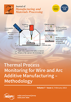
The Wire and Arc Additive Manufacturing (WAAM) process has a high potential for industrial applications in aviation. This study presents an approach to determine absolute values of the interlayer temperatures during the process using Ti-6Al-4V. The emissivity and transmittance are calibrated to enable a precise thermographic measurement. The methodology is validated by comparing the recorded data with signals from the thermocouples to align the absolute temperature values. Results show that with an interlayer temperature of 200 °C, heat accumulation occurs at the center of the layer due to faster cooling at the free ends. The methodology enables a non-tactile and reproducible measurement of the interlayer temperature during the WAAM process. View this paper
  • Issues are regarded as officially published after their release is announced to the table of contents alert mailing list.
  • You may sign up for e-mail alerts to receive table of contents of newly released issues.
  • PDF is the official format for papers published in both, html and pdf forms. To view the papers in pdf format, click on the "PDF Full-text" link, and use the free Adobe Reader to open them.
Order results
Result details
Select all
Export citation of selected articles as:
12 pages, 5689 KiB  
Article
Real-Time Cutting Temperature Measurement in Turning of AISI 1045 Steel through an Embedded Thermocouple—A Comparative Study with Infrared Thermography
by Bruno Guimarães, José Rosas, Cristina M. Fernandes, Daniel Figueiredo, Hernâni Lopes, Olga C. Paiva, Filipe S. Silva and Georgina Miranda
J. Manuf. Mater. Process. 2023, 7(1), 50; https://doi.org/10.3390/jmmp7010050 - 15 Feb 2023
Cited by 9 | Viewed by 3313
Abstract
During machining processes, a high temperature is generated in the cutting zone due to deformation of the material and friction of the chip along the surface of the tool. This high temperature has a detrimental effect on the cutting tool, and for this [...] Read more.
During machining processes, a high temperature is generated in the cutting zone due to deformation of the material and friction of the chip along the surface of the tool. This high temperature has a detrimental effect on the cutting tool, and for this reason, it is of the utmost importance to assess the cutting temperature in real time during these processes. Despite all the advances and investigation in this field, accurately measuring the cutting temperature remains a great challenge. In this sense, this work intends to contribute to solving this problem by experimentally evaluating the potential of the developed approach for embedding thermocouples into the rake face of cutting tools for measuring cutting temperature in real time during dry turning of AISI 1045 steel for different cutting parameters and comparing the obtained results with infrared thermography measurements at the exact same point. A well-defined, smooth micro-groove with good surface quality was produced by laser surface modification. Then a laser-welded K-type thermocouple was fixated in the micro-groove with a MgO ceramic adhesive, ensuring protection from wear and chips, which allowed the creation of WC-Co cutting inserts with the ability to measure cutting tool temperature with a maximum error of 0.96%. Results showed that, despite yielding the same trend, the tool temperature measured by the IR thermographic camera was always lower than the temperature measured by the K-type embedded thermocouple. The proposed embedded thermocouple method proved to be a reliable, precise, accurate, and cost-effective approach for real-time temperature measurement capable of providing useful information for cutting parameter optimization, thus allowing increased productivity and tool life. Full article
(This article belongs to the Special Issue Advances in Metal Cutting and Cutting Tools)
Show Figures

Figure 1

Figure 1
<p>Schematic representation of the K-type embedded thermocouple WC-Co insert.</p>
Full article ">Figure 2
<p>Micro-groove produced by laser surface modification: (<b>a</b>) top view SEM image; (<b>b</b>) tilt 45° SEM image; (<b>c</b>) 3D optical profilometry; and (<b>d</b>) surface topography profile.</p>
Full article ">Figure 3
<p>(<b>a</b>) SEM image of the laser-welded K-type thermocouple hot junction; (<b>b</b>) SEM image of the WC-Co cutting insert with the K-type embedded thermocouple.</p>
Full article ">Figure 4
<p>Calibration test of the K-type embedded thermocouple.</p>
Full article ">Figure 5
<p>Effect of cutting speed variation on the tool temperature over the machining time (a<sub>p</sub> = 1 mm).</p>
Full article ">Figure 6
<p>Effect of depth of cut variation on the tool temperature over the machining time (v<sub>c</sub> = 130 m/min).</p>
Full article ">Figure 7
<p>Example of IR thermographs obtained for experiment 1 over some machining times.</p>
Full article ">
22 pages, 11634 KiB  
Article
Study on Elucidation of the Roundness Improvement Mechanism of the Internal Magnetic Abrasive Finishing Process Using a Magnetic Machining Tool
by Jiangnan Liu and Yanhua Zou
J. Manuf. Mater. Process. 2023, 7(1), 49; https://doi.org/10.3390/jmmp7010049 - 13 Feb 2023
Cited by 4 | Viewed by 1936
Abstract
The magnetic abrasive finishing process using the magnetic machining tool was proposed to finish the internal surface of the thick tube (the thickness of the tube is 5~30 mm). It has been proved that this process can improve the roundness while improving the [...] Read more.
The magnetic abrasive finishing process using the magnetic machining tool was proposed to finish the internal surface of the thick tube (the thickness of the tube is 5~30 mm). It has been proved that this process can improve the roundness while improving the roughness. In this paper, we mainly study the machining mechanism of roundness improvement. Firstly, the influence of finishing characteristics on the roundness improvement was discussed, including the rotational speed of the magnetic machining tool and the rotational speed of the tube. It was concluded that the roundness improvement increases with the increase in the rotational speed through the analysis of finishing force and finishing times. Furthermore, the influence on roundness improvement of different distributions of magnetic particles were experimentally compared. After finishing, due to the magnetic force generated by the magnetic machining tool and the magnetic pole unit exerting pressure on the magnetic particles, a fixed magnetic brush is formed. The experimental results show that the circumferential length of the fixed magnetic brush is different due to the different distribution areas of magnetic particles. It was concluded that the roundness improvement increases with the circumferential length of the fixed magnetic brush increases by discussing the relationship between the circumferential length of the fixed magnetic brush and the wavelength of the roundness curve. When the circumferential length of the fixed magnetic brush is 76 mm, the roundness was improved from 379 μm to 236 μm after 60 min of finishing. Full article
(This article belongs to the Special Issue Advances in Metal Cutting and Cutting Tools)
Show Figures

Figure 1

Figure 1
<p>(<b>a</b>) Schematic of the internal magnetic abrasive finishing process using magnetic machining tool; (<b>b</b>) Force analysis model diagram of the magnetic machining tool.</p>
Full article ">Figure 1 Cont.
<p>(<b>a</b>) Schematic of the internal magnetic abrasive finishing process using magnetic machining tool; (<b>b</b>) Force analysis model diagram of the magnetic machining tool.</p>
Full article ">Figure 2
<p>Straight-line expansion of the internal surface of the tube along the circumference direction.</p>
Full article ">Figure 3
<p>External view of the experimental setup.</p>
Full article ">Figure 4
<p>Changes in material removal and surface roughness with finishing time.</p>
Full article ">Figure 5
<p>Roundness improvement with finishing time.</p>
Full article ">Figure 6
<p>Roundness profiles of the internal surface of the tube before and after finishing. (<b>a</b>) 32 rpm; (<b>b</b>) 122 rpm; (<b>c</b>) 212 rpm.</p>
Full article ">Figure 7
<p>Changes in material removal and surface roughness with finishing time.</p>
Full article ">Figure 8
<p>Roundness improvement with finishing time.</p>
Full article ">Figure 9
<p>Roundness profiles of the internal surface of the tube before and after finishing. (<b>a</b>) 35 rpm; (<b>b</b>) 115 rpm; (<b>c</b>) 195 rpm.</p>
Full article ">Figure 10
<p>Distribution of magnetic force lines of magnetic machining tool.</p>
Full article ">Figure 11
<p>Changes in material removal and surface roughness with finishing time.</p>
Full article ">Figure 12
<p>Roundness improvement with finishing time.</p>
Full article ">Figure 13
<p>Photographs of magnetic machining tool before and after finishing. (<b>a</b>) Before finishing; (<b>b</b>) After finishing.</p>
Full article ">Figure 14
<p>Roundness profiles of the internal surface of the tube before and after finishing. (<b>a</b>) Magnetic particles:12 g; (<b>b</b>) Magnetic particles:13 g; (<b>c</b>) Magnetic particles:14 g.</p>
Full article ">Figure 15
<p>Changes in material removal and surface roughness with finishing time.</p>
Full article ">Figure 16
<p>Roundness improvement with finishing time.</p>
Full article ">Figure 17
<p>Photographs of magnetic machining tool before and after finishing. (<b>a</b>) Before finishing; (<b>b</b>) After finishing.</p>
Full article ">Figure 17 Cont.
<p>Photographs of magnetic machining tool before and after finishing. (<b>a</b>) Before finishing; (<b>b</b>) After finishing.</p>
Full article ">Figure 18
<p>Roundness profiles of the internal surface of the tube before and after finishing. (<b>a</b>) Experiment A; (<b>b</b>) Experiment B; (<b>c</b>) Experiment C.</p>
Full article ">Figure 18 Cont.
<p>Roundness profiles of the internal surface of the tube before and after finishing. (<b>a</b>) Experiment A; (<b>b</b>) Experiment B; (<b>c</b>) Experiment C.</p>
Full article ">Figure 19
<p>Diagram of the relationship between the circumferential length of fixed magnetic brush and the wavelength of roundness curve. (<b>a</b>) L &lt; λ; (<b>b</b>) L ≥ λ.</p>
Full article ">
16 pages, 13839 KiB  
Article
Development of a Computationally Efficient Model of the Heating Phase in Thermoforming Process Based on the Experimental Radiation Pattern of Heaters
by Hadi Hosseinionari, Milad Ramezankhani, Rudolf Seethaler and Abbas S. Milani
J. Manuf. Mater. Process. 2023, 7(1), 48; https://doi.org/10.3390/jmmp7010048 - 10 Feb 2023
Cited by 3 | Viewed by 2039
Abstract
In this study, an accurate and computationally efficient model for the heating process of thin thermoplastic sheets during thermoforming is developed. This model opens the door to efficient training of model-free control approaches in thermoforming applications, which often require extensive training data that [...] Read more.
In this study, an accurate and computationally efficient model for the heating process of thin thermoplastic sheets during thermoforming is developed. This model opens the door to efficient training of model-free control approaches in thermoforming applications, which often require extensive training data that would be significantly costly and time-consuming to generate using physical setups. This model takes into account heat transfer via radiation between heaters and the sheet, heat transfer via conduction through the sheet, and heat transfer via convection between the sheet and the ambient. In this paper, rather than using an analytical relationship for the view factor, an experiment is designed to determine the exact radiation pattern of the heater on the sheet and the fraction of infrared emission absorbed by the sheet. Comparing the output temperature profile on the sheet from the designed model to IR images from a laboratory-scale heating system indicates that the mean square error is reduced by around four times when compared to traditional models with analytical view factors. Moreover, a comparison of the computation time with COMSOL software for a scenario with the same configuration of computation hardware reveals that the designed model is almost ten times faster. Full article
Show Figures

Figure 1

Figure 1
<p>The general reinforcement learning framework.</p>
Full article ">Figure 2
<p>Schematic of basic vacuum thermoforming. (<b>a</b>) Heating; (<b>b</b>) sealing or pre-stretch; (<b>c</b>) forming and cooling [<a href="#B4-jmmp-07-00048" class="html-bibr">4</a>].</p>
Full article ">Figure 3
<p>(<b>a</b>) Heat transfer between thermoplastic sheet, radiant heaters, and ambient; (<b>b</b>) elements for model.</p>
Full article ">Figure 4
<p>Heat transfer coefficient for free convection between the cold surrounding and hot plate [<a href="#B35-jmmp-07-00048" class="html-bibr">35</a>].</p>
Full article ">Figure 5
<p>Plate arrangements (parallel plates) [<a href="#B32-jmmp-07-00048" class="html-bibr">32</a>].</p>
Full article ">Figure 6
<p>(<b>a</b>) Laboratory-scale heating system setup; (<b>b</b>) number of heating elements.</p>
Full article ">Figure 7
<p>(<b>a</b>) Actual heater surface temperature variation over time for different power levels; (<b>b</b>) comparison the simulated and actual surface temperatures variation over time in different power consumption.</p>
Full article ">Figure 8
<p>Laboratory-scale setup: temperature distribution on the sheet using a trough ceramic heater with 500 W maximum power consumption at (<b>a</b>) t = 15 s; (<b>b</b>) t = 30 s; (<b>c</b>) t = 45 s; (<b>d</b>) t = 60 s.</p>
Full article ">Figure 9
<p>Reflected and absorbed radiation on opaque surface.</p>
Full article ">Figure 10
<p>Extracted experimental <math display="inline"><semantics> <mrow> <msub> <mi mathvariant="sans-serif">α</mi> <mi mathvariant="normal">a</mi> </msub> <mo>×</mo> <msub> <mi>F</mi> <mrow> <mi>h</mi> <mo>→</mo> <mi>m</mi> <mo>,</mo> <mi>n</mi> </mrow> </msub> </mrow> </semantics></math> for each element of the sheet (<b>a</b>) surface graph; (<b>b</b>) numerical values of <math display="inline"><semantics> <mrow> <msub> <mi mathvariant="sans-serif">α</mi> <mi mathvariant="normal">a</mi> </msub> <mo>×</mo> <msub> <mi>F</mi> <mrow> <mi>h</mi> <mo>→</mo> <mi>m</mi> <mo>,</mo> <mi>n</mi> </mrow> </msub> </mrow> </semantics></math> in contour graph.</p>
Full article ">Figure 11
<p>Heating elements number 4 and 8 with surface temperature of 603 K and 803 K, respectively.</p>
Full article ">Figure 12
<p>Temperature distribution on the sheet (<b>a</b>) laboratory-scale setup; (<b>b</b>) designed model based on experimental radiation pattern; (<b>c</b>) designed model based on analytical view factors.</p>
Full article ">Figure 13
<p>Actual and simulated temperature variations along three cut-line in the y direction of the thermoplastic sheet, (<b>a</b>) cut-line locations; (<b>b</b>) cut-line 1 temperatures; (<b>c</b>) cut-line 2 temperatures; (<b>d</b>) cut-line 3 temperatures.</p>
Full article ">Figure 14
<p>Actual and simulated temperature variations along three cut-line in the x direction of the thermoplastic sheet, (<b>a</b>) cut-line locations; (<b>b</b>) cut-line 1 temperatures; (<b>c</b>) cut-line 2 temperatures; (<b>d</b>) cut-line 3 temperatures.</p>
Full article ">Figure 15
<p>Temperature distribution on the sheet after 120 s (COMSOL Multiphysics V 5.6 software).</p>
Full article ">
2 pages, 185 KiB  
Editorial
Metal Additive Manufacturing and Its Post-Processing Techniques
by Hao Wang and Jerry Ying Hsi Fuh
J. Manuf. Mater. Process. 2023, 7(1), 47; https://doi.org/10.3390/jmmp7010047 - 10 Feb 2023
Cited by 2 | Viewed by 2778
Abstract
Metal additive manufacturing has made substantial progress in the advanced manufacturing sector with competitive advantages for the efficient production of high-quality products [...] Full article
(This article belongs to the Special Issue Metal Additive Manufacturing and Its Post Processing Techniques)
19 pages, 16807 KiB  
Article
Using 3D Density-Gradient Vectors in Evolutionary Topology Optimization to Find the Build Direction for Additive Manufacturing
by Dylan Bender and Ahmad Barari
J. Manuf. Mater. Process. 2023, 7(1), 46; https://doi.org/10.3390/jmmp7010046 - 9 Feb 2023
Cited by 3 | Viewed by 2047
Abstract
Given its layer-based nature, additive manufacturing is known as a family of highly capable processes for fabricating complex 3D geometries designed by means of evolutionary topology optimization. However, the required support structures for the overhanging features of these complex geometries can be concerningly [...] Read more.
Given its layer-based nature, additive manufacturing is known as a family of highly capable processes for fabricating complex 3D geometries designed by means of evolutionary topology optimization. However, the required support structures for the overhanging features of these complex geometries can be concerningly wasteful. This article presents an approach for studying the manufacturability of the topology-optimized complex 3D parts required for additive manufacturing and finding the optimum corresponding build direction for the fabrication process. The developed methodology uses the density gradient of the design matrix created during the evolutionary topology optimization of the 3D domains to determine the optimal build orientation for additive manufacturing with the objective of minimizing the need for support structures. Highly satisfactory results are obtained by implementing the developed methodology in analytical and experimental studies, which demonstrate potential additive manufacturing mass savings of 170% of the structure’s weight. The developed methodology can be readily used in a variety of evolutionary topology optimization algorithms to design complex 3D geometries for additive manufacturing technologies with a minimized level of waste due to reducing the need for support structures. Full article
Show Figures

Figure 1

Figure 1
<p>The process of structural design by means of topology optimization: (1) define the design problem; (2) discretize the design domain; and (3) optimize the structure’s topology to achieve an efficient design.</p>
Full article ">Figure 2
<p>Global node IDs in a prismatic structure composed of 8 elements and 30 nodes.</p>
Full article ">Figure 3
<p>The detail shows part of the density field with the approximated gradients of the density field. The gradient vectors point in the direction of increasing density [<a href="#B22-jmmp-07-00046" class="html-bibr">22</a>].</p>
Full article ">Figure 4
<p>Two examples of a pair of masks used to approximate the Cartesian components of an image’s intensity gradient.</p>
Full article ">Figure 5
<p>A visualization of the elemental density gradient vector at an element.</p>
Full article ">Figure 6
<p>Density configurations that are misinterpreted by the Sobel/Prewitt kernels.. Both subfigures (<b>A</b>) and (<b>B</b>) show that the density gradient approximation via matrix convolution is 45° rather than the naturally perceived overhanging angle of 90°.</p>
Full article ">Figure 7
<p>Print orientations that maximize (<b>left</b>) and minimize (<b>right</b>) the required volume of supporting structure [<a href="#B40-jmmp-07-00046" class="html-bibr">40</a>].</p>
Full article ">Figure 8
<p>Masks that are used to approximate the gradient across the x-plane. These masks are akin to the 2D Prewitt masks for image processing.</p>
Full article ">Figure 9
<p>Masks that are used to approximate the gradient across each of the cartesian planes. These masks are akin to the Sobel masks for image processing.</p>
Full article ">Figure 10
<p>A sample overhanging surface angle analysis of a cantilever: (<b>left</b>) facets of the finite elements are colored and (<b>right</b>) a smoothed isosurface.</p>
Full article ">Figure 11
<p>Examples of the fabricated samples for the experimental topologically optimized cantilever beam: (<b>a</b>) orientation with maximum required support volume; and (<b>b</b>) orientation with minimum required support volume.</p>
Full article ">
24 pages, 2140 KiB  
Review
A Review on Wire-Fed Directed Energy Deposition Based Metal Additive Manufacturing
by Tuğrul Özel, Hamed Shokri and Raphaël Loizeau
J. Manuf. Mater. Process. 2023, 7(1), 45; https://doi.org/10.3390/jmmp7010045 - 8 Feb 2023
Cited by 16 | Viewed by 7296
Abstract
Metal additive manufacturing has reached a level where products and components can be directly fabricated for applications requiring small batches and customized designs, from tinny body implants to long pedestrian bridges over rivers. Wire-fed directed energy deposition based additive manufacturing enables fabricating large [...] Read more.
Metal additive manufacturing has reached a level where products and components can be directly fabricated for applications requiring small batches and customized designs, from tinny body implants to long pedestrian bridges over rivers. Wire-fed directed energy deposition based additive manufacturing enables fabricating large parts in a cost-effective way. However, achieving reliable mechanical properties, desired structural integrity, and homogeneity in microstructure and grain size is challenging due to layerwise-built characteristics. Manufacturing processes, alloy composition, process variables, and post-processing of the fabricated part strongly affect the resultant microstructure and, as a consequence, component serviceability. This paper reviews the advances in wire-fed directed energy deposition, specifically wire arc metal additive processes, and the recent efforts in grain tailoring during the process for the desired size and shape. The paper also addresses modeling methods that can improve the qualification of fabricated parts by modifying the microstructure and avoid repetitive trials and material waste. Full article
(This article belongs to the Special Issue Editorial Board Members’ Collection Series: Additive Manufacturing)
Show Figures

Figure 1

Figure 1
<p>Categories of directed energy deposition in terms of energy source and feedstock.</p>
Full article ">Figure 2
<p>(<b>a</b>) Laser, powder-fed DED (LP-DED) system [<a href="#B24-jmmp-07-00045" class="html-bibr">24</a>]; (<b>b</b>) laser, wire-fed DED (LW-DED) system [<a href="#B25-jmmp-07-00045" class="html-bibr">25</a>], (<b>c</b>) electron beam, wire-fed DED (EB-DED) system [<a href="#B26-jmmp-07-00045" class="html-bibr">26</a>]; (<b>d</b>) electric arc, wire-fed DED (WA-DED) system [<a href="#B27-jmmp-07-00045" class="html-bibr">27</a>]; (<b>e</b>) WA-DED model of a 3.94-foot (1.2 m) Ti6Al4V wing spar [<a href="#B10-jmmp-07-00045" class="html-bibr">10</a>]; and (<b>f</b>) PW-DED aircraft structural component from Ti6Al4V using Norsk Titanium’s rapid plasma Deposition process [<a href="#B10-jmmp-07-00045" class="html-bibr">10</a>]. Images in (<b>a</b>), (<b>b</b>), (<b>c</b>), (<b>d</b>) are reproduced with permission from authors in [<a href="#B24-jmmp-07-00045" class="html-bibr">24</a>,<a href="#B25-jmmp-07-00045" class="html-bibr">25</a>,<a href="#B26-jmmp-07-00045" class="html-bibr">26</a>,<a href="#B27-jmmp-07-00045" class="html-bibr">27</a>] respectively. Images in (<b>b</b>), (<b>c</b>), (<b>e</b>) and (<b>f</b>) are reproduced with permissions from Procada, Sciaky, Welding and Additive Manufacturing Centre, Cranfield University, and Norsk Titanium respectively.</p>
Full article ">Figure 3
<p>Small melt pools, high cooling rates (T), growth velocities (<span class="html-italic">v</span>), and thermal gradients (G) during the majority of AM processes favor the formation of columnar dendrites. The figure is adopted with permission from authors in [<a href="#B46-jmmp-07-00045" class="html-bibr">46</a>].</p>
Full article ">Figure 4
<p>The correlation between materials and defects in WAAM processes.</p>
Full article ">Figure 5
<p>Mechanical properties (in build direction, ultimate tensile strength (UTS), and yield strength (YS)) of Ti-6Al-4V-fabricated from various WAAM processes (AF: as fabricated, HT: heat treated, GTAW: gas tungsten arc welding, PAW: plasma arc welding).</p>
Full article ">
23 pages, 8556 KiB  
Article
Influence of Ambient Temperature and Crystalline Structure on Fracture Toughness and Production of Thermoplastic by Enclosure FDM 3D Printer
by Supaphorn Thumsorn, Wattanachai Prasong, Akira Ishigami, Takashi Kurose, Yutaka Kobayashi and Hiroshi Ito
J. Manuf. Mater. Process. 2023, 7(1), 44; https://doi.org/10.3390/jmmp7010044 - 8 Feb 2023
Cited by 7 | Viewed by 3206
Abstract
Fused deposition modeling (FDM) 3D printing has printed thermoplastic materials layer-by-layer to form three dimensional products whereby interlayer adhesion must be well controlled to obtain high mechanical performance and product integrity. This research studied the effects of ambient temperatures and crystalline structure on [...] Read more.
Fused deposition modeling (FDM) 3D printing has printed thermoplastic materials layer-by-layer to form three dimensional products whereby interlayer adhesion must be well controlled to obtain high mechanical performance and product integrity. This research studied the effects of ambient temperatures and crystalline structure on the interlayer adhesion and properties of thermoplastic FDM 3D printing. Five kinds of poly(lactic acid) (PLA) filaments, both commercially available and the laboratory-made, were printed using the enclosure FDM 3D printer. The ambient temperatures were set by the temperature-controlled chamber from room temperature to 75 °C with and without a cooling fan. The interlayer adhesion was characterized by the degree of entanglement density, morphology, and fracture toughness. In addition, PLA filament with high crystallinity has induced heat resistance, which could prevent filament clogging and successfully print at higher chamber temperatures. The ambient temperature increased with increased chamber temperature and significantly increased when printed without a cooling fan, resulting in improved interlayer bonding. The crystalline structure and dynamic mechanical properties of the 3D printed products were promoted when the chamber temperature was increased without a cooling fan, especially in PLA composites and PLA containing a high content of L-isomer. However, although the additives in the PLA composite improved crystallinity and the degree of entanglement density in the 3D-printed products, they induced an anisotropic characteristic that resulted in the declination of the interlayer bonding in the transverse orientation products. The increasing of chamber temperatures over 40 °C improved the interlayer bonding in pristine PLA products, which was informed by the increased fracture toughness. Further, it can be noted that the amorphous nature of PLA promotes molecular entanglement, especially when printed at higher chamber temperatures with and without a cooling fan. Full article
Show Figures

Figure 1

Figure 1
<p>FDM 3D printing dimensions (unit in mm) and direction; (<b>a</b>) Dumbbell specimen and (<b>b</b>) Compact tension specimen.</p>
Full article ">Figure 2
<p>Drawing of FUNMAT HT FDM 3D printer with temperature-controlled chamber.</p>
Full article ">Figure 3
<p>WAXD patterns of PLA filaments and 3D printed dumbbell specimens at chamber temperatures of 40 °C and 45 °C; (<b>a1</b>–<b>e1</b>) PLA filaments, (<b>a2</b>–<b>e2</b>) with cooling fan and (<b>a3</b>–<b>e3</b>) without cooling fan.</p>
Full article ">Figure 4
<p>WAXD intensities (<b>a</b>) PLA filaments and (<b>b</b>) 3D Printed dumbbell specimens at chamber temperatures of 40 °C and 45 °C with and without cooling fan.</p>
Full article ">Figure 5
<p>DSC thermograms of PLA filaments; (<b>a</b>) Total heat flow, (<b>b</b>) Nonreversible heat flow and (<b>c</b>) Reversible heat flow.</p>
Full article ">Figure 6
<p>DSC thermograms of 3D printed dumbbell specimens at chamber temperature 40 °C and 45 °C printed with cooling fan; (<b>a</b>) Total heat flow and (<b>b</b>) Reversible heat flow.</p>
Full article ">Figure 7
<p>DSC thermograms of 3D printed dumbbell specimens at chamber temperature 40 °C and 45 °C printed without cooling fan; (<b>a</b>) Total heat flow and (<b>b</b>) Reversible heat flow.</p>
Full article ">Figure 8
<p>Dynamic mechanical properties of 3D printed dumbbell specimens at chamber temperatures of 40 °C and 45 °C with and without cooling fan; (<b>a</b>) storage modulus and (<b>b</b>) Tan δ.</p>
Full article ">Figure 9
<p>Thermal profile images of 3D printed compact tension specimens at chamber temperatures of 40 °C, 45 °C and 75 °C; (<b>a1</b>–<b>e1</b>) printed with cooling fan and (<b>a2</b>–<b>e2</b>) printed without cooling fan.</p>
Full article ">Figure 10
<p>Load-displacement curves of 3D printed compact tension test at virous chamber temperatures printed with and without cooling fan; (<b>a</b>) PLA-AH, (<b>b</b>) PLA-N and (<b>c</b>) PLA-P and PLA-CF.</p>
Full article ">Figure 11
<p>Fracture toughness (K<sub>IC</sub>) of 3D printed compact tension test at virous chamber temperatures; (<b>a</b>) with cooling fan and (<b>b</b>) without cooling fan.</p>
Full article ">Figure 12
<p>SEM images from side view of 3D printed compact tension fractured surfaces at various chamber temperatures (white arrow indicates notched area); (<b>a1</b>–<b>d1</b>) PLA-AH with cooling fan, (<b>a2</b>–<b>d2</b>) PLA-N, PLA-P and PLA-CF with cooling fan, (<b>a3</b>–<b>d3</b>) PLA-AH without cooling fan and (<b>a4</b>–<b>d4</b>) PLA-N, PLA-P and PLA-CF without cooling fan.</p>
Full article ">Figure 13
<p>SEM images from top view and magnified images of 3D printed compact tension fractured surfaces at various chamber temperatures (white arrow indicates an observation area that magnified by red arrow); (<b>a1</b>–<b>d1</b>) PLA-AH and PL-N with cooling fan, (<b>a2</b>–<b>d2</b>) PLA-AH and PLA-N without cooling fan, (<b>a3</b>–<b>b3</b>) PLA-P and PLA-CF with cooling fan and (<b>c3</b>–<b>d3</b>) PLA-P and PLA-CF without cooling fan.</p>
Full article ">
16 pages, 2037 KiB  
Article
Building Orientation and Post Processing of Ti6Al4V Produced by Laser Powder Bed Fusion Process
by Rosaria Rovetta, Paola Ginestra, Rosalba Monica Ferraro, Keren Zohar-Hauber, Silvia Giliani and Elisabetta Ceretti
J. Manuf. Mater. Process. 2023, 7(1), 43; https://doi.org/10.3390/jmmp7010043 - 7 Feb 2023
Cited by 8 | Viewed by 2361
Abstract
Laser powder bed fusion, particularly the selective laser melting (SLM), is an additive manufacturing (AM) technology used to produce near-net-shaped engineering components for biomedical applications, especially in orthopaedics. Ti6Al4V is commonly used for producing orthopaedic implants using SLM because it has excellent mechanical [...] Read more.
Laser powder bed fusion, particularly the selective laser melting (SLM), is an additive manufacturing (AM) technology used to produce near-net-shaped engineering components for biomedical applications, especially in orthopaedics. Ti6Al4V is commonly used for producing orthopaedic implants using SLM because it has excellent mechanical qualities, a high level of biocompatibility, and corrosion resistance. However, the main problems associated with this process are the result of its surface properties: it has to be able to promote cell attachment but, at the same time, avoid bacteria colonization. Surface modification is used as a post-processing technique to provide items the unique qualities that can improve their functionality and performance in particular working conditions. The goal of this work was to produce and analyse Ti6Al4V samples fabricated by SLM with different building directions in relation to the building plate (0° and 45°) and post-processed by anodization and passivation. The results demonstrate how the production and post processes had an impact on osteoblast attachment, mineralization, and osseointegration over an extended period of time. Though the anodization treatment result was cytotoxic, the biocompatibility of as-built specimens and specimens after passivation treatment was confirmed. In addition, it was discovered that effective post-processing increases the mineralization of these types of 3D-printed surfaces. Full article
Show Figures

Figure 1

Figure 1
<p>Micrographs illustrating the surface topography of the Ti6Al4V samples manufactured by SLM at 0° and 45°: as-built (<b>a</b>), with post-processing treatments anodization (<b>b</b>) and etching (<b>c</b>).</p>
Full article ">Figure 2
<p>CA measurements for the samples: (<b>a</b>) 0° building angle individual samples; (<b>b</b>) 45° building angle individual samples; (<b>c</b>) images of the water droplets on the top surfaces at different building angles and treatments.</p>
Full article ">Figure 3
<p>Sa measurements for the samples: (<b>a</b>) 0° building angle individual samples; (<b>b</b>) 0° building angle individual samples.</p>
Full article ">Figure 4
<p>Micrographs illustrating the surface profile of the cross-sections of the samples built at different building angles and with different treatments.</p>
Full article ">Figure 5
<p>ATP (μm) concentrations of MC3T3-E1 cells cultured on titanium as-built, anodized and etched 0° and 45° SLM scaffolds and on a plastic dish after 24 h, 48 h, and 96 h. Unpaired <span class="html-italic">t</span>-test was applied to discriminate differences between MC3T3-E1 cultured on a plastic dish and on each scaffold considering a statistically significant value of <span class="html-italic">p</span> &lt; 0.05 (** <span class="html-italic">p</span> &lt; 0.01, *** <span class="html-italic">p</span> &lt; 0.001, **** <span class="html-italic">p</span> &lt; 0.0001).</p>
Full article ">Figure 6
<p>ATP (μm) concentrations of MC3T3-E1 cells cultured in conditioned and in control medium at different time points (24 h, 48 h, and 96 h). Unpaired <span class="html-italic">t</span>-test was applied to discriminate differences between MC3T3-E1 cultured on a plastic dish and on each scaffold considering a statistically significant value of <span class="html-italic">p</span> &lt; 0.05 (**** <span class="html-italic">p</span> &lt; 0.0001).</p>
Full article ">Figure 7
<p>Gene expression evaluation of MC3T3-E1 cells cultured in mineralization medium after 30 days on titanium as-built and etched (0° and 45°) SLM scaffolds and on a plastic well plate. Unpaired <span class="html-italic">t</span>-test was applied to discriminate differences between plastic dish and each scaffold considering a statistically significant value of <span class="html-italic">p</span> &lt; 0.05 (* <span class="html-italic">p</span> &lt; 0.05, ** <span class="html-italic">p</span> &lt; 0.01, *** <span class="html-italic">p</span> &lt; 0.001,). Unpaired <span class="html-italic">t</span>-test was used also to compare as-built substrates and relative etched scaffolds (“ns” indicates not significant, <span class="html-italic">p</span> &gt; 0.05).</p>
Full article ">
14 pages, 8134 KiB  
Article
Investigation of the Pull-Out Behaviour of Metal Threaded Inserts in Thermoplastic Fused-Layer Modelling (FLM) Components
by Tobias Kastner, Juliane Troschitz, Christian Vogel, Thomas Behnisch, Maik Gude and Niels Modler
J. Manuf. Mater. Process. 2023, 7(1), 42; https://doi.org/10.3390/jmmp7010042 - 7 Feb 2023
Cited by 2 | Viewed by 2215
Abstract
To provide detachable, secure and long-term stable joints in fused-layer modelling (FLM) components or assemblies, metal threaded inserts are widely used as extrinsic interfaces. However, the load-bearing capacity of such inserts is influenced by the inhomogeneous, anisotropic material structure of the FLM components. [...] Read more.
To provide detachable, secure and long-term stable joints in fused-layer modelling (FLM) components or assemblies, metal threaded inserts are widely used as extrinsic interfaces. However, the load-bearing capacity of such inserts is influenced by the inhomogeneous, anisotropic material structure of the FLM components. This work evaluates the influence of the joining zone design and the printing process parameters on the achievable joint properties. Therefore, we printed thermoplastic FLM test specimens with varying parameters for infill density, wall thickness, layer height and nozzle temperature. Subsequently, metal threaded inserts were warm-embedded into the test specimens and investigated in quasi-static pull-out tests. The results show that the infill density in the joining zone has the largest impact on the joint strength and should be 70% or higher. Furthermore, an analysis of different wall thicknesses around the pre hole shows that a minimum value of 2.4 mm is required for the selected insert geometry to achieve a high pull-out force. Increasing the wall thickness beyond this value does not significantly affect the joint strength. The results provide an improved base for detailed understanding and interface design in FLM components for the integration of metal threaded inserts as well as for further investigations regarding different printing materials and load types. Full article
Show Figures

Figure 1

Figure 1
<p>Demonstrating the use of metal threaded inserts in FLM components for retrofitting sensors for autonomous driving within the ABSOLUT project: (<b>a</b>) automated electric VW e-Crafter with three independent sensor systems and upgraded add-on X-by-Wire-System, (<b>b</b>) detailed view of a 360° lidar sensor mounted with a FLM connector and (<b>c</b>) FLM connector with integrated metal threaded inserts.</p>
Full article ">Figure 2
<p>Schematic illustration of the FLM test specimen.</p>
Full article ">Figure 3
<p>Schematic illustration of the orientation of the layer structure in the FLM test specimen: (<b>a</b>) layer orientation in the <span class="html-italic">x</span>–<span class="html-italic">y</span> plane and (<b>b</b>) layer orientation in the <span class="html-italic">x</span>–<span class="html-italic">z</span> plane.</p>
Full article ">Figure 4
<p>(<b>a</b>) Set up of the warm embedding of inserts into FLM test specimens and (<b>b</b>) cross section of FLM test specimen with embedded insert.</p>
Full article ">Figure 5
<p>Schematic illustration of the pull-out test setup (all dimensions in mm).</p>
Full article ">Figure 6
<p>Exemplary characteristic force-displacement graphs of the pull-out tests for variations of the infill density.</p>
Full article ">Figure 7
<p>Maximum pull-out forces for variations of the infill density (six specimens each).</p>
Full article ">Figure 8
<p>Exemplary test specimens of the test series with varying infill density: top view (<b>a</b>–<b>c</b>) and sectional view (<b>d</b>–<b>f</b>).</p>
Full article ">Figure 9
<p>Characteristic force-displacement graphs of the pull-out tests for variations of the wall thickness.</p>
Full article ">Figure 10
<p>Maximum pull-out forces for variations of the wall thickness (six specimens each).</p>
Full article ">Figure 11
<p>Exemplary test specimens of the test series with varying wall thickness and corresponding sectional views: top view (<b>a</b>–<b>c</b>) and sectional view (<b>d</b>–<b>f</b>).</p>
Full article ">Figure 12
<p>Characteristic force-displacement graphs of the pull-out tests for variations of the layer height.</p>
Full article ">Figure 13
<p>Maximum pull-out forces for variations of the layer height (six specimens each).</p>
Full article ">Figure 14
<p>Exemplary test specimens of the test series with varying layer heights: top view (<b>a</b>–<b>c</b>) and sectional view (<b>d</b>–<b>f</b>).</p>
Full article ">Figure 15
<p>Characteristic force-displacement graphs of the pull-out tests for variations of the temperature.</p>
Full article ">Figure 16
<p>Maximum pull-out forces for variations of the nozzle temperature (six specimens each).</p>
Full article ">Figure 17
<p>Exemplary test specimens of the test series with varying nozzle temperature: top view (<b>a</b>,<b>b</b>) and sectional view (<b>c</b>,<b>d</b>).</p>
Full article ">
29 pages, 7556 KiB  
Article
Development and Practical Implementation of Digital Observer for Elastic Torque of Rolling Mill Electromechanical System
by Vadim R. Gasiyarov, Andrey A. Radionov, Boris M. Loginov, Alexander S. Karandaev, Olga A. Gasiyarova and Vadim R. Khramshin
J. Manuf. Mater. Process. 2023, 7(1), 41; https://doi.org/10.3390/jmmp7010041 - 4 Feb 2023
Cited by 11 | Viewed by 2017
Abstract
The strategic initiative aimed at building “digital metallurgy” implies the introduction of diagnostic monitoring systems to trace the technical condition of critical production units. This problem is relevant for rolling mills, which provide the output and determine the quality of products of metallurgical [...] Read more.
The strategic initiative aimed at building “digital metallurgy” implies the introduction of diagnostic monitoring systems to trace the technical condition of critical production units. This problem is relevant for rolling mills, which provide the output and determine the quality of products of metallurgical companies. Making up monitoring systems requires the development of digital shadows and coordinate observers, the direct measurement of which is either impossible or associated with numerous difficulties. These coordinates include the spindle torque applied by the spring-transmitting torque from the motor to the rolling stand rolls. The development and research are conducted by the example of the electromechanical systems of the horizontal stand at the plate mill 5000. The stand electric drive characteristics are given, and the emergency modes that cause mechanical equipment breakdowns are analyzed that. The relevance of analyzing transient torque processes in emergency modes has been accentuated. The paper points to the shortcomings of the system for elastic torque direct measurement, including low durability due to the harsh operating conditions of precision sensors. It also highlights the need to install the measuring equipment after each spindle. The disadvantage of the previously developed observer is the function of calculating the electric drive speed derivative. This causes a decrease in noise immunity and signal recovery accuracy. The contribution of this paper is building a digital elastic torque observer that has advantages over conventional technical solutions, based on the theoretical and experimental studies. The technique for virtual observer adjustment was developed and tested in the Matlab-Simulink software package. For the first time, a comprehensive analysis was conducted for spindle elastic torques in emergency modes that caused equipment damage. An algorithm was developed for an emergency shutdown of a stand electric drive in the worst-case mode of strip retraction between work and backup rolls, due to the overlap of the strip on the roll. Further, the algorithm was tested experimentally. The criteria for diagnosing pre-emergencies was then justified. An adaptive motor-braking rate controller was developed. The developed observer and emergency braking system are in operation at the mill 5000. Long experimental research proved the efficiency of dynamic load monitoring and the reduction in the number of equipment breakdowns. Full article
Show Figures

Figure 1

Figure 1
<p>Individual Drive of the Rolling stand (<b>a</b>) and Kinematic Diagram of the Rolls (<b>b</b>): 1 is the frame; 2 and 3 are electromechanical and hydraulic screw-downs, respectively; 4 and 5 are the backup and work rolls, respectively; 6 is retractable spindles; 7 is the counterbalance; 8 is the motors.</p>
Full article ">Figure 2
<p>Installing the Torque Sensor on the Mill 5000 Horizontal Stand Spindle (<b>a</b>) and the layout of the strain gauges (<b>b</b>): 1—sensor; 2—telemetry ring; 3—telescopic shaft.</p>
Full article ">Figure 3
<p>Diagram Describing the Principle of Torque Recovery in a Conventional Observer.</p>
Full article ">Figure 4
<p>The Accident Consequences: Sheet Overlap on the Bottom Roll (<b>a</b>) and the Spindle Head Breakage (<b>b</b>).</p>
Full article ">Figure 5
<p>Kinematic diagram of the transmission (<b>a</b>) and block diagram of the two-mass electromechanical system (<b>b</b>): 1 is the is the speed controller; 2 is speed closed loop; 3, 8 is the transfer functions of the 1st and the 2nd inertia elements of the two-mass system (motor and roll); 4 is the integrator; 5 is the block simulating the angular gap; 6 is the mechanical transmission elastic coefficient; 7 is the elastic vibrations damping block; 9 is the first mass speed feedback coefficient.</p>
Full article ">Figure 6
<p>Model Diagram Describing the Observer Development (<b>a</b>) and the Structure of the Torque Observer Developed (<b>b</b>): block designations correspond to those shown in <a href="#jmmp-07-00041-f005" class="html-fig">Figure 5</a>.</p>
Full article ">Figure 7
<p>Spindle Torque Observer Connection Diagram (<b>a</b>), The Observer Model in Matlab-Simulink (<b>b</b>), and The PI Controller’s Discrete Model (<b>c</b>).</p>
Full article ">Figure 8
<p>Elastic torque oscillogram at capture (<b>a</b>) and LAFC, used for setting (<b>b</b>).</p>
Full article ">Figure 9
<p>Oscillograms Recorded at the Drive Successive Acceleration and Deceleration (<b>a</b>) and in the Metal Bite Mode (<b>b</b>): <span class="html-italic">n</span><sub>motor</sub>—the motor rotational velocity, % of the rated value; <span class="html-italic">M</span><sub>motor</sub><span class="html-italic">—</span>the motor torque; <span class="html-italic">M</span><sub>shaft (act)</sub>—the spindle torque read by the sensor; <span class="html-italic">M</span><sub>shaft (calc)</sub>—the torque shown by the observer; <span class="html-italic">M</span><sub>shaft (dyn)</sub>—the dynamic torque shown by the observer.</p>
Full article ">Figure 10
<p>Oscillograms of the rotation speeds and torques at the breakdown of the stand lower roll obtained at the mill 5000 by means of the processing of experimental data arrays recorded by the PDA system: window 1—set and actual speeds of the upper and lower roll motors (<span class="html-italic">n</span><sub>BMD</sub> and <span class="html-italic">n</span><sub>TMD</sub>, respectively); window 2—TMD motor torque, kN∙m; window 3—BMD motor torque; window 4—rolling force.</p>
Full article ">Figure 11
<p>Motor and torque oscillograms at roll breakage similar to those given in <a href="#jmmp-07-00041-f010" class="html-fig">Figure 10</a>, recovered by the observer: window 1—actual TMD and BMD speeds (<span class="html-italic">n</span><sub>BMD</sub> and <span class="html-italic">n</span><sub>TMD</sub>, respectively); window 2—motor torque <span class="html-italic">M</span><sub>TMD</sub>, spindle torque <span class="html-italic">M</span><sub>SU</sub> of the upper roll and static load torque <span class="html-italic">M</span><sub>ST</sub>; window 3—the same dependencies for BMD.</p>
Full article ">Figure 12
<p>Velocity (window 1) and Torque (window 2) Oscillograms at Strip Overlap: <span class="html-italic">V</span><sub>0_TMD</sub>, <span class="html-italic">V</span><sub>0_BMD</sub>—TMD and BMD motor linear speed setting; <span class="html-italic">V</span><sub>TMD</sub>, <span class="html-italic">V</span><sub>BMD</sub>—TMD and BMD motor linear speed; <span class="html-italic">M</span><sub>TMD</sub>, <span class="html-italic">M</span><sub>BMD</sub>—TMD and BMD motor torque; <span class="html-italic">M</span><sub>ST</sub>, <span class="html-italic">M</span><sub>SB—</sub>top and bottom roll spindle torque; <span class="html-italic">M</span><sub>STmax</sub>, <span class="html-italic">M</span><sub>SBmax</sub>—maximum top and bottom roll spindle torque; <span class="html-italic">M</span><sub>motor_max</sub>—motor torque limit (240% of rated value). Lines 2 and 1—the limit and the intensive braking setting, respectively.</p>
Full article ">Figure 13
<p>Oscillograms of the studied emergency mode similar to those given in <a href="#jmmp-07-00041-f012" class="html-fig">Figure 12</a> (<b>a</b>) and the operation mode at the metal bite with the rolls (<b>b</b>): window 1—setting linear speeds <span class="html-italic">V</span><sub>0_TMD</sub>, <span class="html-italic">V</span><sub>0_BMD</sub> and motor linear rotation speeds <span class="html-italic">V</span><sub>TMD</sub>, <span class="html-italic">V</span><sub>BMD</sub>; window 2—motor and spindle torques; window 3—spindle derivative torques; window 4—the rolled part length, m; the torque designation corresponds to those in <a href="#jmmp-07-00041-f011" class="html-fig">Figure 11</a>.</p>
Full article ">Figure 13 Cont.
<p>Oscillograms of the studied emergency mode similar to those given in <a href="#jmmp-07-00041-f012" class="html-fig">Figure 12</a> (<b>a</b>) and the operation mode at the metal bite with the rolls (<b>b</b>): window 1—setting linear speeds <span class="html-italic">V</span><sub>0_TMD</sub>, <span class="html-italic">V</span><sub>0_BMD</sub> and motor linear rotation speeds <span class="html-italic">V</span><sub>TMD</sub>, <span class="html-italic">V</span><sub>BMD</sub>; window 2—motor and spindle torques; window 3—spindle derivative torques; window 4—the rolled part length, m; the torque designation corresponds to those in <a href="#jmmp-07-00041-f011" class="html-fig">Figure 11</a>.</p>
Full article ">Figure 14
<p>The Structure of the Control System Ensuring Emergency Braking at the Strip Overlap on the Roll.</p>
Full article ">Figure 15
<p>Linear speed setting diagram (a) in the system of emergency braking (<b>a</b>) and the adaptive RC output signals (<b>b</b>): <span class="html-italic">V</span><sub>1</sub>, <span class="html-italic">V</span><sub>2</sub>, <span class="html-italic">V</span><sub>3</sub> of setting speeds for the mechanisms located after the stand, for the stand motors, and for the mechanisms located before the stand, respectively; <span class="html-italic">U</span><sub>3</sub>—RC<sub>3</sub> output signal.</p>
Full article ">Figure 16
<p>Oscillograms of the Bite with Subsequent Emergency Shutdown at the action of the system developed for the first emergency case on Different Time Scales (<b>a</b>,<b>b</b>): window 1—set and actual TMD and BMD linear velocities; window 2—motor and spindle torques shown by observers; window 3—rolling force. The oscillogram legend corresponds to the legend agreed in previous Figures.</p>
Full article ">Figure 17
<p>Oscillograms at the Emergency Mill Shutdown Using the System for the Second Emergency Case.</p>
Full article ">
18 pages, 6843 KiB  
Article
Investigation of Pressure Fields Generated by Two Simultaneous Discharges in Liquid Initiated by Wires
by Mykhaylo Knyazyev, Maik Holzmüller and Werner Homberg
J. Manuf. Mater. Process. 2023, 7(1), 40; https://doi.org/10.3390/jmmp7010040 - 2 Feb 2023
Cited by 2 | Viewed by 1582
Abstract
The pressure fields generated by two simultaneous discharges have not been investigated on any notable scale for the electrohydraulic impulse forming method. In this study, the synchronicity of two discharges is ensured by the sequential connection of two wires mounted in two spark [...] Read more.
The pressure fields generated by two simultaneous discharges have not been investigated on any notable scale for the electrohydraulic impulse forming method. In this study, the synchronicity of two discharges is ensured by the sequential connection of two wires mounted in two spark gaps in a common volume of liquid. The objective is to experimentally confirm the equilibrium of the energies evolved in two spark gaps by means of pressure measurements. In addition, multipoint membrane pressure gauges demonstrated the feasibility of easily recording detailed pressure maps. Based on the membrane deformation mechanism and material strengthening under static and impulse conditions, the processing procedure is further developed so as to achieve better accuracy in the determination of pressure field parameters. The practical equality of the pressure fields on the left and right halves of the flat-loaded area confirms the equality of energies evolved in the two spark gaps. The direct shock waves create zones with the most intensive loading. These results provide a basis for the development of new electrohydraulic technologies involving the application of two simultaneous discharges with equal energy and pressure parameters. Full article
Show Figures

Figure 1

Figure 1
<p>Schematic diagram of the experimental setup: 1—pulse generator; 2—discharge chamber filled with water; 3—isolated electrode; 4—wire; 5—nut; 6—metallic membrane; 7—multipoint pressure-gauge body; 8—hole of 6 mm diameter; 9—stud.</p>
Full article ">Figure 2
<p>General view of the experimental tooling (<b>a</b>), discharge chamber with electrodes and wire fixation (<b>b</b>), multipoint pressure gauge body and metallic membrane after impulse loading (<b>c</b>), dial indicator with adaptor for 6 mm dimples (<b>d</b>); Numbering is the same as in <a href="#jmmp-07-00040-f001" class="html-fig">Figure 1</a>.</p>
Full article ">Figure 3
<p>Schematic diagram of membrane deformation into the hole of the pressure gauge.</p>
Full article ">Figure 4
<p>Approximation of test engineering stress-strain curves: σ<sub>test1</sub>(ε)—segment of representative curve based on single test data; σ<sub>app1</sub>(ε)—approximation function for single representative test; R<sup>2</sup>—coefficient of determination; σ<sub>s</sub>(ε)—curve of general approximation function based on mean values of 10 tests; R<sub>p0.2</sub>—proof strength at plastic extension 0.2%; R<sub>m</sub>—tensile strength at plastic A<sub>g</sub> and total A<sub>gt</sub> extensions; σ<sub>p</sub>—stress limit of proportionality at elastic strain ε<sub>e0</sub> = 0.2%; ε<sub>p</sub> and ε<sub>e</sub>—elastic and plastic components of total strain (deformation) for flow stress value σ<sub>s</sub>.</p>
Full article ">Figure 5
<p>Three-dimensional representation of the pressure field generated by the simultaneous explosion of the two wires plotted from the mean test values.</p>
Full article ">Figure 6
<p>Contour representation of the pressure field generated by the simultaneous explosion of the two wires plotted from the mean test values. The digits on the isobars are in MPa. Contours of the revealed loading zones with: 1—direct shock wave (2 zones); 2—non-linear interaction of direct shock waves; 3, 4, 5, 6—concentration of direct and reflected shock waves along rigid walls (12 zones).</p>
Full article ">Figure 7
<p>Map of mean relative deviations <math display="inline"><semantics> <mrow> <msub> <mrow> <mover accent="true"> <mrow> <mo>Δ</mo> <mi mathvariant="normal">p</mi> </mrow> <mo stretchy="true">¯</mo> </mover> </mrow> <mrow> <mi>mi</mi> </mrow> </msub> </mrow> </semantics></math> from mean pressure values p<sub>mi</sub> at measured points.</p>
Full article ">
16 pages, 3894 KiB  
Article
Investigation of Welding Parameters of Dissimilar Weld of SS316 and ASTM A36 Joint Using a Grey-Based Taguchi Optimization Approach
by Diah Kusuma Pratiwi, Amir Arifin, Gunawan, Alim Mardhi and Afriansyah
J. Manuf. Mater. Process. 2023, 7(1), 39; https://doi.org/10.3390/jmmp7010039 - 2 Feb 2023
Cited by 14 | Viewed by 2946
Abstract
A grey-based Taguchi method was applied to investigate the optimal operating conditions in shielded metal arc welding (SMAW) to join SS316 and ASTM A36. This work aims to set optimal parameters for the mechanical properties of the weld joint. The effects of various [...] Read more.
A grey-based Taguchi method was applied to investigate the optimal operating conditions in shielded metal arc welding (SMAW) to join SS316 and ASTM A36. This work aims to set optimal parameters for the mechanical properties of the weld joint. The effects of various welding factors on electrode type, welding current, arc welding, and welding speed have to be characterized and optimized to achieve an optimum condition. An L9 orthogonal array was used to group the various components. The mechanical properties of a dissimilar weld joints were described through hardness, tensile and flexural strength tests. The optimum welding parameters were obtained simultaneously as an electrode type E309, a welding current of 100 A, an arc voltage of 14 V, and a welding speed of 4 cm/min, which predicted improve 23.0% in its performance. Full article
Show Figures

Figure 1

Figure 1
<p>Weld joint appearance of SS316 (grey) and ASTM A36 (brownish).</p>
Full article ">Figure 2
<p>X-ray radiographic results of (<b>a</b>) experiment No. 3, (<b>b</b>) experiment No. 6 and (<b>c</b>) experiment No. 9.</p>
Full article ">Figure 3
<p>(<b>a</b>) S/N ratio and (<b>b</b>) mean response graphs for hardness.</p>
Full article ">Figure 4
<p>Tensile test samples of SS316 and low-carbon steel.</p>
Full article ">Figure 5
<p>Response graphs of tensile strength against various factors; (<b>a</b>) Mean of S/N ratio and (<b>b</b>) Mean of Means.</p>
Full article ">Figure 6
<p>S/N ratio and mean response graphs for maximum flexural force; (<b>a</b>) Mean of S/N ratios and (<b>b</b>) Mean of Means.</p>
Full article ">Figure 7
<p>Samples of flexural test.</p>
Full article ">Figure 8
<p>Predicted fusion zone microstructure of dissimilar carbon steel and SS316 weld using a Schaeffler diagram in (<b>a</b>) E308 welding electrode, (<b>b</b>) E309 welding electrode, (<b>c</b>) E312 welding electrode.</p>
Full article ">Figure 9
<p>Fusion zone of the weld joint with the E308 electrode type.</p>
Full article ">
25 pages, 14776 KiB  
Article
Mechanical Performance over Energy Expenditure in MEX 3D Printing of Polycarbonate: A Multiparametric Optimization with the Aid of Robust Experimental Design
by Nectarios Vidakis, Markos Petousis, Constantine N. David, Dimitrios Sagris, Nikolaos Mountakis and Emmanuel Karapidakis
J. Manuf. Mater. Process. 2023, 7(1), 38; https://doi.org/10.3390/jmmp7010038 - 1 Feb 2023
Cited by 17 | Viewed by 1795
Abstract
Sustainability and energy efficiency of additive manufacturing (AM) is an up-to-date industrial request. Likewise, the claim for 3D-printed parts with capable mechanical strength remains robust, especially for polymers that are considered high-performance ones, such as polycarbonates in material extrusion (MEX). This paper explains [...] Read more.
Sustainability and energy efficiency of additive manufacturing (AM) is an up-to-date industrial request. Likewise, the claim for 3D-printed parts with capable mechanical strength remains robust, especially for polymers that are considered high-performance ones, such as polycarbonates in material extrusion (MEX). This paper explains the impact of seven generic control parameters (raster deposition angle; orientation angle; layer thickness; infill density; nozzle temperature; bed temperature; and printing speed) on the energy consumption and compressive performance of PC in MEX AM. To meet this goal, a three-level L27 Taguchi experimental design was exploited. Each experimental run included five replicas (compressive specimens after the ASTM D695-02a standard), summating 135 experiments. The printing time and the power consumption were stopwatch-derived, whereas the compressive metrics were obtained by compressive tests. Layer thickness and infill density were ranked the first and second most significant factors in energy consumption. Additionally, the infill density and the orientation angle were proved as the most influential factors on the compressive strength. Lastly, quadratic regression model (QRM) equations for each response metric versus the seven control parameters were determined and evaluated. Hereby, the optimum compromise between energy efficiency and compressive strength is attainable, a tool holding excessive scientific and engineering worth. Full article
Show Figures

Figure 1

Figure 1
<p>The experimental procedure followed in this work: (<b>a</b>) raw materials drying, (<b>b</b>) filament extrusion, (<b>c</b>) filament drying, (<b>d</b>) 3D printing of the samples, (<b>e</b>) energy monitoring during the 3D printing process, (<b>f</b>) sample inspection in the microscope, (<b>g</b>) compression test of the 3D printing samples.</p>
Full article ">Figure 2
<p>For the PC grade studied here, (<b>a</b>) weight loss vs. temperature graph (°C) (TGA), (<b>b</b>) endo graph (DSC).</p>
Full article ">Figure 3
<p>Graphic representation of the 3D printing process, defining the 3D printing parameters studied in this work. On the right side of the figure, the 3D printing parameter values and the geometry of the compression test sample fabricated following the ASTM D695 standard are presented.</p>
Full article ">Figure 4
<p>Images from the optical microscope of 3D-printed specimens, built with the various settings studied in this work. The 3D printing orientation angle that each sample was built on is presented on the left side in each case.</p>
Full article ">Figure 5
<p>Specimens in the compression test at the failure stage, depicting their different behavior for the various 3D printing sets of settings.</p>
Full article ">Figure 6
<p>(<b>a</b>) Compression test of a 3D-printed specimen until failure (Run 24), (<b>b</b>) graphical representation of the compression test and microscopic inspection of the fracture surface, (<b>c</b>,<b>d</b>) micrograph images of the fracture surface of the upper and the lower part of two representative specimens (Run 10, 22) subjected to shear failure.</p>
Full article ">Figure 7
<p>Box plots for (<b>a</b>) printing time (s) vs. LT (mm), PS (mm/s), and ORA (deg); (<b>b</b>) part weight (g) vs. ID (%), ORA (deg), and PS (mm/min); (<b>c</b>) compressive strength (MPa) vs. ID (%), ORA (deg), and RDA (deg); (<b>d</b>) EPC (MJ) vs. LT (mm), ID (%), and ORA (deg).</p>
Full article ">Figure 8
<p>MEP for the printing time (s) and the part weight (g) vs. the control parameters of this work.</p>
Full article ">Figure 9
<p>MEP for the compressive strength (MPa) and the energy (MJ) vs. the control parameters of this work.</p>
Full article ">Figure 10
<p>Interaction plots for the energy (MJ) and the compressive strength (MPa) vs. the control parameters of this work.</p>
Full article ">Figure 11
<p>Pareto chart for (<b>a</b>) the printing time (s) and (<b>b</b>) the part weight (g). The statistically significant parameters are those crossing the threshold value of 1.98. On the right side, the experimental vs. the predicted values are presented.</p>
Full article ">Figure 12
<p>Pareto chart for (<b>a</b>) compressive strength (MPa) and the (<b>b</b>) energy (MJ). The statistically significant parameters are those crossing the threshold value of 1.98. On the right side, the experimental vs. the predicted values are presented.</p>
Full article ">Figure 13
<p>Three-dimensional surface graphs: (<b>a</b>) part weight (g) vs. ID (%) and ORA (deg), (<b>b</b>) compression strength (MPa) vs. ID (%) and ORA (deg), (<b>c</b>) energy (MJ) vs. LT (mm) and ID (%), (<b>d</b>) printing time (s) vs. LT (mm) and PS (mm/s), (<b>e</b>) compression strength (MPa) vs. RDA (deg) and LT (mm), (<b>f</b>) energy (MJ) vs. ORA (deg) and RDA (deg).</p>
Full article ">
23 pages, 86090 KiB  
Article
Load Introduction Specimen Design for the Mechanical Characterisation of Lattice Structures under Tensile Loading
by Justin Jung, Guillaume Meyer, Matthias Greiner and Christian Mittelstedt
J. Manuf. Mater. Process. 2023, 7(1), 37; https://doi.org/10.3390/jmmp7010037 - 1 Feb 2023
Cited by 3 | Viewed by 2620
Abstract
In recent years, it has been demonstrated that the lightweight potential of load-carrying structural components could be further enhanced using additive manufacturing technology. However, the additive manufacturing process offers a large parameter space that highly impacts the part quality and their inherent mechanical [...] Read more.
In recent years, it has been demonstrated that the lightweight potential of load-carrying structural components could be further enhanced using additive manufacturing technology. However, the additive manufacturing process offers a large parameter space that highly impacts the part quality and their inherent mechanical properties. Therefore, the most influential parameters need to be identified separately, categorised, classified and incorporated into the design process. To achieve this, the reliable testing of mechanical properties is crucial. The current developments concerning additively manufactured lattice structures lack unified standards for tensile testing and specimen design. A key factor is the high stress concentrations at the transition between the lattice structure and the solid tensile specimen’s clamping region. The present work aims to design a topology-optimised transition region applicable to all cubic unit cell types that avoids high samples potentially involved in structural grading. On the basis of fulfilling the defined objective and satisfying the constraints of the stress and uniaxiality conditions, the most influential parameters are identified through a correlation analysis. The selected design solutions are further analysed and compared to generic transition design approaches. The most promising design features (compliant edges, rounded cross-section, pillar connection) are then interpreted into structural elements, leading to an innovative generic design of the load introduction region that yields promising results after a proof-of-concept study. Full article
Show Figures

Figure 1

Figure 1
<p>Considered unit cells and corresponding lattice structures. (<b>a</b>) f2ccz unit cell; (<b>b</b>) bcc unit cell; (<b>c</b>) f2ccz lattice structure; (<b>d</b>) bcc lattice structure.</p>
Full article ">Figure 2
<p>Sample design—Example of f2ccz lattice structure.</p>
Full article ">Figure 3
<p>Eighth model representation.</p>
Full article ">Figure 4
<p>Topology optimisation setup.</p>
Full article ">Figure 5
<p>Selected view cuts.</p>
Full article ">Figure 6
<p>Sample without transition area—Von Mises stress of bcc 8 × 8 × 8—diagonal view cut.</p>
Full article ">Figure 7
<p>Sample without transition area—Von Mises stress of f2ccz 8 × 8 × 8—diagonal view cut.</p>
Full article ">Figure 8
<p>Sample without transition area—displacement in the x-direction of bcc (<b>a</b>) and f2ccz (<b>b</b>) structures—lateral view cut.</p>
Full article ">Figure 9
<p>Optimised design space—bcc sample 4 (<b>a</b>) and f2ccz sample 10 (<b>b</b>).</p>
Full article ">Figure 10
<p>Von Mises stress of f2ccz sample 10—diagonal view cut.</p>
Full article ">Figure 11
<p>Von Mises stress of bcc sample 10—diagonal view cut.</p>
Full article ">Figure 12
<p>Design proposal circular machine connection with cones as the load introduction feature—example for the f2ccz lattice—isometric view.</p>
Full article ">Figure 13
<p>Von Mises stress of the f2ccz lattice with cones as the load introduction feature—diagonal view cut.</p>
Full article ">Figure 14
<p>Von Mises stress of the bcc lattice with cones as the load introduction feature—diagonal view cut.</p>
Full article ">Figure 15
<p>Failed specimen: f2ccz (<b>a</b>), bcc (<b>b</b>).</p>
Full article ">
19 pages, 7335 KiB  
Article
Influence of Deposition Parameters on Hardness Properties of InconelTM 718 Processed by Laser Powder Bed Fusion for Space Applications
by Raffaella Sesana, Cristiana Delprete, Marco Pizzarelli, Matteo Crachi, Luca Lavagna, Domenico Borrelli and Antonio Caraviello
J. Manuf. Mater. Process. 2023, 7(1), 36; https://doi.org/10.3390/jmmp7010036 - 1 Feb 2023
Cited by 1 | Viewed by 2126
Abstract
InconelTM 718 is widely used for commercial application in aerospace industry and additive manufacturing process allows for versatile design and manufacturing opportunities. In the present research, the results of a wide experimental campaign run on additive manufactured InconelTM 718 specimens obtained [...] Read more.
InconelTM 718 is widely used for commercial application in aerospace industry and additive manufacturing process allows for versatile design and manufacturing opportunities. In the present research, the results of a wide experimental campaign run on additive manufactured InconelTM 718 specimens obtained with different processing parameters are presented. In particular, the influence of process parameters (for both vertical and horizontal planes with respect to the building direction) on the hardness properties are investigated. A further investigation is performed on the optimal hardness testing procedure for additive manufacturing. The research is extended to as-built and heat-treated specimens. The new insight gained is that the orientation of the printing direction with respect to indentation direction can be responsible for scattering in hardness measurements and indentation size effect. As-built specimens show a strong anisotropy for in-plane and growth directions and an increment of hardness with respect to increasing energy density. The difference between hardness value with respect to the energy density and the measurements scattering are reduced by the heat treatment. A careful handling of hardness data is required when dealing with additive manufactured materials. Full article
(This article belongs to the Special Issue Precision Additive Manufacturing Processes)
Show Figures

Figure 1

Figure 1
<p>ED parameters schematic representation.</p>
Full article ">Figure 2
<p>SEM-EDS chemical composition analysis of Inconel<sup>TM</sup> 718 powder.</p>
Full article ">Figure 3
<p>Building platform and coordinate system.</p>
Full article ">Figure 4
<p>Island scanning strategy schematic representation. The separation between islands is in red and the zig-zag directions are in blue.</p>
Full article ">Figure 5
<p>Thermal treatment cycle.</p>
Full article ">Figure 6
<p>Specimen layer and skin structure.</p>
Full article ">Figure 7
<p>Measured surface and local specimen reference system.</p>
Full article ">Figure 8
<p>Preliminary hardness testing results of the specimen A1.</p>
Full article ">Figure 9
<p>Relative density vs. specimen number (<b>a</b>) and <span class="html-italic">ED</span> (<b>b</b>).</p>
Full article ">Figure 10
<p>Color scale-based hardness representation for as-built specimens: <span class="html-italic">XY</span> plane (<b>a</b>) and <span class="html-italic">XZ/YZ</span> plane (<b>b</b>).</p>
Full article ">Figure 11
<p>Color scale-based hardness representation for heat-treated specimens: <span class="html-italic">XY</span> plane (<b>left</b>) and <span class="html-italic">XZ/YZ</span> plane (<b>right</b>).</p>
Full article ">Figure 12
<p>XZ/YZ planes as-built (<b>a</b>) and heat-treated (<b>b</b>) micrographic images. The red dotted lines highlight random examples of melting pools and the black dotted lines columnar grains parallel to the <span class="html-italic">Z</span> building direction.</p>
Full article ">Figure 13
<p><span class="html-italic">XY</span> plane as-built (<b>a</b>) and heat-treated (<b>b</b>) micrographic images.</p>
Full article ">Figure 14
<p>Specimens’ hardness vs. energy density on <span class="html-italic">XY</span> plane (<b>a</b>) and on <span class="html-italic">XZ/YZ</span> plane (<b>b</b>) for as-built and heat-treated (HT) specimens.</p>
Full article ">Figure 15
<p>A <span class="html-italic">ZX/ZY</span> plane scanning strategy representation.</p>
Full article ">
42 pages, 11001 KiB  
Review
Liquid-Based 4D Printing of Shape Memory Nanocomposites: A Review
by Mohamad Alsaadi, Eoin P. Hinchy, Conor T. McCarthy, Vicente F. Moritz, Shuo Zhuo, Evert Fuenmayor and Declan M. Devine
J. Manuf. Mater. Process. 2023, 7(1), 35; https://doi.org/10.3390/jmmp7010035 - 31 Jan 2023
Cited by 14 | Viewed by 5063
Abstract
Significant advances have been made in recent years in the materials development of liquid-based 4D printing. Nevertheless, employing additive materials such as nanoparticles for enhancing printability and shape memory characteristics is still challenging. Herein, we provide an overview of recent developments in liquid-based [...] Read more.
Significant advances have been made in recent years in the materials development of liquid-based 4D printing. Nevertheless, employing additive materials such as nanoparticles for enhancing printability and shape memory characteristics is still challenging. Herein, we provide an overview of recent developments in liquid-based 4D printing and highlights of novel 4D-printable polymeric resins and their nanocomposite components. Recent advances in additive manufacturing technologies that utilise liquid resins, such as stereolithography, digital light processing, material jetting and direct ink writing, are considered in this review. The effects of nanoparticle inclusion within liquid-based resins on the shape memory and mechanical characteristics of 3D-printed nanocomposite components are comprehensively discussed. Employing various filler-modified mixture resins, such as nanosilica, nanoclay and nanographene, as well as fibrous materials to support various properties of 3D printing components is considered. Overall, this review paper provides an outline of liquid-based 4D-printed nanocomposites in terms of cutting-edge research, including shape memory and mechanical properties. Full article
Show Figures

Figure 1

Figure 1
<p>Applications for SMPs/SMPCs [<a href="#B2-jmmp-07-00035" class="html-bibr">2</a>]. Copyright © 2022 Elsevier.</p>
Full article ">Figure 2
<p>The number of publications related to 3DP of SMP since 2013 (data from Web of Science, 2022).</p>
Full article ">Figure 3
<p>Liquid-based 3D printing of shape memory polymers.</p>
Full article ">Figure 4
<p>Schematic of a typical stereolithography printing method.</p>
Full article ">Figure 5
<p>Schematic of a typical DLP printing method.</p>
Full article ">Figure 6
<p>Schematic of a typical CLIP printing method.</p>
Full article ">Figure 7
<p>Schematic of a typical LCD printing method.</p>
Full article ">Figure 8
<p>Schematic of a typical CIJ printing method.</p>
Full article ">Figure 9
<p>Schematic of a typical DOD printing method.</p>
Full article ">Figure 10
<p>Schematic of a typical DIW printing method.</p>
Full article ">Figure 11
<p>SLA-printed gripper with five arms. The gripper is small but with enough strain to hold a bolt [<a href="#B55-jmmp-07-00035" class="html-bibr">55</a>]. (<b>a</b>) Multimaterial grippers are fabricated with different designs. (<b>b</b>) The explanation of the transition between as printed shape and temporary shape of multimaterial grippers. (<b>c</b>) The snapshots of the process of grabbing an object. Copyright © 2016, Scientific Reports.</p>
Full article ">Figure 12
<p>Shape memory behaviour and thermomechanical cycle.</p>
Full article ">Figure 13
<p>Shape memory thermally induced.</p>
Full article ">Figure 14
<p>Mechanism of radical and cationic photopolymerisation [<a href="#B113-jmmp-07-00035" class="html-bibr">113</a>].</p>
Full article ">Figure 15
<p>Demonstration of polyjet 4DP, (<b>a</b>) previous SMP-based 4DP requests five steps to achieve the programmed shape. (<b>b</b>) The direct 4DP approach allows for fabricating controlled multimaterial composites to integrate the five steps into a single one [<a href="#B187-jmmp-07-00035" class="html-bibr">187</a>]. Copyright © 2017, Science.</p>
Full article ">Figure 16
<p>Curing depth versus exposure time of nanosilica/acrylic-based resin [<a href="#B63-jmmp-07-00035" class="html-bibr">63</a>]. Copyright © 2022 Elsevier.</p>
Full article ">Figure 17
<p>Schematic diagram of nanosilica acting as nucleation spots to initiate polymerization [<a href="#B63-jmmp-07-00035" class="html-bibr">63</a>]. Copyright © 2022 Elsevier.</p>
Full article ">Figure 18
<p>(<b>a</b>) Sketches and optical images of 4D-printed epoxy resin filled with 8 wt% and 10 wt% nanosilica, (<b>b</b>) transmission electron microscope micrograph shows nanosilica dispersion [<a href="#B189-jmmp-07-00035" class="html-bibr">189</a>]. Copyright © 2022 Elsevier.</p>
Full article ">Figure 19
<p>Storage modulus and loss modulus over shear stress of (<b>a</b>) 10 wt% nanosilica/epoxy component and nanosilica treated under high temperature, (<b>b</b>) before and after 3-roll milling [<a href="#B189-jmmp-07-00035" class="html-bibr">189</a>]. Copyright © 2022 Elsevier.</p>
Full article ">Figure 20
<p>(<b>a</b>) Print process and print result photos, (<b>b</b>) photo of photocuring state, (<b>c</b>) thermo-curing process, (<b>d</b>) tilted photos of the two printing fluids with different clay content, (<b>e</b>,<b>f</b>) viscosity shear rate of top layer and bottom layer [<a href="#B145-jmmp-07-00035" class="html-bibr">145</a>].</p>
Full article ">Figure 21
<p>(<b>a</b>) A scheme of SMPI network preparation. (<b>b</b>) A schematic diagram of 3DP and extrusion moulding process [<a href="#B190-jmmp-07-00035" class="html-bibr">190</a>]. Copyright © 2022 Elsevier.</p>
Full article ">Figure 22
<p>(<b>a</b>) DLP-printed mould to fix the U shape of CNT/methacrylate components; (<b>b</b>) direct heating and Joule heating to trigger the shape recovery; and (<b>c</b>) shape recovery under Joule heating using a thermal camera [<a href="#B139-jmmp-07-00035" class="html-bibr">139</a>].</p>
Full article ">Figure 23
<p>(<b>a</b>) Shape change of the sample during ohmic heating. (<b>b</b>) Optical image, (<b>c</b>) infrared images during heating. (<b>d</b>) Images of a stretchable spring structure in (I) released and (II) stretched. (<b>e</b>) Change in resistance of a representative gauge during five stretching/releasing cycles [<a href="#B64-jmmp-07-00035" class="html-bibr">64</a>]. Copyright © 2022, Elsevier.</p>
Full article ">Figure 24
<p>(<b>a</b>) Recycling of EP/GNP materials for DIW 3DP, (<b>b</b>) shape recovery process of a 3D-printed specimen, (<b>c</b>) shape recovery time of samples with different thicknesses at different temperatures [<a href="#B191-jmmp-07-00035" class="html-bibr">191</a>]. Copyright © 2022, ACS.</p>
Full article ">Figure 25
<p>Electrical conductivity and multi-functionality of composite SMPs. (<b>a</b>) The plot of electrical conductivity dependence on CNF concentration where conductivity increases with increasing CNF concentration. (<b>b</b>) An electrically conductive (5.6 vol% CNF) part is shown in its printed or primary shape and its programmed shape. The component in (<b>b</b>) is connected to a power source and thermally actuated to change its form. A complete circuit in (<b>c</b>) where an LED become powered and lights up after 240 s at 80 °C [<a href="#B197-jmmp-07-00035" class="html-bibr">197</a>].</p>
Full article ">Figure 26
<p>Diagram illustrates the 3DP of the shape memory nanocellulose/polyurethane composites [<a href="#B258-jmmp-07-00035" class="html-bibr">258</a>].</p>
Full article ">
16 pages, 6143 KiB  
Article
On Friction, Heat Input, and Material Flow Initiation during Friction Stir Welding: Tool and Process Optimization
by Max Hossfeld
J. Manuf. Mater. Process. 2023, 7(1), 34; https://doi.org/10.3390/jmmp7010034 - 31 Jan 2023
Cited by 4 | Viewed by 3078
Abstract
The Friction Stir Welding (FSW) process depends entirely upon mechanical contact between the tool and the workpiece. As a result of this, all process phenomena and process outcomes such as weld geometry and mechanical properties are governed by FSW’s frictional system. The following [...] Read more.
The Friction Stir Welding (FSW) process depends entirely upon mechanical contact between the tool and the workpiece. As a result of this, all process phenomena and process outcomes such as weld geometry and mechanical properties are governed by FSW’s frictional system. The following work characterizes this system with a focus on process initialization, heat input and material flow. For this purpose, an experimental program for the isolated investigation of the frictional system was carried out. Short-term effects such as contact initiation, run-in behavior and frictional transitions are considered as well as the influences of process parameters and geometry. The system and its behavior are analyzed quantitatively and qualitatively by experiments altering the normal pressure, relative velocity, and tool geometry. The experiments demonstrate a self-similar behavior of the process, including an important wear transition which initiates the material flow, and a subsequent equilibrium of forces, heat balance, and temperatures. The interaction between the tool and the welded material is described, as is the link between the frictional interface and material flow initialization. Based on these findings, recommendations are provided for process optimization and tool design. Full article
(This article belongs to the Special Issue Frontiers in Friction Stir Welding and Processing)
Show Figures

Figure 1

Figure 1
<p>Experimental setup in starting position, with the telemetric system holding a tool (hollow cylinder), anvil, and fixtures.</p>
Full article ">Figure 2
<p>Schematic experimental setup with applied thermo-couples and tool dimensions of hollow cylinders.</p>
Full article ">Figure 3
<p>Temperature-dependent thermal and mechanical properties of AA 5182-H111; data from [<a href="#B4-jmmp-07-00034" class="html-bibr">4</a>].</p>
Full article ">Figure 4
<p>Schematic representation of the contact area of the hollow cylinder with the variables used for calculation.</p>
Full article ">Figure 5
<p>Surfaces, courses of friction coefficients, and temperatures for the example test series (Tool Number 1; spindle speed 500 rpm; different surface pressures; forces: moving average over 1 ms).</p>
Full article ">Figure 6
<p>Aluminum adhering to tools after friction experiment (<b>left</b>) and real FS welding process (<b>right</b>).</p>
Full article ">Figure 7
<p>Cross-section of experiment R 95, showing wear-in, penetration, and continuous dynamic recrystallization. On the left: severe plastic deformation of the aluminum substrate and accumulation of oxides/former debris layers close to the contact.</p>
Full article ">Figure 8
<p>Effective shear stress during the wear transition of two experiments with 2000 rpm: <math display="inline"><semantics> <msub> <mn>2</mn> <mrow> <mi mathvariant="normal">R</mi> <mn>069</mn> </mrow> </msub> </semantics></math> with 45 MPa, showing rapid transition almost instantaneously after contact; and <math display="inline"><semantics> <msub> <mn>2</mn> <mrow> <mi mathvariant="normal">R</mi> <mn>063</mn> </mrow> </msub> </semantics></math> with 25 MPa, showing slower transition with a swing-in after about 5 s; both show subsequent stabilization of the system.</p>
Full article ">Figure 9
<p>Co-rotating material flow around and initial deformation zone in front of the tool. Oxides of the former joint line are dragged into the joining zone and mechanically disintegrated (white arrows). The top view shows the middle of a 3 mm deep FS weld macro-section along the welding direction.</p>
Full article ">Figure 10
<p>Example tool geometry optimized for fast process initiation and deep plunging, as used and evaluated in [<a href="#B13-jmmp-07-00034" class="html-bibr">13</a>].</p>
Full article ">
20 pages, 6330 KiB  
Article
Process-Structure-Property Interdependencies in Non-Isothermal Powder Bed Fusion of Polyamide 12
by Samuel Schlicht, Simon Cholewa and Dietmar Drummer
J. Manuf. Mater. Process. 2023, 7(1), 33; https://doi.org/10.3390/jmmp7010033 - 30 Jan 2023
Cited by 5 | Viewed by 2379
Abstract
Non-isothermal laser-based powder bed fusion (LPBF) of polymers suggests the potential for significantly extending the range of materials applicable for powder-based additive manufacturing of polymers, relying on the absence of a material-specific processing window. To allow for the support-free manufacturing of polymers at [...] Read more.
Non-isothermal laser-based powder bed fusion (LPBF) of polymers suggests the potential for significantly extending the range of materials applicable for powder-based additive manufacturing of polymers, relying on the absence of a material-specific processing window. To allow for the support-free manufacturing of polymers at a build chamber temperature of 25 °C, applied processing strategies comprise the combination of fractal exposure strategies and locally quasi-simultaneous exposure of distinct segments of a particular cross section for minimizing crystallization-induced part deflection. Based on the parameter-dependent control of emerging cooling rates, formed part morphologies and resulting mechanical properties can be modified. Thermographic in situ measurements allow for correlating thermal processing conditions and crystallization kinetics with component-specific mechanical, morphological, and microstructural properties, assessed ex situ. Part morphologies formed at crystallization temperatures below 70 °C, induced by reduced laser exposure times, are characterized by a nano-spherulitic structure, exhibiting an enhanced elongation at break. An ambient temperature of 25 °C is associated with the predominant formation of a combined (α + γ)-phase, induced by the rapid cooling and subsequent laser-induced tempering of distinct layers, yielding a periodic microstructural evolution. The presented results demonstrate a novel approach for obtaining nano-spherulitic morphologies, enabling the exposure-based targeted adaption of morphological properties. Furthermore, the thermographic inline assessment of crystallization kinetics allows for the enhanced understanding of process-morphology interdependencies in laser-based manufacturing processes of semi-crystalline polymers. Full article
(This article belongs to the Special Issue Progress in Powder-Based Additive Manufacturing)
Show Figures

Figure 1

Figure 1
<p>Depiction of the applied exposure paths of quasi-simultaneously exposed segments and the corresponding part orientation.</p>
Full article ">Figure 2
<p>Schematic illustration of temperature–time profiles applied for non-isothermal (<b>a</b>) and isothermal (<b>b</b>) measurements.</p>
Full article ">Figure 3
<p>Fast scanning calorimetric measurements of Polyamide 12 at varied, constant cooling rates.</p>
Full article ">Figure 4
<p>Correlation of isothermal crystallization temperatures and corresponding crystallization kinetics.</p>
Full article ">Figure 5
<p>Thermal parameter-dependent process characteristics of fractal, quasi-simultaneous exposure of PA12 at non-isothermal processing conditions.</p>
Full article ">Figure 6
<p>(<b>a</b>) Interdependence of processing parameters and resulting thermal process properties, depicting thermographically represented exothermal crystallization processes; (<b>b</b>) exemplary temporal cooling rate variation, t<sub>Smoothing</sub> = 25 ms.</p>
Full article ">Figure 7
<p>Overview of the part-specific temperature derivative depending on the underlying exposure time in sequential order (<b>a</b>) and normalized in time (<b>b</b>), t<sub>Smoothing</sub> = 25 ms.</p>
Full article ">Figure 8
<p>Overview of the parameter dependency of in situ assessed crystallization peak temperatures.</p>
Full article ">Figure 9
<p>Polarization micrographs depicting the process-dependent formation of microstructural part properties.</p>
Full article ">Figure 10
<p>Spatial distribution of pores contingent on the applied segment-specific exposure time, <span class="html-italic">n</span> = 5.</p>
Full article ">Figure 11
<p>Scanning electron micrographs of fracture surfaces depending on the underlying exposure time.</p>
Full article ">Figure 12
<p>Combined optical and confocal laser scanning imaging of the surface topology of manufactured tensile specimens.</p>
Full article ">Figure 13
<p>Overview of resulting mechanical properties depending on processing parameters (<b>a</b>), and relative to in situ assessed crystallization peak temperatures (<b>b</b>), <span class="html-italic">n</span> = 5.</p>
Full article ">Figure 14
<p>Differential scanning calorimetric measurements of manufactured specimens depending on underlying processing parameters.</p>
Full article ">Figure 15
<p>Temperature-dependency of the loss tangent of manufactured tensile specimens.</p>
Full article ">Figure 16
<p>Infrared spectrum of tensile specimens depending on underlying processing parameters.</p>
Full article ">
15 pages, 8944 KiB  
Article
Effect of Heat Treatment on the Mechanical and Tribological Properties of Dual-Reinforced Cold-Sprayed Al Coatings
by Kia Min Phua, Thomas Stapel and Troy Y. Ansell
J. Manuf. Mater. Process. 2023, 7(1), 32; https://doi.org/10.3390/jmmp7010032 - 28 Jan 2023
Cited by 1 | Viewed by 1714
Abstract
The aluminum cold spray feedstock powder was single- and dual-reinforced with no greater than 2 vol% boron nitride nanoplatelets (BNNP) and/or nanometric boron carbide (nB4C). These powders were cold sprayed onto Al-6061 substrates and then heat-treated in an argon environment. In [...] Read more.
The aluminum cold spray feedstock powder was single- and dual-reinforced with no greater than 2 vol% boron nitride nanoplatelets (BNNP) and/or nanometric boron carbide (nB4C). These powders were cold sprayed onto Al-6061 substrates and then heat-treated in an argon environment. In addition, micro- and nano-indentation hardness and wear testing were performed on the heat-treated samples. Further microscopy and optical profilometry were used to characterize the microstructure and wear track volumes. Minimal changes to the splat structure were observed after heat treatment. However, when compared to the pure Al coating, microhardness improved with reinforcement after treatment at 500 °C, while nanohardness improved only in the dual-reinforced coatings, again after treatment at 500 °C. The elastic modulus generally decreased for the reinforced coatings after treatment; however, indentation test results were mixed. The wear testing done on samples heat treated at 500 °C for one hour showed increases in the specific wear rate for single-reinforced coatings but decreases in the dual-reinforced coatings. These results indicate that both dual-reinforcement and heat treatment are required for improvements in the mechanical and tribological properties of Al nanocomposites. Full article
(This article belongs to the Special Issue Advances in Metal Forming and Thermomechanical Processing)
Show Figures

Figure 1

Figure 1
<p>Schematic of compositions. Nanometric B<sub>4</sub>C represented by yellow dots and the red bars represent the BNNTs. Composition A4 will also be referred to as the homogeneous dual-reinforced coating. Composition A5 will also be referred to as the dispersed dual-reinforced coating.</p>
Full article ">Figure 2
<p>Optical images of compositions A1_C4 in (<b>a</b>) and A5_C4 in (<b>b</b>). Red arrows indicate examples of pores in the coating and at the interface. A representative splat boundary is indicated by the solid red line.</p>
Full article ">Figure 3
<p>Results from microindentation tests. Samples treated at 300 °C shown in (<b>a</b>) while those treated at 500 °C in (<b>b</b>). The control is the as-sprayed or as-received sample.</p>
Full article ">Figure 4
<p>Nano-indentation hardness comparing (<b>a</b>), control to 300 °C for 1 h or 4 h, or (<b>b</b>), 500 °C for 1 h or 4 h. Elastic modulus (<b>c</b>), at 300 °C for 1 h or 4 h or (<b>d</b>), 500 °C for 1 h or 4 h. WOI, (<b>e</b>), at 300 °C for 1 h or 4 h or (<b>f</b>), 500 °C for 1 h or 4 h.</p>
Full article ">Figure 5
<p>Average COF as a function of time for the five compositions annealed at 500 °C for one hour.</p>
Full article ">Figure 6
<p>Depth profiles (left-hand column) and SEM images (40–50X in the middle column and 500X in the right-hand column) of five compositions annealed at 500 °C for one hour (condition 4 or C4) composition A1_C4 in (<b>a</b>–<b>c</b>), A2_C4 in (<b>d</b>–<b>f</b>), A3_C4 in (<b>g</b>–<b>i</b>), A4_C4 in (<b>j</b>–<b>l</b>), and A5_C4 in (<b>m</b>–<b>o</b>). White scale bar in lower magnification SEM images corresponds to 50 μm. Red scale bar in 500X SEM images is 10 μm. Ploughing grooves represented by orange double arrows. Fully or partially delaminated particles indicated by yellow circles.</p>
Full article ">Figure 7
<p>Illustrations of the pin-on-disk wear tip ploughing across the surface of composite coatings. Representation of (<b>a</b>) A3_C4 and (<b>b</b>) A5_C4.</p>
Full article ">Figure A1
<p>Optical images of all samples after spraying and/or heat treatment. Images in first row are of pure Al coating (composition A1), starting with the as-sprayed condition (C1) on the left and going to C5 on the right. The same for the other compositions. First row has compositions A1_C1 in (<b>a</b>), A1_C2 in (<b>b</b>), A1_C3 in (<b>c</b>), A1_C4 in (<b>d</b>), and A1_C5 in (<b>e</b>). Second row has compositions A2_C1 in (<b>f</b>), A2_C2 in (<b>g</b>), A2_C3 in (<b>h</b>), A2_C4 in (<b>i</b>), and A2_C5 in (<b>j</b>). Third row has compositions A3_C1 in (<b>k</b>), A3_C2 in (<b>l</b>), A3_C3 in (<b>m</b>), A3_C4 in (<b>n</b>), and A3_C5 in (<b>o</b>). Fourth row has compositions A4_C1 in (<b>p</b>), A4_C2 in (<b>q</b>), A4_C3 in (<b>r</b>), A4_C4 in (<b>s</b>), and A4_C5 in (<b>t</b>). Fifth and bottom row have compositions A5_C1 in (<b>u</b>), A5_C2 in (<b>v</b>), A5_C3 in (<b>w</b>), A5_C4 in (<b>x</b>), and A5_C5 in (<b>y</b>). Scale bar is 50 μm.</p>
Full article ">Figure A2
<p>Higher magnification optical image of sample A1_C4.</p>
Full article ">Figure A3
<p>Example of the linear regression or least-squares fitting performed on the COF data of composition A3_C4.</p>
Full article ">
16 pages, 3245 KiB  
Article
Evaluation of Processing Conditions in the Performance of Purging Compounds for Polypropylene Injection Molding
by Miguel Carrasco, Jorge Guerrero, Miriam Lazo, Estephany Adrián, Jorge Alberto Medina-Perilla and Andrés Rigail-Cedeño
J. Manuf. Mater. Process. 2023, 7(1), 31; https://doi.org/10.3390/jmmp7010031 - 26 Jan 2023
Cited by 2 | Viewed by 3259
Abstract
Purging is a fundamental process in the injection molding sector, aiding in color transition, material shifts, and the removal of contaminants. The purging compounds can be classified according to physical or chemical mechanisms and are affected by processing parameters, such as temperature, pressure, [...] Read more.
Purging is a fundamental process in the injection molding sector, aiding in color transition, material shifts, and the removal of contaminants. The purging compounds can be classified according to physical or chemical mechanisms and are affected by processing parameters, such as temperature, pressure, or soaking period. Despite some studies on the effect of processing parameters in purging action, an analysis of the rheological behavior and physico-chemical changes is still required for a deeper understanding of this type of system. This study explored shear viscosity, activation energy behavior in the torque rheometer, injection molding process, and energy consumption for two polyolefin-based purging compounds: one on polypropylene (PP) and another on polyethylene (PE). The results showed that the PP-based compound is a highly viscous material with low thermal sensibility and low energy consumption. The PE-based chemical compound, which includes an expanding and scrubbing agent, presented higher thermal sensitivity. Lower purging times and specific energy consumption were observed for the mechanical purge regardless of the processing temperature in the injection molding machine. However, torque and specific total mechanical energy differed due to viscosity and possible filler particle agglomeration. These findings demonstrated the influence of processing temperature on rheology and performance. Nonetheless, further studies regarding pressure, soaking time, and rheological modeling are recommended. Full article
(This article belongs to the Special Issue Advances in Injection Molding: Process, Materials and Applications)
Show Figures

Figure 1

Figure 1
<p>(<b>a</b>) Injection molding unit and (<b>b</b>) Injection molded pieces: sequential color shifts from red to beige for PP-MP at 220 °C.</p>
Full article ">Figure 2
<p>FTIR spectrum for PE-CP filler.</p>
Full article ">Figure 3
<p>XRD profile for PE-CP filler.</p>
Full article ">Figure 4
<p>TG (<b>a</b>) and DTG (<b>b</b>) temperature profiles for purging compounds, PE-CP filler, and PP.</p>
Full article ">Figure 5
<p>Microscopic observations for PP-MP (left) and PE-CP (right) residue after thermal degradation at (<b>a</b>,<b>b</b>) 32× and (<b>c</b>,<b>d</b>) 100× magnification.</p>
Full article ">Figure 6
<p>Torque–time curve for (<b>a</b>) PE-CP and PP-MP (<b>b</b>).</p>
Full article ">Figure 7
<p>Apparent viscosity vs. shear rate (<b>a</b>) PP-MP; (<b>b</b>) PE-CP; (<b>c</b>) Virgin PP.</p>
Full article ">Figure 8
<p>Specific energy consumption of purging compounds at different injection temperatures.</p>
Full article ">
19 pages, 6048 KiB  
Article
Design Optimization of Hot Isostatic Pressing Capsules
by Samaneh Sobhani, Marc Albert, David Gandy, Ali Tabei and Zhaoyan Fan
J. Manuf. Mater. Process. 2023, 7(1), 30; https://doi.org/10.3390/jmmp7010030 - 25 Jan 2023
Cited by 5 | Viewed by 2913
Abstract
Power metallurgy hot isostatic pressing (PM-HIP) is a manufacturing technique capable of producing net shape or near-net shape components with complicated geometries from materials that are difficult to melt and cast, mechanically deform or weld. However, the process and soundness of the outcome [...] Read more.
Power metallurgy hot isostatic pressing (PM-HIP) is a manufacturing technique capable of producing net shape or near-net shape components with complicated geometries from materials that are difficult to melt and cast, mechanically deform or weld. However, the process and soundness of the outcome are extremely sensitive to the geometric design of the capsule (also known as the die or can) that is used in the process. The capsule design for each new component involves several trial–error iterations to achieve the desired geometry and shape of the component. For each iteration, costly HIP experiments need to be conducted and new capsules need be manufactured with small modifications. In this study, a robust finite element analysis (FEA) model of the HIP process is developed, then wrapped in a multi-objective genetic algorithm (MOGA) optimization framework to obtain the optimal pre-HIP capsule design, which yields the desired post-HIP component geometry in one HIP run. The FEA-based optimization algorithm is validated by HIP experiments, showing excellent agreement between the experiment and the model. Full article
Show Figures

Figure 1

Figure 1
<p>The developed modeling framework.</p>
Full article ">Figure 2
<p>The 3D geometry and 2D axisymmetric section.</p>
Full article ">Figure 3
<p>(<b>a</b>) The dimensions of the desired geometry and (<b>b</b>) the input optimized parameters.</p>
Full article ">Figure 4
<p>The MOGA workflow [<a href="#B28-jmmp-07-00030" class="html-bibr">28</a>,<a href="#B31-jmmp-07-00030" class="html-bibr">31</a>], DP new population that MOGA generates.</p>
Full article ">Figure 5
<p>The simulation setup [<a href="#B33-jmmp-07-00030" class="html-bibr">33</a>].</p>
Full article ">Figure 6
<p>Meshed 2D axisymmetric section, capsule and compact.</p>
Full article ">Figure 7
<p>HIP temperature and pressure profiles.</p>
Full article ">Figure 8
<p>Contour plot of location-dependent relative density (<b>a</b>) for the part at the end of the HIP cycle and (<b>b</b>) during the HIP cycle.</p>
Full article ">Figure 9
<p>Convergence chart of the optimization processing, showing the stability percentage (2) of the population that reached the desired level of the stability by the 10th iteration.</p>
Full article ">Figure 10
<p>Sensitivity chart of selected parameters showing the sensitivity and inter-dependency levels of the four output parameters (<a href="#jmmp-07-00030-f003" class="html-fig">Figure 3</a>b).</p>
Full article ">Figure 11
<p>Trade off chart for the P3 parameter. Red points present the worst cases, while the blue points are the best-chosen results.</p>
Full article ">Figure 12
<p>All feasible possibilities for the non-dominated solutions (red lines), selected candidate points (green).</p>
Full article ">Figure 13
<p>Post-HIP dimensions for each point during optimization (for mentioned parameters from <a href="#jmmp-07-00030-f003" class="html-fig">Figure 3</a>a): (<b>a</b>) P1 parameter; (<b>b</b>) P2 parameter; (<b>c</b>) P3 parameter; (<b>d</b>) P4 parameter.</p>
Full article ">Figure 14
<p>Range of parameters and place of candidate points.</p>
Full article ">Figure 15
<p>Experimental capsule post-HIP (dots for 3D scanning).</p>
Full article ">Figure 16
<p>Pre-HIP and post-HIP geometries: (<b>a</b>) experiment; (<b>b</b>) FEM.</p>
Full article ">Figure 17
<p>Post-HIP FEM model geometry overlayed with the post-HIP physical experimental geometry.</p>
Full article ">
18 pages, 8837 KiB  
Article
The Development of an Assembled Truss Core Lightweight Panel and Its Method of Manufacture
by Zhilei Tian, Chenghai Kong, Jingchao Guan, Wei Zhao, Apollo B. Fukuchi and Xilu Zhao
J. Manuf. Mater. Process. 2023, 7(1), 29; https://doi.org/10.3390/jmmp7010029 - 23 Jan 2023
Viewed by 1686
Abstract
In this study, a new assembled truss core panel and the method for processing it were proposed in order to improve the performance of the lightweight panel structure. The proposed assembled truss core panel can be easily processed by simple punching and bending. [...] Read more.
In this study, a new assembled truss core panel and the method for processing it were proposed in order to improve the performance of the lightweight panel structure. The proposed assembled truss core panel can be easily processed by simple punching and bending. A processing experiment on an assembled truss core panel was conducted using an aluminum plate with a thickness of 1.0 mm, and the validity and performance of the proposed processing method were verified. A three-point bending test was performed using an assembled truss core panel obtained using the processing experiment. The assembled truss core panel had a relatively high bending stiffness in its early elastic deformation and a relatively long-lasting bending deformation after the initial failure. Its application as a lightweight panel has been confirmed. In order to compare it with the most commonly used honeycomb lightweight panel, FEM (finite element method) analysis was performed on the assembled truss core panel and on the honeycomb panel under the same conditions. The bending stiffness of the assembled truss core panel was found to be 10.60% higher than that of the honeycomb panel. Furthermore, to improve the productivity of the assembly-type truss core panel, construction of a production line using progressive dies was proposed, and the possibility of practical development for mass production was examined. Full article
(This article belongs to the Special Issue Design and Additive Manufacturing of Lightweight Composite Structures)
Show Figures

Figure 1

Figure 1
<p>Geometry of the truss core panel and truss core shape parameters.</p>
Full article ">Figure 2
<p>The double truss core panel can diffuse the load through the diagonal surface of the truss core.</p>
Full article ">Figure 3
<p>A truss core panel formed using a two-stage progressive deep drawing method.</p>
Full article ">Figure 4
<p>Construction of the flat plate parts of the assembled truss core.</p>
Full article ">Figure 5
<p>Creation process of assembled truss core panel structure.</p>
Full article ">Figure 6
<p>Design process of the truss core shape. The basic shape parameters are <span class="html-italic">a</span>, <span class="html-italic">b</span>, and <span class="html-italic">h</span>.</p>
Full article ">Figure 7
<p>Diagram of the shape parameters of the flat part with truss core unfolded.</p>
Full article ">Figure 8
<p>Basic shape and size of the truss core plane part. The flat part parameters are <span class="html-italic">a</span><sub>1</sub>, <span class="html-italic">b</span>, <span class="html-italic">H</span>, <span class="html-italic">L</span>, and <math display="inline"><semantics> <mi>θ</mi> </semantics></math>.</p>
Full article ">Figure 9
<p>Schematic of the planar part of the truss core.</p>
Full article ">Figure 10
<p>Processing experiment of an assembled truss core panel.</p>
Full article ">Figure 11
<p>Three-point bending test to examine mechanical properties of assembled truss core panel.</p>
Full article ">Figure 12
<p>Partial enlargement of three-point bending test.</p>
Full article ">Figure 13
<p>Assembled truss core panel joined using glue and rivets.</p>
Full article ">Figure 14
<p>Three-point bending test results of assembled truss core panels joined by different methods.</p>
Full article ">Figure 15
<p>FEM analysis model of assembled truss core panel and honeycomb panel.</p>
Full article ">Figure 16
<p>Analysis results of two types of lightweight panels under the same conditions.</p>
Full article ">Figure 17
<p>Joints between truss cores and joints between truss core and face plate.</p>
Full article ">Figure 18
<p>Surface area change when forming a truss core using the deep drawing method.</p>
Full article ">Figure 19
<p>Processing plan using a progressive die for future mass production.</p>
Full article ">
21 pages, 8614 KiB  
Article
Simulated Study of the Machinability of the Nomex Honeycomb Structure
by Tarik Zarrouk, Mohammed Nouari and Hamid Makich
J. Manuf. Mater. Process. 2023, 7(1), 28; https://doi.org/10.3390/jmmp7010028 - 20 Jan 2023
Cited by 13 | Viewed by 2185
Abstract
The Nomex honeycomb core has been widely used in many industrial fields, especially the aircraft and aerospace industries, due to its high strength and stiffness to heaviness ratio. Machining of the Nomex honeycomb structure is usually associated with tearing of the walls, deformations [...] Read more.
The Nomex honeycomb core has been widely used in many industrial fields, especially the aircraft and aerospace industries, due to its high strength and stiffness to heaviness ratio. Machining of the Nomex honeycomb structure is usually associated with tearing of the walls, deformations of the cells and the appearance of burrs. Therefore, milling of the Nomex honeycomb structure represents an industrial hurdle challenge for scientists and researchers about the quality of the machined surface and the integrity of the cutting tool. In response to this problem, we have developed a three-dimensional numerical model of finite elements based on the real conditions of experimental work by means of the analysis software Abaqus. Based on the developed numerical model, an experimental validation was performed by comparing the quality of the surface and the adhesive wear of the cutting tool determined from the numerical simulation and that established by the experiment. In addition, the effect of geometric parameters in terms of wedge angle and cutting tool diameter on material accumulation, chip size, generated surface and cutting forces was analyzed. The results of the quantitative analysis prove that the choice of cutting conditions and cutting tool geometry in terms of favorable rake angle and tool diameter improves the surface quality of the generated part and optimizes the integrity of the cutting tool. Full article
(This article belongs to the Special Issue Advances in Machining of Difficult-to-Cut Materials)
Show Figures

Figure 1

Figure 1
<p>(<bold>a</bold>) Dimensions of the honeycomb structure; (<bold>b</bold>) dimensions of the hexagonal cell.</p>
Full article ">Figure 2
<p>Geometric dimensions of the CZ10 cutting tool used during the simulation.</p>
Full article ">Figure 3
<p>Experimental milling setup of the Nomex honeycomb structure [<xref ref-type="bibr" rid="B23-jmmp-07-00028">23</xref>].</p>
Full article ">Figure 4
<p>Boundary conditions used in the numerical simulation.</p>
Full article ">Figure 5
<p>(<bold>a</bold>) Mesh used in the FE model; (<bold>b</bold>) cutting conditions defined at reference point RP: N is the rotation speed and V<italic><sub>f</sub></italic> is the feed rate.</p>
Full article ">Figure 6
<p>Accumulation of yellow powder on the CZ10 cutting tool.</p>
Full article ">Figure 7
<p>Topographical analysis of the adhesive strip on the flank surface of the saw blade (23,000 rpm, 200 mm/min): (<bold>a</bold>) numerical result; (<bold>b</bold>) experimental result.</p>
Full article ">Figure 8
<p>Topographical analysis of the adhesive strip on the flank surface of the saw blade (2000 rpm, 200 mm/min): (<bold>a</bold>) numerical result; (<bold>b</bold>) experimental result.</p>
Full article ">Figure 9
<p>Comparison between the surface quality resulting from the numerical simulation and the surface quality determined from the experiment. The cutting conditions: 3000 mm/min and 2000 rpm.</p>
Full article ">Figure 10
<p>Comparison between the surface quality resulting from the numerical simulation and the surface quality determined from the experiment. The cutting conditions: 3000 mm/min and 23,000 rpm.</p>
Full article ">Figure 11
<p>CZ10 cutting tool to different diameters the cutting blade.</p>
Full article ">Figure 12
<p>Resulting chip size by the diameter-cutting blade of 16.3 mm.</p>
Full article ">Figure 13
<p>Resulting chip size by the diameter-cutting blade of 18.3 mm.</p>
Full article ">Figure 14
<p>Resulting chip size by the diameter-cutting blade of 19.3 mm.</p>
Full article ">Figure 15
<p>Evolution of F<sub>x</sub> and F<sub>y</sub>.</p>
Full article ">Figure 16
<p>Evolution of F<sub>z</sub> and F<sub>Avg</sub>.</p>
Full article ">Figure 17
<p>Resulting machined surface quality by the cutting blade of 16.3 mm.</p>
Full article ">Figure 18
<p>Resulting machined surface quality by the cutting blade of 18.3 mm.</p>
Full article ">Figure 19
<p>Resulting machined surface quality by the cutting blade of 19.3 mm.</p>
Full article ">Figure 20
<p>CZ10 cutting tool in relation to different diameters the cutting blade.</p>
Full article ">Figure 21
<p>Accrual of material in the face of the cutting tool; wedge angle of the cutting blade is β<sub>n</sub> = 15°.</p>
Full article ">Figure 22
<p>Accumulation of material in front of the cutting tool: the cutting blade of the wedge angle β<sub>n</sub> = 25°.</p>
Full article ">Figure 23
<p>Accrual of material in the face of the cutting tool; wedge angle of the cutting blade is β<sub>n</sub> = 30°.</p>
Full article ">Figure 24
<p>Accrual of material in the face of the cutting tool; wedge angle of the cutting blade is β<sub>n</sub> = 35°.</p>
Full article ">Figure 25
<p>Evolution of F<sub>x</sub> and F<sub>y</sub>.</p>
Full article ">Figure 26
<p>Evolution of F<sub>z</sub> and F<sub>Avg</sub>.</p>
Full article ">
5 pages, 163 KiB  
Editorial
Acknowledgment to the Reviewers of JMMP in 2022
by JMMP Editorial Office
J. Manuf. Mater. Process. 2023, 7(1), 27; https://doi.org/10.3390/jmmp7010027 - 19 Jan 2023
Viewed by 1067
Abstract
High-quality academic publishing is built on rigorous peer review [...] Full article
15 pages, 5410 KiB  
Article
Introduction of a New Test Methodology for Determining the Delayed Cracking Susceptibility
by Anton Hopf, Moritz Klug, Kürşat Durmaz, Klaus Goth and Sven Jüttner
J. Manuf. Mater. Process. 2023, 7(1), 26; https://doi.org/10.3390/jmmp7010026 - 18 Jan 2023
Cited by 2 | Viewed by 2546
Abstract
A missing test methodology that allows for the determination of delayed cracking susceptibility of laser welds of high-strength sheet steel is presented. Unlike other cold crack testing methods, this test is based on a self-restraint testing of specimens welded from thin sheet materials [...] Read more.
A missing test methodology that allows for the determination of delayed cracking susceptibility of laser welds of high-strength sheet steel is presented. Unlike other cold crack testing methods, this test is based on a self-restraint testing of specimens welded from thin sheet materials without welding consumables and external loading. The potential test procedure with sample geometry, clamping device and documentation of the cracks is described. It is shown that the position of the weld on the specimen is a critical parameter and the susceptibility to cold cracking increases with increasing edge distance. The test methodology in combination with the most critical seam position is successfully used to rank two different steels regarding their susceptibility to delayed cracking. Further investigations are conducted evaluating the cold cracking susceptibility at different energy levels and lubricating conditions. It is proven that the lubrication has a significant influence on the susceptibility to cold cracking. Nevertheless, a narrow but safe process window is found. Full article
(This article belongs to the Special Issue Advances in Welding Technology)
Show Figures

Figure 1

Figure 1
<p>Main factors influencing cold cracking according to EN ISO 17462 [<a href="#B6-jmmp-07-00026" class="html-bibr">6</a>].</p>
Full article ">Figure 2
<p>Fully overlapping sample geometry (W.D. for welding direction and R.D. for rolling direction).</p>
Full article ">Figure 3
<p>View of the weld crack from upside (<b>top</b>) and downside (<b>bottom</b>).</p>
Full article ">Figure 4
<p>Exemplary steps of the cold cracking test procedure.</p>
Full article ">Figure 5
<p>Welding and clamping set-up and dimpling and welding steps.</p>
Full article ">Figure 6
<p>Edge distance positions for evaluation of the most susceptible position to cold cracking.</p>
Full article ">Figure 7
<p>Critical edge distances of the weld seams to cold cracking for steels A and B.</p>
Full article ">Figure 8
<p>Comparison of the cold cracking probability between steels A and B in cleaned and lubricated condition.</p>
Full article ">Figure 9
<p>Difference in depth penetration for steel A depending on line energy in cross-sections of lubricated samples.</p>
Full article ">Figure 10
<p>Difference in cold cracking probability of steel A depending on line energy and surface condition.</p>
Full article ">Figure 11
<p>Cold crack formation of steel A depending on line energy and time.</p>
Full article ">
18 pages, 10358 KiB  
Article
Strain-Based Fatigue Experimental Study on Ti–6Al–4V Alloy Manufactured by Electron Beam Melting
by Alberto David Pertuz-Comas, Octavio Andrés González-Estrada, Elkin Martínez-Díaz, Diego Fernando Villegas-Bermúdez and Jorge Guillermo Díaz-Rodríguez
J. Manuf. Mater. Process. 2023, 7(1), 25; https://doi.org/10.3390/jmmp7010025 - 18 Jan 2023
Cited by 6 | Viewed by 2276
Abstract
Additive manufacturing (AM) by electron beam melting (EBM) is a technique used to manufacture parts by melting powder metal layer-by-layer with an electron beam in a high vacuum, thereby generating a 3D topology. This paper studies the low-cycle fatigue of Ti–6Al–4V specimens obtained [...] Read more.
Additive manufacturing (AM) by electron beam melting (EBM) is a technique used to manufacture parts by melting powder metal layer-by-layer with an electron beam in a high vacuum, thereby generating a 3D topology. This paper studies the low-cycle fatigue of Ti–6Al–4V specimens obtained by EBM. Static tests were carried out according to ASTM E8 for a yield stress of 1023 MPa, a fracture stress of 1102 MPa, and a maximum tensile strength of 1130 MPa with a maximum true normal strain at fracture εmax = 9.0% and an elastic modulus of 120 GPa. Then, fatigue tests were conducted at a load inversion rate of R = −1. It was observed that the material exhibited plastic strain softening, which was attributed to the Bauschinger effect. These results were plotted on a strain vs. life (ε−N) curve using the Ong version of the Coffin–Manson rule and the Baumel–Seager and Meggiolaro–Castro rules. The results were compared to forged Ti–6Al–4V alloys. The cyclic stress–strain behavior was described with the Ramberg–Osgood model. Finally, the fracture surface was analyzed using scanning electron microscopy (SEM) to observe the formation of primary cracks. The fracture morphology showed a mixed surface, also known as a “quasi-cleavage”, which is characterized by dimples, cleavage facets, extensive primary cracks with broken slipping planes, and a large number of inclusions. This phenomenon caused a possible brittle behavior in the material. Full article
(This article belongs to the Special Issue Advances in Metal Additive Manufacturing/3D Printing)
Show Figures

Figure 1

Figure 1
<p>Schematics of EBM.</p>
Full article ">Figure 2
<p>Ti–6Al–4V spherical powder morphology: (<b>a</b>) 100×; (<b>b</b>) 400×.</p>
Full article ">Figure 3
<p>Test specimens: (<b>a</b>) as printed by EBM; (<b>b</b>) machined dimensions (mm) for fatigue tests; (<b>c</b>) testing of a specimen with an extensometer; (<b>d</b>) machined dimensions (mm) for static tensile tests.</p>
Full article ">Figure 4
<p>Microstructure of the Ti–6Al–4V alloy in the manufacturing state (as built). (<b>a</b>) <span class="html-italic">XY</span> plane 500×; (<b>b</b>) <span class="html-italic">XY</span> plane 1000×; (<b>c</b>) <span class="html-italic">XZ</span> plane 500×; (<b>d</b>) <span class="html-italic">XZ</span> plane 1000×.</p>
Full article ">Figure 5
<p>Engineering and real stress–strain curves for the EBM Ti–6Al–4V alloy.</p>
Full article ">Figure 6
<p>Exemplary result for the hysteresis loops at ±5.54% ε.</p>
Full article ">Figure 7
<p>Exemplary result for the hysteresis loops at ±3.26% ε.</p>
Full article ">Figure 8
<p>Exemplary result for the hysteresis loops at ±2.88% ε.</p>
Full article ">Figure 9
<p>Exemplary result for the hysteresis loops at ± 2.26% <b>ε</b>.</p>
Full article ">Figure 10
<p><span class="html-italic">ε</span> vs. <span class="html-italic">N<sub>f</sub></span> for the Ti−6Al−4V alloy obtained by EBM and as-forged.</p>
Full article ">Figure 11
<p>Tensile test: (<b>a</b>) macroscopic aspect of the fracture surface; (<b>b</b>) shear lips planes.</p>
Full article ">Figure 12
<p>Fracture surface showing: (<b>a</b>) porosity defects; (<b>b</b>) lack of fusion.</p>
Full article ">Figure 13
<p>SEM micrographs showing fracture morphology: (<b>a</b>) lack of fusion; (<b>b</b>) pore on the matrix; (<b>c</b>) general view of fractured surface.</p>
Full article ">Figure 14
<p>SEM micrographs showing the slipping planes: (<b>a</b>) a general view; (<b>b</b>) a close-up.</p>
Full article ">Figure 15
<p>Error difference between the two Ti-specific rules.</p>
Full article ">Figure 16
<p>Dynamic stress−strain behavior.</p>
Full article ">Figure 17
<p>Failure stress at half failure life.</p>
Full article ">
19 pages, 8075 KiB  
Article
Fundamental Investigations to Evaluate the Influence of Notching Processes on a Subsequent Cyclic Bending Process for the Production of Wire Cores
by Alina Biallas, Sophia Ohmayer and Marion Merklein
J. Manuf. Mater. Process. 2023, 7(1), 24; https://doi.org/10.3390/jmmp7010024 - 17 Jan 2023
Cited by 1 | Viewed by 1800
Abstract
The production of wire cores by notch rolling and cyclic bending promises an ecologically and economically efficient manufacturing option for steel fibers. The paper at hand evaluates the influence of wire strips on cyclic bending by applying rolled wire strips of DP600 sheet [...] Read more.
The production of wire cores by notch rolling and cyclic bending promises an ecologically and economically efficient manufacturing option for steel fibers. The paper at hand evaluates the influence of wire strips on cyclic bending by applying rolled wire strips of DP600 sheet metal (t0 = 0.8 mm) and a new cyclic bending testing tool. Analysis of material separation with varying parameters, rolling gap d and bending angle β, proves the interdependency of both process step, but indicates reduced adjustability of the notch rolling process. To enable better adjustability of the wire strip’s characteristics and analysis of their effects, wire strip production in the laboratory by notch stamping instead of rolling is aspired. The prior interaction analysis states the web height b, the notch angle α, and the hardening distribution as relevant wire strip’s characteristics to be replicated. Based on experimental analysis, an equivalent of notch rolling by notch stamping is deduced by considering the web height b identical for stamping and rolling, by adjusting the tool’s notch angle αt based on an equation considering geometric evaluations of α, and by taking advantage of the asymmetric hardening distribution of the outer notch which is comparable to rolled wire strip. Full article
(This article belongs to the Special Issue Advances in Metal Forming and Thermomechanical Processing)
Show Figures

Figure 1

Figure 1
<p>Process chain for steel fiber production based on notch rolling and cyclic bending, analogue to [<a href="#B6-jmmp-07-00024" class="html-bibr">6</a>].</p>
Full article ">Figure 2
<p>Experimental, extrapolated flow curve derived by layer compression test; data from [<a href="#B11-jmmp-07-00024" class="html-bibr">11</a>].</p>
Full article ">Figure 3
<p>Detailed sketch of the functional element for transversal notch rolling (target geometry).</p>
Full article ">Figure 4
<p>Setup for notch rolling. (<b>a</b>) Rolling stand with upper roll, work piece inlet and loading cells. (<b>b</b>) Close-up of the upper roll with functional element (transversally notched). (<b>c</b>) Imaging of the rolling gap by a camera.</p>
Full article ">Figure 5
<p>Testing method for the cyclic bending of wire strip. (<b>a</b>) Tool setup for cyclic swivel bending. (<b>b</b>) Principal sketch of the swiveling resulting in bending of the wire strip by bending angle <span class="html-italic">β</span>.</p>
Full article ">Figure 6
<p>Overview of in- and output parameters of the model process chain notch rolling and cyclic bending.</p>
Full article ">Figure 7
<p>Tool’s and specimen’s geometric parameters of the notch stamping process.</p>
Full article ">Figure 8
<p>Resulting sizes of notch rolling (from <span class="html-italic">n</span> = 8 experiments): Web height <span class="html-italic">b</span>, notch tip radius <span class="html-italic">r<sub>k,</sub></span> and notch angle <span class="html-italic">α</span> depending on rolling gap <span class="html-italic">d</span>, determined by optical measuring system.</p>
Full article ">Figure 9
<p>Micrographs and hardness measurements of rolled wire strip.</p>
Full article ">Figure 10
<p>Separated wire strip for <span class="html-italic">d</span> = 0.1 mm and <span class="html-italic">β</span> = 10°. (<b>a</b>) Overview with marked views. (<b>b</b>) SEM picture with schematic sketch of fracture curvature (B) and SEM picture of the fracture surface (C).</p>
Full article ">Figure 11
<p>Diameter of fracture curvature for cyclic bending until failure of rolled wire strip determined by light microscope (from <span class="html-italic">n</span> = 4 experiments).</p>
Full article ">Figure 12
<p>Averaged torque-bending angle course for cyclic bending of rolled wire strip until failure (from <span class="html-italic">n</span> = 4 experiments).</p>
Full article ">Figure 13
<p>Torque difference (<span class="html-italic">N<sub>max,</sub></span><sub>1</sub><span class="html-italic">–N<sub>max,</sub></span><sub>2</sub>) and amount of cycles until failure <span class="html-italic">n<sub>B</sub></span> for the cyclic bending of rolled wire strip (from <span class="html-italic">n</span> = 4 experiments).</p>
Full article ">Figure 14
<p>Resulting sizes of notch stamping (from <span class="html-italic">n</span> = 4 experiments): Web height <span class="html-italic">b</span>, notch tip radius <span class="html-italic">r<sub>k</sub></span> and notch angle <span class="html-italic">α</span> depending on tool distance <span class="html-italic">d<sub>min</sub></span>, determined by optical measuring system; data from [<a href="#B10-jmmp-07-00024" class="html-bibr">10</a>].</p>
Full article ">Figure 15
<p>Cross-section analysis of stamped wire strip. (<b>a</b>) Micrographs and hardness measurements for <span class="html-italic">d<sub>min</sub></span> = 0.3 mm and 0.5 mm. (<b>b</b>) Micrographs of middle and outer notch for <span class="html-italic">d<sub>min</sub></span> = 0.3 mm.</p>
Full article ">Figure 16
<p>Stress state for bending of notched specimen with stress peaks at notch roots.</p>
Full article ">Figure 17
<p>Matrices of influence. (<b>a</b>) Effect of the rolling gap <span class="html-italic">d</span> and the bending angle <span class="html-italic">β</span> on the material separation during cyclic bending of rolled wire strip. (<b>b</b>) Partial effect of <span class="html-italic">d</span> on rolled wire strip.</p>
Full article ">Figure 18
<p>Matrix of influence of <span class="html-italic">d<sub>min</sub></span> on stamped wire strip.</p>
Full article ">Figure 19
<p>Strain hardening distribution of rolled notch and stamped notch in the outer area (7).</p>
Full article ">Figure 20
<p>Resulting sizes of notch rolling and stamping (from <span class="html-italic">n</span> = 4 experiments): Web height <span class="html-italic">b</span> and notch angle <span class="html-italic">α</span> depending on rolling gap <span class="html-italic">d</span>/tool distance <span class="html-italic">d<sub>min</sub></span> [<a href="#B10-jmmp-07-00024" class="html-bibr">10</a>], determined by optical measuring system.</p>
Full article ">
16 pages, 10062 KiB  
Article
Modeling of Surface Roughness in Honing Processes by Using Fuzzy Artificial Neural Networks
by Irene Buj-Corral, Piotr Sender and Carmelo J. Luis-Pérez
J. Manuf. Mater. Process. 2023, 7(1), 23; https://doi.org/10.3390/jmmp7010023 - 15 Jan 2023
Cited by 2 | Viewed by 2183
Abstract
Honing processes are abrasive machining processes which are commonly employed to improve the surface of manufactured parts such as hydraulic or combustion engine cylinders. These processes can be employed to obtain a cross-hatched pattern on the internal surfaces of cylinders. In this present [...] Read more.
Honing processes are abrasive machining processes which are commonly employed to improve the surface of manufactured parts such as hydraulic or combustion engine cylinders. These processes can be employed to obtain a cross-hatched pattern on the internal surfaces of cylinders. In this present study, fuzzy artificial neural networks are employed for modeling surface roughness parameters obtained in finishing honing operations. As a general trend, main factors influencing roughness parameters are grain size and pressure. Mean spacing between profile peaks at the mean line parameter, on the contrary, depends mainly on tangential and linear velocity. Grain Size of 30 and pressure of 600 N/cm2 lead to the highest values of core roughness (Rk) and reduced valley depth (Rvk), which were 1.741 µm and 0.884 µm, respectively. On the other hand, the maximum peak-to-valley roughness parameter (Rz) so obtained was 4.44 µm, which is close to the maximum value of 4.47 µm. On the other hand, values of the grain size equal to 14 and density equal to 20, along with pressure 600 N/cm2 and both tangential and linear speed of 20 m/min and 40 m/min, respectively, lead to the minimum values of core roughness, reduced peak height (Rpk), reduced valley depth and maximum peak-to-valley height of the profile within a sampling length, which were, respectively, 0.141 µm, 0.065 µm, 0.142 µm, and 0.584 µm. Full article
(This article belongs to the Special Issue Advances in Precision Machining Processes)
Show Figures

Figure 1

Figure 1
<p>Steel St-52 cylinders.</p>
Full article ">Figure 2
<p>cBN honing stones.</p>
Full article ">Figure 3
<p>Taylor Hobson Talysurf 2 contact roughness meter.</p>
Full article ">Figure 4
<p>Membership functions for fuzzification of the inputs for: (<b>a</b>) GS; (<b>b</b>) DE; (<b>c</b>) PR; (<b>d</b>) TV; (<b>e</b>) LV.</p>
Full article ">Figure 5
<p>Output of the ANFIS model for experiment #10, in the case of Mr2.</p>
Full article ">Figure 6
<p>Roughness profiles of: (<b>a</b>) Experiment 9, obtained with high pressure of 600 N/cm<sup>2</sup>; (<b>b</b>) Experiment 11, obtained with low pressure of 400 N/cm<sup>2</sup>.</p>
Full article ">Figure 7
<p>Response surface for (Rk (µm)) versus each pair of input variables while the rest are kept at their central values, using the ANFIS developed for (Rk): (<b>a</b>) GS and DE; (<b>b</b>) GS and PR; (<b>c</b>) GS and TV; (<b>d</b>) GS and LV; (<b>e</b>) DE and PR; (<b>f</b>) DE and TV; (<b>g</b>) DE and LV; (<b>h</b>) PR and TV; (<b>i</b>) PR and LV; (<b>j</b>) TV and LV.</p>
Full article ">Figure 7 Cont.
<p>Response surface for (Rk (µm)) versus each pair of input variables while the rest are kept at their central values, using the ANFIS developed for (Rk): (<b>a</b>) GS and DE; (<b>b</b>) GS and PR; (<b>c</b>) GS and TV; (<b>d</b>) GS and LV; (<b>e</b>) DE and PR; (<b>f</b>) DE and TV; (<b>g</b>) DE and LV; (<b>h</b>) PR and TV; (<b>i</b>) PR and LV; (<b>j</b>) TV and LV.</p>
Full article ">Figure 8
<p>(<b>a</b>) Main effects plot and (<b>b</b>) interaction effects plot for (Rk (µm)).</p>
Full article ">Figure 9
<p>(<b>a</b>) Main effects plot and (<b>b</b>) interaction effects plot for (Rpk (µm)).</p>
Full article ">Figure 10
<p>(<b>a</b>) Main effects plot and (<b>b</b>) interaction effects plot for (Rvk (µm)).</p>
Full article ">Figure 11
<p>Response surface for (Mr1 (%)) versus each pair of input variables while the rest are kept at their central values, using the ANFIS developed for (Mr1): (<b>a</b>) GS and DE; (<b>b</b>) GS and PR; (<b>c</b>) GS and TV; (<b>d</b>) GS and LV; (<b>e</b>) DE and PR; (<b>f</b>) DE and TV; (<b>g</b>) DE and LV; (<b>h</b>) PR and TV; (<b>i</b>) PR and LV; (<b>j</b>) TV and LV.</p>
Full article ">Figure 11 Cont.
<p>Response surface for (Mr1 (%)) versus each pair of input variables while the rest are kept at their central values, using the ANFIS developed for (Mr1): (<b>a</b>) GS and DE; (<b>b</b>) GS and PR; (<b>c</b>) GS and TV; (<b>d</b>) GS and LV; (<b>e</b>) DE and PR; (<b>f</b>) DE and TV; (<b>g</b>) DE and LV; (<b>h</b>) PR and TV; (<b>i</b>) PR and LV; (<b>j</b>) TV and LV.</p>
Full article ">Figure 12
<p>(<b>a</b>) Main effects plot and (<b>b</b>) interaction effects plot for Mr1 (%).</p>
Full article ">Figure 13
<p>(<b>a</b>) Main effects plot and (<b>b</b>) interaction effects plot for (Mr2 (%)).</p>
Full article ">Figure 14
<p>(<b>a</b>) Main effects plot and (<b>b</b>) interaction effects plot for Rz (µm).</p>
Full article ">Figure 15
<p>(<b>a</b>) Main effects plot and (<b>b</b>) interaction effects plot for (Rsk).</p>
Full article ">Figure 16
<p>(<b>a</b>) Main effects plot and (<b>b</b>) interaction effects plot for Rku.</p>
Full article ">Figure 17
<p>(<b>a</b>) Main effects plot and (<b>b</b>) interaction effects plot for RSm (µm).</p>
Full article ">
16 pages, 5192 KiB  
Article
Multi-Response Optimization of Ti6Al4V Support Structures for Laser Powder Bed Fusion Systems
by Antonios Dimopoulos, Ilias Zournatzis, Tat-Hean Gan and Panagiotis Chatzakos
J. Manuf. Mater. Process. 2023, 7(1), 22; https://doi.org/10.3390/jmmp7010022 - 13 Jan 2023
Cited by 7 | Viewed by 3217 | Correction
Abstract
Laser Powder Bed Fusion (LPBF) is one of the most commonly used and rapidly developing metal Additive Manufacturing (AM) technologies for producing optimized geometries, complex features, and lightweight components, in contrast to traditional manufacturing, which limits those characteristics. However, this technology faces difficulties [...] Read more.
Laser Powder Bed Fusion (LPBF) is one of the most commonly used and rapidly developing metal Additive Manufacturing (AM) technologies for producing optimized geometries, complex features, and lightweight components, in contrast to traditional manufacturing, which limits those characteristics. However, this technology faces difficulties with regard to the construction of overhang structures and warping deformation caused by thermal stresses. Producing overhangs without support structures results in collapsed parts, while adding unnecessary supports increases the material required and post-processing. The purpose of this study was to evaluate the various support and process parameters for metal LPBF, and propose optimized support structures to minimize Support Volume, Support Removal Effort, and Warping Deformation. The optimization approach was based on the Design of Experiments (DOE) methodology and multi-response optimization, by 3D printing and studying overhang geometries from 0° to 45°. For this purpose, EOS Titanium Ti64 Grade 5 powder was used, a Ti6Al4V alloy commonly employed in LPBF. For 0° overhangs, the optimum solution was characterized by an average Tooth Height, large Tooth Top Length, low X, Y Hatching, and high Laser Speed, while for 22.5° and 45° overhangs, it was characterized by large Tooth Height, low Tooth Top Length, high X, Y Hatching, and high Laser Speed. Full article
Show Figures

Figure 1

Figure 1
<p>Block support structures: (<b>a</b>) Main body; (<b>b</b>) Tooth area; (<b>c</b>) Bottom view.</p>
Full article ">Figure 2
<p>Specimen geometry, supported area, and build direction.</p>
Full article ">Figure 3
<p>Printed outcome.</p>
Full article ">Figure 4
<p>The 3 conditions to evaluate removability.</p>
Full article ">Figure 5
<p>Reference points for evaluating warping deformation.</p>
Full article ">Figure 6
<p>Main plots of Support Volume in Design-Expert 13.</p>
Full article ">Figure 7
<p>Contour plots of support parameters and Overhang Angle on Support Volume.</p>
Full article ">Figure 8
<p>Main plots of Support Removal Effort in Design-Expert 13.</p>
Full article ">Figure 9
<p>Contour plots of support parameters and Overhang Angle on Support Removal Effort.</p>
Full article ">Figure 10
<p>Main plots of Warping Deformation in Design-Expert 13.</p>
Full article ">Figure 11
<p>Contour plots of support parameters, Laser Speed, and Overhang Angle on Warping Deformation.</p>
Full article ">Figure 12
<p>Graphical representation of the selected optimal solutions for 0°, 22.5°, and 45° overhangs.</p>
Full article ">
17 pages, 20717 KiB  
Article
Three-Body Abrasive Wear-Resistance Characteristics of a 27Cr-Based 3V-3Mo-3W-3Co Multicomponent White Cast Iron with Different Ti Additions
by Riki Hendra Purba, Kazumichi Shimizu and Kenta Kusumoto
J. Manuf. Mater. Process. 2023, 7(1), 21; https://doi.org/10.3390/jmmp7010021 - 10 Jan 2023
Cited by 2 | Viewed by 2191
Abstract
A multicomponent white cast iron containing 5 wt.% each of Cr, V, Mo, W, and Co (MWCI) is known to have excellent wear-resistance properties due to the precipitation of some very hard carbides, such as MC, M2C, and M7C [...] Read more.
A multicomponent white cast iron containing 5 wt.% each of Cr, V, Mo, W, and Co (MWCI) is known to have excellent wear-resistance properties due to the precipitation of some very hard carbides, such as MC, M2C, and M7C3. However, it seems possible to improve the wear resistance of MWCI by increasing the carbide volume fraction (CVF). Thus, 27 wt.% Cr based on 3 wt.% each of V, W, Mo, and Co was simultaneously added into the white cast iron. To avoid the tendency of carbides to crack due to high M7C3 precipitation levels, titanium (0–2 wt.% Ti) was also added. A rubber wheel abrasive machine test according to the ASTM G65 standard with two different abrasive particle sizes (average: 75 and 300 μm) was used to evaluate the wear characteristics of the alloy. The results show that the wear resistance of these new alloys (0Ti, 1Ti, and 2Ti) is lower than that of MWCI in small silica sand, owing to the lower hardness. However, a different condition is present in large silica sand, for which the abrasive wear resistance of MWCI is lower than that of the 0Ti and 1Ti specimens. In addition, TiC precipitation effectively refined the size of M7C3 carbides and reduced their cracking tendency. Thus, the wear resistance of 1Ti is comparable to that of 0Ti, although it has a lower hardness factor. However, the wear resistance of the alloy significantly decreased following the addition of Ti by more than 1 wt.% due to the lower hardness and CVF. Therefore, it can be said that the abrasive wear characteristics of the alloy are not only affected by the hardness, but also by the micro-structural constituents (type, size, and volume fraction of carbides) and silica sand size. Full article
Show Figures

Figure 1

Figure 1
<p>The schematic of the destabilization heat-treatment process for each specimen.</p>
Full article ">Figure 2
<p>A rubber wheel three-body abrasive wear machine test according to the ASTM G65 standard.</p>
Full article ">Figure 3
<p>(<b>a</b>,<b>c</b>) are silica sand (SiO<sub>2</sub>) particles with average diameters of 75 and 300 µm; (<b>b</b>,<b>d</b>) are the size distributions of SiO<sub>2</sub> samples’ average diameters, 75 and 300 µm, respectively.</p>
Full article ">Figure 4
<p>The microstructure of the materials after being etched in hydrochloric liquid.</p>
Full article ">Figure 5
<p>The microstucture of materials and the distribution of each added element using SEM-EDS equipment.</p>
Full article ">Figure 6
<p>Matrix and secondary-carbide observation through high magnification via SEM.</p>
Full article ">Figure 7
<p>(<b>a</b>) Total CVF of each material; XRD patterns of (<b>b</b>) MWCI and (<b>c</b>) 0Ti.</p>
Full article ">Figure 8
<p>The distribution of primary M<sub>7</sub>C<sub>3</sub> carbide sizes of 0Ti, 1Ti, and 2Ti specimens.</p>
Full article ">Figure 9
<p>The relationship between Vickers hardness and abrasive wear rate of the materials.</p>
Full article ">Figure 10
<p>The worn surface of each specimen after being tested with silica sand ϕ 300 μm.</p>
Full article ">Figure 11
<p>The worn surface of each material after the test with the silica sand ϕ 300 μm observed via high magnification on SEM-EDS equipment.</p>
Full article ">Figure 12
<p>The cross-section of each material after being tested with small and big silica sand particles.</p>
Full article ">Figure 13
<p>The cross-section of each material after being tested with big silica sand particles with highly magnified SEM.</p>
Full article ">Figure 14
<p>The schematic of abrasive wear on all specimens for large silica sand.</p>
Full article ">
Previous Issue
Next Issue
Back to TopTop