[go: up one dir, main page]

Next Issue
Volume 9, May
Previous Issue
Volume 9, March


Biomimetics, Volume 9, Issue 4 (April 2024) – 63 articles

Cover Story (view full-size image): 
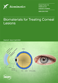
The cornea is a transparent membrane that protects the inner structures of the eye. It is exposed to the external environment and subjected to the risk of lesions and diseases, sometimes resulting in impaired vision and blindness. Several eye pathologies can be treated with keratoplasty, a surgical procedure aimed at replacing the cornea with tissues from human donors. Alternatively, keratoprosthesis is applied to restore minimal functions of the cornea. Recently, many natural and synthetic biomaterials have been developed as corneal substitutes to restore and replace diseased or injured corneas. This paper reviews the most innovative solutions that have been proposed to regenerate the cornea avoiding the use of donor tissues. View this paper
  • Issues are regarded as officially published after their release is announced to the table of contents alert mailing list.
  • You may sign up for e-mail alerts to receive table of contents of newly released issues.
  • PDF is the official format for papers published in both, html and pdf forms. To view the papers in pdf format, click on the "PDF Full-text" link, and use the free Adobe Reader to open them.
Order results
Result details
Section
Select all
Export citation of selected articles as:
20 pages, 9881 KiB  
Article
Review of Vision-Based Environmental Perception for Lower-Limb Exoskeleton Robots
by Chen Wang, Zhongcai Pei, Yanan Fan, Shuang Qiu and Zhiyong Tang
Biomimetics 2024, 9(4), 254; https://doi.org/10.3390/biomimetics9040254 - 22 Apr 2024
Viewed by 1376
Abstract
The exoskeleton robot is a wearable electromechanical device inspired by animal exoskeletons. It combines technologies such as sensing, control, information, and mobile computing, enhancing human physical abilities and assisting in rehabilitation training. In recent years, with the development of visual sensors and deep [...] Read more.
The exoskeleton robot is a wearable electromechanical device inspired by animal exoskeletons. It combines technologies such as sensing, control, information, and mobile computing, enhancing human physical abilities and assisting in rehabilitation training. In recent years, with the development of visual sensors and deep learning, the environmental perception of exoskeletons has drawn widespread attention in the industry. Environmental perception can provide exoskeletons with a certain level of autonomous perception and decision-making ability, enhance their stability and safety in complex environments, and improve the human–machine–environment interaction loop. This paper provides a review of environmental perception and its related technologies of lower-limb exoskeleton robots. First, we briefly introduce the visual sensors and control system. Second, we analyze and summarize the key technologies of environmental perception, including related datasets, detection of critical terrains, and environment-oriented adaptive gait planning. Finally, we analyze the current factors limiting the development of exoskeleton environmental perception and propose future directions. Full article
Show Figures

Figure 1

Figure 1
<p>The role of vision in the human–machine–environment loop of lower-limb exoskeletons.</p>
Full article ">Figure 2
<p>Common visual sensors: (<b>a</b>) Philips’ RGB network camera [<a href="#B46-biomimetics-09-00254" class="html-bibr">46</a>]; (<b>b</b>) ZED’s binocular stereo vision camera, the ZED Mini Stereo Camera [<a href="#B47-biomimetics-09-00254" class="html-bibr">47</a>]; (<b>c</b>) Unitree’s LiDAR L1 [<a href="#B48-biomimetics-09-00254" class="html-bibr">48</a>]; (<b>d</b>) Realsense’s depth camera, the D435i [<a href="#B49-biomimetics-09-00254" class="html-bibr">49</a>]; (<b>e</b>) Realsense’s LiDAR camera, the L515 [<a href="#B45-biomimetics-09-00254" class="html-bibr">45</a>].</p>
Full article ">Figure 3
<p>The role and relationship of controllers at different levels.</p>
Full article ">Figure 4
<p>Stair-line detection methods based on traditional image processing.</p>
Full article ">Figure 5
<p>Illustration of StairNet with RGB-D inputs and StairNet with RGB input and depth estimation.</p>
Full article ">Figure 6
<p>Process of plane-based stair detection methods.</p>
Full article ">Figure 7
<p>The main process of environment-oriented adaptive gait-planning methods, where <math display="inline"><semantics> <mrow> <mi>F</mi> <mo>(</mo> <mi>H</mi> <mo>,</mo> <mi>W</mi> <mo>,</mo> <msub> <mi>l</mi> <mn>1</mn> </msub> <mo>,</mo> <msub> <mi>l</mi> <mn>2</mn> </msub> <mo>,</mo> <mi>T</mi> <mo>)</mo> </mrow> </semantics></math> represents the fitted joint spatio-temporal domain equation, and <span class="html-italic">H</span> and <span class="html-italic">W</span> represent the width and height of the stairs, respectively. <math display="inline"><semantics> <msub> <mi>l</mi> <mn>1</mn> </msub> </semantics></math> and <math display="inline"><semantics> <msub> <mi>l</mi> <mn>2</mn> </msub> </semantics></math> represent the thigh length and calf length, respectively. <span class="html-italic">T</span> represents the gait period. <math display="inline"><semantics> <mrow> <msup> <mi>τ</mi> <mn>2</mn> </msup> <mover accent="true"> <mi>y</mi> <mo>¨</mo> </mover> <mo>=</mo> <msub> <mi>α</mi> <mi>y</mi> </msub> <mrow> <mo>(</mo> <msub> <mi>β</mi> <mi>y</mi> </msub> <mrow> <mo>(</mo> <mi>g</mi> <mo>−</mo> <mi>y</mi> <mo>)</mo> </mrow> <mo>−</mo> <mi>τ</mi> <mover accent="true"> <mi>y</mi> <mo>˙</mo> </mover> <mo>)</mo> </mrow> <mo>+</mo> <mi>f</mi> </mrow> </semantics></math> represents the basic formula of a DMP. <span class="html-italic">y</span> represents the system status, and <math display="inline"><semantics> <mover accent="true"> <mi>y</mi> <mo>˙</mo> </mover> </semantics></math> and <math display="inline"><semantics> <mover accent="true"> <mi>y</mi> <mo>¨</mo> </mover> </semantics></math> represent the first and second derivatives of <span class="html-italic">y</span>, respectively. <span class="html-italic">g</span> represents the target status, <math display="inline"><semantics> <msub> <mi>α</mi> <mi>y</mi> </msub> </semantics></math> and <math display="inline"><semantics> <msub> <mi>β</mi> <mi>y</mi> </msub> </semantics></math> are two constants, <span class="html-italic">f</span> is the forcing term, and <math display="inline"><semantics> <mi>τ</mi> </semantics></math> is the scale factor.</p>
Full article ">
12 pages, 6225 KiB  
Article
Biomineralization of Polyelectrolyte-Functionalized Electrospun Fibers: Optimization and In Vitro Validation for Bone Applications
by Ahmed Salama, Emad Tolba, Ahmed K. Saleh, Iriczalli Cruz-Maya, Marco A. Alvarez-Perez and Vincenzo Guarino
Biomimetics 2024, 9(4), 253; https://doi.org/10.3390/biomimetics9040253 - 22 Apr 2024
Viewed by 1019
Abstract
In recent years, polyelectrolytes have been successfully used as an alternative to non-collagenous proteins to promote interfibrillar biomineralization, to reproduce the spatial intercalation of mineral phases among collagen fibrils, and to design bioinspired scaffolds for hard tissue regeneration. Herein, hybrid nanofibers were fabricated [...] Read more.
In recent years, polyelectrolytes have been successfully used as an alternative to non-collagenous proteins to promote interfibrillar biomineralization, to reproduce the spatial intercalation of mineral phases among collagen fibrils, and to design bioinspired scaffolds for hard tissue regeneration. Herein, hybrid nanofibers were fabricated via electrospinning, by using a mixture of Poly ɛ-caprolactone (PCL) and cationic cellulose derivatives, i.e., cellulose-bearing imidazolium tosylate (CIMD). The obtained fibers were self-assembled with Sodium Alginate (SA) by polyelectrolyte interactions with CIMD onto the fiber surface and, then, treated with simulated body fluid (SBF) to promote the precipitation of calcium phosphate (CaP) deposits. FTIR analysis confirmed the presence of SA and CaP, while SEM equipped with EDX analysis mapped the calcium phosphate constituent elements, estimating an average Ca/P ratio of about 1.33—falling in the range of biological apatites. Moreover, in vitro studies have confirmed the good response of mesenchymal cells (hMSCs) on biomineralized samples, since day 3, with a significant improvement in the presence of SA, due to the interaction of SA with CaP deposits. More interestingly, after a decay of metabolic activity on day 7, a relevant increase in cell proliferation can be recognized, in agreement with the beginning of the differentiation phase, confirmed by ALP results. Antibacterial tests performed by using different bacteria populations confirmed that nanofibers with an SA-CIMD complex show an optimal inhibitory response against S. mutans, S. aureus, and E. coli, with no significant decay due to the effect of CaP, in comparison with non-biomineralized controls. All these data suggest a promising use of these biomineralized fibers as bioinspired membranes with efficient antimicrobial and osteoconductive cues suitable to support bone healing/regeneration. Full article
(This article belongs to the Special Issue Biomimetic Approaches in Healthcare—Innovations Inspired by Nature)
Show Figures

Figure 1

Figure 1
<p>FT-IR spectroscopy of PCL, PCL/CIMD, and PCL/CIMD/SA before (<b>A</b>,<b>C</b>,<b>E</b>) and after calcium phosphate mineralization (<b>B</b>,<b>D</b>,<b>F</b>), respectively. Gray strips highlighted the main characteristic peaks for CIMD and Phosphate groups.</p>
Full article ">Figure 2
<p>Surface morphology after calcium phosphate mineralization of neat PCL (<b>A</b>,<b>B</b>), PCL/CIMD (<b>C</b>,<b>D</b>), and PCL/CIMD/SA (<b>E</b>,<b>F</b>).</p>
Full article ">Figure 3
<p>Elemental mapping via EDX for (<b>A</b>) PCL/CIMD/SA and (<b>B</b>) PCL/CIMD/SA/CP: Carbon (Red), Nitrogel (Green), Sulfur (Blue); Oxygen (Cyan), Phosphorus (Yellow), and Calcium (Orange).</p>
Full article ">Figure 3 Cont.
<p>Elemental mapping via EDX for (<b>A</b>) PCL/CIMD/SA and (<b>B</b>) PCL/CIMD/SA/CP: Carbon (Red), Nitrogel (Green), Sulfur (Blue); Oxygen (Cyan), Phosphorus (Yellow), and Calcium (Orange).</p>
Full article ">Figure 4
<p>In vitro studies of biocompatibility: (<b>A</b>) Adhesion of cells, calculated with respect to tissue culture plate (TCP). Significant differences are represented as * <span class="html-italic">p</span> &lt; 0.05. SEM images of hMSCs after 24 h in cell culture with PCL/CP (<b>B</b>), PCL/CIMD/CP (<b>C</b>), and PCL/CIMD/SA/CP (<b>D</b>) nanofibers.</p>
Full article ">Figure 5
<p>In vitro Viability (XTT tests): hMSC response for 14 days on PCL, PCL/CIMD, and PCL/CIMD/SA after biomineralization. Data were reported as mean ± standard error deviation (* <span class="html-italic">p</span> &lt; 0.05, ** <span class="html-italic">p</span> &lt; 0.01, *** <span class="html-italic">p</span> &lt; 0.001).</p>
Full article ">Figure 6
<p>ALP activity of hMSCs after 3 and 7 days of culture onto the tissue culture plate (TCP), PCL, PCL/CP, PCL/CIMD/CP, and PCL/CIMD/SA/CP fibers. (* <span class="html-italic">p</span> &lt; 0.05, ** <span class="html-italic">p</span> &lt; 0.01, *** <span class="html-italic">p</span> &lt; 0.001).</p>
Full article ">Figure 7
<p>Antimicrobial tests by halo-zone expression, against four different strains. PCL/CP, PCL/CIMD/CP, and PCL/CIMD/SA/CP were coded as 1, 2, and 3, respectively.</p>
Full article ">
17 pages, 20940 KiB  
Article
Strontium and Copper Co-Doped Multifunctional Calcium Phosphates: Biomimetic and Antibacterial Materials for Bone Implants
by Vladimir N. Lebedev, Mariya I. Kharovskaya, Bogdan I. Lazoryak, Anastasiya O. Solovieva, Inna V. Fadeeva, Abdulkarim A. Amirov, Maksim A. Koliushenkov, Farid F. Orudzhev, Oksana V. Baryshnikova, Viktoriya G. Yankova, Julietta V. Rau and Dina V. Deyneko
Biomimetics 2024, 9(4), 252; https://doi.org/10.3390/biomimetics9040252 - 20 Apr 2024
Viewed by 1526
Abstract
β-tricalcium phosphate (β-TCP) is a promising material in regenerative traumatology for the creation of bone implants. Previously, it was established that doping the structure with certain cations can reduce the growth of bacterial activity. Recently, much attention has been paid to co-doped β-TCP, [...] Read more.
β-tricalcium phosphate (β-TCP) is a promising material in regenerative traumatology for the creation of bone implants. Previously, it was established that doping the structure with certain cations can reduce the growth of bacterial activity. Recently, much attention has been paid to co-doped β-TCP, that is explained by their ability, on the one hand, to reduce cytotoxicity for cells of the human organism, on the other hand, to achieve a successful antibacterial effect. Sr, Cu-co-doped solid solutions of the composition Ca9.5–xSrxCu(PO4)7 was obtained by the method of solid-phase reactions. The Rietveld method of structural refinement revealed the presence of Sr2+ ions in four crystal sites: M1, M2, M3, and M4. The M5 site is completely occupied by Cu2+. Isomorphic substitution of Ca2+ → (Sr2+and Cu2+) expands the concentration limits of the existence of the solid solution with the β-TCP structure. No additional phases were formed up to x = 4.5 in Ca9.5–xSrxCu(PO4)7. Biocompatibility tests were performed on cell lines of human bone marrow mesenchymal stromal cells (hMSC), human fibroblasts (MRC-5) and osteoblasts (U-2OS). It was demonstrated that cytotoxicity exhibited a concentration dependence, along with an increase in osteogenesis and cell proliferation. Ca9.5–xSrxCu(PO4)7 powders showed significant inhibitory activity against pathogenic strains Escherichia coli and Staphylococcus aureus. Piezoelectric properties of Ca9.5–xSrxCu(PO4)7 were investigated. Possible ways to achieve high piezoelectric response are discussed. The combination of bioactive properties of Ca9.5–xSrxCu(PO4)7 renders them multifunctional materials suitable for bone substitutes. Full article
(This article belongs to the Special Issue Advances in Bioceramics for Bone Regeneration)
Show Figures

Figure 1

Figure 1
<p>The sequence of research on biological cell cultures. Created with <a href="http://BioRender.com" target="_blank">BioRender.com</a>.</p>
Full article ">Figure 2
<p>PXRD patterns of Ca<sub>9.5–<span class="html-italic">x</span></sub>Sr<span class="html-italic"><sub>x</sub></span>Cu(PO<sub>4</sub>)<sub>7</sub> with 0 ≤ <span class="html-italic">x</span> ≤ 4.5 (<b>a</b>). Shifting of the main diffraction reflections in Ca<sub>9.5–<span class="html-italic">x</span></sub>Sr<span class="html-italic"><sub>x</sub></span>Cu(PO<sub>4</sub>)<sub>7</sub>, 0 ≤ <span class="html-italic">x</span> ≤ 4.5 (<b>b</b>).</p>
Full article ">Figure 3
<p>The dependence of the unit cell parameters <span class="html-italic">a</span> and <span class="html-italic">c</span> for Ca<sub>9.5–<span class="html-italic">x</span></sub>Sr<span class="html-italic"><sub>x</sub></span>Cu(PO<sub>4</sub>)<sub>7</sub> solid solutions.</p>
Full article ">Figure 4
<p>FT-IR spectra of Ca<sub>9.5–<span class="html-italic">x</span></sub>Sr<span class="html-italic"><sub>x</sub></span>Cu(PO<sub>4</sub>)<sub>7</sub> with 0 ≤ <span class="html-italic">x</span> ≤ 2 (<b>a</b>) and 2 ≤ <span class="html-italic">x</span> ≤ 4.5 (<b>b</b>).</p>
Full article ">Figure 5
<p>The dependence of the occupation site on the composition Ca<sub>9.5–<span class="html-italic">x</span></sub>Sr<span class="html-italic"><sub>x</sub></span>Cu(PO<sub>4</sub>)<sub>7</sub> (<b>a</b>). The fragment of structure Ca<sub>8.5</sub>SrCu(PO<sub>4</sub>)<sub>7</sub> (<b>b</b>).</p>
Full article ">Figure 6
<p>The accumulative release amount of Ca<sup>2+</sup>, Cu<sup>2+</sup> and Sr<sup>2+</sup> ions from Ca<sub>9.5</sub>Cu(PO<sub>4</sub>)<sub>7</sub> (<b>a</b>) and Ca<sub>5</sub>Sr<sub>4.5</sub>Cu(PO<sub>4</sub>)<sub>7</sub> (<b>b</b>) samples after soaking in Tris-HCl buffer solution for 4, 7, 14 and 18 days.</p>
Full article ">Figure 7
<p>Viability of hMSCs cells after cultivation on a powder layer of Ca<sub>9.5</sub>Cu(PO<sub>4</sub>)<sub>7</sub> and Ca<sub>5</sub>Sr<sub>4.5</sub>Cu(PO<sub>4</sub>)<sub>7</sub> samples (<b>a</b>). Viability of MRC-5 and hMSCs while adding ceramic powders to cell medium for 3 days (magnification ×20) (<b>b</b>).</p>
Full article ">Figure 8
<p>Viability of hMSCs cells after cultivation on a powder layer of Ca<sub>5</sub>Sr<sub>4.5</sub>Cu(PO<sub>4</sub>)<sub>7</sub> (magnification ×20).</p>
Full article ">Figure 9
<p>The cytotoxicity of the solution derived from Ca<sub>9.5</sub>Cu(PO<sub>4</sub>)<sub>7</sub> and Ca<sub>5</sub>Sr<sub>4.5</sub>Cu(PO<sub>4</sub>)<sub>7</sub> powders on hMSCs cells (<b>a</b>), and U-2 OS cells (<b>b</b>) assessed using the MTT test.</p>
Full article ">Figure 10
<p>The inhibition of bacteria (<span class="html-italic">E. coli</span> and <span class="html-italic">S. aureus</span>) grown for 24 h in the presence of Ca<sub>9.5–<span class="html-italic">x</span></sub>Sr<span class="html-italic"><sub>x</sub></span>Cu(PO<sub>4</sub>)<sub>7</sub>. The positive control (ctr) is represented by the growth of each bacteria strain in the absence of phosphates.</p>
Full article ">Figure 11
<p>AFM images of Ca<sub>9</sub>Sr<sub>0.5</sub>Cu(PO<sub>4</sub>)<sub>7</sub> sample: (<b>a</b>) 2D AFM map, (<b>b</b>) 3D AFM map.</p>
Full article ">Figure 12
<p>PFM images of Ca<sub>9</sub>Sr<sub>0.5</sub>Cu(PO<sub>4</sub>)<sub>7</sub> sample: amplitude (<b>a</b>,<b>c</b>) and phase (<b>b</b>,<b>d</b>) in vertical (<b>a</b>,<b>b</b>) and horizontal (<b>c</b>,<b>d</b>) modes.</p>
Full article ">
16 pages, 9892 KiB  
Article
Effects of Sodium Alginate and Calcium Chloride on Fungal Growth and Viability in Biomass-Fungi Composite Materials Used for 3D Printing
by Al Mazedur Rahman, Caleb Oliver Bedsole, Yeasir Mohammad Akib, Jillian Hamilton, Taieba Tuba Rahman, Brian D. Shaw and Zhijian Pei
Biomimetics 2024, 9(4), 251; https://doi.org/10.3390/biomimetics9040251 - 20 Apr 2024
Cited by 1 | Viewed by 1488
Abstract
To combat climate change, one approach is to manufacture products from biomass-fungi composite materials instead of petroleum-based plastics. These products can be used in packaging, furniture, and construction industries. A 3D printing-based manufacturing method was developed for these biomass-fungi composite materials, eliminating the [...] Read more.
To combat climate change, one approach is to manufacture products from biomass-fungi composite materials instead of petroleum-based plastics. These products can be used in packaging, furniture, and construction industries. A 3D printing-based manufacturing method was developed for these biomass-fungi composite materials, eliminating the need for molds, and enabling customized product design. However, previous studies on the 3D printing-based method showed significant shrinkage of printed samples. In this paper, an approach is proposed to reduce the shrinkage by incorporating ionic crosslinking into biomass-fungi composite materials. This paper reports two sets of experiments regarding the effects of sodium alginate (SA) and calcium chloride (CaCl2) on fungal growth and fungal viability. The first set of experiments was conducted using Petri dishes with fungi isolated from colonized biomass-fungi material and different concentrations of SA and CaCl2. Fungal growth was measured by the circumference of fungal colonies. The results showed that concentrations of SA and CaCl2 had significant effects on fungal growth and no fungal growth was observed on Petri dishes with 15% CaCl2. Some of these Petri dishes were also observed under confocal microscopy. The results confirmed the differences obtained by measuring the circumference of fungal colonies. The second set of experiments was conducted using Petri dishes with biomass-fungi mixtures that were treated with different concentrations of SA and exposure times in a CaCl2 (crosslinking) solution. Fungal viability was measured by counting colony-forming units. The results showed that the addition of the SA solution and exposure times in the crosslinking solution had statistically significant effects on fungal viability. The 2SA solution was prepared by dissolving 2 g of SA in 100 mL of water, the 5SA solution was prepared by dissolving 5 g of SA in 100 mL of water, and the crosslinking solution was prepared by dissolving 5 g of CaCl2 in 100 mL of water. The results also showed that fungal viability was not too low in biomass-fungi mixtures that included 2SA solution and were exposed to the crosslinking solution for 1 min. Full article
Show Figures

Figure 1

Figure 1
<p>Processes of a 3D printing-based manufacturing method using biomass-fungi composite materials.</p>
Full article ">Figure 2
<p>Overview of the experimental procedure for <a href="#sec2-biomimetics-09-00251" class="html-sec">Section 2</a>.</p>
Full article ">Figure 3
<p>Mean values of the circumference of fungal colonies in Petri dishes with different medium solutions.</p>
Full article ">Figure 4
<p>Timelapse images of hypha growth on Petri dishes with different medium solutions (control, 2% SA, and 5% SA), scale bar = 10 μm.</p>
Full article ">Figure 5
<p>Overview of the experimental procedure used in <a href="#sec3-biomimetics-09-00251" class="html-sec">Section 3</a>.</p>
Full article ">Figure 6
<p>Preparation procedure of SA solution with the concentration of 2:100 (2SA) (<span class="html-italic">w</span>/<span class="html-italic">v</span>).</p>
Full article ">Figure 7
<p>Preparation procedure of crosslinking solution with the concentration of 5:100 (<span class="html-italic">w</span>/<span class="html-italic">v</span>).</p>
Full article ">Figure 8
<p>Preparing procedure for plated samples.</p>
Full article ">Figure 9
<p>Colony Forming Units per plate (CFUs/plate) based on different treatments, (<b>a</b>) 0SA vs. 2SA and 5SA without crosslinking plated samples, (<b>b</b>) 2SA and 5SA without crosslinking vs. with crosslinking plated samples.</p>
Full article ">
18 pages, 6194 KiB  
Article
Morphological Reconstruction for Variable Wing Leading Edge Based on the Node Curvature Vectors
by Jie Zeng, Qingfeng Zhu, Yueqi Zhao, Zhigang Wang, Yu Yang, Qi Wu and Jinpeng Cui
Biomimetics 2024, 9(4), 250; https://doi.org/10.3390/biomimetics9040250 - 20 Apr 2024
Viewed by 947
Abstract
Precise morphology acquisition for the variable wing leading edge is essential for its bio-inspired adaptive control. Therefore, this study proposes a morphological reconstruction method for the variable wing leading edge, utilizing the node curvature vectors-based curvature propagation method (NCV-CPM). By establishing a strain–arc [...] Read more.
Precise morphology acquisition for the variable wing leading edge is essential for its bio-inspired adaptive control. Therefore, this study proposes a morphological reconstruction method for the variable wing leading edge, utilizing the node curvature vectors-based curvature propagation method (NCV-CPM). By establishing a strain–arc curvature function, the method fundamentally mitigates the impact of surface curvature angle on curvature computation accuracy at sensing points. We introduce a technique that uses high-order curvature fitting functions to determine the curvature vectors of arc segment nodes. This method reduces cumulative errors in curvature computation linked to the linear interpolation-based curvature propagation method (LI-CPM) at unattached sensor positions. Integrating curvature–strain functions aids in wing leading-edge strain field reconstruction, supporting structural health monitoring. Additionally, a particle swarm algorithm optimizes the sensing point distribution, reducing network complexity. This study demonstrates significantly enhanced morphological reconstruction accuracy compared to those obtained with conventional LI-CPM. Full article
Show Figures

Figure 1

Figure 1
<p>(<b>a</b>) Section selected in the leading edge of the variable wing; (<b>b</b>) comparison of the selected section before and after deformation.</p>
Full article ">Figure 2
<p>Schematic diagram of arc division density optimization.</p>
Full article ">Figure 3
<p>Arc segment node definition.</p>
Full article ">Figure 4
<p>Curvature and strain field reconstruction process based on node curvature vectors.</p>
Full article ">Figure 5
<p>Coordinate increment calculation of arc segment.</p>
Full article ">Figure 6
<p>Number optimization of virtual sensing points based on particle swarm optimization algorithm.</p>
Full article ">Figure 7
<p>The leading edge of the morphing wing.</p>
Full article ">Figure 8
<p>Arc segment division scheme.</p>
Full article ">Figure 9
<p>Comparison of reconstruction results in Path1: (<b>a</b>) curvature result; (<b>b</b>) strain result.</p>
Full article ">Figure 10
<p>The number optimization process of sensing points based on the particle swarm optimization algorithm.</p>
Full article ">Figure 11
<p>Morphological reconstruction results of NCV-CPM for wing leading edge of deflection angle 10°: (<b>a</b>) Euclidean distance cloud map; (<b>b</b>) reconstruction effect comparison.</p>
Full article ">Figure 12
<p>Propagation reconstruction effect comparison of LI-CPM and NCV-CPM: (<b>a</b>) relative error under 10° deflection angle of leading edge; (<b>b</b>) root mean square error under four leading edge deflection angles.</p>
Full article ">Figure 13
<p>(<b>a</b>) Experimental system of wing leading-edge deformation reconstruction; (<b>b</b>) integration between strain sensor and leading edge.</p>
Full article ">Figure 14
<p>Layout scheme of strain-sensing measuring points in staggered complementary mode.</p>
Full article ">Figure 15
<p>Comparison of reconstruction results in Path B: (<b>a</b>) curvature results; (<b>b</b>) strain results.</p>
Full article ">Figure 16
<p>Morphological reconstruction results of NCV-CPM for wing leading edge of deflection at angle of 12°: (<b>a</b>) leading-edge deflection diagram; (<b>b</b>) reconstruction effect comparison.</p>
Full article ">Figure 17
<p>Propagation reconstruction effect comparison of LI-CPM and NCV-CPM: (<b>a</b>) relative error under 12° deflection angle of leading edge; (<b>b</b>) root mean square error under four leading-edge deflection angles.</p>
Full article ">
23 pages, 7969 KiB  
Article
Numerical Simulation of the Advantages of the Figure-Eight Flapping Motion of an Insect on Aerodynamics under Low Reynolds Number Conditions
by Masato Yoshida and Tomohiro Fukui
Biomimetics 2024, 9(4), 249; https://doi.org/10.3390/biomimetics9040249 - 20 Apr 2024
Viewed by 864
Abstract
In proceeding with the advanced development of small unmanned aerial vehicles (UAVs), which are small flying machines, understanding the flight of insects is important because UAVs that use flight are attracting attention. The figure-eight trajectory of the wing tips is often observed in [...] Read more.
In proceeding with the advanced development of small unmanned aerial vehicles (UAVs), which are small flying machines, understanding the flight of insects is important because UAVs that use flight are attracting attention. The figure-eight trajectory of the wing tips is often observed in the flight of insects. In this study, we investigated the more efficient figure-eight motion patterns in generating lift during the hovering motion and the relationship between figure-eight motion and Reynolds number. For this purpose, we compared the ratios of the cycle-averaged lift coefficient to the power coefficient generated from each motion by varying the elevation motion angle, which is the rotational motion that represents the figure-eight motion, and the Reynolds number. The result showed that the motion with a smaller initial phase of the elevation motion angle (φe090°) could generate lift more efficiently at all Reynolds numbers. In addition, the figure-eight motion was more effective when the Reynolds number was low. Full article
(This article belongs to the Special Issue Bio-Inspired Design and Control of Unmanned Aerial Vehicles (UAVs))
Show Figures

Figure 1

Figure 1
<p>Computational model of an (<b>a</b>) insect and (<b>b</b>) wing. Only the two wings shown in gray were analyzed without body reproduction. The red line represents the wing length.</p>
Full article ">Figure 2
<p>Definition of the flapping motion of the insect in (<b>a</b>) bird’s eye view, (<b>b</b>) <math display="inline"><semantics> <mrow> <mi>x</mi> <mo>–</mo> <mi>z</mi> </mrow> </semantics></math> plane, and (<b>c</b>) <math display="inline"><semantics> <mrow> <mi>y</mi> <mo>–</mo> <mi>z</mi> </mrow> </semantics></math> plane. The wings, which are the analysis objects, are shown in gray. On the other hand, the body, which is not the analysis object, is shown by the dotted line.</p>
Full article ">Figure 3
<p>Representation of insect flapping motion. (<b>a</b>) Time history of the positional angle, feathering angle, and elevation angle. (<b>b</b>) Trajectory of wing tips. In <a href="#biomimetics-09-00249-f003" class="html-fig">Figure 3</a><b>b</b>,The gray solid and dotted lines represent the trajectory of the wings tips and the body of the insect, respectively.</p>
Full article ">Figure 4
<p>3D27V model for the three-dimensional lattice Boltzmann method. The numbers (0~26) represent the 27 directions of the 3D27Vmodel.</p>
Full article ">Figure 5
<p>Virtual boundary points. The gray and white areas represent the interior of the object and fluid, respectively.</p>
Full article ">Figure 6
<p>Schematic view of the physical quantity calculation method at the virtual boundary point. The gray and white areas represent the interior of the object and fluid, respectively.</p>
Full article ">Figure 7
<p>Schematic view of the computational model: (<b>a</b>) bird’s eye view, (<b>b</b>) <math display="inline"><semantics> <mrow> <mi>x</mi> <mo>–</mo> <mi>z</mi> </mrow> </semantics></math> plane, and (<b>c</b>) <math display="inline"><semantics> <mrow> <mi>x</mi> <mo>–</mo> <mi>y</mi> </mrow> </semantics></math> plane. The representative length <math display="inline"><semantics> <mrow> <mi>L</mi> </mrow> </semantics></math> is the mean chord length <math display="inline"><semantics> <mrow> <msub> <mrow> <mi>C</mi> </mrow> <mrow> <mi>m</mi> </mrow> </msub> </mrow> </semantics></math> shown in <a href="#sec2dot1-biomimetics-09-00249" class="html-sec">Section 2.1</a>. In <a href="#biomimetics-09-00249-f007" class="html-fig">Figure 7</a><b>a</b>, the wings and grid model are shown in green and black or gray lines, respectively. In <a href="#biomimetics-09-00249-f007" class="html-fig">Figure 7</a><b>b</b>,<b>c</b>, the wings are shown in gray areas, and block areas of grid model consisting of different grid sizes are represented by black, green, red, and blue lines.</p>
Full article ">Figure 8
<p>Time history of the lift coefficient in seven cycles with <math display="inline"><semantics> <mrow> <mi>U</mi> <mo>=</mo> <mn>0.04</mn> </mrow> </semantics></math>.</p>
Full article ">Figure 9
<p>Time history of the (<b>a</b>) lift coefficient, (<b>b</b>) pressure component of lift coefficient, and (<b>c</b>) viscous stress component of lift coefficient for three resolutions.</p>
Full article ">Figure 10
<p>Schematic view of the movement of an oscillating plate.</p>
Full article ">Figure 11
<p>Time history of the lift coefficient of an oscillating plate. The result was compared with those of Trizila [<a href="#B36-biomimetics-09-00249" class="html-bibr">36</a>] and Wang et al. [<a href="#B37-biomimetics-09-00249" class="html-bibr">37</a>].</p>
Full article ">Figure 12
<p>Trajectory of the wing tip in each motion. (<b>a</b>) With figure-eight motion and (<b>b</b>) without figure-eight motion. The gray line represents the trajectory of the wing tip.</p>
Full article ">Figure 13
<p>Vortex structures and normalized helicity density over one stroke cycle for each motion. (<b>a</b>) With and (<b>b</b>) without figure-eight motions at <math display="inline"><semantics> <mrow> <mi>t</mi> <mo>=</mo> <mn>0.25</mn> <mi>T</mi> </mrow> </semantics></math>; (<b>c</b>) with and (<b>d</b>) without figure-eight motions at <math display="inline"><semantics> <mrow> <mi>t</mi> <mo>=</mo> <mn>0.50</mn> <mi>T</mi> </mrow> </semantics></math>; (<b>e</b>) with and (<b>f</b>) without figure-eight motions at <math display="inline"><semantics> <mrow> <mi>t</mi> <mo>=</mo> <mn>0.75</mn> <mi>T</mi> </mrow> </semantics></math>; and (<b>g</b>) with and (<b>h</b>) without figure-eight motions at <math display="inline"><semantics> <mrow> <mi>t</mi> <mo>=</mo> <mn>1.00</mn> <mi>T</mi> </mrow> </semantics></math>.</p>
Full article ">Figure 14
<p>Time histories of (<b>a</b>) lift coefficient, (<b>b</b>) thrust coefficient, and (<b>c</b>) power coefficient over one stroke cycle for each motion.</p>
Full article ">Figure 15
<p>Vortex structures (<math display="inline"><semantics> <mrow> <msup> <mrow> <mi>Q</mi> </mrow> <mrow> <mo>∗</mo> </mrow> </msup> <mo>=</mo> <mn>0.8</mn> </mrow> </semantics></math>) and normalized pressure coefficient for each motion in the downstroke at <math display="inline"><semantics> <mrow> <mi>t</mi> <mo>=</mo> <mn>0.1</mn> <mi>T</mi> </mrow> </semantics></math>. Vortex structures (<math display="inline"><semantics> <mrow> <msup> <mrow> <mi>Q</mi> </mrow> <mrow> <mo>∗</mo> </mrow> </msup> <mo>=</mo> <mn>0.8</mn> </mrow> </semantics></math>) and normalized pressure coefficients from (<b>a</b>) with and (<b>b</b>) without figure-eight motions. Normalized pressure coefficient at the wing tip from (<b>c</b>) with and (<b>d</b>) without figure-eight motions.</p>
Full article ">Figure 16
<p>Trajectory of the wing tip in each motion: (<b>a</b>) <math display="inline"><semantics> <mrow> <msub> <mrow> <mi>φ</mi> </mrow> <mrow> <mi>e</mi> <mn>0</mn> </mrow> </msub> <mo>=</mo> <mn>0</mn> <mo>°</mo> </mrow> </semantics></math>, (<b>b</b>) <math display="inline"><semantics> <mrow> <msub> <mrow> <mi>φ</mi> </mrow> <mrow> <mi>e</mi> <mn>0</mn> </mrow> </msub> <mo>=</mo> <mn>45</mn> <mo>°</mo> </mrow> </semantics></math>; (<b>c</b>) <math display="inline"><semantics> <mrow> <msub> <mrow> <mi>φ</mi> </mrow> <mrow> <mi>e</mi> <mn>0</mn> </mrow> </msub> <mo>=</mo> <mn>90</mn> <mo>°</mo> </mrow> </semantics></math>; (<b>d</b>) <math display="inline"><semantics> <mrow> <msub> <mrow> <mi>φ</mi> </mrow> <mrow> <mi>e</mi> <mn>0</mn> </mrow> </msub> <mo>=</mo> <mn>135</mn> <mo>°</mo> </mrow> </semantics></math>; (<b>e</b>) <math display="inline"><semantics> <mrow> <msub> <mrow> <mi>φ</mi> </mrow> <mrow> <mi>e</mi> <mn>0</mn> </mrow> </msub> <mo>=</mo> <mn>180</mn> <mo>°</mo> </mrow> </semantics></math>; (<b>f</b>) <math display="inline"><semantics> <mrow> <msub> <mrow> <mi>φ</mi> </mrow> <mrow> <mi>e</mi> <mn>0</mn> </mrow> </msub> <mo>=</mo> <mn>225</mn> <mo>°</mo> </mrow> </semantics></math>; (<b>g</b>) <math display="inline"><semantics> <mrow> <msub> <mrow> <mi>φ</mi> </mrow> <mrow> <mi>e</mi> <mn>0</mn> </mrow> </msub> <mo>=</mo> <mn>270</mn> <mo>°</mo> </mrow> </semantics></math>; and (<b>h</b>) <math display="inline"><semantics> <mrow> <msub> <mrow> <mi>φ</mi> </mrow> <mrow> <mi>e</mi> <mn>0</mn> </mrow> </msub> <mo>=</mo> <mn>315</mn> <mo>°</mo> </mrow> </semantics></math>. The gray line represents the trajectory of the wing tip.</p>
Full article ">Figure 17
<p>Relation between the cycle-averaged lift coefficient and power coefficient for each motion at each Reynolds number. (<b>a</b>) <math display="inline"><semantics> <mrow> <mi>R</mi> <mi>e</mi> <mo>=</mo> <mn>33.5</mn> </mrow> </semantics></math>; (<b>b</b>) <math display="inline"><semantics> <mrow> <mi>R</mi> <mi>e</mi> <mo>=</mo> <mn>67</mn> </mrow> </semantics></math>; (<b>c</b>) <math display="inline"><semantics> <mrow> <mi>R</mi> <mi>e</mi> <mo>=</mo> <mn>134</mn> </mrow> </semantics></math>; (<b>d</b>) <math display="inline"><semantics> <mrow> <mi>R</mi> <mi>e</mi> <mo>=</mo> <mn>268</mn> </mrow> </semantics></math>; (<b>e</b>) <math display="inline"><semantics> <mrow> <mi>R</mi> <mi>e</mi> <mo>=</mo> <mn>546</mn> </mrow> </semantics></math>; (<b>f</b>) all Reynolds numbers. Light blue areas shown in the figure (<span class="html-fig-inline" id="biomimetics-09-00249-i001"><img alt="Biomimetics 09 00249 i001" src="/biomimetics/biomimetics-09-00249/article_deploy/html/images/biomimetics-09-00249-i001.png"/></span>) indicate more efficiency than without figure-eight motions.</p>
Full article ">Figure 18
<p>Relation between the initial phase of elevation angle of the most efficient motion in generating lift and Reynolds number.</p>
Full article ">Figure 19
<p>Schematic view of the elliptic approximation.</p>
Full article ">Figure 20
<p>Relation between the aspect ratio and Reynolds number.</p>
Full article ">
17 pages, 2830 KiB  
Review
Exploring Embodied Intelligence in Soft Robotics: A Review
by Zikai Zhao, Qiuxuan Wu, Jian Wang, Botao Zhang, Chaoliang Zhong and Anton A. Zhilenkov
Biomimetics 2024, 9(4), 248; https://doi.org/10.3390/biomimetics9040248 - 19 Apr 2024
Viewed by 1848
Abstract
Soft robotics is closely related to embodied intelligence in the joint exploration of the means to achieve more natural and effective robotic behaviors via physical forms and intelligent interactions. Embodied intelligence emphasizes that intelligence is affected by the synergy of the brain, body, [...] Read more.
Soft robotics is closely related to embodied intelligence in the joint exploration of the means to achieve more natural and effective robotic behaviors via physical forms and intelligent interactions. Embodied intelligence emphasizes that intelligence is affected by the synergy of the brain, body, and environment, focusing on the interaction between agents and the environment. Under this framework, the design and control strategies of soft robotics depend on their physical forms and material properties, as well as algorithms and data processing, which enable them to interact with the environment in a natural and adaptable manner. At present, embodied intelligence has comprehensively integrated related research results on the evolution, learning, perception, decision making in the field of intelligent algorithms, as well as on the behaviors and controls in the field of robotics. From this perspective, the relevant branches of the embodied intelligence in the context of soft robotics were studied, covering the computation of embodied morphology; the evolution of embodied AI; and the perception, control, and decision making of soft robotics. Moreover, on this basis, important research progress was summarized, and related scientific problems were discussed. This study can provide a reference for the research of embodied intelligence in the context of soft robotics. Full article
(This article belongs to the Special Issue Bio-Inspired and Biomimetic Intelligence in Robotics)
Show Figures

Figure 1

Figure 1
<p>PRISMA diagram of literature search [<a href="#B10-biomimetics-09-00248" class="html-bibr">10</a>].</p>
Full article ">Figure 2
<p>This figure, generated from the annual count of eligible papers, illustrates the growth trend of embodied intelligence in soft robotics over several years.</p>
Full article ">Figure 3
<p>Multilayered and interactive map of diverse intelligence systems.</p>
Full article ">Figure 4
<p>(<b>a</b>) Aurelia-inspired robot based on SMA artificial muscle [<a href="#B24-biomimetics-09-00248" class="html-bibr">24</a>]. (<b>b</b>) Sea turtle-inspired swimming robot [<a href="#B25-biomimetics-09-00248" class="html-bibr">25</a>]. (<b>c</b>) Bionic soft robotic fish investigates deep-sea environments [<a href="#B26-biomimetics-09-00248" class="html-bibr">26</a>]; reproduced with permission from ref. [<a href="#B26-biomimetics-09-00248" class="html-bibr">26</a>], copyright 2023, Springer Nature.</p>
Full article ">Figure 5
<p>(<b>a</b>) General reservoir computing, also known as an echo state network, is considered as an extension framework of neural networks. It shares the same three-layer structure. (<b>b</b>) Mass-spring networks are a biomimetic computing model. (<b>c</b>) Sampled modular pneumatic soft arm as an energy storage reservoir.</p>
Full article ">Figure 6
<p>(<b>a</b>) Evolution of intelligent agents in different terrains. Reproduced with permission from ref. [<a href="#B42-biomimetics-09-00248" class="html-bibr">42</a>], copyright 2021, Springer Nature. (<b>b</b>) Each row depicts a different evolved robot moving from left to right. Voxels in the figure are colored based on the amount of subsequent morphological development remaining in that cell: blue indicates shrinking voxels, red indicates growing voxels, and green indicates minimal change. The first row features an evolved soft quadrupedal robot trotting with a two-beat gait synchronizing diagonal pairs of legs. The second row shows an adult robot galloping at full speed (fully airborne mid-gait). The third row depicts a juvenile robot galloping at full speed, evolving into an adult form capable of rolling. The fourth row showcases a rolling robot. Reproduced with permission from ref. [<a href="#B44-biomimetics-09-00248" class="html-bibr">44</a>], copyright 2018, Springer Nature.</p>
Full article ">Figure 7
<p>(<b>a</b>) <span class="html-italic">Dictyostelium discoideum</span>, commonly referred to as slime mold, capable of a transition from a collection of unicellular amoebae into a multicellular organism [<a href="#B46-biomimetics-09-00248" class="html-bibr">46</a>]; (<b>b</b>) modular reconfigurable robots [<a href="#B47-biomimetics-09-00248" class="html-bibr">47</a>]. Reproduced with permission from ref. [<a href="#B47-biomimetics-09-00248" class="html-bibr">47</a>], copyright 2022, Springer Nature.</p>
Full article ">Figure 8
<p>(<b>a</b>) Soft-bodied biomimetic robotic fish. (<b>b</b>) A schematic diagram of reinforcement learning-based control. The environment frames captured by the camera at a speed of 60 fps are sent to DeepLabCut for pose estimation to obtain the precise position and posture of the robotic fish. This precise position and posture information is then used as input for the reinforcement learning algorithm to train the soft-bodied biomimetic robotic fish to reach the target [<a href="#B54-biomimetics-09-00248" class="html-bibr">54</a>]; reproduced with permission from ref. [<a href="#B54-biomimetics-09-00248" class="html-bibr">54</a>], copyright 2023, Springer Nature.</p>
Full article ">
18 pages, 52434 KiB  
Article
Biomimetic Ultrasonic Vibrator with Broadband Characteristics Inspired by Leaf-Cutting Ants
by Wenshuai Wu, Guang Yao, Mingshuo Zhang, Xinggang Jiang and Deyuan Zhang
Biomimetics 2024, 9(4), 247; https://doi.org/10.3390/biomimetics9040247 - 19 Apr 2024
Viewed by 1139
Abstract
Power ultrasound is widely used in industrial production, medical equipment, aerospace, and other fields. Currently, there are two main types of commonly used power generation devices: piezoelectric ultrasonic transducers and magnetostrictive ultrasonic transducers. However, in certain situations with limited external dimensions, the applications [...] Read more.
Power ultrasound is widely used in industrial production, medical equipment, aerospace, and other fields. Currently, there are two main types of commonly used power generation devices: piezoelectric ultrasonic transducers and magnetostrictive ultrasonic transducers. However, in certain situations with limited external dimensions, the applications of existing power ultrasound devices are limited. In nature, leaf-cutting ants excite vibrations through their tiny organs. Inspired by the vibratory organs of leaf-cutting ants, a new type of biomimetic ultrasonic vibrator (BUV) comprising a scraper, dentate disc, and fixture system was proposed, fabricated, and tested in this study. The experimental results showed that the BUV could operate in the frequency range of 16.8–19 kHz. Within the working frequency range, the vibration of the BUV was stable and the amplitude of the vibration displacement was greater than 22 µm. The operating frequency band of the BUV was broader than those of the piezoelectric and magnetostrictive ultrasonic transducers. In addition, the BUV can cut soft rubber and pig tissues with sufficient output power and load-carrying capacity. The BUV, as a new type of power ultrasonic excitation device, is expected to be applied in high-power micro operating scenarios, such as minimally invasive surgical instruments. Full article
Show Figures

Figure 1

Figure 1
<p>Leaf cutting ant and excitation organs. (<b>a</b>) <span class="html-italic">Atta cephalotes</span>, (<b>b</b>) excitation organs of leaf-cutting ant, (<b>c</b>) the file and teeth, (<b>d</b>) the tip of the scraper, (<b>e</b>,<b>f</b>) Structure diagram of excitation organs.</p>
Full article ">Figure 2
<p>BUV. (<b>a</b>) Structure of BUV, (<b>b</b>) part drawing of the scraper, (<b>c</b>) the scraper and teeth of the dentate disc.</p>
Full article ">Figure 3
<p>Contact and engage relationship between scraper and dentate disc (<b>a</b>,<b>b</b>).</p>
Full article ">Figure 4
<p>Contact and engage relationship between the scraper and dentate disc.</p>
Full article ">Figure 5
<p>Vibration model. (<b>a</b>) A simplified model of the BUV, (<b>b</b>) lumped-parameter model, (<b>c</b>) equivalent model of lumped-parameter model, (<b>d</b>) amplitude–frequency characteristics of the equivalent model.</p>
Full article ">Figure 6
<p>Experimental platform and simulation model. (<b>a</b>) Experimental platform, (<b>b</b>) finite element model of the BUV, (<b>c</b>) finite element model for harmonic analysis of the scraper, (<b>d</b>) load-carrying capacity test.</p>
Full article ">Figure 7
<p>Harmonic response and the operational frequency band. (<b>a</b>) Harmonic response of the Sa scraper, (<b>b</b>) harmonic response of the Sb scraper, (<b>c</b>) operational frequency band of the Sa scraper, (<b>d</b>) operational frequency band of the Sb scraper.</p>
Full article ">Figure 8
<p>Vibration of the output end. (<b>a</b>) Vibration displacement of the Sa scraper, (<b>b</b>) vibration spectrum of the Sa scraper, (<b>c</b>) vibration displacement of the Sb scraper, (<b>d</b>) vibration spectrum of the Sb scraper.</p>
Full article ">Figure 9
<p>Vibration of the fixture. (<b>a</b>) Vibration displacement of the fixture, (<b>b</b>) vibration spectrum of the fixture.</p>
Full article ">Figure 10
<p>Cutting test of rubber and muscles. (<b>a</b>) Rubber (Ecoflex 00-30), (<b>b</b>) rubber (Ecoflex 00-10), (<b>c</b>) muscle tissues of pigs, (<b>d</b>) liver tissues of pigs.</p>
Full article ">
13 pages, 5070 KiB  
Article
Usefulness of Probing Sensor Device for Evaluating Meniscal Suture and Scaffold Implantation
by Shunsuke Sezaki, Shuhei Otsuki, Takashi Ishitani, Takeru Iwata, Takehito Hananouchi, Yoshinori Okamoto, Hitoshi Wakama and Masashi Neo
Biomimetics 2024, 9(4), 246; https://doi.org/10.3390/biomimetics9040246 - 19 Apr 2024
Viewed by 1065
Abstract
Appropriate suture tension is a key factor in successful meniscal repair. This study aimed to clarify the appropriate value of meniscal stabilization with suture repair based on a probing procedure for healthy porcine menisci and a novel meniscal scaffold. After evaluating the reliability [...] Read more.
Appropriate suture tension is a key factor in successful meniscal repair. This study aimed to clarify the appropriate value of meniscal stabilization with suture repair based on a probing procedure for healthy porcine menisci and a novel meniscal scaffold. After evaluating the reliability of the probing sensor, meniscal vertical tear and partial meniscectomy models were developed, in which suture repair and meniscal scaffold implantation were performed at suture intervals ranging between 20 and 2.5 mm. The residence forces at each interval were evaluated using a probing sensor. Moreover, a tensile test was conducted to evaluate the displacement and presence or absence of gaps. We found that normal and meniscal scaffolds should be fixed within 5 mm of suture interval. The probing residence forces required were at least 1.0 N for vertical tears and 3.0 N for meniscal scaffolds. These findings may be taken into consideration to reduce suture failure following meniscal tear repair and stabilizing meniscal scaffold fixation. Full article
Show Figures

Figure 1

Figure 1
<p>(<b>a</b>) Probing sensor system. (<b>b</b>) Representative diagram of probing force calculation. The red arrow indicates probing force.</p>
Full article ">Figure 2
<p>Reliability of the probing sensor. Tensile test performed using a 2-0 Ethibond suture in the universal testing machine.</p>
Full article ">Figure 3
<p>(<b>a</b>) Image of a porcine lateral meniscus with a 25 mm vertical tear created using scalpel #11. (<b>b</b>) Overall representation of tensile test in which 5 mm quantitative tension is applied in the <span class="html-italic">z</span>-direction.</p>
Full article ">Figure 4
<p>Biomechanical test being performed using the universal testing machine after suturing a porcine meniscus. The white arrow indicates 2-0 FiberWire for hold.</p>
Full article ">Figure 5
<p>A meniscal scaffold comprising polyglycolic acid (PGA) covered with L-lactide-ε-caprolactone copolymer (P(LA/CL)). Overall image and configuration diagram of the scaffold. The device is cut according to the average porcine medial meniscus size.</p>
Full article ">Figure 6
<p>(<b>a</b>) Porcine lateral meniscus with a 20 mm defect was created. (<b>b</b>) The meniscal scaffold is trimmed to fit the defect size. (<b>c</b>) The meniscal scaffold is secured using two sutures at each end. A similar examination, as shown in <a href="#biomimetics-09-00246-f003" class="html-fig">Figure 3</a>b, is performed to evaluate the relationship between the unstitched margin and probing force.</p>
Full article ">Figure 7
<p>Relationship between applied and calculated load.</p>
Full article ">Figure 8
<p>(<b>a</b>) Macroscopic images of each suture interval in biomechanical test. The upper row is an image before the test; the lower row is an image after the application of a 10 N load. (<b>b</b>) The results of a suture force test using a probing sensor after suturing a porcine meniscus (<span class="html-italic">n</span> = 5). (<b>c</b>) Displacement results after tensile test using the universal testing machine (<span class="html-italic">n</span> = 5). (<b>d</b>) The results show (<b>b</b>,<b>c</b>) side by side at each suture interval. Data are presented as average value ± SD. ✶ indicates a statistically significant difference (<span class="html-italic">p</span> &lt; 0.05).</p>
Full article ">Figure 8 Cont.
<p>(<b>a</b>) Macroscopic images of each suture interval in biomechanical test. The upper row is an image before the test; the lower row is an image after the application of a 10 N load. (<b>b</b>) The results of a suture force test using a probing sensor after suturing a porcine meniscus (<span class="html-italic">n</span> = 5). (<b>c</b>) Displacement results after tensile test using the universal testing machine (<span class="html-italic">n</span> = 5). (<b>d</b>) The results show (<b>b</b>,<b>c</b>) side by side at each suture interval. Data are presented as average value ± SD. ✶ indicates a statistically significant difference (<span class="html-italic">p</span> &lt; 0.05).</p>
Full article ">Figure 9
<p>(<b>a</b>) Macroscopic images of each suture fixation interval after meniscal scaffold transplantation. The upper row is an image before the test; the lower row is an image after application of a 10 N load. (<b>b</b>) Results of a suture force test using a probing sensor after meniscal scaffold fixation (<span class="html-italic">n</span> = 5). (<b>c</b>) Displacement results after tensile test using the universal testing machine (<span class="html-italic">n</span> = 5). (<b>d</b>) The results showing (<b>b</b>,<b>c</b>) side by side at each suture interval. Data are presented as average value ± SD. ✶ indicates a statistically significant difference (<span class="html-italic">p</span> &lt; 0.05).</p>
Full article ">
18 pages, 2937 KiB  
Article
Whole-Body Dynamics for Humanoid Robot Fall Protection Trajectory Generation with Wall Support
by Weilong Zuo, Junyao Gao, Jiongnan Liu, Taiping Wu and Xilong Xin
Biomimetics 2024, 9(4), 245; https://doi.org/10.3390/biomimetics9040245 - 19 Apr 2024
Cited by 1 | Viewed by 1005
Abstract
When humanoid robots work in human environments, they are prone to falling. However, when there are objects around that can be utilized, humanoid robots can leverage them to achieve balance. To address this issue, this paper established the state equation of a robot [...] Read more.
When humanoid robots work in human environments, they are prone to falling. However, when there are objects around that can be utilized, humanoid robots can leverage them to achieve balance. To address this issue, this paper established the state equation of a robot using a variable height-inverted pendulum model and implemented online trajectory optimization using model predictive control. For the arms’ optimal joint angles during movement, this paper took the distributed polygon method to calculate the arm postures. To ensure that the robot reached the target position smoothly and rapidly during its motion, this paper adopts a whole-body motion control approach, establishing a cost function for multi-objective constraints on the robot’s movement. These constraints include whole-body dynamics, center of mass constraints, arm’s end effector constraints, friction constraints, and center of pressure constraints. In the simulation, four sets of methods were compared, and the experimental results indicate that compared to free fall motion, adopting the method proposed in this paper reduces the maximum acceleration of the robot when it touches the wall to 69.1 m/s2, effectively reducing the impact force upon landing. Finally, in the actual experiment, we positioned the robot 0.85 m away from the wall and applied a forward pushing force. We observed that the robot could stably land on the wall, and the impact force was within the range acceptable to the robot, confirming the practical effectiveness of the proposed method. Full article
(This article belongs to the Special Issue Intelligent Human-Robot Interaction: 2nd Edition)
Show Figures

Figure 1

Figure 1
<p>Fall protection trajectory generation for a humanoid robot with wall support. The superscripts “D” denotes the actual distance from the robot to the wall. Other parameters will be introduced in subsequent sections.</p>
Full article ">Figure 2
<p>Snapshots of the humanoid robot. The left side represents a three-dimensional view of the robot, and the right side depicts a schematic diagram of the robot’s joints.</p>
Full article ">Figure 3
<p>Inverted pendulum model.</p>
Full article ">Figure 4
<p>Reference trajectory of the center of mass.</p>
Full article ">Figure 5
<p>(<b>a</b>–<b>c</b>) The phenomenon of the robot penetration model.</p>
Full article ">Figure 6
<p>Distributed polygon. (<b>a</b>): Represent the points connecting the robot to the ground, (<b>b</b>): Represent the corresponding polygon and triangle.</p>
Full article ">Figure 7
<p>Humanoid robot without taking any protective actions.</p>
Full article ">Figure 8
<p>The curves of a robot performing free fall motion, where <math display="inline"><semantics> <mrow> <mi>a</mi> <mi>c</mi> <mi>c</mi> </mrow> </semantics></math> represents all sum accelerations.</p>
Full article ">Figure 9
<p>Humanoid robot falling utilizing the variable height-inverted pendulum model.</p>
Full article ">Figure 10
<p>The acceleration curves when employing the VHIP method.</p>
Full article ">Figure 11
<p>Humanoid robot falling utilizing the variable height-inverted pendulum model and distributed polygon method.</p>
Full article ">Figure 12
<p>The acceleration curves when employing the VHIP and DP methods.</p>
Full article ">Figure 13
<p>Humanoid robot falling utilizing the variable height-inverted pendulum model, distributed polygon, and WBC method.</p>
Full article ">Figure 14
<p>The acceleration curves when employing the VHIP, DP, and WBC methods.</p>
Full article ">Figure 15
<p>The state variables during the robot falls. (<b>a</b>) The position of the center of mass. (<b>b</b>) The orientation of the center of mass.</p>
Full article ">Figure 16
<p>Experiment on the robot’s actual fall and wall support.</p>
Full article ">Figure 17
<p>The fall protection motion of the robot when it is 1 m away from the wall. (<b>a</b>) The position of the center of mass. (<b>b</b>) The orientation of the center of mass.</p>
Full article ">
25 pages, 5484 KiB  
Article
In Vitro Characterization of Hydroxyapatite-Based Coatings Doped with Mg or Zn Electrochemically Deposited on Nanostructured Titanium
by Diana M. Vranceanu, Elena Ungureanu, Ionut C. Ionescu, Anca C. Parau, Vasile Pruna, Irina Titorencu, Mihaela Badea, Cristina-Ștefania Gălbău, Mihaela Idomir, Mihaela Dinu, Alina Vladescu (Dragomir) and Cosmin M. Cotrut
Biomimetics 2024, 9(4), 244; https://doi.org/10.3390/biomimetics9040244 - 18 Apr 2024
Viewed by 1339
Abstract
Biomaterials are an important and integrated part of modern medicine, and their development and improvement are essential. The fundamental requirement of a biomaterial is found to be in its interaction with the surrounding environment, with which it must coexist. The aim of this [...] Read more.
Biomaterials are an important and integrated part of modern medicine, and their development and improvement are essential. The fundamental requirement of a biomaterial is found to be in its interaction with the surrounding environment, with which it must coexist. The aim of this study was to assess the biological characteristics of hydroxyapatite (HAp)-based coatings doped with Mg and Zn ions obtained by the pulsed galvanostatic electrochemical method on the surface of pure titanium (cp-Ti) functionalized with titanium dioxide nanotubes (NTs TiO2) obtained by anodic oxidation. The obtained results highlighted that the addition of Zn or Mg into the HAp structure enhances the in vitro response of the cp-Ti surface functionalized with NT TiO2. The contact angle and surface free energy showed that all the developed surfaces have a hydrophilic character in comparison with the cp-Ti surface. The HAp-based coatings doped with Zn registered superior values than the ones with Mg, in terms of biomineralization, electrochemical behavior, and cell interaction. Overall, it can be said that the addition of Mg or Zn can enhance the in vitro behavior of the HAp-based coatings in accordance with clinical requirements. Antibacterial tests showed that the proposed HAp-Mg coatings had no efficiency against Escherichia coli, while the HAp-Zn coatings registered the highest antibacterial efficiency. Full article
(This article belongs to the Special Issue Bioinspired Surfaces and Functions: 2nd Edition)
Show Figures

Figure 1

Figure 1
<p>Schematic illustration of the Ti biofunctionalization stages.</p>
Full article ">Figure 2
<p>Evolution of the contact angle (<b>A</b>), surface free energy (<b>B</b>), and work of adhesion (<b>C</b>) for the examined materials.</p>
Full article ">Figure 3
<p>Tafel plots of the investigated materials in SBF (<b>A</b>) and F-AS (<b>B</b>).</p>
Full article ">Figure 4
<p>Evolution of the main electrochemical parameters (i<sub>corr</sub>—corrosion current density, Rp—polarization resistance) in SBF and F-AS.</p>
Full article ">Figure 5
<p>SEM images with the coating’s morphology after the electrochemical tests in SBF and F-AS.</p>
Full article ">Figure 6
<p>Mass evolution (<b>A</b>) of the newly formed apatite on the investigated surfaces, along with SEM images (<b>B</b>) and X-ray diffractograms (<b>C</b>) of the experimental samples after 21 days of immersion in SBF.</p>
Full article ">Figure 7
<p>Mass evolution (<b>A</b>) of the investigated surfaces, along with SEM images (<b>B</b>), in which signs of degradation are identified by yellow circles, and X-ray diffractograms (<b>C</b>) of the experimental samples after 21 days of immersion in PBS.</p>
Full article ">Figure 8
<p>MG62 cells seeded for 1, 3, and 5 days on the investigated materials (white arrows indicate the divided cells).</p>
Full article ">Figure 9
<p>Morphology of the MG63 human osteoblast cell lines analyzed 1 and 3 days after seeding. The cytoskeleton highlights the organization and arrangement of F-actin fibers (white arrows—well-defined actin fibers with dorsal localization, red arrows—prominent actin filaments in the filopodia of cells).</p>
Full article ">Figure 10
<p>Correlation of cell viability with the surface free energy and surface roughness.</p>
Full article ">Figure 11
<p>Antibacterial efficiency of the investigated materials for <span class="html-italic">Escherichia coli</span>.</p>
Full article ">
15 pages, 1867 KiB  
Systematic Review
Use of Nanoparticles in Regenerative Dentistry: A Systematic Review
by María Pilar Pecci-Lloret, Silvia Gea-Alcocer, Laura Murcia-Flores, Francisco Javier Rodríguez-Lozano and Ricardo Elías Oñate-Sánchez
Biomimetics 2024, 9(4), 243; https://doi.org/10.3390/biomimetics9040243 - 18 Apr 2024
Cited by 1 | Viewed by 1096
Abstract
Introduction: nanoparticles are tiny-sized materials whose characteristics and properties mean that their association with dental materials is being investigated to ascertain their effects and possible benefits on tooth structures. This systematic review aimed to qualitatively collect in vitro studies that address the potential [...] Read more.
Introduction: nanoparticles are tiny-sized materials whose characteristics and properties mean that their association with dental materials is being investigated to ascertain their effects and possible benefits on tooth structures. This systematic review aimed to qualitatively collect in vitro studies that address the potential application of different nanoparticles in dental regeneration. Following an exhaustive search and article selection process, 16 in vitro studies that met our eligibility criteria were included. BG-NPs were analyzed across five studies, with three demonstrating their impact on the growth and differentiation of human hDPSCs. CS-NPs were examined in three studies, with findings from two indicating a significant effect on the differentiation of SCAPs. Nanoparticles’ therapeutic potential and their stimulatory effect on promoting the regeneration of cells of the dentin-pulp complex have been proven. Their effect is altered according to the type of nanoparticle, concentration, and substances associated with them and, depending on these variables, they will affect the pulp, dentine, and dental cementum differently. Full article
(This article belongs to the Special Issue Biomimetic Remineralization on Enamel and Dentin: 2nd Edition)
Show Figures

Figure 1

Figure 1
<p>The flow chart shows the selection of studies according to Prisma 2020.</p>
Full article ">Figure 2
<p>Representation of studies according to risk of bias.</p>
Full article ">Figure 3
<p>Analysis of the literature according to its year of publication.</p>
Full article ">Figure 4
<p>Analysis of the literature according to its country of publication.</p>
Full article ">Figure 5
<p>Analysis of the bibliography according to the journal of publication.</p>
Full article ">
25 pages, 3551 KiB  
Article
A Sustainable Multi-Objective Model for Capacitated-Electric-Vehicle-Routing-Problem Considering Hard and Soft Time Windows as Well as Partial Recharging
by Amir Hossein Sheikh Azadi, Mohammad Khalilzadeh, Jurgita Antucheviciene, Ali Heidari and Amirhossein Soon
Biomimetics 2024, 9(4), 242; https://doi.org/10.3390/biomimetics9040242 - 18 Apr 2024
Cited by 2 | Viewed by 1687
Abstract
Due to the high pollution of the transportation sector, nowadays the role of electric vehicles has been noticed more and more by governments, organizations, and environmentally friendly people. On the other hand, the problem of electric vehicle routing (EVRP) has been widely studied [...] Read more.
Due to the high pollution of the transportation sector, nowadays the role of electric vehicles has been noticed more and more by governments, organizations, and environmentally friendly people. On the other hand, the problem of electric vehicle routing (EVRP) has been widely studied in recent years. This paper deals with an extended version of EVRP, in which electric vehicles (EVs) deliver goods to customers. The limited battery capacity of EVs causes their operational domains to be less than those of gasoline vehicles. For this purpose, several charging stations are considered in this study for EVs. In addition, depending on the operational domain, a full charge may not be needed, which reduces the operation time. Therefore, partial recharging is also taken into account in the present research. This problem is formulated as a multi-objective integer linear programming model, whose objective functions include economic, environmental, and social aspects. Then, the preemptive fuzzy goal programming method (PFGP) is exploited as an exact method to solve small-sized problems. Also, two hybrid meta-heuristic algorithms inspired by nature, including MOSA, MOGWO, MOPSO, and NSGAII_TLBO, are utilized to solve large-sized problems. The results obtained from solving the numerous test problems demonstrate that the hybrid meta-heuristic algorithm can provide efficient solutions in terms of quality and non-dominated solutions in all test problems. In addition, the performance of the algorithms was compared in terms of four indexes: time, MID, MOCV, and HV. Moreover, statistical analysis is performed to investigate whether there is a significant difference between the performance of the algorithms. The results indicate that the MOSA algorithm performs better in terms of the time index. On the other hand, the NSGA-II-TLBO algorithm outperforms in terms of the MID, MOCV, and HV indexes. Full article
(This article belongs to the Special Issue Nature-Inspired Metaheuristic Optimization Algorithms 2024)
Show Figures

Figure 1

Figure 1
<p>The conceptual model of the research.</p>
Full article ">Figure 2
<p>An example of the solution chromosome.</p>
Full article ">Figure 3
<p>An example of the solution chromosome.</p>
Full article ">Figure 4
<p>An example of a crossover operator.</p>
Full article ">Figure 5
<p>An example of a crossover operator.</p>
Full article ">Figure 6
<p>An example of crossover operator.</p>
Full article ">Figure 7
<p>Flowchart of the NSGA-II-TLBO algorithm.</p>
Full article ">Figure 8
<p>Three-dimensional Pareto front obtained by FPGP, MOSA, MOGW, MOPSO, and NSGA-II-TLBO.</p>
Full article ">Figure 9
<p>Relationship between economic, environmental, and social objectives.</p>
Full article ">Figure 10
<p>Route of EVs for the selected Pareto point 4.</p>
Full article ">Figure 11
<p>Comparison of algorithms in terms of the four indexes.</p>
Full article ">Figure 12
<p>The results of the statistical analysis.</p>
Full article ">
22 pages, 12360 KiB  
Article
Diatom-Inspired Structural Adaptation According to Mode Shapes: A Study on 3D Structures and Software Tools
by Simone Andresen and Ahmad Burhani Ahmad Basri
Biomimetics 2024, 9(4), 241; https://doi.org/10.3390/biomimetics9040241 - 18 Apr 2024
Viewed by 1133
Abstract
Diatoms captivate both biologists and engineers with their remarkable mechanical properties and lightweight design principles inherent in their shells. Recent studies have indicated that diatom frustules possess optimized shapes that align with vibrational modes, suggesting an inherent adaptation to vibratory loads. The mode [...] Read more.
Diatoms captivate both biologists and engineers with their remarkable mechanical properties and lightweight design principles inherent in their shells. Recent studies have indicated that diatom frustules possess optimized shapes that align with vibrational modes, suggesting an inherent adaptation to vibratory loads. The mode shape adaptation method is known to significantly alter eigenfrequencies of 1D and 2D structures to prevent undesired vibration amplitudes. Leveraging this insight, the diatom-inspired approach to deform structures according to mode shapes was extended to different complex 3D structures, demonstrating a significant enhancement in eigenfrequencies with distinct mode shapes. Through extensive parameter studies, frequency increases exceeding 200% were obtained, showcasing the method’s effectiveness. In the second study part, the studied method was integrated into a user-friendly, low-code software facilitating swift and automated structural adjustments for eigenfrequency optimization. The created software tools, encompassing various components, were successfully tested on the example structures demonstrating the versatility and practicality of implementing biomimetic strategies in engineering designs. Thus, the present investigation does not only highlight the noteworthiness of the structural adaptation method inspired by diatoms in maximizing eigenfrequencies, but also originate software tools permitting different users to easily apply the method to distinct structures that have to be optimized, e.g., lightweight structures in the mobility or aerospace industry that are susceptible toward vibrations. Full article
(This article belongs to the Special Issue Biological and Bioinspired Smart Adaptive Structures)
Show Figures

Figure 1

Figure 1
<p>Scanning electron microscopic images of diatom frustules (adapted according to [<a href="#B5-biomimetics-09-00241" class="html-bibr">5</a>]).</p>
Full article ">Figure 2
<p>Procedure of the investigation.</p>
Full article ">Figure 3
<p>Three dimensional view of (<b>a</b>) hollow cuboid, (<b>b</b>) thick hexagonal prism, (<b>c</b>) cube, (<b>d</b>) truncated pyramid, (<b>e</b>) thin hexagonal prism, (<b>f</b>) curved rectangular duct, and (<b>g</b>) connector square investigated in the present study. The edges and surfaces highlighted in red indicate the defined clamped condition.</p>
Full article ">Figure 4
<p>1st (1) and 2nd (2) mode shape of the studied structures (<b>a</b>) hollow cuboid, (<b>b</b>) thick hexagonal prism, (<b>c</b>) cube, (<b>d</b>) truncated pyramid, (<b>e</b>) thin hexagonal prism, (<b>f</b>) curved rectangular duct, and (<b>g</b>) connector square. The coloring represents the normalized vibration amplitude.</p>
Full article ">Figure 5
<p>Automatization process of the bio-inspired mode shape adaptation method.</p>
Full article ">Figure 6
<p>Created mode shape adaptation components for a (<b>a</b>) beam, (<b>b</b>) shell, and (<b>c</b>) solid model.</p>
Full article ">Figure 7
<p>Explanation of the inputs and outputs of the created software components.</p>
Full article ">Figure 8
<p>Example of a pre-deformed model creation process with in the Synera environment using the developed software component for beam models.</p>
Full article ">Figure 9
<p>Three dimensional view of the undeformed beam (<math display="inline"><semantics> <msub> <mi>δ</mi> <mi>max</mi> </msub> </semantics></math> = 0 mm) and the beam pre-deformed according to the 1st mode shape considering different maximum pre-deformations <math display="inline"><semantics> <msub> <mi>δ</mi> <mi>max</mi> </msub> </semantics></math>. The beam itself is colored in dark grey and the undeformed beam is illustrated with a red dashed line.</p>
Full article ">Figure 10
<p>Circular arc dimensions.</p>
Full article ">Figure 11
<p>Three dimensional view of the undeformed plate (<math display="inline"><semantics> <msub> <mi>δ</mi> <mi>max</mi> </msub> </semantics></math> = 0 mm) and the plate pre-deformed according to the 1st mode shape considering different maximum pre-deformations <math display="inline"><semantics> <msub> <mi>δ</mi> <mi>max</mi> </msub> </semantics></math>.</p>
Full article ">Figure 12
<p>Three dimensional view of the investigated structures pre-deformed according to the 1st mode shape, including (<b>a</b>) hollow cuboid (<math display="inline"><semantics> <msub> <mi>δ</mi> <mi>max</mi> </msub> </semantics></math> = 90 mm), (<b>b</b>) thick hexagonal prism (<math display="inline"><semantics> <msub> <mi>δ</mi> <mi>max</mi> </msub> </semantics></math> = 15 mm), (<b>c</b>) cube (<math display="inline"><semantics> <msub> <mi>δ</mi> <mi>max</mi> </msub> </semantics></math> = 15 mm), (<b>d</b>) truncated pyramid (<math display="inline"><semantics> <msub> <mi>δ</mi> <mi>max</mi> </msub> </semantics></math> = 15 mm), (<b>e</b>) thin hexagonal prism (<math display="inline"><semantics> <msub> <mi>δ</mi> <mi>max</mi> </msub> </semantics></math> = 15 mm), (<b>f</b>) curved rectangular duct (<math display="inline"><semantics> <msub> <mi>δ</mi> <mi>max</mi> </msub> </semantics></math> = 15 mm), and (<b>g</b>) connector square (<math display="inline"><semantics> <msub> <mi>δ</mi> <mi>max</mi> </msub> </semantics></math> = 15 mm). For visualization purposes, blue curves are imbedded in the pre-deformed surfaces to illustrate the deformations.</p>
Full article ">Figure 13
<p>Eigenfrequencies from <math display="inline"><semantics> <msub> <mi>f</mi> <mn>1</mn> </msub> </semantics></math> to <math display="inline"><semantics> <msub> <mi>f</mi> <mn>2</mn> </msub> </semantics></math> (<b>a</b>) and mode shape frequencies from <math display="inline"><semantics> <msub> <mi>f</mi> <mrow> <mi>M</mi> <mn>1</mn> </mrow> </msub> </semantics></math> to <math display="inline"><semantics> <msub> <mi>f</mi> <mrow> <mi>M</mi> <mn>4</mn> </mrow> </msub> </semantics></math> (<b>b</b>) of the hollow cuboid pre-deformed according to mode 1, considering different maximum relative pre-deformations. For two pre-deformations, the frequency deviation compared to the undeformed structure of the mode shape adapted to the structure is given in red. In addition, the maximum obtained frequency increase is also noted.</p>
Full article ">Figure 14
<p>Eigenfrequencies from <math display="inline"><semantics> <msub> <mi>f</mi> <mn>1</mn> </msub> </semantics></math> to <math display="inline"><semantics> <msub> <mi>f</mi> <mn>2</mn> </msub> </semantics></math> (<b>a</b>) and mode shape frequencies from <math display="inline"><semantics> <msub> <mi>f</mi> <mrow> <mi>M</mi> <mn>1</mn> </mrow> </msub> </semantics></math> to <math display="inline"><semantics> <msub> <mi>f</mi> <mrow> <mi>M</mi> <mn>4</mn> </mrow> </msub> </semantics></math> (<b>b</b>) of the thick hexagonal prism pre-deformed according to mode 1, considering different maximum relative pre-deformations. For two pre-deformations, the frequency deviation compared to the undeformed structure of the mode shape adapted to the structure is given in red. In addition, the maximum obtained frequency increase is also noted.</p>
Full article ">Figure 15
<p>Eigenfrequencies from <math display="inline"><semantics> <msub> <mi>f</mi> <mn>1</mn> </msub> </semantics></math> to <math display="inline"><semantics> <msub> <mi>f</mi> <mn>2</mn> </msub> </semantics></math> (<b>a</b>) and mode shape frequencies from <math display="inline"><semantics> <msub> <mi>f</mi> <mrow> <mi>M</mi> <mn>1</mn> </mrow> </msub> </semantics></math> to <math display="inline"><semantics> <msub> <mi>f</mi> <mrow> <mi>M</mi> <mn>4</mn> </mrow> </msub> </semantics></math> (<b>b</b>) of the cube pre-deformed according to mode 1, considering different maximum relative pre-deformations. For two pre-deformations, the frequency deviation compared to the undeformed structure of the mode shape adapted to the structure is given in red. In addition, the maximum obtained frequency increase is also noted.</p>
Full article ">Figure 16
<p>Eigenfrequencies from <math display="inline"><semantics> <msub> <mi>f</mi> <mn>1</mn> </msub> </semantics></math> to <math display="inline"><semantics> <msub> <mi>f</mi> <mn>2</mn> </msub> </semantics></math> (<b>a</b>) and mode shape frequencies from <math display="inline"><semantics> <msub> <mi>f</mi> <mrow> <mi>M</mi> <mn>1</mn> </mrow> </msub> </semantics></math> to <math display="inline"><semantics> <msub> <mi>f</mi> <mrow> <mi>M</mi> <mn>4</mn> </mrow> </msub> </semantics></math> (<b>b</b>) of the truncated pyramid pre-deformed according to mode 1, considering different maximum relative pre-deformations. For two pre-deformations, the frequency deviation compared to the undeformed structure of the mode shape adapted to the structure is given in red. In addition, the maximum obtained frequency increase is also noted.</p>
Full article ">Figure 17
<p>Eigenfrequencies from <math display="inline"><semantics> <msub> <mi>f</mi> <mn>1</mn> </msub> </semantics></math> to <math display="inline"><semantics> <msub> <mi>f</mi> <mn>2</mn> </msub> </semantics></math> (<b>a</b>) and mode shape frequencies from <math display="inline"><semantics> <msub> <mi>f</mi> <mrow> <mi>M</mi> <mn>1</mn> </mrow> </msub> </semantics></math> to <math display="inline"><semantics> <msub> <mi>f</mi> <mrow> <mi>M</mi> <mn>4</mn> </mrow> </msub> </semantics></math> (<b>b</b>) of the thin hexagonal prism pre-deformed according to mode 1, considering different maximum relative pre-deformations. For two pre-deformations, the frequency deviation compared to the undeformed structure of the mode shape adapted to the structure is given in red. In addition, the maximum obtained frequency increase is also noted.</p>
Full article ">Figure 18
<p>Eigenfrequencies from <math display="inline"><semantics> <msub> <mi>f</mi> <mn>1</mn> </msub> </semantics></math> to <math display="inline"><semantics> <msub> <mi>f</mi> <mn>2</mn> </msub> </semantics></math> (<b>a</b>) and mode shape frequencies from <math display="inline"><semantics> <msub> <mi>f</mi> <mrow> <mi>M</mi> <mn>1</mn> </mrow> </msub> </semantics></math> to <math display="inline"><semantics> <msub> <mi>f</mi> <mrow> <mi>M</mi> <mn>4</mn> </mrow> </msub> </semantics></math> (<b>b</b>) of the curved rectangular duct pre-deformed according to mode 1, considering different maximum relative pre-deformations. For two pre-deformations, the frequency deviation compared to the undeformed structure of the mode shape adapted to the structure is given in red. In addition, the maximum obtained frequency increase is also noted.</p>
Full article ">Figure 19
<p>Eigenfrequencies from <math display="inline"><semantics> <msub> <mi>f</mi> <mn>1</mn> </msub> </semantics></math> to <math display="inline"><semantics> <msub> <mi>f</mi> <mn>2</mn> </msub> </semantics></math> (<b>a</b>) and mode shape frequencies from <math display="inline"><semantics> <msub> <mi>f</mi> <mrow> <mi>M</mi> <mn>1</mn> </mrow> </msub> </semantics></math> to <math display="inline"><semantics> <msub> <mi>f</mi> <mrow> <mi>M</mi> <mn>4</mn> </mrow> </msub> </semantics></math> (<b>b</b>) of the connector square pre-deformed according to mode 1, considering different maximum relative pre-deformations. For two pre-deformations, the frequency deviation compared to the undeformed structure of the mode shape adapted to the structure is given in red. In addition, the maximum obtained frequency increase is also noted.</p>
Full article ">Figure 20
<p>Analytically and numerically (i.e., using the created software component) obtained frequencies of the first and third mode shape of the beam pre-deformed according the first mode shape. Some data points are almost identical, which is why some markers are printed above others.</p>
Full article ">Figure 21
<p>The numerical result of the first six eigenfrequencies of the square plate pre-deformed according to the first mode shape using the created shell component. Some data points are almost identical, which is why some markers are printed above others.</p>
Full article ">
19 pages, 42051 KiB  
Article
Analysis and Simulation of the Compressive Strength of Bioinspired Lightweight Structures Manufactured by a Stereolithography 3D Printer
by Cristina Alía García, Álvaro Rodríguez Ortiz, José Manuel Arenas Reina, Juan David Cano-Moreno and Manuel Gómez Gómez
Biomimetics 2024, 9(4), 240; https://doi.org/10.3390/biomimetics9040240 - 17 Apr 2024
Viewed by 1003
Abstract
The use of metamaterials is a good alternative when looking for structures that can withstand compression forces without increasing their weight. In this sense, using nature as a reference can be an appropriate option to design this type of material. Therefore, in this [...] Read more.
The use of metamaterials is a good alternative when looking for structures that can withstand compression forces without increasing their weight. In this sense, using nature as a reference can be an appropriate option to design this type of material. Therefore, in this work, a comparative study of a selection of eight representative models of a wide variety of existing solutions, both bioinspired and proposed by various researchers, is presented. These models have been manufactured using stereolithography (SLA) printing, which allows complex geometries to be obtained in a simple way that would be more complicated to achieve by other procedures. Additionally, the manufacturing cost of each model has been determined. The compression tests of the different models have made it possible to evaluate the breaking force and its corresponding deformation. Likewise, a finite element analysis of the manufactured models has been carried out to simulate their behavior under compression, achieving results very similar to those obtained in the experimental tests. In this way, it has been concluded that, among the three-dimensional patterns, the structure called “3D auxetic” is the one that supports the greatest breaking force due to the topographic characteristics of its bar structure. Similarly, among the two-dimensional patterns, the structure called “Auxetic 1”, with a topography based on curves, is capable of supporting the greatest deformation in the compression direction before breaking. Moreover, the highest resistance-force-to-cost ratio has been obtained with a “3D auxetic” structure. Full article
(This article belongs to the Section Biomimetics of Materials and Structures)
Show Figures

Figure 1

Figure 1
<p>Rhombuses model (<b>A</b>) and Hearst Tower (<b>B</b>).</p>
Full article ">Figure 2
<p>Hexagonal model (<b>A</b>) and basalt formations (<b>B</b>).</p>
Full article ">Figure 3
<p>Auxetic 1 model (<b>A</b>) and auxetic pattern study (<b>B</b>).</p>
Full article ">Figure 4
<p>Auxetic 2 model (<b>A</b>) and stacked chair system (<b>B</b>).</p>
Full article ">Figure 5
<p>Organic Voronoi model (<b>A</b>) and insect wing (<b>B</b>).</p>
Full article ">Figure 6
<p>Cubic with diagonals model (<b>A</b>) and BCC structure (<b>B</b>).</p>
Full article ">Figure 7
<p>Three-dimensional auxetic model (<b>A</b>) and mechanical properties of 3D double-U structures (<b>B</b>) [<a href="#B39-biomimetics-09-00240" class="html-bibr">39</a>].</p>
Full article ">Figure 8
<p>Organic model with irregular mesh (<b>A</b>) and bird nest (<b>B</b>).</p>
Full article ">Figure 9
<p>Designed models: (<b>A</b>) rhombuses, (<b>B</b>) hexagonal, (<b>C</b>) auxetic 1, (<b>D</b>) auxetic 2, (<b>E</b>) organic Voronoi, (<b>F</b>) cubic with diagonals, (<b>G</b>) three-dimensional auxetic and (<b>H</b>) organic with irregular mesh.</p>
Full article ">Figure 10
<p>Main components of the printer: (1) main body, (2) protective cover with UV filter, (3) bucket and (4) manufacturing platform.</p>
Full article ">Figure 11
<p>Boundary conditions in the FEM model A (rhombuses).</p>
Full article ">Figure 12
<p>Mesh in the FEM model A (rhombuses).</p>
Full article ">Figure 13
<p>Force–displacement curves for proposed structure models: (<b>A</b>) rhombuses, (<b>B</b>) hexagonal, (<b>C</b>) auxetic 1, (<b>D</b>) auxetic 2, (<b>E</b>) organic Voronoi, (<b>F</b>) cubic with diagonals, (<b>G</b>) three-dimensional auxetic and (<b>H</b>) organic with irregular mesh.</p>
Full article ">Figure 13 Cont.
<p>Force–displacement curves for proposed structure models: (<b>A</b>) rhombuses, (<b>B</b>) hexagonal, (<b>C</b>) auxetic 1, (<b>D</b>) auxetic 2, (<b>E</b>) organic Voronoi, (<b>F</b>) cubic with diagonals, (<b>G</b>) three-dimensional auxetic and (<b>H</b>) organic with irregular mesh.</p>
Full article ">Figure 14
<p>Comparative diagram between breaking force and breaking deformation for the eight models considered (A to G).</p>
Full article ">Figure 15
<p>Breakage type of designs (<b>A</b>) (rhombuses) and (<b>B</b>) (hexagonal).</p>
Full article ">Figure 16
<p>Breakage type of designs: (<b>C</b>) auxetic 1, (<b>D</b>) auxetic 2, (<b>E</b>) organic Voronoi and (<b>F</b>) cubic with diagonals.</p>
Full article ">Figure 17
<p>Breakage type of designs: (<b>G</b>) 3D auxetic and (<b>H</b>) organic with irregular mesh.</p>
Full article ">Figure 18
<p>Stress field of finite element models simulated with ABAQUS.</p>
Full article ">
24 pages, 8924 KiB  
Article
A Mechanical Approach for Comparing Jaws in Fishes
by Federica Trotta, Roberto Sandulli and Simone Cinquemani
Biomimetics 2024, 9(4), 239; https://doi.org/10.3390/biomimetics9040239 - 16 Apr 2024
Viewed by 787
Abstract
This paper aims to propose an quantitative engineering approach to study and compare the jaw mechanisms of different marine species, considering essential mechanical parameters generally used to evaluate the performance of industrial linkage mechanisms. By leveraging these parameters, the paper demonstrates how the [...] Read more.
This paper aims to propose an quantitative engineering approach to study and compare the jaw mechanisms of different marine species, considering essential mechanical parameters generally used to evaluate the performance of industrial linkage mechanisms. By leveraging these parameters, the paper demonstrates how the species’ characteristics and behaviors align with the findings of biologists, enabling a meaningful comparison that was not previously possible. Seven fish species from various families are chosen to maintain a generic approach. Full article
(This article belongs to the Special Issue Bionic Robotic Fish)
Show Figures

Figure 1

Figure 1
<p>The upper jaw link is pointed out as <span class="html-italic">r</span>, the muscle length at rest is <span class="html-italic">l</span><sub>0</sub> and the contracted one is <span class="html-italic">l</span><sub>1</sub>, <span class="html-italic">φ</span> is the jaw gape angle.</p>
Full article ">Figure 2
<p>Pressure angle θ in a linkage mechanism. IA is the driver link, BO is the follower link, AB is the coupler, V is the vector of the velocity of point B, and S is the force applied to point B.</p>
Full article ">Figure 3
<p>In orange, displacement of the attachment point (G’-G) between upper and lower jaw for <span class="html-italic">Cheilinus chlorourus</span>.</p>
Full article ">Figure 4
<p>(<b>a</b>) Radiography of Eustomias obscurus [<a href="#B29-biomimetics-09-00239" class="html-bibr">29</a>]; (<b>b</b>) radiography of Eustomias obscurus with bodies highlighted; (<b>c</b>) radiography of Eustomias obscurus with bodies highlighted and corresponding linkage mechanism.</p>
Full article ">Figure 5
<p>Kinematic scheme of <span class="html-italic">Chlorurus sordidus</span> during mouth closing.</p>
Full article ">Figure 6
<p>Kinematic scheme of the <span class="html-italic">Cheilinus chlorourus</span>.</p>
Full article ">Figure 7
<p>Kinematic scheme of <span class="html-italic">Micropterus salmoides</span>.</p>
Full article ">Figure 8
<p>Kinematic scheme of <span class="html-italic">Eustomias obscurus</span>.</p>
Full article ">Figure 9
<p>Kinematic scheme of <span class="html-italic">Dunkleosteus terrelli</span>.</p>
Full article ">Figure 10
<p>Kinematic scheme of <span class="html-italic">Lepomis macrochirus</span>.</p>
Full article ">Figure 11
<p>Kinematic scheme of <span class="html-italic">Chlorurus sordidus</span>.</p>
Full article ">Figure 12
<p>Kinematic scheme of <span class="html-italic">Chiloscyllium plagiosum</span>.</p>
Full article ">Figure 13
<p>(<b>a</b>) Opening angle with normalized muscle variation; (<b>b</b>) opening angle with percentual muscle contraction.</p>
Full article ">Figure 14
<p>(<b>a</b>) Closing angle with normalized muscle variation; (<b>b</b>) closing angle with percentual muscle contraction.</p>
Full article ">Figure 15
<p>“Geometric velocities” during opening.</p>
Full article ">Figure 16
<p>“Geometric velocities” during closing.</p>
Full article ">Figure 17
<p>Variation of the “Geometric velocities”. Opening on the left, closing on the right.</p>
Full article ">Figure 18
<p>Average angular velocities from literature. Opening on the left, closing on the right.</p>
Full article ">Figure 19
<p>Shift during opening.</p>
Full article ">Figure 20
<p>Pressure angle for the linkage mechanism.</p>
Full article ">Figure 21
<p>Pressure angle in muscle’s attachment area. (<b>a</b>) During opening; (<b>b</b>) during closing.</p>
Full article ">Figure 21 Cont.
<p>Pressure angle in muscle’s attachment area. (<b>a</b>) During opening; (<b>b</b>) during closing.</p>
Full article ">
13 pages, 2819 KiB  
Article
E-DQN-Based Path Planning Method for Drones in Airsim Simulator under Unknown Environment
by Yixun Chao, Rüdiger Dillmann, Arne Roennau and Zhi Xiong
Biomimetics 2024, 9(4), 238; https://doi.org/10.3390/biomimetics9040238 - 16 Apr 2024
Viewed by 1115
Abstract
To improve the rapidity of path planning for drones in unknown environments, a new bio-inspired path planning method using E-DQN (event-based deep Q-network), referring to introducing event stream to reinforcement learning network, is proposed. Firstly, event data are collected through an airsim [...] Read more.
To improve the rapidity of path planning for drones in unknown environments, a new bio-inspired path planning method using E-DQN (event-based deep Q-network), referring to introducing event stream to reinforcement learning network, is proposed. Firstly, event data are collected through an airsim simulator for environmental perception, and an auto-encoder is presented to extract data features and generate event weights. Then, event weights are input into DQN (deep Q-network) to choose the action of the next step. Finally, simulation and verification experiments are conducted in a virtual obstacle environment built with an unreal engine and airsim. The experiment results show that the proposed algorithm is adaptable for drones to find the goal in unknown environments and can improve the rapidity of path planning compared with that of commonly used methods. Full article
(This article belongs to the Section Locomotion and Bioinspired Robotics)
Show Figures

Figure 1

Figure 1
<p>The overall framework of bio-inspired path planning system.</p>
Full article ">Figure 2
<p>Spatiotemporal decoupling of event data.</p>
Full article ">Figure 3
<p>Auto-encoder of feature vector.</p>
Full article ">Figure 4
<p>The decision-making mechanism of animals.</p>
Full article ">Figure 5
<p>Flight environment.</p>
Full article ">Figure 6
<p>Comparison of RGB image and event image. (<b>a</b>) RGB image. (<b>b</b>) Event image.</p>
Full article ">Figure 7
<p>Planned path. (<b>a</b>) 3D View of the Planed Path. (<b>b</b>) Top View of the Planned Path.</p>
Full article ">Figure 8
<p>Episodes vs. Reward Result.</p>
Full article ">
19 pages, 887 KiB  
Review
Remote Wearable Neuroimaging Devices for Health Monitoring and Neurophenotyping: A Scoping Review
by Mohamed Emish and Sean D. Young
Biomimetics 2024, 9(4), 237; https://doi.org/10.3390/biomimetics9040237 - 16 Apr 2024
Cited by 2 | Viewed by 2262
Abstract
Digital health tracking is a source of valuable insights for public health research and consumer health technology. The brain is the most complex organ, containing information about psychophysical and physiological biomarkers that correlate with health. Specifically, recent developments in electroencephalogram (EEG), functional near-infra-red [...] Read more.
Digital health tracking is a source of valuable insights for public health research and consumer health technology. The brain is the most complex organ, containing information about psychophysical and physiological biomarkers that correlate with health. Specifically, recent developments in electroencephalogram (EEG), functional near-infra-red spectroscopy (fNIRS), and photoplethysmography (PPG) technologies have allowed the development of devices that can remotely monitor changes in brain activity. The inclusion criteria for the papers in this review encompassed studies on self-applied, remote, non-invasive neuroimaging techniques (EEG, fNIRS, or PPG) within healthcare applications. A total of 23 papers were reviewed, comprising 17 on using EEGs for remote monitoring and 6 on neurofeedback interventions, while no papers were found related to fNIRS and PPG. This review reveals that previous studies have leveraged mobile EEG devices for remote monitoring across the mental health, neurological, and sleep domains, as well as for delivering neurofeedback interventions. With headsets and ear-EEG devices being the most common, studies found mobile devices feasible for implementation in study protocols while providing reliable signal quality. Moderate to substantial agreement overall between remote and clinical-grade EEGs was found using statistical tests. The results highlight the promise of portable brain-imaging devices with regard to continuously evaluating patients in natural settings, though further validation and usability enhancements are needed as this technology develops. Full article
Show Figures

Figure 1

Figure 1
<p>Article selection process flowchart modified from suggested template in PRISMA.</p>
Full article ">Figure 2
<p>Breakdown of the eligible papers by (<b>a</b>) year published and (<b>b</b>) category of condition studied.</p>
Full article ">
22 pages, 2901 KiB  
Article
Assessment of the Suitability of Selected Linear Actuators for the Implementation of the Load-Adaptive Biological Principle of Redundant Motion Generation
by Marcel Bartz, Michael Jüttner, Fabian Halmos, Elias Uhlich, Max Klein, Patricia Drumm, Erkan Dreßler, Sina Martin, Jonas Walter, Jörg Franke and Sandro Wartzack
Biomimetics 2024, 9(4), 236; https://doi.org/10.3390/biomimetics9040236 - 16 Apr 2024
Viewed by 1359
Abstract
The load-adaptive behavior of the muscles in the human musculoskeletal system offers great potential for minimizing resource and energy requirements in many technical systems, especially in drive technology and robotics. However, the lack of knowledge about suitable technical linear actuators that can reproduce [...] Read more.
The load-adaptive behavior of the muscles in the human musculoskeletal system offers great potential for minimizing resource and energy requirements in many technical systems, especially in drive technology and robotics. However, the lack of knowledge about suitable technical linear actuators that can reproduce the load-adaptive behavior of biological muscles in technology is a major reason for the lack of successful implementation of this biological principle. In this paper, therefore, the different types of linear actuators are investigated. The focus is particularly on artificial muscles and rope pulls. The study is based on literature, on the one hand, and on two physical demonstrators in the form of articulated robots, on the other hand. The studies show that ropes are currently the best way to imitate the load-adaptive behavior of the biological model in technology. This is especially illustrated in the context of this paper by the discussion of different advantages and disadvantages of the technical linear actuators, where ropes, among other things, have a good mechanical and control behavior, which is very advantageous for use in an adaptive system. Finally, the next steps for future research are outlined to conclude how ropes can be used as linear actuators to transfer load-adaptive lightweight design into technical applications. Full article
(This article belongs to the Special Issue Biological and Bioinspired Smart Adaptive Structures)
Show Figures

Graphical abstract

Graphical abstract
Full article ">Figure 1
<p>Demonstration of the principle of redundancy: the flexion of the human arm by the kinematic overdetermination of the motion-generating muscles according to [<a href="#B13-biomimetics-09-00236" class="html-bibr">13</a>]. The red lines are the labelled muscles and the red arrows are selected associated muscle forces.</p>
Full article ">Figure 2
<p>Kinetic model consideration of a kinematic chain in the case of motion generation with joint motors (<b>a</b>) and with redundant actuators with linear actuators (<b>b</b>). <span class="html-italic">M</span> are moments in the technical joint, and <span class="html-italic">F</span> are forces of the linear actuators. Index n denotes the segment (beam structures) according to [<a href="#B35-biomimetics-09-00236" class="html-bibr">35</a>].</p>
Full article ">Figure 3
<p>Strength and density of major rope fibers, based on [<a href="#B63-biomimetics-09-00236" class="html-bibr">63</a>].</p>
Full article ">Figure 4
<p>Options for the arrangement of the drives (Ds) of the rope pulls for the movement of the arm segment: joint drives (<b>a</b>) and drives mounted outside the moving elements (<b>b</b>). The rope pulls are shown in red. In order to be able to distinguish rope pulls that belong together, some of them are shown as dashed or solid lines.</p>
Full article ">Figure 5
<p>Schematic (<b>a</b>) and the final design (<b>b</b>) of the artificial muscle demonstrator.</p>
Full article ">Figure 6
<p>Overall view of the manufactured artificial muscle demonstrator (<b>a</b>), the photoelasticity setup (<b>b</b>), and the detailed view of the loaded PC arm (<b>c</b>).</p>
Full article ">Figure 7
<p>Final design of the rope pull demonstrator. The partially concealed rope pulls are shown in red.</p>
Full article ">Figure 8
<p>Overall view of the manufactured rope pull demonstrator (<b>a</b>) and detailed view of the robot arm (<b>b</b>).</p>
Full article ">
15 pages, 840 KiB  
Article
Analysis of Pollination Process between Flowers and Honeybees to Derive Insights for the Design of Microrobots
by Pratap Sriram Sundar, Chandan Chowdhury and Sagar Kamarthi
Biomimetics 2024, 9(4), 235; https://doi.org/10.3390/biomimetics9040235 - 15 Apr 2024
Viewed by 1085
Abstract
Pollination is a crucial ecological process with far-reaching impacts on natural and agricultural systems. Approximately 85% of flowering plants depend on animal pollinators for successful reproduction. Over 75% of global food crops rely on pollinators, making them indispensable for sustaining human populations. Wind, [...] Read more.
Pollination is a crucial ecological process with far-reaching impacts on natural and agricultural systems. Approximately 85% of flowering plants depend on animal pollinators for successful reproduction. Over 75% of global food crops rely on pollinators, making them indispensable for sustaining human populations. Wind, water, insects, birds, bats, mammals, amphibians, and mollusks accomplish the pollination process. The design features of flowers and pollinators in angiosperms make the pollination process functionally effective and efficient. In this paper, we analyze the design aspects of the honeybee-enabled flower pollination process using the axiomatic design methodology. We tabulate functional requirements (FRs) of flower and honeybee components and map them onto nature-chosen design parameters (DPs). We apply the “independence axiom” of the axiomatic design methodology to identify couplings and to evaluate if the features of a flower and a honeybee form a good design (i.e., uncoupled design) or an underperforming design (i.e., coupled design). We also apply the axiomatic design methodology’s “information axiom” to assess the pollination process’s robustness and reliability. Through this exploration, we observed that the pollination process is not only a good design but also a robust design. This approach to assessing whether nature’s processes are good or bad designs can be valuable for biomimicry studies. This approach can also inform design considerations for bio-inspired innovations such as microrobots. Full article
(This article belongs to the Section Biomimetic Design, Constructions and Devices)
Show Figures

Figure 1

Figure 1
<p>Zigzagging to decompose FRs and DPs of the pollination process to represent a hierarchical coevolutionary process.</p>
Full article ">Figure 2
<p>Functional requirement space, design parameter space of honeybees, and design parameter space of flowers, that enable the pollination process.</p>
Full article ">
18 pages, 5822 KiB  
Article
Attachment of Fibrinogen on Ion Beam Treated Polyurethane
by Vyacheslav Chudinov, Igor Shardakov, Irina Kondyurina and Alexey Kondyurin
Biomimetics 2024, 9(4), 234; https://doi.org/10.3390/biomimetics9040234 - 15 Apr 2024
Cited by 1 | Viewed by 1039
Abstract
Protein-stable coverage of the artificial implant is a key problem for biocompatibility. In the present study, a protein layer was attached covalently to a polyurethane surface treated by an ion beam. A plasma system consisting of a vacuum chamber (0.8 Pa pressure) with [...] Read more.
Protein-stable coverage of the artificial implant is a key problem for biocompatibility. In the present study, a protein layer was attached covalently to a polyurethane surface treated by an ion beam. A plasma system consisting of a vacuum chamber (0.8 Pa pressure) with a high voltage electrode powered by a short pulse (20 μS pulse duration and 200 Hz pulse repetition) generator was designed. Polyurethane with a formulation certified as a material for medical implants was treated by nitrogen ions with an energy of 20 keV and 5 × 10¹⁴–1016 ions/cm2 fluence range. Wettability measurements, X-ray photoelectron, Raman, Fourier transform infrared attenuated total reflection, and ellipsometry spectra showed a significant change in the structure of the surface layer of the treated polyurethane. The surface of the treated polyurethane contained a carbonised layer containing condensed aromatic clusters with terminal free radicals. The surface energy of polyurethane surface increased from 33 to 65 mJ/m2. The treated polyurethane surface became capable of adsorbing and chemically binding protein (fibrinogen). The designed system for ion beam treatment can be used for surface activation of biomedical polymer devices, where a total protein coverage is required. Full article
Show Figures

Graphical abstract

Graphical abstract
Full article ">Figure 1
<p>(<b>a</b>) The PU formula and (<b>b</b>,<b>c</b>) scheme of the plasma system. (<b>b</b>) The scheme of the plasma chamber with a high voltage electrode, grid, and polymer sample (blue rectangular). The plasma is generated during a short, high-voltage pulse. Ions from plasma are accelerated towards the polymer surface. (<b>c</b>) A block scheme of the system, including vacuum pumps, gas line, high voltage generator, and sensors of pressure, voltage, current, and plasma spectrum (marked as measurement devices).</p>
Full article ">Figure 2
<p>(<b>a</b>) Voltage oscillogram during pulses at different pressures (marked in mTorr) in a vacuum chamber; (<b>b</b>) current oscillogram during pulses at different pressures (marked in mTorr) in a vacuum chamber; (<b>c</b>) UV spectra of PE films treated for various durations (for fluence calculation) (see in text); (<b>d</b>) UV spectra absorbance of PE films at different wavelengths to determine the fluence of ion beam treatment (for fluence calculation) (see in text).</p>
Full article ">Figure 3
<p>Micro-Raman spectra of (<b>a</b>) PE treated by an ion beam, black line is the experimental spectrum, green line is D-peak, blue line is G-peak, red is their sum; (<b>b</b>) untreated PU, treated PU by an ion beam and their difference.</p>
Full article ">Figure 4
<p>Micro-photo of: (<b>a</b>) untreated PU film; (<b>b</b>) PU film treated by ion beam. The size of both images is 1.2 mm × 0.9 mm.</p>
Full article ">Figure 5
<p>Optical ellipsometry spectra and results of ion beam treated PU: (<b>a</b>) spectra of the refractive index of the top layer for different treatment time (marked in s); (<b>b</b>) spectra of the extinction coefficient of the top layer for different treatment time (marked in s); (<b>c</b>) refractive index and extinction coefficient of the top layer in dependence on treatment time; (<b>d</b>) thickness of the top layer in dependence on treatment time.</p>
Full article ">Figure 6
<p>X-ray photoelectron spectra (XPS) of untreated (<b>a</b>,<b>c</b>,<b>e</b>) and treated (<b>b</b>,<b>d</b>,<b>f</b>) PU films: (<b>a</b>,<b>b</b>) C<sub>1s</sub> region; (<b>c</b>,<b>d</b>) O<sub>1s</sub> region; and (<b>e</b>,<b>f</b>) N<sub>1s</sub> region. The experimental lines are fitted with Gauss functions (color lines). Position of maximum is marked in eV.</p>
Full article ">Figure 7
<p>The element content of untreated and treated PU surface provided by XPS data: (<b>a</b>) total content; (<b>b</b>) content of carbon atoms in different bonds by high-resolution C1s line; (<b>c</b>) content of oxygen atoms in different bonds by high-resolution O1s line; and (<b>d</b>) content of nitrogen atoms in different bonds by high-resolution N1s line.</p>
Full article ">Figure 8
<p>FTIR ATR spectra of PU films treated with treatment different times: (<b>a</b>) original spectra, spectral change with treatment time is shown with array; (<b>b</b>) differential spectra (spectrum of untreated PU is subtracted). Different color lines correspond to different treatment time.</p>
Full article ">Figure 9
<p>The absorbance of spectral lines in the FTIR ATR spectra of PU depends on treatment time.</p>
Full article ">Figure 10
<p>Differential spectra of PU surface with attached fibrinogen: (<b>a</b>) fibrinogen is attached and washed in the buffer; (<b>b</b>) fibrinogen is attached and washed with detergent. The spectrum of PU is subtracted. The treatment time of polyurethane in an ion beam is shown.</p>
Full article ">Figure 11
<p>The absorbance of fibrinogen lines in FTIR ATR spectra of PU with attached fibrinogen before and after washing in detergent.</p>
Full article ">
20 pages, 5043 KiB  
Article
Postural Change of the Annual Cicada (Tibicen linnei) Helps Facilitate Backward Flight
by Ayodeji T. Bode-Oke, Alec Menzer and Haibo Dong
Biomimetics 2024, 9(4), 233; https://doi.org/10.3390/biomimetics9040233 - 14 Apr 2024
Viewed by 1192
Abstract
Cicadas are heavy fliers well known for their life cycles and sound production; however, their flight capabilities have not been extensively investigated. Here, we show for the first time that cicadas appropriate backward flight for additional maneuverability. We studied this flight mode using [...] Read more.
Cicadas are heavy fliers well known for their life cycles and sound production; however, their flight capabilities have not been extensively investigated. Here, we show for the first time that cicadas appropriate backward flight for additional maneuverability. We studied this flight mode using computational fluid dynamics (CFD) simulations based on three-dimensional reconstructions of high-speed videos captured in a laboratory. Backward flight was characterized by steep body angles, high angles of attack, and high wing upstroke velocities. Wing motion occurred in an inclined stroke plane that was fixed relative to the body. Likewise, the directions of the half-stroke-averaged aerodynamic forces relative to the body (local frame) were constrained in a narrow range (<20°). Despite the drastic difference of approximately 90° in body posture between backward and forward flight in the global frame, the aerodynamic forces in both flight scenarios were maintained in a similar direction relative to the body. The forces relative to the body were also oriented in a similar direction when observed during climbs and turns, although the body orientation and motions were different. Hence, the steep posture appropriated during backward flight was primarily utilized for reorienting both the stroke plane and aerodynamic force in the global frame. A consequence of this reorientation was the reversal of aerodynamic functions of the half strokes in backward flight when compared to forward flight. The downstroke generated propulsive forces, while the upstroke generated vertical forces. For weight support, the upstroke, which typically generates lesser forces in forward flight, is aerodynamically active in backward flight. A leading-edge vortex (LEV) was observed on the forewings during both half strokes. The LEV’s effect, together with the high upstroke velocity, increased the upstroke’s force contribution from 10% of the net forces in forward flight to 50% in backward flight. The findings presented in this study have relevance to the design of micro-aerial vehicles (MAVs), as backward flight is an important characteristic for MAV maneuverability or for taking off from vertical surfaces. Full article
Show Figures

Figure 1

Figure 1
<p>The cicada in free flight. (<b>a</b>) Experimental setup showing the filming arrangement with high-speed cameras. (<b>b</b>) Cicada (<span class="html-italic">Tibicen linnei</span>) image and template (shown in green) with relevant labels. LE—leading edge, TE—trailing edge, FW—forewing, HW—hindwing, C is the mid-span chord, L is the body length, R is the wing length. (<b>c</b>) Reconstructed cicada template overlapped on the cicada in free flight.</p>
Full article ">Figure 2
<p>Relevant definitions. (<b>a</b>) Wing Euler angle definitions. (<b>b</b>) Wing chord at 0.75R. US—blue, DS—red. Measured wing kinematics of (<b>c</b>) CCD #1 and (<b>d</b>) CCD #2 based on the definitions in (<b>a</b>). The solid and dashed lines represent the forewing and hindwing measurements, respectively. (<b>e</b>) <math display="inline"><semantics> <mrow> <msub> <mrow> <mover accent="true"> <mrow> <mi>e</mi> </mrow> <mo>^</mo> </mover> </mrow> <mrow> <mn>1</mn> </mrow> </msub> </mrow> </semantics></math>, <math display="inline"><semantics> <mrow> <msub> <mrow> <mover accent="true"> <mrow> <mi>e</mi> </mrow> <mo>^</mo> </mover> </mrow> <mrow> <mn>2</mn> </mrow> </msub> </mrow> </semantics></math>, and <math display="inline"><semantics> <mrow> <mover accent="true"> <mrow> <mi>n</mi> </mrow> <mo>^</mo> </mover> </mrow> </semantics></math> are are orthonormal and form the basis of the local/body coordinate frame. The angle between the half-stroke-averaged aerodynamic force <math display="inline"><semantics> <mrow> <mo>(</mo> <mrow> <mover accent="true"> <mrow> <mi>F</mi> </mrow> <mo>¯</mo> </mover> </mrow> <mo>)</mo> </mrow> </semantics></math> and body normal <math display="inline"><semantics> <mrow> <mo>(</mo> <mover accent="true"> <mrow> <mi>n</mi> </mrow> <mo>^</mo> </mover> <mo>)</mo> </mrow> </semantics></math> is denoted as <span class="html-italic">μ</span>, X, Y, and Z form the basis for the global coordinate frame.</p>
Full article ">Figure 3
<p>CFD simulation setup. (<b>a</b>). Computational domain with boundary conditions. For display, the meshes were coarsened 9, 6, and 3 times in the x, y, and z directions, respectively. (<b>b</b>) Grid refinement. The vertical force during the second flapping stroke of CCD #1 is shown. Gray shading denotes the DS. ‘Fine’ grids are shown in (<b>a</b>).</p>
Full article ">Figure 4
<p>Body kinematics. (<b>a</b>) Montage of flight sequences of (<b>i</b>) CCD #1 and (<b>ii</b>) CCD #2. The transparent cicadas in (<b>i</b>) denote the flight phases preceding backward flight (takeoff and pitch-up) of CCD #1. The white dashed lines in (<b>i</b>,<b>ii</b>) qualitatively denote the stroke plane orientation. (<b>b</b>) Body angle and (<b>c</b>) center of mass displacements and velocity of CCD #1. (<b>d</b>) Body angle and (<b>e</b>) center of mass displacements and velocity of CCD #2.</p>
Full article ">Figure 5
<p>Additional forewing kinematics parameters. (<b>a</b>) Effective wing tip speed, (<b>b</b>) geometric AoA at 0.75R, and (<b>c</b>) effective AoA at 0.75R for CCD #1. (<b>d</b>–<b>f</b>) CCD #2′s data. Solid and dashed lines represent the mean ± standard deviation of all of the complete wingbeats, respectively. Gray shading denotes the DS.</p>
Full article ">Figure 6
<p>Time history of force production in the global frame of (<b>a</b>) CCD #1 and (<b>b</b>) CCD #2. F<sub>V</sub>—vertical force and F<sub>H</sub>—horizontal force refer to the forces in the Y and X directions, respectively (see <a href="#biomimetics-09-00233-f002" class="html-fig">Figure 2</a>a). Gray shading denotes the DS.</p>
Full article ">Figure 7
<p>Force orientation in the global and local frames. (<b>a</b>,<b>b</b>) Half-stroke-averaged forces of CCD #1 and CCD #2, respectively, in the global frame. Red and green arrows represent <math display="inline"><semantics> <mrow> <msub> <mrow> <mover accent="true"> <mrow> <mi>F</mi> </mrow> <mo>¯</mo> </mover> </mrow> <mrow> <mi>U</mi> <mi>S</mi> </mrow> </msub> </mrow> </semantics></math> and <math display="inline"><semantics> <mrow> <msub> <mrow> <mover accent="true"> <mrow> <mi>F</mi> </mrow> <mo>¯</mo> </mover> </mrow> <mrow> <mi>D</mi> <mi>S</mi> </mrow> </msub> </mrow> </semantics></math>, respectively. The force vectors have been superimposed on the cicada at midstroke. For illustration purposes, the real spacing between each cicada model in the X-direction has been scaled up by ten chord lengths. The vector orientation, as well as the spacing in the Y-direction, were unaffected. (<b>c</b>,<b>d</b>) Orientation of the force vector relative to the body projected on the mid-sagittal plane of CCD #1 and CCD #2, respectively. <math display="inline"><semantics> <mrow> <mi>μ</mi> </mrow> </semantics></math> = 0° when <math display="inline"><semantics> <mrow> <mover accent="true"> <mrow> <mi>F</mi> </mrow> <mo>¯</mo> </mover> </mrow> </semantics></math> is aligned in the same direction as <math display="inline"><semantics> <mrow> <mover accent="true"> <mrow> <mi>n</mi> </mrow> <mo>^</mo> </mover> </mrow> </semantics></math>.</p>
Full article ">Figure 8
<p>Flow structures visualized using the Q-criterion (Q = 600) and colored according to the pressure of the vorticial structures during the third flapping stroke of cicada #1 (t = 57–80 ms). (<b>a</b>) Top row (<b>i</b>–<b>iv</b>) represents snapshots during the DS at t/T = 0.13, 0.25, 0.38, and 0.48, respectively. (<b>b</b>) Bottom row (<b>i</b>–<b>iv</b>) denotes snapshots during the US at t/T = 0.63, 0.75, 0.88, and 0.98. The flow is colored according to the coefficient of pressure <math display="inline"><semantics> <mrow> <msub> <mrow> <mi>C</mi> </mrow> <mrow> <mi>p</mi> </mrow> </msub> <mo>=</mo> <mo>(</mo> <mi>p</mi> <mo>−</mo> <msub> <mrow> <mi>p</mi> </mrow> <mrow> <mi mathvariant="normal">∞</mi> </mrow> </msub> <mo>)</mo> <mo>/</mo> <mn>0.5</mn> <mi>ρ</mi> <msub> <mrow> <mover accent="true"> <mrow> <mi>U</mi> </mrow> <mo>¯</mo> </mover> </mrow> <mrow> <mi>e</mi> <mi>f</mi> <mi>f</mi> </mrow> </msub> </mrow> </semantics></math>. TEV—trailing-edge vortex; TV—tip vortex; RV—root vortex.</p>
Full article ">Figure 9
<p>LEV circulation calculated for CCD #1. (<b>a</b>) Calculation of LEV circulation. (<b>b</b>) Time history of LEV circulation at the mid-span (0.50R). (<b>c</b>) Mean spanwise distribution of circulation at mid-stroke for all complete strokes.</p>
Full article ">Figure 10
<p>Forewing and hindwing force generation (<b>a</b>). (<b>i</b>) Wing configuration before flight. The HW (outlined with red dashed lines) is tucked under the FW. (<b>ii</b>) Wing configuration in flight. The HW leading edge is connected to the FW trailing edge. (<b>b</b>) Force production of CCD #1. Gray shading denotes the DS. (<b>c</b>) Flow structures at the mid-DS (<b>i</b>) when the HW is present versus (<b>ii</b>) when the HW is absent, and at the mid-US when the HW is (<b>iii</b>) present versus (<b>iv</b>) absent. (<b>d</b>) Pressure differences on the wing surface at exact snapshots are shown in (<b>c</b>).</p>
Full article ">Figure 11
<p>Force production and orientation in cicada flight. (<b>a</b>) Schematic illustrating the transition from forward to backward flight. (<b>b</b>) Orientation of the aerodynamic forces relative to the body normal. Data from previous research [<a href="#B14-biomimetics-09-00233" class="html-bibr">14</a>,<a href="#B15-biomimetics-09-00233" class="html-bibr">15</a>,<a href="#B28-biomimetics-09-00233" class="html-bibr">28</a>] are pooled together (shaded sectors on the circles). The arrows represent the data from the current study and are also shown in <a href="#biomimetics-09-00233-f007" class="html-fig">Figure 7</a>.</p>
Full article ">
16 pages, 2853 KiB  
Article
Clinical Outcomes and Return-to-Sport Rates following Fragment Fixation Using Hydroxyapatite/Poly-L-Lactate Acid Threaded Pins for Knee Osteochondritis Dissecans: A Case Series
by Taichi Shimizu, Yoichi Murata, Hirotaka Nakashima, Haruki Nishimura, Hitoshi Suzuki, Makoto Kawasaki, Manabu Tsukamoto, Akinori Sakai and Soshi Uchida
Biomimetics 2024, 9(4), 232; https://doi.org/10.3390/biomimetics9040232 - 13 Apr 2024
Viewed by 1371
Abstract
Osteochondritis dissecans (OCD) of the knee is an uncommon injury in young active patients. There is currently a lack of knowledge regarding clinical outcomes and return-to-sport rates after fragment fixation surgery using hydroxy appetite poly-L-lactic acid (HA/PLLA) threaded pins for knee OCD among [...] Read more.
Osteochondritis dissecans (OCD) of the knee is an uncommon injury in young active patients. There is currently a lack of knowledge regarding clinical outcomes and return-to-sport rates after fragment fixation surgery using hydroxy appetite poly-L-lactic acid (HA/PLLA) threaded pins for knee OCD among athletes. Our purpose was to investigate the clinical outcomes and return-to-sport rates following osteochondral fragment fixation using HA/PLLA pins for the treatment of knee OCD lesions among athletes. A total of 45 patients were retrospectively reviewed. In total, 31 patients were excluded, and 14 patients were included. Pre- and postoperative patient-reported outcome scores (PROSs), including the International Knee Documentation Committee (IKDC) score and Knee Injury and Osteoarthritis Outcome Scale (KOOS), were compared. In addition, patients were categorized into four groups according to postoperative sports status: higher, same, lower than preinjury, or unable to return to sports. The mean age was 14.4 years (SD 1.67). All patients were male. All PROSs significantly improved at 6, 12, and 24 months postsurgery compared to presurgery. 50% of the patients returned to sports at the same or higher level after surgery. Fragment fixation using HA/PLLA pins leads to favorable clinical outcome scores and high return-to-sport rates in the treatment of athletes with knee OCD. Full article
Show Figures

Figure 1

Figure 1
<p>Two bioabsorbable pins with diameters of 2 mm (<b>top</b>) and 3 mm (<b>bottom</b>) were used. The pins, forged with 30% HA and 70% PLLA, are bioactive and bioabsorbable.</p>
Full article ">Figure 2
<p>Flowchart showing the recruitment process for participants with knee OCD in this study. OCD: osteochondritis dissecans, HA/PLLA: hydroxyapatite/poly-L-lactic acid.</p>
Full article ">Figure 3
<p>Classification of the ICRS grade according to the associated surgical procedure OCD: osteochondritis dissecans, ICRS: International Cartilage Repair Society, ARIF: arthroscopic reduction and internal fixation, ORIF: open reduction and internal fixation, OATS: osteochondral autograft transportation system.</p>
Full article ">Figure 4
<p>(<b>A</b>) Preoperative and postoperative PROSs. Pre- and postoperative IKDC scores; (<b>B</b>) KOOS scores; (<b>C</b>) UCLA activity score. **: <span class="html-italic">p</span> &lt; 0.01. IKDC: International Knee Documentation Committee, KOOS: Knee Injury and Osteoarthritis Outcome Score, UCLA: University of California Los Angeles.</p>
Full article ">Figure 5
<p>Patient 10 was a 16-year-old volleyball player suffering with right knee pain for the past year. (<b>A</b>) Plain lateral radiograph showing a round osteolytic lesion at the anterior aspect of the femoral condyle. (<b>B</b>) A three-dimensional computed tomography image showing an osteochondral lesion on the lateral side of the trochlea. (<b>C</b>) T2-star sagittal view showing cystic changes on the lateral side of the trochlea. (<b>D</b>) T2-star MR image showing cystic changes on the lateral side of the trochlea. Surgical findings of OCD repair using HA/PLLA pins. (<b>E</b>) Lateral longitudinal incision approaches. The OCD lesion was observed and then classified as ICRS grade 3 and temporarily fixed by a Kirschner wire. (<b>F</b>,<b>G</b>) CT images showing the locations of HA/PLLA threaded pins. (<b>H</b>) Fixed bone fragments with HA/PLLA pins of the same diameter. Postoperative images at 6 and 12 months postsurgery. (<b>I</b>,<b>J</b>) Sagittal view of computed tomography and three-dimensional computed tomography images at 6 months postsurgery showing complete bone union of the OCD lesions. (<b>K</b>,<b>L</b>) Magnetic resonance T2-weighted sagittal axial views at 12 months postsurgery showing neither effusion nor edema on the lateral side of the trochlea. OCD: osteochondritis dissecans, HA/PLLA: hydroxyapatite/poly-L-lactic acid, K-wire: Kirschner wire, OCD: osteochondritis dissecans, ICRS: International Cartilage Research Society, HA/PLLA: hydroxyapatite/poly-L-lactic acid.</p>
Full article ">Figure 6
<p>Patient 4 was a 14-year-old baseball player suffering with right knee pain for the past year. (<b>A</b>) Plain lateral radiograph showing a round osteolytic lesion at the anterior aspect of the femoral condyle. (<b>B</b>) A three-dimensional computed tomography image showing an osteochondral lesion on the lateral side of the trochlea. (<b>C</b>) T2-star sagittal view showing cystic changes on the lateral side of the trochlea. (<b>D</b>) T2-star MR image showing cystic changes on the lateral side of the trochlea. Surgical findings of OCD repair using HA/PLLA pins. (<b>E</b>) The OCD lesion was observed and classified as ICRS grade 2, and microfracture was performed along the edge of the lesion. (<b>F</b>,<b>G</b>) the bone fragments fixed with HA/PLLA pins. (<b>H</b>) CT image showing the HA/PLLA threaded pin locations. Postoperative images at 6 and 12 months postsurgery. (<b>I</b>,<b>J</b>) Sagittal view of computed tomography and three-dimensional computed tomography images at 6 months postsurgery showing complete bone union of the OCD lesion. (<b>K</b>,<b>L</b>) Magnetic resonance T2-weighted sagittal and axial views at 12 months postsurgery showing neither effusion nor edema on the lateral side of the trochlea. OCD: osteochondritis dissecans, HA/PLLA: hydroxyapatite/poly-L-lactic acid, K-wire: Kirschner wire, ICRS: International Cartilage Research Society.</p>
Full article ">
10 pages, 1887 KiB  
Article
Photorefraction Simulates Well the Plasticity of Neural Synaptic Connections
by Alessandro Bile, Hamed Tari, Riccardo Pepino, Arif Nabizada and Eugenio Fazio
Biomimetics 2024, 9(4), 231; https://doi.org/10.3390/biomimetics9040231 - 13 Apr 2024
Viewed by 927
Abstract
In recent years, the need for systems capable of achieving the dynamic learning and information storage efficiency of the biological brain has led to the emergence of neuromorphic research. In particular, neuromorphic optics was born with the idea of reproducing the functional and [...] Read more.
In recent years, the need for systems capable of achieving the dynamic learning and information storage efficiency of the biological brain has led to the emergence of neuromorphic research. In particular, neuromorphic optics was born with the idea of reproducing the functional and structural properties of the biological brain. In this context, solitonic neuromorphic research has demonstrated the ability to reproduce dynamic and plastic structures capable of learning and storing through conformational changes in the network. In this paper, we demonstrate that solitonic neural networks are capable of mimicking the functional behaviour of biological neural tissue, in terms of synaptic formation procedures and dynamic reinforcement. Full article
(This article belongs to the Section Biomimetics of Materials and Structures)
Show Figures

Figure 1

Figure 1
<p>Diagram of synaptic activation upon the onset of a supra-threshold signal. The signal, propagating along the axon, causes the movement of vesicles that collect neurotransmitters and carry them towards the synaptic cavity where they are released by the endocytosis of the vesicle itself. New vesicles, inside which no neurotransmitters are present, are subsequently formed and move in the opposite direction towards the centre of the cell.</p>
Full article ">Figure 2
<p>Schematic diagram of the functional structure of a neuron; the neuron collects presynaptic input data via the dendrites. Once in the soma, the signals are summed. If the resulting value exceeds a reference threshold, the soma transmits a signal, a long output channel, to the axon and distributes it to the synaptic junctions with the following neurons. If the sum of the signals in the soma does not exceed the reference threshold, the neuron does not transmit and is considered inhibited.</p>
Full article ">Figure 3
<p>Diagram of the functioning of learning and memorising processes of a biological neural system (<b>left</b>) and a solitonic neural system (<b>right</b>).</p>
Full article ">Figure 4
<p>From left to right: the evolution of the formation of a solitonic waveguide (first line) and the propagation of a signal in it (second line) as a function of the electric polarisation field. As the E<sub>bias</sub> increases, the confinement of light increases, and signal propagation is more focused. Blue represents low intensity while red is the maximum intensity. Above 50 kV/cm, a pulsating phenomenon occurs, and the waveguide begins to lose some of its signal.</p>
Full article ">Figure 5
<p>In (<b>a</b>), the trend of signal conduction as a function of myelin length. In (<b>b</b>), the trend of output signal strength as a function of the E<sub>bias</sub> polarisation field.</p>
Full article ">
22 pages, 2937 KiB  
Review
The Role of Bioceramics for Bone Regeneration: History, Mechanisms, and Future Perspectives
by Md Amit Hasan Tanvir, Md Abdul Khaleque, Ga-Hyun Kim, Whang-Yong Yoo and Young-Yul Kim
Biomimetics 2024, 9(4), 230; https://doi.org/10.3390/biomimetics9040230 - 12 Apr 2024
Cited by 2 | Viewed by 1919
Abstract
Osteoporosis is a skeletal disorder marked by compromised bone integrity, predisposing individuals, particularly older adults and postmenopausal women, to fractures. The advent of bioceramics for bone regeneration has opened up auspicious pathways for addressing osteoporosis. Research indicates that bioceramics can help bones grow [...] Read more.
Osteoporosis is a skeletal disorder marked by compromised bone integrity, predisposing individuals, particularly older adults and postmenopausal women, to fractures. The advent of bioceramics for bone regeneration has opened up auspicious pathways for addressing osteoporosis. Research indicates that bioceramics can help bones grow back by activating bone morphogenetic protein (BMP), mitogen-activated protein kinase (MAPK), and wingless/integrated (Wnt)/β-catenin pathways in the body when combined with stem cells, drugs, and other supports. Still, bioceramics have some problems, such as not being flexible enough and prone to breaking, as well as difficulties in growing stem cells and discovering suitable supports for different bone types. While there have been improvements in making bioceramics better for healing bones, it is important to keep looking for new ideas from different areas of medicine to make them even better. By conducting a thorough scrutiny of the pivotal role bioceramics play in facilitating bone regeneration, this review aspires to propel forward the rapidly burgeoning domain of scientific exploration. In the end, this appreciation will contribute to the development of novel bioceramics that enhance bone regrowth and offer patients with bone disorders alternative treatments. Full article
(This article belongs to the Special Issue Advances in Bioceramics for Bone Regeneration)
Show Figures

Figure 1

Figure 1
<p>A schematic representation of the action of bioceramic scaffolds, mesenchymal stem cells, and drug delivery for bone regeneration.</p>
Full article ">Figure 2
<p>The three generations of bioceramics are laid out.</p>
Full article ">Figure 3
<p>Diagram illustrating the traditional bioceramics’ cellular route.</p>
Full article ">Figure 4
<p>There are different approaches to manufacturing porous scaffolds: (<b>A</b>) porogen leaching; (<b>B</b>) solution electrospinning; (<b>C</b>) gas foaming; (<b>D</b>) freeze-drying; (<b>E</b>) melt electrowetting and 3D printing.</p>
Full article ">Figure 5
<p>An illustrated synopsis of EVs’ role in bone regeneration.</p>
Full article ">
24 pages, 17878 KiB  
Article
Numerical Analysis of Broadband Noise Generated by an Airfoil with Spanwise-Varying Leading Edges
by Lei Wang, Xiaomin Liu, Chenye Tian and Dian Li
Biomimetics 2024, 9(4), 229; https://doi.org/10.3390/biomimetics9040229 - 11 Apr 2024
Viewed by 945
Abstract
Here, the single-target parameterization of alternatives to leading-edge noise is carried out using analytical models based on the Wiener–Hopf technique. Four leading-edge serration profiles with different frequencies, amplitudes, and phases are implemented to aid the understanding of sound suppression mechanisms. The effects of [...] Read more.
Here, the single-target parameterization of alternatives to leading-edge noise is carried out using analytical models based on the Wiener–Hopf technique. Four leading-edge serration profiles with different frequencies, amplitudes, and phases are implemented to aid the understanding of sound suppression mechanisms. The effects of the serrated shape factor, wavelength, and amplitude are analyzed at tip-to-root ratios of 0.5, 1, and 2, respectively. An effective double-wavelength sinusoidal serration design can substantially reduce the noise emissions of 5.2 dB at h¯ = 2. Additionally, compared to single-wavelength serrations, an additional 1.47 dB noise reduction effect can be obtained by double-wavelength serrations under the appropriate design parameters. The surface pressure and phase distribution of different spanwise-varying leading edges indicate that the phase interference effect affected by source-radiated noise reduction is enhanced by this serration at the hills for serrations with a small curvature, and noise emission in the low-frequency band is more effectively suppressed. The sharper the serration is, the more conducive it is to a reduction in high-frequency noise. Nevertheless, the effectiveness of serrations is usually partially limited by the non-negligible trailing-edge self-noise. The sound source intensity of the root is decreased by the ogee-shaped serrations with a large curvature transition. A secondary noise reduction mechanism with a local source cut-off effect caused by nonlinearity is demonstrated. Full article
Show Figures

Figure 1

Figure 1
<p>Schematic illustration of the leading-edge serrations.</p>
Full article ">Figure 2
<p>Comparison between the measured axial velocity spectra and theoretical spectra.</p>
Full article ">Figure 3
<p>SPL comparison for analytical and experimental results of trailing-edge self-noise.</p>
Full article ">Figure 4
<p>SPL generated by the analytical results in view of self-noise and experimental results at <math display="inline"><semantics> <mrow> <mover accent="true"> <mrow> <mi>h</mi> </mrow> <mo>¯</mo> </mover> <mo>=</mo> <mn>0.5</mn> </mrow> </semantics></math>.</p>
Full article ">Figure 5
<p>SPL generated by the analytical results in view of self-noise and experimental results at <math display="inline"><semantics> <mrow> <mover accent="true"> <mrow> <mi>h</mi> </mrow> <mo>¯</mo> </mover> <mo>=</mo> <mn>1</mn> </mrow> </semantics></math>.</p>
Full article ">Figure 6
<p>SPL generated by the analytical results in view of self-noise and experimental results at <math display="inline"><semantics> <mrow> <mover accent="true"> <mrow> <mi>h</mi> </mrow> <mo>¯</mo> </mover> <mo>=</mo> <mn>2</mn> </mrow> </semantics></math>.</p>
Full article ">Figure 7
<p>The serration profiles of diverse leading edges.</p>
Full article ">Figure 8
<p>Comparison of decay rates of <math display="inline"><semantics> <mrow> <mfenced open="|" close="|" separators="|"> <mrow> <msub> <mrow> <mi>E</mi> </mrow> <mrow> <mn>0</mn> </mrow> </msub> </mrow> </mfenced> </mrow> </semantics></math> for different leading-edge serrations.</p>
Full article ">Figure 9
<p>Comparison of decay rates of <math display="inline"><semantics> <mrow> <mfenced open="|" close="|" separators="|"> <mrow> <msub> <mrow> <mi>E</mi> </mrow> <mrow> <mn>2</mn> </mrow> </msub> </mrow> </mfenced> </mrow> </semantics></math> for different leading-edge serrations.</p>
Full article ">Figure 10
<p>SPL spectra of different leading-edge serrations at <math display="inline"><semantics> <mrow> <mover accent="true"> <mrow> <mi>h</mi> </mrow> <mo>¯</mo> </mover> <mo>=</mo> <mn>0.5</mn> </mrow> </semantics></math>.</p>
Full article ">Figure 11
<p>SPL spectra of different leading-edge serrations at <math display="inline"><semantics> <mrow> <mover accent="true"> <mrow> <mi>h</mi> </mrow> <mo>¯</mo> </mover> <mo>=</mo> <mn>1</mn> </mrow> </semantics></math>.</p>
Full article ">Figure 12
<p>SPL spectra of different leading-edge serrations at <math display="inline"><semantics> <mrow> <mover accent="true"> <mrow> <mi>h</mi> </mrow> <mo>¯</mo> </mover> <mo>=</mo> <mn>2</mn> </mrow> </semantics></math>.</p>
Full article ">Figure 13
<p>The serration profiles of the diverse leading edge with different values of b in Equation (16).</p>
Full article ">Figure 14
<p>The serration profiles of the diverse leading edge with different values of b in Equation (17).</p>
Full article ">Figure 15
<p>SPL spectra of leading-edge serrations with different b values in Equation (16) at <math display="inline"><semantics> <mrow> <mover accent="true"> <mrow> <mi>h</mi> </mrow> <mo>¯</mo> </mover> <mo>=</mo> <mn>2</mn> </mrow> </semantics></math>.</p>
Full article ">Figure 16
<p>SPL spectra of leading-edge serrations with different b values in Equation (17) at <math display="inline"><semantics> <mrow> <mover accent="true"> <mrow> <mi>h</mi> </mrow> <mo>¯</mo> </mover> <mo>=</mo> <mn>2</mn> </mrow> </semantics></math>.</p>
Full article ">Figure 17
<p>Schematic diagram of a double-wavelength serration.</p>
Full article ">Figure 18
<p>The serration profiles of leading edges with minimum test value (SPL) at <math display="inline"><semantics> <mrow> <mover accent="true"> <mrow> <mi>h</mi> </mrow> <mo>¯</mo> </mover> <mo>=</mo> <mn>0.5</mn> </mrow> </semantics></math>.</p>
Full article ">Figure 19
<p>The serration profiles of lading edges with minimum test value (SPL) at <math display="inline"><semantics> <mrow> <mover accent="true"> <mrow> <mi>h</mi> </mrow> <mo>¯</mo> </mover> <mo>=</mo> <mn>1</mn> </mrow> </semantics></math>.</p>
Full article ">Figure 20
<p>The serration profiles of leading edges with minimum test value (SPL) at <math display="inline"><semantics> <mrow> <mover accent="true"> <mrow> <mi>h</mi> </mrow> <mo>¯</mo> </mover> <mo>=</mo> <mn>2</mn> </mrow> </semantics></math>.</p>
Full article ">Figure 21
<p>OASPLs of representative serrations with double wavelengths at <math display="inline"><semantics> <mrow> <mover accent="true"> <mrow> <mi>h</mi> </mrow> <mo>¯</mo> </mover> <mo>=</mo> <mn>0.5</mn> </mrow> </semantics></math>.</p>
Full article ">Figure 22
<p>OASPLs of representative serrations with double wavelengths at <math display="inline"><semantics> <mrow> <mover accent="true"> <mrow> <mi>h</mi> </mrow> <mo>¯</mo> </mover> <mo>=</mo> <mn>1</mn> </mrow> </semantics></math>.</p>
Full article ">Figure 23
<p>OASPLs of representative serrations with double wavelengths at <math display="inline"><semantics> <mrow> <mover accent="true"> <mrow> <mi>h</mi> </mrow> <mo>¯</mo> </mover> <mo>=</mo> <mn>2</mn> </mrow> </semantics></math>.</p>
Full article ">Figure 24
<p>SPL<sub>CA</sub> and SPL<sub>0</sub> distributions of representative serrations with double wavelengths at <math display="inline"><semantics> <mrow> <mover accent="true"> <mrow> <mi>h</mi> </mrow> <mo>¯</mo> </mover> <mo>=</mo> </mrow> </semantics></math> 0.5.</p>
Full article ">Figure 25
<p>SPL<sub>CA</sub> and SPL<sub>0</sub> distributions of representative serrations with double wavelengths at <math display="inline"><semantics> <mrow> <mover accent="true"> <mrow> <mi>h</mi> </mrow> <mo>¯</mo> </mover> <mo>=</mo> </mrow> </semantics></math> 1.</p>
Full article ">Figure 26
<p>SPL<sub>CA</sub> and SPL<sub>0</sub> distributions of representative serrations with double wavelengths at <math display="inline"><semantics> <mrow> <mover accent="true"> <mrow> <mi>h</mi> </mrow> <mo>¯</mo> </mover> <mo>=</mo> </mrow> </semantics></math>2.</p>
Full article ">Figure 27
<p>Cloud chart of <math display="inline"><semantics> <mrow> <msup> <mrow> <mfenced open="|" close="|" separators="|"> <mrow> <msub> <mrow> <mi>E</mi> </mrow> <mrow> <mi>n</mi> </mrow> </msub> </mrow> </mfenced> </mrow> <mrow> <mn>2</mn> </mrow> </msup> </mrow> </semantics></math> built for the smooth leading edge.</p>
Full article ">Figure 28
<p>Cloud charts of <math display="inline"><semantics> <mrow> <msup> <mrow> <mfenced open="|" close="|" separators="|"> <mrow> <msub> <mrow> <mi>E</mi> </mrow> <mrow> <mi>n</mi> </mrow> </msub> </mrow> </mfenced> </mrow> <mrow> <mn>2</mn> </mrow> </msup> </mrow> </semantics></math> for different double-wavelength serrations at <math display="inline"><semantics> <mrow> <mover accent="true"> <mrow> <mi>h</mi> </mrow> <mo>¯</mo> </mover> <mo>=</mo> </mrow> </semantics></math>2, including (<b>a</b>) traditional serrations, (<b>b</b>) ogee-shaped serrations, (<b>c</b>) sinusoidal serrations, and (<b>d</b>) iron-shaped serrations.</p>
Full article ">Figure 29
<p>SPL spectra of representative double-wavelength serrations at <math display="inline"><semantics> <mrow> <mover accent="true"> <mrow> <mi>h</mi> </mrow> <mo>¯</mo> </mover> <mo>=</mo> </mrow> </semantics></math> 2.</p>
Full article ">Figure 30
<p>Sound pressure reduction levels of representative double-wavelength serrations at <math display="inline"><semantics> <mrow> <mover accent="true"> <mrow> <mi>h</mi> </mrow> <mo>¯</mo> </mover> <mo>=</mo> </mrow> </semantics></math> 2.</p>
Full article ">Figure 31
<p>Integration of OASPLs of representative double-wavelength serrations over different frequency bands at <math display="inline"><semantics> <mrow> <mover accent="true"> <mrow> <mi>h</mi> </mrow> <mo>¯</mo> </mover> <mo>=</mo> <mn>2</mn> </mrow> </semantics></math>.</p>
Full article ">Figure 32
<p>Surface pressure generating outgoing acoustic waves for double-wavelength serrations at <math display="inline"><semantics> <mrow> <mover accent="true"> <mrow> <mi>h</mi> </mrow> <mo>¯</mo> </mover> <mo>=</mo> </mrow> </semantics></math> 2.</p>
Full article ">Figure 33
<p>Phase distribution of surface pressure along the spanwise-varying leading edge of double-wavelength serrations at <math display="inline"><semantics> <mrow> <mover accent="true"> <mrow> <mi>h</mi> </mrow> <mo>¯</mo> </mover> <mo>=</mo> </mrow> </semantics></math> 2, M = 0.17, k<sub>1</sub> = 62.83, k<sub>3</sub> = 0.</p>
Full article ">Figure 34
<p>Spatial distribution of OASPL integrated over the frequency bands of (<b>a</b>) 0~10,000 Hz, (<b>b</b>) 0~500 Hz, (<b>c</b>) 500~5000 Hz, and (<b>d</b>) 5000~10,000 Hz at <math display="inline"><semantics> <mrow> <mover accent="true"> <mrow> <mi>h</mi> </mrow> <mo>¯</mo> </mover> <mo>=</mo> </mrow> </semantics></math> 2.</p>
Full article ">
15 pages, 2557 KiB  
Article
Bioinspired and Photo-Clickable Thiol-Ene Bioinks for the Extrusion Bioprinting of Mechanically Tunable 3D Skin Models
by Luís B. Bebiano, Rafaela Presa, Francisca Vieira, Bianca N. Lourenço and Rúben F. Pereira
Biomimetics 2024, 9(4), 228; https://doi.org/10.3390/biomimetics9040228 - 10 Apr 2024
Viewed by 3766
Abstract
Bioinks play a fundamental role in skin bioprinting, dictating the printing fidelity, cell response, and function of bioprinted 3D constructs. However, the range of bioinks that support skin cells’ function and aid in the bioprinting of 3D skin equivalents with tailorable properties and [...] Read more.
Bioinks play a fundamental role in skin bioprinting, dictating the printing fidelity, cell response, and function of bioprinted 3D constructs. However, the range of bioinks that support skin cells’ function and aid in the bioprinting of 3D skin equivalents with tailorable properties and customized shapes is still limited. In this study, we describe a bioinspired design strategy for bioengineering double crosslinked pectin-based bioinks that recapitulate the mechanical properties and the presentation of cell-adhesive ligands and protease-sensitive domains of the dermal extracellular matrix, supporting the bioprinting of bilayer 3D skin models. Methacrylate-modified pectin was used as a base biomaterial enabling hydrogel formation via either chain-growth or step-growth photopolymerization and providing independent control over bioink rheology, as well as the mechanical and biochemical cues of cell environment. By tuning the concentrations of crosslinker and polymer in bioink formulation, dermal constructs were bioprinted with a physiologically relevant range of stiffnesses that resulted in strikingly site-specific differences in the morphology and spreading of dermal fibroblasts. We also demonstrated that the developed thiol-ene photo-clickable bioinks allow for the bioprinting of skin models of varying shapes that support dermis and epidermis reconstruction. Overall, the engineered bioinks expand the range of printable biomaterials for the extrusion bioprinting of 3D cell-laden hydrogels and provide a versatile platform to study the impact of material cues on cell fate, offering potential for in vitro skin modeling. Full article
(This article belongs to the Special Issue Application of 3D Bioprinting in Biomedical Engineering)
Show Figures

Graphical abstract

Graphical abstract
Full article ">Figure 1
<p>Schematic illustration of bioink design and extrusion bioprinting of 3D skin equivalents. (<b>a</b>) Chemical modification of pectin using methacrylic anhydride, yielding pectin methacrylate (PECMA), bearing methacrylates for photocrosslinking and carboxylic groups for binding with calcium. (<b>b</b>) Cell-adhesive and MMP-sensitive peptide sequences used for hydrogel biofunctionalization and photocrosslinking, respectively, via a thiol-ene reaction between methacrylates in the polymer backbone and cysteines (highlighted as green) in the peptide sequences. (<b>c</b>) A photocrosslinkable bioink is prepared from PECMA polymer and custom-made peptide sequences and its rheology is tuned via the addition of calcium chloride for ionic crosslinking, followed by mixing and homogenization to obtain a physically crosslinked bioink. Then, the bioink is loaded with dermal fibroblasts and bioprinted for dermal reconstruction, followed by in vitro dermis maturation. Afterwards, HaCaT cells are seeded onto the dermis, cultured under submerged conditions, and subsequently subjected to ALI culture to generate the bilayer skin equivalent.</p>
Full article ">Figure 2
<p>Rheological properties of pre-crosslinked PECMA inks. Effect of CaCl<sub>2</sub> concentration (0 mM and 6 mM) on the shear viscosity (<b>a</b>) and yield stress (<b>b</b>) of inks prepared at varying polymer concentrations. (<b>c</b>) Viscosity of pre-crosslinked (6 mM CaCl<sub>2</sub>) PECMA inks at the yield point.</p>
Full article ">Figure 3
<p>Hydrogel crosslinking and tunable mechanical properties. (<b>a</b>) Illustration of dual-crosslinked hydrogel network formed via either chain-growth or step-growth mechanisms, showing the establishment of ionic bonds via calcium crosslinking in both networks and the formation of chemical carbon–carbon crosslinks or thioether crosslinks, depending on the absence or presence of the peptide crosslinker, respectively. (<b>b</b>) Impact of chain-growth (no crosslinker) or step-growth (0.5 mM peptide crosslinker) mechanisms on the formation and mechanical properties of 1.5% PECMA hydrogels. (<b>c</b>) Mechanical properties of chain-growth and step-growth hydrogels (1.5% PECMA) prepared with varying photocrosslinking times. (<b>d</b>) Influence of peptide crosslinker content and (<b>e</b>) PECMA concentration on the mechanical properties of step-growth hydrogels (**** <span class="html-italic">p</span> &lt; 0.0001).</p>
Full article ">Figure 4
<p>Bioprinting and characterization of dermal equivalents. (<b>a</b>) Bioprinting strategy to generate tissue-engineered dermis using dermal fibroblast-loaded thiol-ene bioink (cysteines highlighted as green). (<b>b</b>) Macroscopic images of bioprinted 3D dermal equivalents using bioinks with varying composition after 14 days of culture (scale bar: 2 mm). (<b>c</b>) Representative confocal images of fibroblasts stained for F-actin (F-ACT, green) and nuclei (DNA, blue), showing the effect of hydrogel elastic moduli on cell morphology at the center of the hydrogel (scale bar: 100 μm). (<b>d</b>) Cross-section confocal images of cells within bioprinted hydrogels stained for F-actin (green) and nuclei (blue) at day 14 (scale bar: 100 μm), showing the morphology of cells located at the hydrogel center and periphery. (<b>e</b>) Confocal images depicting the deposition of fibronectin (FN, red) within bioprinted dermis at day 14 (F-actin: green; nuclei: blue; left image scale bar: 100 μm; right image scale bar: 50 μm).</p>
Full article ">Figure 5
<p>Bioprinted 3D skin models. (<b>a</b>) Illustration of bilayered models with circular and square shapes, as well as their structural integrity after 28 days of culture (scale bar top: 2.5 mm; scale bar down: 5 mm). (<b>b</b>) Immunostaining of paraffin-embedded samples using antibodies directed against cytokeratin (keratinocytes) in epidermis and vimentin (fibroblasts) in the dermis (epidermis: cytokeratin (green) and nuclei (blue); dermis: vimentin (red) and nuclei (blue); scale bar: 100 μm).</p>
Full article ">
18 pages, 3209 KiB  
Article
Different Methods to Modify the Hydrophilicity of Titanium Implants with Biomimetic Surface Topography to Induce Variable Responses in Bone Marrow Stromal Cells
by Thomas W. Jacobs, Jonathan T. Dillon, David J. Cohen, Barbara D. Boyan and Zvi Schwartz
Biomimetics 2024, 9(4), 227; https://doi.org/10.3390/biomimetics9040227 - 10 Apr 2024
Viewed by 1185
Abstract
The osteoblastic differentiation of bone marrow stromal cells (bMSCs), critical to the osseointegration of titanium implants, is enhanced on titanium surfaces with biomimetic topography, and this is further enhanced when the surfaces are hydrophilic. This is a result of changing the surface free [...] Read more.
The osteoblastic differentiation of bone marrow stromal cells (bMSCs), critical to the osseointegration of titanium implants, is enhanced on titanium surfaces with biomimetic topography, and this is further enhanced when the surfaces are hydrophilic. This is a result of changing the surface free energy to change protein adsorption, improving cell attachment and differentiation, and improving bone-to-implant contact in patients. In this study, we examined different methods of plasma treatment, a well-accepted method of increasing hydrophilicity, and evaluated changes in surface properties as well as the response of bMSCs in vitro. Commercially pure Ti and titanium–aluminum–vanadium (Ti6Al4V) disks were sand-blasted and acid-etched to impart microscale and nanoscale roughness, followed by treatment with various post-processing surface modification methods, including ultraviolet light (UV), dielectric barrier discharge (DBD)-generated plasma, and plasma treatment under an argon or oxygen atmosphere. Surface wettability was based on a sessile water drop measurement of contact angle; the elemental composition was analyzed using XPS, and changes in topography were characterized using scanning electron microscopy (SEM) and confocal imaging. The cell response was evaluated using bMSCs; outcome measures included the production of osteogenic markers, paracrine signaling factors, and immunomodulatory cytokines. All plasma treatments were effective in inducing superhydrophilic surfaces. Small but significant increases in surface roughness were observed following UV, DBD and argon plasma treatment. No other modifications to surface topography were noted. However, the relative composition of Ti, O, and C varied with the treatment method. The cell response to these hydrophilic surfaces depended on the plasma treatment method used. DBD plasma treatment significantly enhanced the osteogenic response of the bMSCs. In contrast, the bMSC response to argon plasma-treated surfaces was varied, with an increase in OPG production but a decrease in OCN production. These results indicate that post-packaging methods that increased hydrophilicity as measured by contact angle did not change the surface free energy in the same way, and accordingly, cells responded differently. Wettability and surface chemistry alone are not enough to declare whether an implant has an improved osteogenic effect and do not fully explain how surface free energy affects cell response. Full article
(This article belongs to the Special Issue Bioinspired Interfacial Materials)
Show Figures

Graphical abstract

Graphical abstract
Full article ">Figure 1
<p>UV treatment effect on surface properties. Implant surface characterization shows increased wettability following treatment with UV–plasma-based cleaner. Sessile water droplet test of Ti6Al4V surface (<b>A</b>) and Ti6Al4V surface treated with UV–plasma cleaner (<b>B</b>). Contact angle measurements of water droplets for treated and untreated surfaces (<b>C</b>); measures were taken at 6 different locations on the implant surface. Optical profilometry measurements of surface micro-roughness (<b>D</b>) and peak-to-valley height (<b>E</b>). X-ray photoelectron spectroscopy to assess concentrations of elements present on the surface (<b>F</b>). Results are the means of 6 measurements taken at different points on 2 surfaces (<span class="html-italic">n</span> = 12) with bars showing SEM. Groups labeled with “*” are statistically significant compared to untreated Ti6Al4V using a Student’s unpaired <span class="html-italic">t</span>-test. (* = α &lt; 0.05, *** = α &lt; 0.0005, **** = α &lt; 0.0001).</p>
Full article ">Figure 2
<p>UV treatment effect on cell response. In vitro assessment of bMSCs cultured on UV–plasma-treated and untreated Ti6Al4V surfaces. Total DNA content measured at 7 days of culture (<b>A</b>). ELISA quantification of osteoblast maturation markers osteocalcin (<b>B</b>) and osteopontin (<b>C</b>), and paracrine signaling factors osteoprotegerin (<b>D</b>) and vascular endothelial growth factor (<b>E</b>) in response to UV–plasma-treated surfaces. Immunomodulatory cytokine production of IL-6 (<b>F</b>) and IL-10 (<b>G</b>). Groups are means of 6 cultures/variables, with errors bars representing SEM. Factor production in the conditioned media was normalized to total DNA and statistics were determined by ANOVA with Tukey post-test. Groups labeled with “*” are statistically significant compared to TCPS at <span class="html-italic">p</span>-value equal to or less than 0.05.</p>
Full article ">Figure 3
<p>DBD treatment effect on surface properties. Implant surface characterization shows increased wettability following treatment with argon-based plasma cleaning method. Sessile water droplet test of Ti6Al4V surface (<b>A</b>) and Ti6Al4V surface treated with argon plasma cleaner (<b>B</b>). Contact angle measurements of water droplets for treated and untreated surfaces (<b>C</b>); measures were taken at 6 different locations on the implant surface. Optical profilometry measurements of surface micro-roughness (<b>D</b>) and peak-to-valley height (<b>E</b>). X-ray photoelectron spectroscopy to assess concentrations of elements present on the surface (<b>F</b>). Results are the means of 6 measurements taken at different points on 2 surfaces (<span class="html-italic">n</span> = 12) with bars showing SEM. Groups labeled with “*” are statistically significant compared to untreated Ti6Al4V using a Student’s unpaired <span class="html-italic">t</span>-test (* = α &lt; 0.05, **** = α &lt; 0.0001).</p>
Full article ">Figure 4
<p>DBD treatment effect on cell response. In vitro assessment of bMSCs cultured on argon plasma-treated and untreated Ti6Al4V surfaces. Total DNA content measured at 7 days of culture (<b>A</b>). ELISA quantification of osteoblast maturation markers osteocalcin (<b>B</b>) and osteopontin (<b>C</b>), and paracrine signaling factors osteoprotegerin (<b>D</b>) and vascular endothelial growth factor (<b>E</b>) in response to argon plasma-treated surfaces. Immunomodulatory cytokine production of IL-6 (<b>F</b>) and IL-10 (<b>G</b>). Groups are the means of 6 independent cultures/variables, with error bars representing SEM. Factor production in the conditioned media was normalized to total DNA, and stats were determined using a Student’s unpaired <span class="html-italic">t</span>-test. Groups labeled with “*” are statistically significant compared to untreated Ti6Al4V at <span class="html-italic">p</span>-value equal to or less than 0.05.</p>
Full article ">Figure 5
<p>Argon treatment effect on surface properties. Implant surface characterization shows increased wettability following treatment with oxygen plasma-based cleaner under vacuum conditions. Sessile water droplet test of Ti6Al4V surface (<b>A</b>) and Ti6Al4V surface treated with UV–plasma cleaner (<b>B</b>). Contact angle measurements of water droplets for treated and untreated surfaces (<b>C</b>); measures were taken at 6 different locations on the implant surface. Optical profilometry measurements of surface micro-roughness (<b>D</b>) and peak-to-valley height (<b>E</b>). X-ray photoelectron spectroscopy to assess concentrations of elements present on the surface (<b>F</b>). Results are the means of 6 measurements taken at different points on 2 surfaces (<span class="html-italic">n</span> = 12), with bars showing SEM. Groups labeled with “*” are statistically significant compared to untreated Ti6Al4V using a Student’s unpaired <span class="html-italic">t</span>-test (* = α &lt; 0.05, **** = α &lt; 0.0001).</p>
Full article ">Figure 6
<p>Argon treatment effect on cell response. In vitro assessment of bMSCs cultured on oxygen plasma under vacuum-treated and untreated Ti6Al4V surfaces. Total DNA content measured at 7 days of culture (<b>A</b>). ELISA quantification of osteoblast maturation markers osteocalcin (<b>B</b>) and osteopontin (<b>C</b>), and paracrine signaling factors osteoprotegerin (<b>D</b>) and vascular endothelial growth factor (<b>E</b>) in response to oxygen plasma vacuum-treated surfaces. Immunomodulatory cytokine production of IL-6 (<b>F</b>) and IL-10 (<b>G</b>). Groups are the means of 6 independent cultures/variables, with error bars representing SEM. Factor production in the conditioned media was normalized to total DNA, and stats were determined using a Student’s unpaired <span class="html-italic">t</span>-test. Groups labeled with “*” are statistically significant compared to untreated Ti6Al4V at <span class="html-italic">p</span>-value equal to or less than 0.05.</p>
Full article ">Figure 7
<p>Argon and oxygen plasma treatment effect on surface properties of SLA surfaces. Surface characterization of SLA and modSLA surfaces that were treated with argon or oxygen plasma. Contact angle measurements of water droplets for treated and untreated SLA (<b>A</b>) and modSLA (<b>B</b>) surfaces; measures were taken at 6 different locations on the implant surface. Analysis of SLA surface micro-roughness (<b>C</b>) and peak-to-valley height (<b>D</b>) using optical profilometry. Optical profilometry measurements of surface micro-roughness (<b>E</b>) and peak-to-valley height (<b>F</b>) of modSLA-treated and untreated surfaces. X-ray photoelectron spectroscopy to assess concentrations of elements on untreated SLA and modSLA surfaces and plasma-treated SLA surfaces (<b>G</b>). Results are the means of 6 measurements taken at different points on 2 surfaces (<span class="html-italic">n</span> = 12), with bars showing SEM. Groups labeled with “*” are statistically significant compared to untreated SLA at <span class="html-italic">p</span>-value equal to or less than 0.05.</p>
Full article ">Figure 8
<p>Argon and oxygen plasma treatment effect on cell response of SLA surfaces. In vitro assessment of bMSCs cultured on SLA surfaces treated with or without plasma and compared to modSLA. Total DNA content measured at 7 days of culture (<b>A</b>). ELISA quantification of osteoblast maturation markers osteocalcin (<b>B</b>) and osteopontin (<b>C</b>), paracrine signaling factor osteoprotegerin (<b>D</b>), and immunomodulatory cytokines Il-6 (<b>E</b>) and Il-10 (<b>F</b>) in response to SLA surfaces that were treated with either argon or oxygen plasma cleaner and compared to modSLA surfaces. Groups are the means of 6 independent cultures/variables with error bars representing SEM. Factor production in the conditioned media was normalized to total DNA, and stats were determined by ANOVA with Tukey post-test. Groups labeled with “*” are statistically significant compared to SLA at <span class="html-italic">p</span>-value equal to or less than 0.05. Groups labeled with a “#” are statistically significant compared to SLA-AR at <span class="html-italic">p</span>-value equal to or less than 0.05. Groups labeled with a “<span>$</span>” are statistically significant compared to SLA-O<sub>2</sub> at <span class="html-italic">p</span>-value equal to or less than 0.05.</p>
Full article ">Figure 9
<p>Argon plasma treatment effect on cell response of SLA and modSLA surfaces. In vitro assessment of bMSCs cultured on SLA and modSLA surfaces and treated with argon plasma. Total DNA content (<b>A</b>) and production of osteogenic markers osteocalcin (<b>B</b>), osteopontin (<b>C</b>), and osteoprotegerin (<b>D</b>) were measured. Production of cytokines Il-6 (<b>E</b>) and Il-10 (<b>F</b>) were measured. Groups are means of 6 independent cultures/variables, with error bars representing SEM. Factor production in the conditioned media was normalized to total DNA and stats were determined by ANOVA with Tukey post-test. Groups labeled with “*” are statistically significant compared to SLA at <span class="html-italic">p</span>-value equal to or less than 0.05. Groups labeled with a “#” are statistically significant compared to SLA AR at <span class="html-italic">p</span>-value equal to or less than 0.05. Groups labeled with a “<span>$</span>” are statistically significant compared to mSLA at <span class="html-italic">p</span>-value equal to or less than 0.05.</p>
Full article ">
17 pages, 11053 KiB  
Article
Development and Improvement of a Piezoelectrically Driven Miniature Robot
by Guangping Wu, Ziyang Wang, Yuting Wu, Jiaxin Zhao, Feng Cui, Yichen Zhang and Wenyuan Chen
Biomimetics 2024, 9(4), 226; https://doi.org/10.3390/biomimetics9040226 - 9 Apr 2024
Viewed by 1143
Abstract
In this paper, we proposed a miniature quadrupedal piezoelectric robot with a mass of 1.8 g and a body length of 4.6 cm. The robot adopts a novel spatial parallel mechanism as its transmission. Each leg of the robot has two degrees of [...] Read more.
In this paper, we proposed a miniature quadrupedal piezoelectric robot with a mass of 1.8 g and a body length of 4.6 cm. The robot adopts a novel spatial parallel mechanism as its transmission. Each leg of the robot has two degrees of freedom (DOFs): swing and lift. The trajectory necessary for walking is achieved by the appropriate phasing of these two DOFs. A new manufacturing method for piezoelectric actuators was developed. During the stacking process, discrete patterned PZT pieces are used to avoid dielectric failure caused by laser cutting. Copper-clad FR-4 is used as the solder pad instead of copper foil, making the connection between the pad and the actuator more reliable. The lift powertrain of the robot was modeled and the link length of the powertrain was optimized based on the model. The maximum output force of each leg can reach 26 mN under optimized design parameters, which is 1.38 times the required force for successful walking. The frequency response of the powertrain was measured and fitted to the second-order system, which enabled increased leg amplitudes near the powertrain resonance of approximately 70 Hz with adjusted drive signals. The maximum speed of the robot without load reached 48.66 cm/s (10.58 body lengths per second) and the payload capacity can reach 5.5 g (3.05 times its mass) near the powertrain resonance. Full article
(This article belongs to the Special Issue Advance in Bio-Inspired Micro-Robotics)
Show Figures

Figure 1

Figure 1
<p>(<b>a</b>) A CAD model of the miniature robot. (<b>b</b>) A schematic diagram of the powertrain. (<b>c</b>) The prototype of the miniature robot contrasted with a coin.</p>
Full article ">Figure 2
<p>(<b>a</b>) Explosion view of the actuator. (<b>b</b>) The CAD model of the actuator. (<b>c</b>) The physical picture of the actuators.</p>
Full article ">Figure 3
<p>(<b>a</b>) The stacking order of the actuator components. (<b>b</b>) The positional relationship of the alumina, PZT, and FR-4 jig in the same plane. (<b>c</b>) The top view schematic diagram of the stacked laminate.</p>
Full article ">Figure 4
<p>(<b>a</b>) The stacked laminate using discrete PZT pieces and its cutting path. (<b>b</b>) The stacked laminate using a whole piece of PZT and its cutting path.</p>
Full article ">Figure 5
<p>The simplified model drawing of the lift powertrain.</p>
Full article ">Figure 6
<p>(<b>a</b>) The optimization results of the leg output force on different combination lengths [<span class="html-italic">L</span><sub>1</sub>, <span class="html-italic">L</span><sub>2</sub>, <span class="html-italic">L<sub>leg-x</sub></span>, and <span class="html-italic">L<sub>leg-y</sub></span>] of the links for flexure hinges of different thicknesses. (<b>b</b>) Relationship between different hinge thicknesses and the corresponding maximum leg output forces.</p>
Full article ">Figure 7
<p>The relationship between the output force of the legs and the co-ordinate points formed by different combinations of link lengths.</p>
Full article ">Figure 8
<p>(<b>a</b>) Experimental setup for measuring actuator forces. (<b>b</b>) Experimental setup for measuring actuator displacements.</p>
Full article ">Figure 9
<p>The experimental setup for the force measurement of a leg of the robot.</p>
Full article ">Figure 10
<p>Experimental setup for frequency response of the swing (<b>left</b>) and lift (<b>right</b>) DOFs of the leg.</p>
Full article ">Figure 11
<p>(<b>a</b>) Layout diagram of the actuators below the circuit board. (<b>b</b>) The drive signals of eight actuators for the robot to move forward in a trot gait. (<b>c</b>) The motion trajectory of two robot legs on the same side under the drive signal of trot gait. (<b>d</b>) Footfall patterns of the trot gait.</p>
Full article ">Figure 12
<p>Experimental setup for robot locomotion test.</p>
Full article ">Figure 13
<p>(<b>a</b>) Experimental results of the block force (peak-to-peak value) of three different actuator versions. (<b>b</b>) Experimental results of the displacement (peak-to-peak value) of three different actuator versions. (<b>c</b>) Force–displacement curves for ‘AC’ actuators driven at 210 V. Each error bar is the standard deviation acquired from five actuators with the same design parameters.</p>
Full article ">Figure 14
<p>The experimental and simulation results of the leg force at different displacements. Each error bar of the experimental results is the standard deviation of the five repeated experiments.</p>
Full article ">Figure 15
<p>Frequency responses and second-order oscillation model fitting of the powertrain of the front left leg.</p>
Full article ">Figure 16
<p>(<b>a</b>) The speed of the robot with no payload under different drive frequencies. (<b>b</b>) The speed of the robot with different payloads. Each error bar is the standard deviation of five repeated experiments.</p>
Full article ">Figure 17
<p>Representative frames captured by camera when the miniature robot reaches a speed of 48.66 cm/s.</p>
Full article ">
17 pages, 10923 KiB  
Article
Experimental Investigation on Aerodynamic Performance of Inclined Hovering with Asymmetric Wing Rotation
by Mengzong Zheng, Liansong Peng, Guanting Su, Tianyu Pan and Qiushi Li
Biomimetics 2024, 9(4), 225; https://doi.org/10.3390/biomimetics9040225 - 9 Apr 2024
Viewed by 1050
Abstract
This study presents a model experiment method that can accurately reproduce the flapping motion of insect wings and measure related unsteady aerodynamic data in real time. This method is applied to investigate the aerodynamic characteristics of inclined hovering, which distinguishes it from normal [...] Read more.
This study presents a model experiment method that can accurately reproduce the flapping motion of insect wings and measure related unsteady aerodynamic data in real time. This method is applied to investigate the aerodynamic characteristics of inclined hovering, which distinguishes it from normal hovering by having asymmetric wing rotation during the two half strokes. In the study of the aerodynamic influence of the downstroke rotational angle, it is found that the rotational angle affects lift generation by changing the angle between the wing surface and the horizontal plane in the mid-downstroke. When the wing is almost parallel to the horizontal plane in the mid-downstroke, the vortex structure can maintain structural integrity and a large magnitude, which is conducive to the generation of high lift. In the study of the aerodynamic effect of the upstroke rotational angle, the windward conversion mechanism is proposed to explain the influence of the upstroke rotational angle on the direction and magnitude of thrust. Obtaining the rotational angle that is most conducive to maintaining the flight state of hovering in the present study can provide guidance for the structural design and kinematic control of micro aerial vehicles. Full article
(This article belongs to the Section Bioinspired Sensorics, Information Processing and Control)
Show Figures

Figure 1

Figure 1
<p>The diagram of wing motion: (<b>a</b>) Inclined hovering; (<b>b</b>) normal hovering.</p>
Full article ">Figure 2
<p>(<b>a</b>) Experimental setup; (<b>b</b>) side view and front view of the robotic apparatus.</p>
Full article ">Figure 3
<p>(<b>a</b>) The transmission law of gearbox; (<b>b</b>) the kinematics of the wing; (<b>c</b>) the control of the servo motors.</p>
Full article ">Figure 4
<p>Photograph of the experimental setup.</p>
Full article ">Figure 5
<p>(<b>a</b>) Wing kinematics and (<b>b</b>) force signal during the experiment.</p>
Full article ">Figure 6
<p>Validation by comparison with simulation results: (<b>a</b>) lift coefficient; (<b>b</b>) thrust coefficient.</p>
Full article ">Figure 7
<p>Time courses of aerodynamic forces with different <span class="html-italic">α<sub>d</sub></span>: (<b>top</b>) Lift; (<b>bottom</b>) thrust.</p>
Full article ">Figure 8
<p>The cycle-averaged aerodynamic forces of Group 1.</p>
Full article ">Figure 9
<p>The flow fields of <span class="html-italic">r</span><sub>2</sub> section in Group 1 at mid-downstroke (<span class="html-italic">ft</span> = 0.25).</p>
Full article ">Figure 10
<p>The vortex structure diagram at mid-downstroke.</p>
Full article ">Figure 11
<p>Time courses of aerodynamic forces with different <span class="html-italic">α<sub>u</sub></span>: (<b>top</b>) Lift; (<b>bottom</b>) thrust.</p>
Full article ">Figure 12
<p>The cycle-averaged aerodynamic forces of Group 2.</p>
Full article ">Figure 13
<p>The flow fields of <span class="html-italic">r</span><sub>2</sub> section in Group 2 at mid-upstroke (<span class="html-italic">ft</span> = 0.75).</p>
Full article ">Figure 14
<p>Three-dimensional vortex structure of Group 1 at mid-downstroke (<span class="html-italic">ft</span> = 0.25).</p>
Full article ">Figure 15
<p>Three-dimensional vortex structure of Group 2 at mid-upstroke (<span class="html-italic">ft</span> = 0.75).</p>
Full article ">
Previous Issue
Next Issue
Back to TopTop