[go: up one dir, main page]

Next Issue
Volume 9, February
Previous Issue
Volume 8, December


Biomimetics, Volume 9, Issue 1 (January 2024) – 62 articles

Cover Story (view full-size image): 
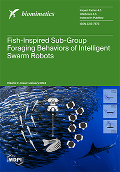
Fish exhibit an innate capacity to effectively sense and respond to their dynamic environments, often through very simple mechanisms and with limited available information. Fish schools demonstrate collective behaviors that enable them to cooperatively accomplish tasks that surpass the abilities of a single individual. This study develops a novel approach to swarm robotic systems, inspired by the foraging behavior of fish schools, which integrates a bio-inspired neural network and a self-organizing map algorithm, enabling swarm robots to exhibit fish-like behaviors such as collision-free navigation and dynamic sub-group formation. This research represents a unique integration of neurodynamic models and swarm intelligence to enhance the autonomous capabilities of individual robots and the collective efficiency of the swarm. View this paper
  • Issues are regarded as officially published after their release is announced to the table of contents alert mailing list.
  • You may sign up for e-mail alerts to receive table of contents of newly released issues.
  • PDF is the official format for papers published in both, html and pdf forms. To view the papers in pdf format, click on the "PDF Full-text" link, and use the free Adobe Reader to open them.
Order results
Result details
Section
Select all
Export citation of selected articles as:
14 pages, 5153 KiB  
Article
A Semi-Autonomous Hierarchical Control Framework for Prosthetic Hands Inspired by Dual Streams of Human
by Xuanyi Zhou, Jianhua Zhang, Bangchu Yang, Xiaolong Ma, Hao Fu, Shibo Cai and Guanjun Bao
Biomimetics 2024, 9(1), 62; https://doi.org/10.3390/biomimetics9010062 - 22 Jan 2024
Cited by 1 | Viewed by 1642
Abstract
The routine use of prosthetic hands significantly enhances amputees’ daily lives, yet it often introduces cognitive load and reduces reaction speed. To address this issue, we introduce a wearable semi-autonomous hierarchical control framework tailored for amputees. Drawing inspiration from the visual processing stream [...] Read more.
The routine use of prosthetic hands significantly enhances amputees’ daily lives, yet it often introduces cognitive load and reduces reaction speed. To address this issue, we introduce a wearable semi-autonomous hierarchical control framework tailored for amputees. Drawing inspiration from the visual processing stream in humans, a fully autonomous bionic controller is integrated into the prosthetic hand control system to offload cognitive burden, complemented by a Human-in-the-Loop (HIL) control method. In the ventral-stream phase, the controller integrates multi-modal information from the user’s hand–eye coordination and biological instincts to analyze the user’s movement intention and manipulate primitive switches in the variable domain of view. Transitioning to the dorsal-stream phase, precise force control is attained through the HIL control strategy, combining feedback from the prosthetic hand’s sensors and the user’s electromyographic (EMG) signals. The effectiveness of the proposed interface is demonstrated by the experimental results. Our approach presents a more effective method of interaction between a robotic control system and the human. Full article
(This article belongs to the Special Issue Bionic Technology—Robotic Exoskeletons and Prostheses: 2nd Edition)
Show Figures

Figure 1

Figure 1
<p>The framework of two nerve streams of visual information.</p>
Full article ">Figure 2
<p>Manipulate sequence planning for the controller.</p>
Full article ">Figure 3
<p>The myoelectric signal. (<b>a</b>) Original EMG signal. (<b>b</b>) Bandpass filtering.</p>
Full article ">Figure 4
<p>The procedures of the proportional control mode.</p>
Full article ">Figure 5
<p>Block diagram for grasping force control of prosthetic hand with the human in the control loop.</p>
Full article ">Figure 6
<p>Experimental setup.</p>
Full article ">Figure 7
<p>The view field from the subject’s perspective.</p>
Full article ">Figure 8
<p>Arm and hand collaborative control experiment.</p>
Full article ">Figure 9
<p>The cooperative manipulation experiment of a prosthetic hand and human hand.</p>
Full article ">Figure 10
<p>Framework of the semi-automatic controller for the prostheses hand.</p>
Full article ">
13 pages, 5389 KiB  
Review
Customized Subperiosteal Implants for the Rehabilitation of Atrophic Jaws: A Consensus Report and Literature Review
by Javier Herce-López, Mariano del Canto Pingarrón, Álvaro Tofé-Povedano, Laura García-Arana, Marc Espino-Segura-Illa, Ramón Sieira-Gil, Carlos Rodado-Alonso, Alba Sánchez-Torres and Rui Figueiredo
Biomimetics 2024, 9(1), 61; https://doi.org/10.3390/biomimetics9010061 - 22 Jan 2024
Cited by 5 | Viewed by 4160
Abstract
(1) Background: The aim was to perform a literature review on customized subperiosteal implants (CSIs) and provide clinical guidelines based on the results of an expert consensus meeting held in 2023. (2) Methods: A literature search was performed in Pubmed (MEDLINE) in July [...] Read more.
(1) Background: The aim was to perform a literature review on customized subperiosteal implants (CSIs) and provide clinical guidelines based on the results of an expert consensus meeting held in 2023. (2) Methods: A literature search was performed in Pubmed (MEDLINE) in July 2023, including case series and cohort studies with a minimum follow-up of 6 months that analyzed totally or partially edentulous patients treated with CSIs. Previously, an expert consensus meeting had been held in May 2023 to establish the most relevant clinical guidelines. (3) Results: Six papers (four case series and two retrospective cohort studies) were finally included in the review. Biological and mechanical complication rates ranged from 5.7% to 43.8% and from 6.3% to 20%, respectively. Thorough digital planning to ensure the passive fit of the CSI is mandatory to avoid implant failure. (4) Conclusions: CSIs are a promising treatment option for rehabilitating edentulous patients with atrophic jaws; they seem to have an excellent short-term survival rate, a low incidence of major complications, and less morbidity in comparison with complex bone grafting procedures. As the available data on the use of CSIs are very scarce, it is not possible to establish clinical recommendations based on scientific evidence. Full article
(This article belongs to the Special Issue Dentistry and Cranio Facial District: The Role of Biomimetics)
Show Figures

Figure 1

Figure 1
<p>Example of a suitably designed customized subperiosteal implant (CSI) with smooth transitions (without sharp angles) between the frame and the prosthetic connections.</p>
Full article ">Figure 2
<p>Example of a two-piece customized subperiosteal implant (CSI) designed for the patient’s specific anatomy. (<b>a</b>) Digital planning. (<b>b</b>) CSI placement.</p>
Full article ">Figure 3
<p>Surgical template used to remove the residual alveolar ridge. (<b>a</b>) Polyamide template. (<b>b</b>) Titanium alloy template. (<b>c</b>,<b>d</b>) CSI placement.</p>
Full article ">Figure 4
<p>Clinical images of soft tissue dehiscences. These are some of the most common complications associated with customized subperiosteal implants (CSI) but do not seem to affect the short-term success rate of the treatment. (<b>a</b>) Exposure of a maxillary CSI caused by a soft tissue dehiscence. (<b>b</b>) Soft tissue dehiscence and peri-implant mucosa inflammation in a maxillary CSI probably related to the abrupt transition between the frame and the prosthetic connection (see arrows).</p>
Full article ">Figure 5
<p>3D model of the patient with a customized subperiosteal implant (CSI).</p>
Full article ">
17 pages, 21110 KiB  
Article
Biomimetic Study of a Honeycomb Energy Absorption Structure Based on Straw Micro-Porous Structure
by Shucai Xu, Nuo Chen, Haoyi Qin, Meng Zou and Jiafeng Song
Biomimetics 2024, 9(1), 60; https://doi.org/10.3390/biomimetics9010060 - 21 Jan 2024
Viewed by 1862
Abstract
In this paper, sorghum and reed, which possess light stem structures in nature, were selected as biomimetic prototypes. Based on their mechanical stability characteristics—the porous structure at the node feature and the porous feature in the outer skin— biomimetic optimization design, simulation, and [...] Read more.
In this paper, sorghum and reed, which possess light stem structures in nature, were selected as biomimetic prototypes. Based on their mechanical stability characteristics—the porous structure at the node feature and the porous feature in the outer skin— biomimetic optimization design, simulation, and experimental research on both the traditional hexagonal structure and a hexagonal honeycomb structure were carried out. According to the two types of straw microcell and chamber structure characteristics, as well as the cellular energy absorption structure for the bionic optimization design, 22 honeycomb structures in 6 categories were considered, including a corrugated cell wall bionic design, a modular cell design, a reinforcement plate structure, and a self-similar structure, as well as a porous cell wall structure and gradient structures of variable wall thickness. Among them, HTPC-3 (a combined honeycomb structure), HSHT (a self-similar honeycomb structure), and HBCT-257 (a radial gradient variable wall thickness honeycomb structure) had the best performance: their energy absorption was 41.06%, 17.84%, and 83.59% higher than that of HHT (the traditional hexagonal honeycomb decoupling unit), respectively. Compared with HHT (a traditional hexagon honeycomb decoupling unit), the specific energy absorption was increased by 39.98%, 17.24%, and 26.61%, respectively. Verification test analysis revealed that the combined honeycomb structure performed the best and that its specific energy absorption was 22.82% higher than that of the traditional hexagonal structure. Full article
(This article belongs to the Special Issue Computer-Aided Biomimetics)
Show Figures

Figure 1

Figure 1
<p>Bionic prototype: (<b>a</b>) sorghum straw; and (<b>b</b>) reed straw.</p>
Full article ">Figure 2
<p>Characteristics of the microcellular structure of straw (SEM view): (<b>a</b>). crystal cell boundary line structure of longitudinal cross-section at reed node; (<b>b</b>). microstructure of vascular bundle at reed node; (<b>c</b>). microstructure of the outer sheath wall of <span class="html-italic">Phragmites australis</span>; (<b>d</b>). microstructure of large vascular bundle structure of sorghum; and (<b>e</b>). microstructure of small vascular bundle of sorghum straw (R1 is the inner circle radius of the large vascular bundle, and R2 is the outer circle radius of the small vascular bundle).</p>
Full article ">Figure 3
<p>Bionic design of honeycomb structures: (<b>a</b>). HTBC; (<b>b</b>). HHTBC-7; (<b>c</b>). HHTBC; (<b>d</b>). STBC; (<b>e</b>). HTPC-1; (<b>f</b>). HTPC-2; (<b>g</b>). HTPC-3; (<b>h</b>). OHT; (<b>i</b>). OHTBR; (<b>j</b>). HST; (<b>k</b>). HSHT; (<b>l</b>). CT; (<b>m</b>). CTBH; (<b>n</b>). CHT; (<b>o</b>). CHTBH; (<b>p</b>). HBVT-257; (<b>q</b>). HUT/HBVT-555; and (<b>r</b>) HBVT-752.</p>
Full article ">Figure 4
<p>Finite element simulation analysis model (example: radial-gradient variable-wall thickness honeycomb structure). This figure uses HBVT as an example to demonstrate its finite element simulation environment, where different grid colors from the inside out represent different wall thicknesses.</p>
Full article ">Figure 5
<p>Stress–strain curve of AA6061-T6.</p>
Full article ">Figure 6
<p>Force–displacement curves of each energy-absorbing structure under axial impact. (<b>a</b>). Load–displacement curves of the HT, HTBC, HHT-7, HHTBC-7, HHT, HHTBC, ST, and STBC. (<b>b</b>). Load–displacement curves of the HTPC-1, HTPC-2, HTPC-3, and HHT. (<b>c</b>) Load–displacement curves of the OHT, OHTBR, and HHT. (<b>d</b>). Load–displacement curves of the HT, HHT, HST, and HSHT. (<b>e</b>). Load–displacement curves of the CT, CTBH, CHT, and CHTBH. (<b>f</b>). Load–displacement curves of the HBVT-257, HUT/HBVT-555, and HBVT-752.</p>
Full article ">Figure 7
<p>Axial compression deformation and stress cloud in honeycomb structures: (<b>a</b>). HT; (<b>b</b>). HTBC; (<b>c</b>). HHT-7; (<b>d</b>). HHTBC-7; (<b>e</b>). HHT; (<b>f</b>). HHTBC; (<b>g</b>). ST; (<b>h</b>). STBC; (<b>i</b>). HTPC-1; (<b>j</b>). HTPC-2; (<b>k</b>). HTPC-3; (<b>l</b>). OHT; (<b>m</b>). OHTBR; (<b>n</b>). HST; (<b>o</b>). HSHT; (<b>p</b>). CT; (<b>q</b>). CTBH; (<b>r</b>). CHT; (<b>s</b>). CHTBH; (<b>t</b>). HBVT-257; (<b>u</b>). HUT/HBVT-555; and (<b>v</b>) HBVT-752.</p>
Full article ">Figure 7 Cont.
<p>Axial compression deformation and stress cloud in honeycomb structures: (<b>a</b>). HT; (<b>b</b>). HTBC; (<b>c</b>). HHT-7; (<b>d</b>). HHTBC-7; (<b>e</b>). HHT; (<b>f</b>). HHTBC; (<b>g</b>). ST; (<b>h</b>). STBC; (<b>i</b>). HTPC-1; (<b>j</b>). HTPC-2; (<b>k</b>). HTPC-3; (<b>l</b>). OHT; (<b>m</b>). OHTBR; (<b>n</b>). HST; (<b>o</b>). HSHT; (<b>p</b>). CT; (<b>q</b>). CTBH; (<b>r</b>). CHT; (<b>s</b>). CHTBH; (<b>t</b>). HBVT-257; (<b>u</b>). HUT/HBVT-555; and (<b>v</b>) HBVT-752.</p>
Full article ">Figure 8
<p>The energy absorption index of each structure under axial impact: (<b>a</b>). SEA and EA; and (<b>b</b>). PF and CFE.</p>
Full article ">Figure 9
<p>Three-dimensionally printed honeycomb structures: (<b>a</b>). HBVT-555; (<b>b</b>). HTPC-3; (<b>c</b>). OHT; (<b>d</b>). OHTBR; (<b>e</b>). HSHT; and (<b>f</b>). HBVT-257.</p>
Full article ">Figure 10
<p>Part of the 3D-printed honeycomb structure deformation process.</p>
Full article ">
18 pages, 3400 KiB  
Article
Design Optimization of a Hybrid-Driven Soft Surgical Robot with Biomimetic Constraints
by Majid Roshanfar, Javad Dargahi and Amir Hooshiar
Biomimetics 2024, 9(1), 59; https://doi.org/10.3390/biomimetics9010059 - 21 Jan 2024
Cited by 1 | Viewed by 2009
Abstract
The current study investigated the geometry optimization of a hybrid-driven (based on the combination of air pressure and tendon tension) soft robot for use in robot-assisted intra-bronchial intervention. Soft robots, made from compliant materials, have gained popularity for use in surgical interventions due [...] Read more.
The current study investigated the geometry optimization of a hybrid-driven (based on the combination of air pressure and tendon tension) soft robot for use in robot-assisted intra-bronchial intervention. Soft robots, made from compliant materials, have gained popularity for use in surgical interventions due to their dexterity and safety. The current study aimed to design a catheter-like soft robot with an improved performance by minimizing radial expansion during inflation and increasing the force exerted on targeted tissues through geometry optimization. To do so, a finite element analysis (FEA) was employed to optimize the soft robot’s geometry, considering a multi-objective goal function that incorporated factors such as chamber pressures, tendon tensions, and the cross-sectional area. To accomplish this, a cylindrical soft robot with three air chambers, three tendons, and a central working channel was considered. Then, the dimensions of the soft robot, including the length of the air chambers, the diameter of the air chambers, and the offsets of the air chambers and tendon routes, were optimized to minimize the goal function in an in-plane bending scenario. To accurately simulate the behavior of the soft robot, Ecoflex 00-50 samples were tested based on ISO 7743, and a hyperplastic model was fitted on the compression test data. The FEA simulations were performed using the response surface optimization (RSO) module in ANSYS software, which iteratively explored the design space based on defined objectives and constraints. Using RSO, 45 points of experiments were generated based on the geometrical and loading constraints. During the simulations, tendon force was applied to the tip of the soft robot, while simultaneously, air pressure was applied inside the chamber. Following the optimization of the geometry, a prototype of the soft robot with the optimized values was fabricated and tested in a phantom model, mimicking simulated surgical conditions. The decreased actuation effort and radial expansion of the soft robot resulting from the optimization process have the potential to increase the performance of the manipulator. This advancement led to improved control over the soft robot while additionally minimizing unnecessary cross-sectional expansion. The study demonstrates the effectiveness of the optimization methodology for refining the soft robot’s design and highlights its potential for enhancing surgical interventions. Full article
(This article belongs to the Special Issue Bio-Optimization-Based Soft Robot Design)
Show Figures

Figure 1

Figure 1
<p>Hybrid-driven soft surgical robot inside the lungs during an intra-bronchial intervention.</p>
Full article ">Figure 2
<p>Setup architecture of the hybrid air–tendon-driven soft robot for use in RAMIS.</p>
Full article ">Figure 3
<p>Design variables (<b>a</b>) <math display="inline"> <semantics> <msub> <mi>D</mi> <mi>w</mi> </msub> </semantics> </math> represents the diameter of the working channel, <math display="inline"> <semantics> <msub> <mi>D</mi> <mrow> <mi>c</mi> <mi>h</mi> </mrow> </msub> </semantics> </math> is the diameter of the air chambers, <math display="inline"> <semantics> <msub> <mi>D</mi> <mi>t</mi> </msub> </semantics> </math> is the diameter of the tendon passes, <math display="inline"> <semantics> <msub> <mi>D</mi> <mi>o</mi> </msub> </semantics> </math> is the outer diameter of the soft robot, and <math display="inline"> <semantics> <msub> <mi>a</mi> <mrow> <mi>c</mi> <mi>h</mi> </mrow> </msub> </semantics> </math> and <math display="inline"> <semantics> <msub> <mi>a</mi> <mi>t</mi> </msub> </semantics> </math> represent the offsets of the air chambers and tendon passes from the center of the cross-section, respectively. (<b>b</b>) <math display="inline"> <semantics> <msub> <mi>L</mi> <mrow> <mi>c</mi> <mi>h</mi> </mrow> </msub> </semantics> </math> represents the length of the air chambers.</p>
Full article ">Figure 4
<p>Compression test performed with Bose UTM on the Ecoflex-50 samples based on ISO 7743.</p>
Full article ">Figure 5
<p>(<b>a</b>) Engineering stress–strain compression curve (<b>b</b>) comprehensive compression–tension engineering stress–strain curve for Ecoflex 00-50. The tension data extracted from [<a href="#B61-biomimetics-09-00059" class="html-bibr">61</a>].</p>
Full article ">Figure 5 Cont.
<p>(<b>a</b>) Engineering stress–strain compression curve (<b>b</b>) comprehensive compression–tension engineering stress–strain curve for Ecoflex 00-50. The tension data extracted from [<a href="#B61-biomimetics-09-00059" class="html-bibr">61</a>].</p>
Full article ">Figure 6
<p>Deformation of the soft robot (<b>a</b>) caused by increasing the air pressure inside the air chamber and tendon tension (<b>b</b>) Cross-section of the soft robot, illustrating the chamber undergoing pressurization and the tendon being pulled.</p>
Full article ">Figure 7
<p>Variation in the bending angle of the soft robot vs. (<b>a</b>) the air chamber diameter, <math display="inline"> <semantics> <msub> <mi>D</mi> <mrow> <mi>C</mi> <mi>h</mi> </mrow> </msub> </semantics> </math>, (<b>b</b>) tendon offset <math display="inline"> <semantics> <msub> <mi>a</mi> <mi>t</mi> </msub> </semantics> </math>, (<b>c</b>) air chamber length <math display="inline"> <semantics> <msub> <mi>L</mi> <mrow> <mi>C</mi> <mi>h</mi> </mrow> </msub> </semantics> </math>, and- (<b>d</b>) air chamber offset <math display="inline"> <semantics> <msub> <mi>a</mi> <mrow> <mi>C</mi> <mi>h</mi> </mrow> </msub> </semantics> </math>.</p>
Full article ">Figure 8
<p>Deformation of the soft robot with the optimized parameters (<b>a</b>) variation in the bending angle vs. the air chamber diameter and offset. (<b>b</b>) Variation in the bending angle vs. the tendon force and air chamber pressure. (<b>c</b>) Variation in the outer radius of the soft robot vs. the air chamber pressure and diameter.</p>
Full article ">Figure 9
<p>Mold design of the hybrid air–tendon-driven soft robot with a central working channel.</p>
Full article ">Figure 10
<p>Linear actuator of the soft robot: ① NEMA 17 stepper motor, ② shaft coupler, ③ EPOS4 3-axes digital positioning controller of the motors, ④ silicone tube, ⑤ holder of the robotic arm, ⑥ double bearing and lead screw, ⑦ bearing, ⑧ screws, and ⑨ brushless DC motor with Hall sensors.</p>
Full article ">Figure 11
<p>Integrated hybrid-driven soft robot into the CRS robotic arm and the phantom model.</p>
Full article ">
22 pages, 4056 KiB  
Article
Perceived Safety Assessment of Interactive Motions in Human–Soft Robot Interaction
by Yun Wang, Gang Wang, Weihan Ge, Jinxi Duan, Zixin Chen and Li Wen
Biomimetics 2024, 9(1), 58; https://doi.org/10.3390/biomimetics9010058 - 21 Jan 2024
Cited by 1 | Viewed by 1746
Abstract
Soft robots, especially soft robotic hands, possess prominent potential for applications in close proximity and direct contact interaction with humans due to their softness and compliant nature. The safety perception of users during interactions with soft robots plays a crucial role in influencing [...] Read more.
Soft robots, especially soft robotic hands, possess prominent potential for applications in close proximity and direct contact interaction with humans due to their softness and compliant nature. The safety perception of users during interactions with soft robots plays a crucial role in influencing trust, adaptability, and overall interaction outcomes in human–robot interaction (HRI). Although soft robots have been claimed to be safe for over a decade, research addressing the perceived safety of soft robots still needs to be undertaken. The current safety guidelines for rigid robots in HRI are unsuitable for soft robots. In this paper, we highlight the distinctive safety issues associated with soft robots and propose a framework for evaluating the perceived safety in human–soft robot interaction (HSRI). User experiments were conducted, employing a combination of quantitative and qualitative methods, to assess the perceived safety of 15 interactive motions executed by a soft humanoid robotic hand. We analyzed the characteristics of safe interactive motions, the primary factors influencing user safety assessments, and the impact of motion semantic clarity, user technical acceptance, and risk tolerance level on safety perception. Based on the analyzed characteristics, we summarize vital insights to provide valuable guidelines for designing safe, interactive motions in HSRI. The current results may pave the way for developing future soft machines that can safely interact with humans and their surroundings. Full article
(This article belongs to the Special Issue Bio-Inspired Technologies and Soft Robotics)
Show Figures

Figure 1

Figure 1
<p>(<b>a</b>,<b>b</b>) Soft robotic gripper [<a href="#B29-biomimetics-09-00058" class="html-bibr">29</a>,<a href="#B31-biomimetics-09-00058" class="html-bibr">31</a>]; (<b>c</b>) soft neuro-prosthetic hand [<a href="#B28-biomimetics-09-00058" class="html-bibr">28</a>]; (<b>d</b>) human teaching soft robot to perform tasks [<a href="#B32-biomimetics-09-00058" class="html-bibr">32</a>]; (<b>e</b>) soft robot for hand rehabilitation [<a href="#B33-biomimetics-09-00058" class="html-bibr">33</a>]; (<b>f</b>) soft robotic hand with human-inspired soft palm [<a href="#B34-biomimetics-09-00058" class="html-bibr">34</a>]. Reprinted with permission from Ref. [<a href="#B28-biomimetics-09-00058" class="html-bibr">28</a>]. 2023, Guoying Gu et al.; Reprinted with permission from Ref. [<a href="#B31-biomimetics-09-00058" class="html-bibr">31</a>]. 2023, Wenbo Liu et al.; Adapted with permission from Ref. [<a href="#B32-biomimetics-09-00058" class="html-bibr">32</a>]. 2022, Wenbo Liu et al.; Reprinted with permission from Ref. [<a href="#B33-biomimetics-09-00058" class="html-bibr">33</a>]. 2022, Zhi Qiang Tang; Reprinted with permission from Ref. [<a href="#B34-biomimetics-09-00058" class="html-bibr">34</a>]. open access.</p>
Full article ">Figure 2
<p>Evaluation frameworks [<a href="#B39-biomimetics-09-00058" class="html-bibr">39</a>,<a href="#B46-biomimetics-09-00058" class="html-bibr">46</a>,<a href="#B50-biomimetics-09-00058" class="html-bibr">50</a>].</p>
Full article ">Figure 3
<p>(<b>a</b>) Fabrication process of the soft robotic hands; (<b>b</b>) final result.</p>
Full article ">Figure 4
<p>(<b>a</b>) Recorded interactive motions; (<b>b</b>) different stage of user experiment.</p>
Full article ">Figure 5
<p>(<b>a</b>) Ranking of evaluation factors based on self-report of participants from different groups; (<b>b</b>) perceived safety score and semantic clarity of all the 15 interactive motions.</p>
Full article ">Figure 6
<p>(<b>a</b>) Different perceived safety scores between the four different participant types, compared to average scores; (<b>b</b>) trends in level of relaxation between participants with different levels of soft robot acceptance and risk toleration.</p>
Full article ">Figure 7
<p>Gaze heatmaps in different motion stages of (<b>a</b>) grasping, (<b>b</b>) sudden release, and (<b>c</b>) slow stroking.</p>
Full article ">
13 pages, 2499 KiB  
Article
One-Step Purification of Recombinant Cutinase from an E. coli Extract Using a Stabilizing Triazine-Scaffolded Synthetic Affinity Ligand
by Luís P. Fonseca and M. Ângela Taipa
Biomimetics 2024, 9(1), 57; https://doi.org/10.3390/biomimetics9010057 - 20 Jan 2024
Viewed by 1484
Abstract
Cutinase from Fusarium solani pisi is an enzyme that bridges functional properties between lipases and esterases, with applications in detergents, food processing, and the synthesis of fine chemicals. The purification procedure of recombinant cutinase from E. coil extracts is a well-established but time-consuming [...] Read more.
Cutinase from Fusarium solani pisi is an enzyme that bridges functional properties between lipases and esterases, with applications in detergents, food processing, and the synthesis of fine chemicals. The purification procedure of recombinant cutinase from E. coil extracts is a well-established but time-consuming process, which involves a sequence of two anionic exchange chromatography steps followed by dialysis. Affinity chromatography is the most efficient method for protein purification, the major limitation of its use being often the availability of a ligand selective for a given target protein. Synthetic affinity ligands that specifically recognize certain sites on the surface of proteins are highly desirable for affinity processes due to their cost-effectiveness, durability, and reusability across multiple cycles. Additionally, these ligands establish moderate affinity interactions with the target protein, making it possible to purify proteins under gentle conditions while maintaining high levels of activity recovery. This study aimed to develop a new method for purifying cutinase, utilizing triazine-scaffolded biomimetic affinity ligands. These ligands were previously screened from a biased-combinatorial library to ensure their binding ability to cutinase without compromising its biological function. A lead ligand, designated as 11/3′, [4-({4-chloro-6-[(2-methylbutyl)amino]-1,3,5-triazin-2-yl}amino)benzoic acid], was chosen and directly synthesized onto agarose. Experiments conducted at different scales demonstrated that this ligand (with an affinity constant Ka ≈ 104 M−1) exhibited selectivity towards cutinase, enabling the purification of the enzyme from an E. coli crude production medium in a single step. Under optimized conditions, the protein and activity yields reached 25% and 90%, respectively, with a resulting cutinase purity of 85%. Full article
(This article belongs to the Special Issue Biomimetic Peptides and Proteins)
Show Figures

Graphical abstract

Graphical abstract
Full article ">Figure 1
<p>Screening of synthetic affinity ligands from a combinatorial library for cutinase purification by affinity chromatography. Recovered protein yields in the elution step (grey), activity yields at the elution step (black), and cutinase purity degree (no fill) at the main elution peak are represented for the affinity chromatographic assays performed with all the solid-phase screened ligands.</p>
Full article ">Figure 2
<p>Silver-stained SDS-PAGE gels of the control (<b>left</b>) and scale-up (<b>right</b>) experiments, using the <span class="html-italic">de novo</span> synthetized solid-phase ligand 11/3′ for cutinase purification by affinity chromatography. Each well was loaded with 1 µg of total protein. On the left: lane 1, molecular weight marker; lane 2, breakthrough; lane 3, washing pool; lane 4, total elution pool (elution peak + elution pool). On the right: lane 1, molecular weight marker; lane 2, breakthrough; lane 3, washing pool; lane 4, elution peak; lane 5, elution pool. Arrows indicate the position of the protein band corresponding to cutinase.</p>
Full article ">Figure 3
<p>Chromatogram of the scale-up assay, using newly synthetized ligand 11/3′ for cutinase purification by affinity chromatography. Absorbance at 280 nm was measured for protein quantification (blue line). The elution peak is highlighted on the right, denoting a dragged protein elution after the elution peak. The fractions collected during elution are represented in red in the highlighted section. The waste corresponds to column regeneration with 0.1 M NaOH, 30% (<span class="html-italic">v</span>/<span class="html-italic">v</span>) isopropanol.</p>
Full article ">Figure 4
<p>Assessment of different elution buffers for improvement of cutinase elution and purification. Protein yields (grey), activity yields (black), and purification factors (dotted) obtained at the <span class="underline">main elution peak</span> with the different elution buffers tested for cutinase purification by affinity chromatography with the <span class="html-italic">de novo</span> synthetized ligand 11/3′. The control corresponds to elution buffer 1.</p>
Full article ">Figure 5
<p>SDS-PAGE analysis of the effect of elution buffers 4 and 5 on cutinase purification, with the <span class="html-italic">de novo</span> synthetized ligand 11/3′. Each well was loaded with 1 µg of total protein. Lanes 2–5 represent the affinity chromatographic process with elution buffer 4. Lanes 6–9 correspond to the process with elution buffer 5. Lane 1, molecular weight marker. Lane 2, breakthrough. Lane 3, washing pool. Lane 4, elution peak. Lane 5, elution pool. Lane 6, breakthrough. Lane 7, washing pool. Lane 8, elution peak. Lane 9, elution pool. Lane 10, first dialysis extract. Arrows indicate the position of the protein band corresponding to cutinase.</p>
Full article ">
22 pages, 6665 KiB  
Article
Design and Reality-Based Modeling Optimization of a Flexible Passive Joint Paddle for Swimming Robots
by Junzhe Hu, Yaohui Xu, Pengyu Chen, Fengran Xie, Hanlin Li and Kai He
Biomimetics 2024, 9(1), 56; https://doi.org/10.3390/biomimetics9010056 - 19 Jan 2024
Viewed by 1594
Abstract
Rowing motion with paired propellers is an essential actuation mechanism for swimming robots. Previous work in this field has typically employed flexible propellers to generate a net thrust or torque by using changes in the compliance values of flexible structures under the influence [...] Read more.
Rowing motion with paired propellers is an essential actuation mechanism for swimming robots. Previous work in this field has typically employed flexible propellers to generate a net thrust or torque by using changes in the compliance values of flexible structures under the influence of a fluid. The low stiffness values of the flexible structures restrict the upper limit of the oscillation frequency and amplitude, resulting in slow swimming speeds. Furthermore, complex coupling between the fluid and the propeller reduce the accuracy of flexible propeller simulations. A design of a flexible passive joint paddle was proposed in this study, and a dynamics model and simulation of the paddle were experimentally verified. In order to optimize the straight swimming speed, a data-driven model was proposed to improve the simulation accuracy. The effects of the joint number and controller parameters on the robot’s straight swimming speed were comprehensively investigated. The multi-joint paddle exhibited significantly improved thrust over the single-joint paddle in a symmetric driving mode. The data-driven model reduced the total error of the simulated data of the propulsive force in the range of control parameters to 0.51%. Swimming speed increased by 3.3 times compared to baseline. These findings demonstrate the utility of the proposed dynamics and data-driven models in the multi-objective design of swimming robots. Full article
(This article belongs to the Special Issue Bio-Inspired Underwater Robot)
Show Figures

Figure 1

Figure 1
<p>The bionic design of swimming robot. (<b>a</b>) The diving beetle and the structure of its flexible swimming legs. (<b>b</b>) The swimming robot and flexible passive joint paddle inspired by diving beetles.</p>
Full article ">Figure 2
<p>Schematic diagram of flexible passive joint paddles (FPJP) design. (<b>a</b>) Principle of the FPJP with three flexible joints (FP3JP, abbreviations for FPJPs with one and two flexible joints are defined similarly). (<b>b</b>) Morphological changes of the FPJP during the power stroke and recovery stroke on swimming robot platform.</p>
Full article ">Figure 3
<p>Dynamics model of the flexible passive joint paddle (FPJP). (<b>a</b>) Top view schematic of the FPJP in the recovery stroke. (<b>b</b>) Top view schematic of the FPJP in the power stroke.</p>
Full article ">Figure 4
<p>Validation of the simulation model by high-speed camera. (<b>a</b>) The motion state of the FPJP was recorded and detected using a high-speed camera. The red arrow illustrates the rotation direction of the motion. FPJP motion characteristics with a paddle oscillation frequency of 0.6 Hz and amplitude of 75°: Variations of joint angle over one movement cycle for (<b>b</b>) FP1JP, (<b>c</b>) FP2JP, and (<b>d</b>) FP3JP; solid lines represent simulated data and dashed lines represent real data. (<b>e</b>) Changes in FP3JP morphology based on simulated data during a cycle.</p>
Full article ">Figure 5
<p>(<b>a</b>) Distribution of <math display="inline"> <semantics> <mrow> <mi>C</mi> <mi>n</mi> </mrow> </semantics> </math>. (<b>b</b>–<b>f</b>) Pre-transform simulation, experimental, post-transformation (<math display="inline"> <semantics> <mrow> <mi>C</mi> <mi>n</mi> </mrow> </semantics> </math>, SVD, and Cn-SVD) average thrust thermograms for varying oscillation amplitude <span class="html-italic">A</span> and frequency <span class="html-italic">f</span>, demonstrating the successful error reduction between the experiment and simulated data. The symbol in each figure shows the oscillation amplitude and frequency generating the largest average force.</p>
Full article ">Figure 6
<p>Overall process and logic of the work.</p>
Full article ">Figure 7
<p>Comparison of the average error with the experimental data for real ratios of <math display="inline"> <semantics> <mrow> <mi mathvariant="normal">r</mi> <mo>∈</mo> <mo>[</mo> <mn>0</mn> <mo>,</mo> <mn>0.25</mn><mo>]</mo> </mrow> </semantics> </math>: simulated data, simulated data with <math display="inline"> <semantics> <mrow> <mi>C</mi> <mi>n</mi> </mrow> </semantics> </math>, simulated data after SVD transformation, and simulated data of the novel Cn-SVD combined data-driven model.</p>
Full article ">Figure 8
<p>Experimental setup. (<b>a</b>) High-speed camera with a force measurement system. (<b>b</b>) Schematic diagram of the composition of the force measurement system. (<b>c</b>) User interface and PXI system. (<b>d</b>) Design specifications of the diving-beetle-like swimming robot (DBSR). (<b>e</b>) Hardware configuration inside the DBSR body. (<b>f</b>) Swimming behavior of the DBSR observed from the top view.</p>
Full article ">Figure 9
<p>(<b>a</b>) Representative time series from FP1JP, FP2JP, and FP3JP thrust tests. (<b>b</b>) Average thrust of the two-joint paddle with multiple control parameters (amplitude and frequency). (<b>c</b>) Distributions of the differences between the average thrust values of the two-joint paddle and those of the three-joint (red) and one-joint (blue) paddles.</p>
Full article ">Figure 10
<p>(<b>a</b>) Experiment of DBSR while swimming. The red dashed line is the reference line. (<b>b</b>) Comparison of robot velocities with FP1JP and FP3JP for different frequencies and amplitudes of 75° (solid lines) and 30° (dashed lines). (<b>c</b>) Yaw angle distribution of DBSR swimming straight with different control parameters.</p>
Full article ">
21 pages, 9987 KiB  
Article
In Vitro Studies on 3D-Printed PLA/HA/GNP Structures for Bone Tissue Regeneration
by Andreea-Mariana Negrescu, Aura-Cătălina Mocanu, Florin Miculescu, Valentina Mitran, Andreea-Elena Constantinescu and Anisoara Cimpean
Biomimetics 2024, 9(1), 55; https://doi.org/10.3390/biomimetics9010055 - 19 Jan 2024
Cited by 3 | Viewed by 2085
Abstract
The successful regeneration of large-size bone defects remains one of the most critical challenges faced in orthopaedics. Recently, 3D printing technology has been widely used to fabricate reliable, reproducible and economically affordable scaffolds with specifically designed shapes and porosity, capable of providing sufficient [...] Read more.
The successful regeneration of large-size bone defects remains one of the most critical challenges faced in orthopaedics. Recently, 3D printing technology has been widely used to fabricate reliable, reproducible and economically affordable scaffolds with specifically designed shapes and porosity, capable of providing sufficient biomimetic cues for a desired cellular behaviour. Natural or synthetic polymers reinforced with active bioceramics and/or graphene derivatives have demonstrated adequate mechanical properties and a proper cellular response, attracting the attention of researchers in the bone regeneration field. In the present work, 3D-printed graphene nanoplatelet (GNP)-reinforced polylactic acid (PLA)/hydroxyapatite (HA) composite scaffolds were fabricated using the fused deposition modelling (FDM) technique. The in vitro response of the MC3T3-E1 pre-osteoblasts and RAW 264.7 macrophages revealed that these newly designed scaffolds exhibited various survival rates and a sustained proliferation. Moreover, as expected, the addition of HA into the PLA matrix contributed to mimicking a bone extracellular matrix, leading to positive effects on the pre-osteoblast osteogenic differentiation. In addition, a limited inflammatory response was also observed. Overall, the results suggest the great potential of the newly developed 3D-printed composite materials as suitable candidates for bone tissue engineering applications. Full article
Show Figures

Figure 1

Figure 1
<p>Morphological evaluation on the outer surface of the 3D-printed products prepared with PLA/HA (0–30 wt.%)/GNP (0–3 wt.%). The yellow arrows are indicative of the boundaries of the printed lines. Scale bar: 1 mm.</p>
Full article ">Figure 2
<p>Viability of MC3T3-E1 cells grown in direct contact with the surface of the analysed samples after 24 h and 96 h of culture through the live and dead assay which allows the distinction between viable (green fluorescence) and dead (red fluorescence) cells. Scale bar represents 200 μm.</p>
Full article ">Figure 3
<p>CCK-8 assay highlighting the relative viability vs. the TCPS control sample of the MC3T3-E1 pre-osteoblasts grown in direct contact with the analysed materials for 24 h and 96 h. Data analysis was based on mean ± SD, and the results are expressed as % of control (<span class="html-italic">n</span> = 3; **** <span class="html-italic">p</span> &lt; 0.0001 vs. TCPS; ●●●● <span class="html-italic">p</span> &lt; 0.0001, ●● <span class="html-italic">p</span> &lt; 0.01, ● <span class="html-italic">p</span> &lt; 0.05 vs. 0% GNP 0% HA; ○○○○ <span class="html-italic">p</span> &lt; 0.0001, ○ <span class="html-italic">p</span> &lt; 0.05 vs. 0% GNP 10% HA; ^^^^ <span class="html-italic">p</span> &lt; 0.0001,^^^ <span class="html-italic">p</span> &lt; 0.001, ^ <span class="html-italic">p</span> &lt; 0.05 vs. 0% GNP 20% HA; ■■■■ <span class="html-italic">p</span> &lt; 0.0001, ■■■ <span class="html-italic">p</span> &lt; 0.001, ■■ <span class="html-italic">p</span> &lt; 0.01 vs. 0% GNP 30% HA; #### <span class="html-italic">p</span> &lt; 0.0001, ### <span class="html-italic">p</span> &lt; 0.001, ## <span class="html-italic">p</span> &lt; 0.01, # <span class="html-italic">p</span> &lt; 0.05 vs. 1% GNP 0% HA; ++++ <span class="html-italic">p</span> &lt; 0.0001, + <span class="html-italic">p</span> &lt; 0.05 vs. 1% GNP 10% HA; ♦♦♦♦ <span class="html-italic">p</span> &lt; 0.0001, ♦♦♦ <span class="html-italic">p</span> &lt; 0.001 vs. 1% GNP 20% HA; ❖❖❖❖ <span class="html-italic">p</span> &lt; 0.0001 vs. 1% GNP 30% HA; □□□□ <span class="html-italic">p</span> &lt; 0.0001 vs. 2% GNP 0% HA; ⌘⌘⌘⌘ <span class="html-italic">p</span> &lt; 0.0001 vs. 2% GNP 10% HA; XXXX <span class="html-italic">p</span> &lt; 0.0001, XXX <span class="html-italic">p</span> &lt; 0.001, XX <span class="html-italic">p</span> &lt; 0.01 vs. 2% GNP 20% HA; ££££ <span class="html-italic">p</span> &lt; 0.0001, ££ <span class="html-italic">p</span> &lt; 0.01 vs. 2% GNP 30% HA;▽ <span class="html-italic">p</span> &lt; 0.05 vs. 3% GNP 0% HA; ▷ <span class="html-italic">p</span> &lt; 0.05 vs. 3% GNP 10% HA; <span class="html-fig-inline" id="biomimetics-09-00055-i001"><img alt="Biomimetics 09 00055 i001" src="/biomimetics/biomimetics-09-00055/article_deploy/html/images/biomimetics-09-00055-i001.png"/></span> <span class="html-italic">p</span> &lt; 0.05 vs. 3% GNP 20% HA).</p>
Full article ">Figure 4
<p>Representative fluorescence images of the morphological characteristics exhibited by the MC3T3-E1 cells grown onto the surface of the tested supports after 24 h and 96 h of culture (actin cytoskeleton—green fluorescence; nuclei—blue fluorescence). Scale bar represents 50 µm.</p>
Full article ">Figure 5
<p>Intracellular ALP activity exhibited by the MC3T3-E1 cells grown directly onto the surface of the analysed supports after 7 and 14 days of culture. Data analysis was based on mean ± SD (n = 3; **** <span class="html-italic">p</span> &lt; 0.0001, *** <span class="html-italic">p</span> &lt; 0.001, ** <span class="html-italic">p</span> &lt; 0.01, * <span class="html-italic">p</span> &lt; 0.05 vs. TCPS (-); <span class="html-italic">ffff p</span> &lt; 0.0001, <span class="html-italic">ff</span> &lt; 0.01 vs. TCPS (+); ●●●● <span class="html-italic">p</span> &lt; 0.0001, ●● <span class="html-italic">p</span> &lt; 0.01, ● <span class="html-italic">p</span> &lt; 0.05 vs. 0% GNP 0% HA; ○○○○ <span class="html-italic">p</span> &lt; 0.0001, ○○○ <span class="html-italic">p</span> &lt; 0.001, ○ <span class="html-italic">p</span> &lt; 0.05 vs. 0% GNP 10% HA; ^^^^ <span class="html-italic">p</span> &lt; 0.0001, ^^^ <span class="html-italic">p</span> &lt; 0.001, ^^ <span class="html-italic">p</span> &lt; 0.01, ^ <span class="html-italic">p</span> &lt; 0.05 vs. 0% GNP 20% HA; ■■■■ <span class="html-italic">p</span> &lt; 0.0001, ■■■ <span class="html-italic">p</span> &lt; 0.001, ■■ <span class="html-italic">p</span> &lt; 0.01, ■ <span class="html-italic">p</span> &lt; 0.05 vs. 0% GNP 30% HA; #### <span class="html-italic">p</span> &lt; 0.0001, ### <span class="html-italic">p</span> &lt; 0.001, ## <span class="html-italic">p</span> &lt; 0.01, # <span class="html-italic">p</span> &lt; 0.05 vs. 1% GNP 0% HA; ++++ <span class="html-italic">p</span> &lt; 0.0001, +++ <span class="html-italic">p</span> &lt; 0.001, + <span class="html-italic">p</span> &lt; 0.05 vs. 1% GNP 10% HA; ♦♦♦♦ <span class="html-italic">p</span> &lt; 0.0001, ♦♦♦ <span class="html-italic">p</span> &lt; 0.001, ♦♦ <span class="html-italic">p</span> &lt; 0.01, ♦ <span class="html-italic">p</span> &lt; 0.05 vs. 1% GNP 20% HA; ❖❖❖❖ <span class="html-italic">p</span> &lt; 0.0001, ❖❖❖ <span class="html-italic">p</span> &lt; 0.001, ❖❖ <span class="html-italic">p</span> &lt; 0.01,❖ <span class="html-italic">p</span> &lt; 0.05 vs. 1% GNP 30% HA; □□□□ <span class="html-italic">p</span> &lt; 0.0001, □□□ <span class="html-italic">p</span> &lt; 0.001, □□ <span class="html-italic">p</span> &lt; 0.01, □ <span class="html-italic">p</span> &lt; 0.05 vs. 2% GNP 0% HA; ⌘⌘⌘⌘ <span class="html-italic">p</span> &lt; 0.0001, ⌘⌘ <span class="html-italic">p</span> &lt; 0.01, ⌘ <span class="html-italic">p</span> &lt; 0.05 vs. 2% GNP 10% HA; XXXX <span class="html-italic">p</span> &lt; 0.0001, XXX <span class="html-italic">p</span> &lt; 0.001, XX <span class="html-italic">p</span> &lt; 0.01 vs. 2% GNP 20% HA; <span class="html-italic">££££ p</span> &lt; 0.0001 vs. 2% GNP 30% HA; ▽▽ <span class="html-italic">p</span> &lt; 0.01, ▽ <span class="html-italic">p</span> &lt; 0.05 vs. 3% GNP 0% HA; ▷▷ <span class="html-italic">p</span> &lt; 0.01, ▷ <span class="html-italic">p</span> &lt; 0.05 vs. 3% GNP 10% HA; <span class="html-fig-inline" id="biomimetics-09-00055-i002"><img alt="Biomimetics 09 00055 i002" src="/biomimetics/biomimetics-09-00055/article_deploy/html/images/biomimetics-09-00055-i002.png"/></span> <span class="html-italic">p</span> &lt; 0.001 vs. 3% GNP 20% HA). The TCPS (-) and TCPS (+) notations denote the negative and positive controls for pre-osteoblast differentiation, respectively.</p>
Full article ">Figure 6
<p>The quantitative analysis of (<b>a</b>) collagen synthesis and (<b>b</b>) calcium nodules deposition by MC3T3-E1 cells grown directly onto the surface of the analysed samples. Data analysis was based on mean ± SD (n = 3; **** <span class="html-italic">p</span> &lt; 0.0001, *** <span class="html-italic">p</span> &lt; 0.001, ** <span class="html-italic">p</span> &lt; 0.01, * <span class="html-italic">p</span> &lt; 0.05 vs. TCPS (-); <span class="html-italic">ffff p</span> &lt; 0.0001 vs. TCPS (+) ●●●● <span class="html-italic">p</span> &lt; 0.0001, ●●● <span class="html-italic">p</span> &lt; 0.001, ●● <span class="html-italic">p</span> &lt; 0.01, ● <span class="html-italic">p</span> &lt; 0.05 vs. 0% GNP 0% HA; ○○○○ <span class="html-italic">p</span> &lt; 0.0001, ○○○ <span class="html-italic">p</span> &lt; 0.001, ○○ <span class="html-italic">p</span> &lt; 0.01, ○ <span class="html-italic">p</span> &lt; 0.05 vs. 0% GNP 10% HA; ^^^^ <span class="html-italic">p</span> &lt; 0.0001, ^^^ <span class="html-italic">p</span> &lt; 0.001, ^^ <span class="html-italic">p</span> &lt; 0.01, ^ <span class="html-italic">p</span> &lt; 0.05 vs. 0% GNP 20% HA; ■■■■ <span class="html-italic">p</span> &lt; 0.0001, ■■■ <span class="html-italic">p</span> &lt; 0.001, ■■ <span class="html-italic">p</span> &lt; 0.01 vs. 0% GNP 30% HA; #### <span class="html-italic">p</span> &lt; 0.0001, ### <span class="html-italic">p</span> &lt; 0.001, ## <span class="html-italic">p</span> &lt; 0.01, # <span class="html-italic">p</span> &lt; 0.05 vs. 1% GNP 0% HA; ++++ <span class="html-italic">p</span> &lt; 0.0001, +++ <span class="html-italic">p</span> &lt; 0.001, ++ <span class="html-italic">p</span> &lt; 0.01, + <span class="html-italic">p</span> &lt; 0.05 vs. 1% GNP 10% HA; ♦♦♦♦ <span class="html-italic">p</span> &lt; 0.0001, ♦♦♦ <span class="html-italic">p</span> &lt; 0.001 vs. 1% GNP 20% HA; ❖❖❖❖ <span class="html-italic">p</span> &lt; 0.0001,❖❖❖ <span class="html-italic">p</span> &lt; 0.001 vs. 1% GNP 30% HA; □□□□ <span class="html-italic">p</span> &lt; 0.0001, □□□ <span class="html-italic">p</span> &lt; 0.001, □□ <span class="html-italic">p</span> &lt; 0.01, □ <span class="html-italic">p</span> &lt; 0.05 vs. 2% GNP 0% HA; ⌘⌘⌘⌘ <span class="html-italic">p</span> &lt; 0.0001, ⌘⌘ <span class="html-italic">p</span> &lt; 0.01, ⌘ <span class="html-italic">p</span> &lt; 0.05 vs. 2% GNP 10% HA; XXXX <span class="html-italic">p</span> &lt; 0.0001, XX <span class="html-italic">p</span> &lt; 0.01 vs. 2% GNP 20% HA; <span class="html-italic">££££ p</span> &lt; 0.0001, <span class="html-italic">££ p</span> &lt; 0.01 vs. 2% GNP 30% HA; ▽▽▽▽ <span class="html-italic">p</span> &lt; 0.0001, ▽▽▽ <span class="html-italic">p</span> &lt; 0.001 vs. 3% GNP 0% HA; ▷▷▷▷ <span class="html-italic">p</span> &lt; 0.0001, ▷▷ <span class="html-italic">p</span> &lt; 0.01 vs. 3% GNP 10% HA; <span class="html-fig-inline" id="biomimetics-09-00055-i003"><img alt="Biomimetics 09 00055 i003" src="/biomimetics/biomimetics-09-00055/article_deploy/html/images/biomimetics-09-00055-i003.png"/></span> <span class="html-italic">p</span> &lt; 0.001, <span class="html-fig-inline" id="biomimetics-09-00055-i004"><img alt="Biomimetics 09 00055 i004" src="/biomimetics/biomimetics-09-00055/article_deploy/html/images/biomimetics-09-00055-i004.png"/></span> <span class="html-italic">p</span> &lt; 0.01 vs. 3% GNP 20% HA). The TCPS (-) and TCPS (+) notations denote the negative and positive controls for pre-osteoblast differentiation, respectively.</p>
Full article ">Figure 7
<p>The relative viability vs. the TCPS (-) control sample of the RAW 264.7 macrophages grown in direct contact with the analysed materials, as assessed using the CCK-8 test at 24 h and 72 h post seeding (under proinflammatory stimulation with 100 ng/mL LPS, with the exception of the TCPS (-) sample). Data analysis was based on mean ± SD, and the results are expressed as % of the TCPS (-) control (n = 3, **** <span class="html-italic">p</span> &lt; 0.0001 vs. TCPS (-); <span class="html-italic">ffff p</span> &lt; 0.0001 vs. TCPS (+); ●●●● <span class="html-italic">p</span> &lt; 0.0001, ●●● <span class="html-italic">p</span> &lt; 0.001, ●● <span class="html-italic">p</span> &lt; 0.01 vs. 0% GNP 0% HA; ○○○○ <span class="html-italic">p</span> &lt; 0.0001, ○○○ <span class="html-italic">p</span> &lt; 0.001, ○○ <span class="html-italic">p</span> &lt; 0.01, ○ <span class="html-italic">p</span> &lt; 0.05 vs. 0% GNP 10% HA; ^^^^ <span class="html-italic">p</span> &lt; 0.0001, ^^^ <span class="html-italic">p</span> &lt; 0.001, ^^ <span class="html-italic">p</span> &lt; 0.01, ^ <span class="html-italic">p</span> &lt; 0.05 vs. 0% GNP 20% HA; ■■■■ <span class="html-italic">p</span> &lt; 0.0001, ■■ <span class="html-italic">p</span> &lt; 0.01, ■ <span class="html-italic">p</span> &lt; 0.05 vs. 0% GNP 30% HA; #### <span class="html-italic">p</span> &lt; 0.0001, ### <span class="html-italic">p</span> &lt; 0.001, ## <span class="html-italic">p</span> &lt; 0.01, # <span class="html-italic">p</span> &lt; 0.05 vs. 1% GNP 0% HA; ++++ <span class="html-italic">p</span> &lt; 0.0001, +++ <span class="html-italic">p</span> &lt; 0.001, ++ <span class="html-italic">p</span> &lt; 0.01 vs. 1% GNP 0% HA; ♦♦♦♦ <span class="html-italic">p</span> &lt; 0.0001, ♦♦♦ <span class="html-italic">p</span> &lt; 0.001, ♦ <span class="html-italic">p</span> &lt; 0.05 vs. 1% GNP 20% HA; ❖❖❖❖ <span class="html-italic">p</span> &lt; 0.0001, ❖❖ <span class="html-italic">p</span> &lt; 0.01 vs. 1% GNP 30% HA; □□□□ <span class="html-italic">p</span> &lt; 0.0001, □□□ <span class="html-italic">p</span> &lt; 0.001, □□ <span class="html-italic">p</span> &lt; 0.01 vs. 2% GNP 0% HA; ⌘⌘⌘⌘ <span class="html-italic">p</span> &lt; 0.0001, ⌘⌘ <span class="html-italic">p</span> &lt; 0.01, ⌘ <span class="html-italic">p</span> &lt; 0.05 vs. 2% GNP 10% HA; XXXX <span class="html-italic">p</span> &lt; 0.0001, XX &lt; 0.01 vs 2% GNP 20 % HA; ££££ <span class="html-italic">p</span> &lt; 0.0001, ££ <span class="html-italic">p</span> &lt; 0.01 vs. 2% GNP 30% HA; ▽▽ <span class="html-italic">p</span> &lt; 0.01 vs. 3% GNP 0% HA; ▷▷▷ <span class="html-italic">p</span> &lt; 0.001 vs. 3% GNP 10% HA; <span class="html-fig-inline" id="biomimetics-09-00055-i005"><img alt="Biomimetics 09 00055 i005" src="/biomimetics/biomimetics-09-00055/article_deploy/html/images/biomimetics-09-00055-i005.png"/></span> <span class="html-italic">p</span> &lt; 0.01 vs. 3% GNP 20% HA). The TCPS (-) and TCPS (+) notations denote the negative and positive controls for inflammation, respectively.</p>
Full article ">Figure 8
<p>Representative fluorescence images of the RAW 264.7 cells grown for 24 h and 72 h onto the surface of the tested supports, under treatment with LPS (100 ng mL<sup>−1</sup>), with the exception of the TCPS (-) sample (actin cytoskeleton—green fluorescence and nuclei—blue fluorescence). Scale bar represents 50 µm. The TCPS (-) and TCPS (+) notations denote the negative and positive controls for inflammation, respectively. Note: due to its composition and huge number of cells, the 0 wt.% GNP support was impossible to observe under fluorescence microscopy, due to the fact that the PLA-HA matrix absorbed the stain which made the cells undistinguishable from the substrate.</p>
Full article ">Figure 9
<p>Assessment of the nitrite concentration released in the culture medium by the RAW 264.7 cells seeded directly onto the surface of the tested materials after 48 h in culture (Griess reaction), under pro-inflammatory conditions (100 ng/mL LPS), with the exception of the TCPS (-) sample. Data are presented as mean ± SD (n = 3; **** <span class="html-italic">p</span> &lt; 0.0001, *** <span class="html-italic">p</span> &lt; 0.001, * <span class="html-italic">p</span> &lt; 0.05 vs. TCPS (-); <span class="html-italic">ffff p</span> &lt; 0.0001 vs. TCPS (+); ●●●● <span class="html-italic">p</span> &lt; 0.0001, ●●● <span class="html-italic">p</span> &lt; 0.001, ● <span class="html-italic">p</span> &lt; 0.05 vs. 0% GNP 0% HA; ○○○○ <span class="html-italic">p</span> &lt; 0.0001, ○○○ <span class="html-italic">p</span> &lt; 0.001, ○○ <span class="html-italic">p</span> &lt; 0.01, ○ <span class="html-italic">p</span> &lt; 0.05 vs. 0% GNP 10% HA; ^^^^ <span class="html-italic">p</span> &lt; 0.0001, ^^^ <span class="html-italic">p</span> &lt; 0.001, ^ <span class="html-italic">p</span> &lt; 0.05 vs. 0% GNP 20% HA; ■■■■ <span class="html-italic">p</span> &lt; 0.0001, ■■ <span class="html-italic">p</span> &lt; 0.01 vs. 0% GNP 30% HA; #### <span class="html-italic">p</span> &lt; 0.0001, ## <span class="html-italic">p</span> &lt; 0.01 vs. 1% GNP 0% HA; ++++ <span class="html-italic">p</span> &lt; 0.0001 vs. 1% GNP 10% HA; ♦♦♦♦ <span class="html-italic">p</span> &lt; 0.0001, ♦♦ <span class="html-italic">p</span> &lt; 0.01 vs. 1% GNP 20% HA; ❖❖❖❖ <span class="html-italic">p</span> &lt; 0.0001 vs. 1% GNP 30% HA; □□□□ <span class="html-italic">p</span> &lt; 0.0001 vs. 2% GNP 0% HA; ⌘⌘⌘⌘ <span class="html-italic">p</span> &lt; 0.0001, ⌘⌘⌘ <span class="html-italic">p</span> &lt; 0.001 vs. 2% GNP 10% HA; XXXX <span class="html-italic">p</span> &lt; 0.0001, XXX <span class="html-italic">p</span> &lt; 0.001, XX <span class="html-italic">p</span> &lt; 0.01 vs. 2% GNP 20% HA; ££££ <span class="html-italic">p</span> &lt; 0.0001 vs. 2% GNP 30% HA; ▽▽▽▽ <span class="html-italic">p</span> &lt; 0.0001 vs. GNP 3% HA 0%; ▷▷▷▷ <span class="html-italic">p</span> &lt; 0.0001 vs. 3% GNP 10% HA). The TCPS (-) and TCPS (+) notations denote the negative and positive controls for inflammation, respectively.</p>
Full article ">
32 pages, 6118 KiB  
Article
Using the Grey Wolf Aquila Synergistic Algorithm for Design Problems in Structural Engineering
by Megha Varshney, Pravesh Kumar, Musrrat Ali and Yonis Gulzar
Biomimetics 2024, 9(1), 54; https://doi.org/10.3390/biomimetics9010054 - 18 Jan 2024
Cited by 3 | Viewed by 1243
Abstract
The Aquila Optimizer (AO) is a metaheuristic algorithm that is inspired by the hunting behavior of the Aquila bird. The AO approach has been proven to perform effectively on a range of benchmark optimization issues. However, the AO algorithm may suffer from limited [...] Read more.
The Aquila Optimizer (AO) is a metaheuristic algorithm that is inspired by the hunting behavior of the Aquila bird. The AO approach has been proven to perform effectively on a range of benchmark optimization issues. However, the AO algorithm may suffer from limited exploration ability in specific situations. To increase the exploration ability of the AO algorithm, this work offers a hybrid approach that employs the alpha position of the Grey Wolf Optimizer (GWO) to drive the search process of the AO algorithm. At the same time, we applied the quasi-opposition-based learning (QOBL) strategy in each phase of the Aquila Optimizer algorithm. This strategy develops quasi-oppositional solutions to current solutions. The quasi-oppositional solutions are then utilized to direct the search phase of the AO algorithm. The GWO method is also notable for its resistance to noise. This means that it can perform effectively even when the objective function is noisy. The AO algorithm, on the other hand, may be sensitive to noise. By integrating the GWO approach into the AO algorithm, we can strengthen its robustness to noise, and hence, improve its performance in real-world issues. In order to evaluate the effectiveness of the technique, the algorithm was benchmarked on 23 well-known test functions and CEC2017 test functions and compared with other popular metaheuristic algorithms. The findings demonstrate that our proposed method has excellent efficacy. Finally, it was applied to five practical engineering issues, and the results showed that the technique is suitable for tough problems with uncertain search spaces. Full article
(This article belongs to the Special Issue Nature-Inspired Computer Algorithms: 2nd Edition)
Show Figures

Figure 1

Figure 1
<p>Flowchart of Grey Wolf Aquila Synergistic Algorithm (GAOA).</p>
Full article ">Figure 2
<p>Convergence graphs of average optimizations obtained by 8 algorithms from CEC2017 functions (D = 30).</p>
Full article ">Figure 2 Cont.
<p>Convergence graphs of average optimizations obtained by 8 algorithms from CEC2017 functions (D = 30).</p>
Full article ">Figure 3
<p>Convergence graphs of average optimizations obtained by 8 algorithms from CEC2017 functions (D = 50).</p>
Full article ">Figure 3 Cont.
<p>Convergence graphs of average optimizations obtained by 8 algorithms from CEC2017 functions (D = 50).</p>
Full article ">Figure 4
<p>Convergence graphs of average optimizations obtained by 8 algorithms from CEC2017 functions (D = 100).</p>
Full article ">Figure 5
<p>Bonferroni–Dunn bar chart for (<b>a</b>) D = 30, (<b>b</b>) D = 50, and (<b>c</b>) D = 100. The bar represents the rank of the correspondence algorithm, and horizontal cut lines show the significance level. (Here, ---- shows the significance level at 0.1, and <span class="html-fig-inline" id="biomimetics-09-00054-i001"><img alt="Biomimetics 09 00054 i001" src="/biomimetics/biomimetics-09-00054/article_deploy/html/images/biomimetics-09-00054-i001.png"/></span> shows the significance level at 0.05.).</p>
Full article ">Figure 5 Cont.
<p>Bonferroni–Dunn bar chart for (<b>a</b>) D = 30, (<b>b</b>) D = 50, and (<b>c</b>) D = 100. The bar represents the rank of the correspondence algorithm, and horizontal cut lines show the significance level. (Here, ---- shows the significance level at 0.1, and <span class="html-fig-inline" id="biomimetics-09-00054-i001"><img alt="Biomimetics 09 00054 i001" src="/biomimetics/biomimetics-09-00054/article_deploy/html/images/biomimetics-09-00054-i001.png"/></span> shows the significance level at 0.05.).</p>
Full article ">Figure 6
<p>Pressure vessel design problem.</p>
Full article ">Figure 7
<p>Tension spring design problem.</p>
Full article ">Figure 8
<p>Three-bar truss design problem.</p>
Full article ">Figure 9
<p>Speed reducer design problem.</p>
Full article ">Figure 10
<p>Cantilever beam design problem.</p>
Full article ">
14 pages, 5501 KiB  
Article
The Addition of Zinc to the ICIE16-Bioactive Glass Composition Enhances Osteogenic Differentiation and Matrix Formation of Human Bone Marrow-Derived Mesenchymal Stromal Cells
by Felix Rehder, Marcela Arango-Ospina, Simon Decker, Merve Saur, Elke Kunisch, Arash Moghaddam, Tobias Renkawitz, Aldo R. Boccaccini and Fabian Westhauser
Biomimetics 2024, 9(1), 53; https://doi.org/10.3390/biomimetics9010053 - 18 Jan 2024
Cited by 1 | Viewed by 1490
Abstract
An ICIE16-bioactive glass (BG) composition (in mol%: 49.5 SiO2, 6.6 Na2O, 36.3 CaO, 1.1 P2O5, and 6.6 K2O) has demonstrated excellent in vitro cytocompatibility when cultured with human bone marrow-derived mesenchymal stromal cells [...] Read more.
An ICIE16-bioactive glass (BG) composition (in mol%: 49.5 SiO2, 6.6 Na2O, 36.3 CaO, 1.1 P2O5, and 6.6 K2O) has demonstrated excellent in vitro cytocompatibility when cultured with human bone marrow-derived mesenchymal stromal cells (BMSCs). However, its impact on the development of an osseous extracellular matrix (ECM) is limited. Since zinc (Zn) is known to enhance ECM formation and maturation, two ICIE16-BG-based Zn-supplemented BG compositions, namely 1.5 Zn-BG and 3Zn-BG (in mol%: 49.5 SiO2, 6.6 Na2O, 34.8/33.3 CaO, 1.1 P2O5, 6.6 K2O, and 1.5/3.0 ZnO) were developed, and their influence on BMSC viability, osteogenic differentiation, and ECM formation was assessed. Compared to ICIE16-BG, the Zn-doped BGs showed improved cytocompatibility and significantly enhanced osteogenic differentiation. The expression level of the osteopontin gene was significantly higher in the presence of Zn-doped BGs. A larger increase in collagen production was observed when the BMSCs were exposed to the Zn-doped BGs compared to that of the ICIE16-BG. The calcification of the ECM was increased by all the BG compositions; however, calcification was significantly enhanced by the Zn-doped BGs in the early stages of cultivation. Zn constitutes an attractive addition to ICIE16-BG, since it improves its ability to build and calcify an ECM. Future studies should assess whether these positive properties remain in an in vivo environment. Full article
Show Figures

Figure 1

Figure 1
<p>Schematic presentation of cultivation setting and the generation of BG-conditioned media. CCM changes were conducted on D3, D7, D10, D14, and D17.</p>
Full article ">Figure 2
<p>SEM pictures of BG particles.</p>
Full article ">Figure 3
<p>Release profiles of silicon and zinc ions in DMEM.</p>
Full article ">Figure 4
<p>BMSC viability. Values show fluorescence intensity (means with standard deviation) and are expressed in arbitrary units (AU). Values labeled with # are significantly different compared to the control group. In case of multiple significant differences compared to the control group, the respective groups are labeled with a line and #. Brackets highlight significant differences between the two groups encompassed by the brackets.</p>
Full article ">Figure 5
<p>Fluorescence microscopy-imaging showing cell growth patterns. Coloring was performed via Image J. Scale bar was set to 1000 µm and is applicable to all images. The green fluorescent FDA stains viable cells, while the red fluorescent PI stains comprised cells.</p>
Full article ">Figure 6
<p>ALP activity. Fluorescent measurement of ALP activity was normalized on respective fluorescent measurement of FDA; both are shown in arbitrary units. Data are shown as means with standard deviation. Values labeled with # are significantly different compared to the control group. In case of multiple significant differences compared to the control group, the respective groups are labeled with a line and #. Brackets highlight significant differences between the two groups encompassed by the brackets.</p>
Full article ">Figure 7
<p>Gene expressions of (<b>a</b>) OCN, (<b>b</b>) OPN, and (<b>c</b>) ON are shown as x-fold of the control group (illustrated as dotted line). Data are shown as means with standard deviation. Values labeled with # are significantly different compared to the control group. In case of multiple significant differences compared to the control group, the respective groups are labeled with a line and #. Brackets highlight significant differences between the two groups encompassed by the brackets.</p>
Full article ">Figure 8
<p>(<b>a</b>) Collagen deposition and (<b>b</b>) ECM calcification. Data are shown as means with standard deviation. Values labeled with # are significantly different compared to the control group. In case of multiple significant differences compared to the control group, respective groups are labeled with a line and #. Brackets highlight significant differences between the two groups encompassed by the brackets.</p>
Full article ">
25 pages, 5653 KiB  
Article
Effect of Indentation Depth on Friction Coefficient in Adhesive Contacts: Experiment and Simulation
by Iakov A. Lyashenko, Thao H. Pham and Valentin L. Popov
Biomimetics 2024, 9(1), 52; https://doi.org/10.3390/biomimetics9010052 - 17 Jan 2024
Cited by 5 | Viewed by 1642
Abstract
The quasi-static regime of friction between a rigid steel indenter and a soft elastomer with high adhesion is studied experimentally. An analysis of the formally calculated dependencies of a friction coefficient on an external load (normal force) shows that the friction coefficient monotonically [...] Read more.
The quasi-static regime of friction between a rigid steel indenter and a soft elastomer with high adhesion is studied experimentally. An analysis of the formally calculated dependencies of a friction coefficient on an external load (normal force) shows that the friction coefficient monotonically decreases with an increase in the load, following a power law relationship. Over the entire range of contact loads, a friction mode is realized in which constant shear stresses are maintained in the tangential contact, which corresponds to the “adhesive” friction mode. In this mode, Amonton’s law is inapplicable, and the friction coefficient loses its original meaning. Some classical works, which show the existence of a transition between “adhesive” and “normal” friction, were analyzed. It is shown that, in fact, there is no such transition. A computer simulation of the indentation process was carried out within the framework of the boundary element method, which confirmed the experimental results. Full article
(This article belongs to the Special Issue Bioinspired Interfacial Materials)
Show Figures

Figure 1

Figure 1
<p>Dependence of the friction coefficient (<span class="html-italic">μ</span>) on load. Symbols: experimental data from [<a href="#B32-biomimetics-09-00052" class="html-bibr">32</a>]. Solid line: approximation (17). The inset to the figure shows the same dependence in logarithmic coordinates.</p>
Full article ">Figure 2
<p>(<b>a</b>) a general view of the experimental setup; (<b>b</b>) close-up view of the contact area between the spherical indenter (4) and the elastomer (5) illuminated by a surrounding LED light (9), powered by a system of sliding contacts (10) and (11).</p>
Full article ">Figure 3
<p>An accurate 3D model showing the sliding contact mechanism indicated as numbers (10) and (11) in <a href="#biomimetics-09-00052-f002" class="html-fig">Figure 2</a>.</p>
Full article ">Figure 4
<p>Schematic drawing of the experiment where the indenter (4) is in contact with the elastomer (5). The path of the indenter is shown by trajectories <span class="html-italic">AB</span> and <span class="html-italic">A’B’</span>. A spherical indenter with a radius of <span class="html-italic">R </span>= 100 mm is shown to allow visual assessment of the relationships between the quantities displayed in the figure and the indenter radius.</p>
Full article ">Figure 5
<p>Dependences of the normal (<span class="html-italic">F<sub>N</sub></span>) (<b>a</b>), tangential (<span class="html-italic">F<sub>x</sub></span>) (<b>b</b>) and lateral (<span class="html-italic">F<sub>y</sub></span>) (<b>c</b>) contact forces, contact area (<span class="html-italic">A</span>) (<b>d</b>), average tangential stress <math display="inline"><semantics> <mrow> <mfenced open="&#x2329;" close="&#x232A;" separators="|"> <mrow> <mi>τ</mi> </mrow> </mfenced> <mo>=</mo> <msup> <mrow> <mfenced separators="|"> <mrow> <msubsup> <mrow> <mi>F</mi> </mrow> <mrow> <mi>x</mi> </mrow> <mrow> <mn>2</mn> </mrow> </msubsup> <mo>+</mo> <msubsup> <mrow> <mi>F</mi> </mrow> <mrow> <mi>y</mi> </mrow> <mrow> <mn>2</mn> </mrow> </msubsup> </mrow> </mfenced> </mrow> <mrow> <mn>1</mn> <mo>/</mo> <mn>2</mn> </mrow> </msup> <mo>/</mo> <mi>A</mi> </mrow> </semantics></math> (<b>e</b>) and formally defined friction coefficient <math display="inline"><semantics> <mrow> <mi>μ</mi> <mo>=</mo> <msup> <mrow> <mfenced separators="|"> <mrow> <msubsup> <mrow> <mi>F</mi> </mrow> <mrow> <mi>x</mi> </mrow> <mrow> <mn>2</mn> </mrow> </msubsup> <mo>+</mo> <msubsup> <mrow> <mi>F</mi> </mrow> <mrow> <mi>y</mi> </mrow> <mrow> <mn>2</mn> </mrow> </msubsup> </mrow> </mfenced> </mrow> <mrow> <mn>1</mn> <mo>/</mo> <mn>2</mn> </mrow> </msup> <mo>/</mo> <msub> <mrow> <mi>F</mi> </mrow> <mrow> <mi>N</mi> </mrow> </msub> </mrow> </semantics></math> (<b>f</b>) on time (<span class="html-italic">t</span>). In the figure, the dependencies corresponding to the indenters with radii of <span class="html-italic">R </span>= 100 mm and <span class="html-italic">R </span>= 50 mm are labeled. The figure corresponds to the experiment with linear motion of the indenter at resting elastomer, the experiment layout is shown using trajectory <span class="html-italic">AB</span> in <a href="#biomimetics-09-00052-f004" class="html-fig">Figure 4</a>. A <a href="#app1-biomimetics-09-00052" class="html-app">Supplementary Video</a> is also available for the figure (<a href="#app1-biomimetics-09-00052" class="html-app">Video S1</a>).</p>
Full article ">Figure 6
<p>Dependences of the angles <span class="html-italic">α<sub>F</sub> </span>(21) between the directions of the resulting tangential force (<span class="html-italic">F<sub>t</sub></span>) and the indenter trajectory: (<b>a</b>) in the experiment with linear motion, the results of which are shown in <a href="#biomimetics-09-00052-f005" class="html-fig">Figure 5</a>; (<b>b</b>) in the experiment with elastomer rotation; (<b>c</b>) in the experiment with different elastomers.</p>
Full article ">Figure 7
<p>Dependences of the normal (<span class="html-italic">F<sub>N</sub></span>) (<b>a</b>), tangential (<span class="html-italic">F<sub>x</sub></span>) (<b>b</b>) and lateral (<span class="html-italic">F<sub>y</sub></span>) (<b>c</b>) contact forces, contact area (<span class="html-italic">A</span>) (<b>d</b>), average tangential stress <math display="inline"><semantics> <mrow> <mfenced open="&#x2329;" close="&#x232A;" separators="|"> <mrow> <mi>τ</mi> </mrow> </mfenced> <mo>=</mo> <msup> <mrow> <mfenced separators="|"> <mrow> <msubsup> <mrow> <mi>F</mi> </mrow> <mrow> <mi>x</mi> </mrow> <mrow> <mn>2</mn> </mrow> </msubsup> <mo>+</mo> <msubsup> <mrow> <mi>F</mi> </mrow> <mrow> <mi>y</mi> </mrow> <mrow> <mn>2</mn> </mrow> </msubsup> </mrow> </mfenced> </mrow> <mrow> <mn>1</mn> <mo>/</mo> <mn>2</mn> </mrow> </msup> <mo>/</mo> <mi>A</mi> </mrow> </semantics></math> (<b>e</b>) and formally defined friction coefficient <math display="inline"><semantics> <mrow> <mi>μ</mi> <mo>=</mo> <msup> <mrow> <mfenced separators="|"> <mrow> <msubsup> <mrow> <mi>F</mi> </mrow> <mrow> <mi>x</mi> </mrow> <mrow> <mn>2</mn> </mrow> </msubsup> <mo>+</mo> <msubsup> <mrow> <mi>F</mi> </mrow> <mrow> <mi>y</mi> </mrow> <mrow> <mn>2</mn> </mrow> </msubsup> </mrow> </mfenced> </mrow> <mrow> <mn>1</mn> <mo>/</mo> <mn>2</mn> </mrow> </msup> <mo>/</mo> <msub> <mrow> <mi>F</mi> </mrow> <mrow> <mi>N</mi> </mrow> </msub> </mrow> </semantics></math> (<b>f</b>) on time (<span class="html-italic">t</span>). In the figure, the dependencies corresponding to the indenters with radii of <span class="html-italic">R </span>= 100 mm and <span class="html-italic">R </span>= 50 mm are labeled. The figure corresponds to the experiment with torsion of the elastomer when the indenter moves only in the normal direction. The layout of the experiment is shown using trajectory <span class="html-italic">A’B’</span> in <a href="#biomimetics-09-00052-f004" class="html-fig">Figure 4</a>. A <a href="#app1-biomimetics-09-00052" class="html-app">Supplementary Video</a> is also available (<a href="#app1-biomimetics-09-00052" class="html-app">Video S2</a>).</p>
Full article ">Figure 8
<p>Dependences of the normal (<span class="html-italic">F<sub>N</sub></span>) (<b>a</b>), tangential (<span class="html-italic">F<sub>x</sub></span>) (<b>b</b>) and lateral (<span class="html-italic">F<sub>y</sub></span>) (<b>c</b>) contact forces, contact area (<span class="html-italic">A</span>) (<b>d</b>), average tangential stresses <math display="inline"><semantics> <mrow> <mfenced open="&#x2329;" close="&#x232A;" separators="|"> <mrow> <mi>τ</mi> </mrow> </mfenced> <mo>=</mo> <msup> <mrow> <mfenced separators="|"> <mrow> <msubsup> <mrow> <mi>F</mi> </mrow> <mrow> <mi>x</mi> </mrow> <mrow> <mn>2</mn> </mrow> </msubsup> <mo>+</mo> <msubsup> <mrow> <mi>F</mi> </mrow> <mrow> <mi>y</mi> </mrow> <mrow> <mn>2</mn> </mrow> </msubsup> </mrow> </mfenced> </mrow> <mrow> <mn>1</mn> <mo>/</mo> <mn>2</mn> </mrow> </msup> <mo>/</mo> <mi>A</mi> </mrow> </semantics></math> (<b>e</b>) and formally defined friction coefficient <math display="inline"><semantics> <mrow> <mi>μ</mi> <mo>=</mo> <msup> <mrow> <mfenced separators="|"> <mrow> <msubsup> <mrow> <mi>F</mi> </mrow> <mrow> <mi>x</mi> </mrow> <mrow> <mn>2</mn> </mrow> </msubsup> <mo>+</mo> <msubsup> <mrow> <mi>F</mi> </mrow> <mrow> <mi>y</mi> </mrow> <mrow> <mn>2</mn> </mrow> </msubsup> </mrow> </mfenced> </mrow> <mrow> <mn>1</mn> <mo>/</mo> <mn>2</mn> </mrow> </msup> <mo>/</mo> <msub> <mrow> <mi>F</mi> </mrow> <mrow> <mi>N</mi> </mrow> </msub> </mrow> </semantics></math> (<b>f</b>) on time (<span class="html-italic">t</span>). In the figure, the dependencies corresponding to the elastomers CRG N3005 and CRG N0505 are labeled, and the indenter radius in both experiments was <span class="html-italic">R </span>= 100 mm. In panel (d), only the result of BEM simulations for material CRG N0505 is shown, because dependence for CRG N3005 is almost the same. The figure corresponds to the experiment with tangential displacement of the indenter, the layout of which is shown using trajectory <span class="html-italic">AB</span> in <a href="#biomimetics-09-00052-f004" class="html-fig">Figure 4</a>. A <a href="#app1-biomimetics-09-00052" class="html-app">Supplementary Video</a> is available for the figure (<a href="#app1-biomimetics-09-00052" class="html-app">Video S3</a>).</p>
Full article ">Figure 9
<p>Dependencies of the friction coefficient (<span class="html-italic">μ</span>) on the external normal force (load) (<span class="html-italic">F<sub>N</sub></span>) for all experiments conducted within the framework of this work. All dependencies are shown in different colors; the conditions of the corresponding experiments are briefly described with the same colors. The inset to the figure shows the same dependences, only in logarithmic coordinates, and the dashed lines in the inset show two dependences, <math display="inline"><semantics> <mrow> <mi>μ</mi> <mo>∝</mo> <msup> <mrow> <mfenced separators="|"> <mrow> <msub> <mrow> <mi>F</mi> </mrow> <mrow> <mi>N</mi> </mrow> </msub> </mrow> </mfenced> </mrow> <mrow> <mo>−</mo> <mn>1</mn> <mo>/</mo> <mn>3</mn> </mrow> </msup> </mrow> </semantics></math>, which serve to demonstrate the friction law (18).</p>
Full article ">Figure 10
<p>Dependences of the friction coefficient (<span class="html-italic">μ</span>) on the external normal force (load) (<span class="html-italic">F<sub>N</sub></span>). The dashed dependencies show the results of BEM simulations when indenting an indenter with a radius of <span class="html-italic">R</span> = 100 mm into an elastic substrate with parameters <span class="html-italic">E</span> = 0.042 MPa, <span class="html-italic">ν</span> = 0.48, Δ<span class="html-italic">γ</span> = 0.0175 J/m<sup>2</sup>, which correspond to the material CRG N0505. The dashed curves from bottom to top (8 curves in total) correspond to cases with increasing elastomer thickness (<span class="html-italic">h</span>); the thickness values are shown in the panel of the figure. The brown bold line shows the dependence following a power law (17), obtained at <span class="html-italic">τ</span><sub>0</sub> = 7 MPa and the elastic parameters mentioned above. The red solid line of smaller thickness shows the results of the experiment on the indentation into CRG N0505 material (see <a href="#biomimetics-09-00052-f008" class="html-fig">Figure 8</a>).</p>
Full article ">Figure 11
<p>Dependences of the friction coefficient (<span class="html-italic">μ</span>) on the external normal force (<span class="html-italic">F<sub>N</sub></span>). Symbols represent experimental data from [<a href="#B26-biomimetics-09-00052" class="html-bibr">26</a>,<a href="#B32-biomimetics-09-00052" class="html-bibr">32</a>,<a href="#B51-biomimetics-09-00052" class="html-bibr">51</a>,<a href="#B52-biomimetics-09-00052" class="html-bibr">52</a>,<a href="#B53-biomimetics-09-00052" class="html-bibr">53</a>,<a href="#B54-biomimetics-09-00052" class="html-bibr">54</a>,<a href="#B55-biomimetics-09-00052" class="html-bibr">55</a>,<a href="#B56-biomimetics-09-00052" class="html-bibr">56</a>,<a href="#B57-biomimetics-09-00052" class="html-bibr">57</a>,<a href="#B58-biomimetics-09-00052" class="html-bibr">58</a>,<a href="#B59-biomimetics-09-00052" class="html-bibr">59</a>,<a href="#B60-biomimetics-09-00052" class="html-bibr">60</a>,<a href="#B61-biomimetics-09-00052" class="html-bibr">61</a>,<a href="#B62-biomimetics-09-00052" class="html-bibr">62</a>], solid lines show the exponent approximations <math display="inline"><semantics> <mrow> <mi>μ</mi> <mo>∝</mo> <msup> <mrow> <mn>1</mn> <mo>/</mo> <msub> <mrow> <mi>F</mi> </mrow> <mrow> <mi>N</mi> </mrow> </msub> </mrow> <mrow> <mi>α</mi> </mrow> </msup> </mrow> </semantics></math>, where the value of the exponent <span class="html-italic">α</span> for all straight lines are given in the figure panel with a reference to the source with the corresponding experimental data.</p>
Full article ">
16 pages, 4477 KiB  
Article
Autonomous Driving of Mobile Robots in Dynamic Environments Based on Deep Deterministic Policy Gradient: Reward Shaping and Hindsight Experience Replay
by Minjae Park, Chaneun Park and Nam Kyu Kwon
Biomimetics 2024, 9(1), 51; https://doi.org/10.3390/biomimetics9010051 - 13 Jan 2024
Cited by 1 | Viewed by 1819
Abstract
In this paper, we propose a reinforcement learning-based end-to-end learning method for the autonomous driving of a mobile robot in a dynamic environment with obstacles. Applying two additional techniques for reinforcement learning simultaneously helps the mobile robot in finding an optimal policy to [...] Read more.
In this paper, we propose a reinforcement learning-based end-to-end learning method for the autonomous driving of a mobile robot in a dynamic environment with obstacles. Applying two additional techniques for reinforcement learning simultaneously helps the mobile robot in finding an optimal policy to reach the destination without collisions. First, the multifunctional reward-shaping technique guides the agent toward the goal by utilizing information about the destination and obstacles. Next, employing the hindsight experience replay technique to address the experience imbalance caused by the sparse reward problem assists the agent in finding the optimal policy. We validated the proposed technique in both simulation and real-world environments. To assess the effectiveness of the proposed method, we compared experiments for five different cases. Full article
(This article belongs to the Special Issue Artificial Intelligence for Autonomous Robots 2024)
Show Figures

Figure 1

Figure 1
<p>(<b>a</b>) Turtlebot3 in real-world environment and (<b>b</b>) Turtlebot3 and experimental environment with 4 dynamic obstacles in simulation. The red box represens the destination, and the blue area represent the scope of the LDS.</p>
Full article ">Figure 2
<p>Reinforcement learning system using a communication topic communication between the DDPG node and Turtlebot3 node based on ROS.</p>
Full article ">Figure 3
<p>Elements constituting the state in the experimental environment include distance information measured by LDS, distance and direction to the destination, past action, and distance and direction to the nearest obstacle.</p>
Full article ">Figure 4
<p>Elements constituting the action in the experimental environment include linear and angular velocities of robot.</p>
Full article ">Figure 5
<p>(<b>a</b>) A graph of penalty based on the change in distance to the obstacle between past and current states. (<b>b</b>) A graph of advantage based on the change in distance to the obstacle between past and current states.</p>
Full article ">Figure 6
<p>The structure of the MLP-based actor network for determining the optimal actions. It takes 16 states as input and outputs 2 actions.</p>
Full article ">Figure 7
<p>The structure of the MLP-based critic network for evaluating the determined actions. It takes 16 states and 2 actions input and outputs 1 Q-value.</p>
Full article ">Figure 8
<p>Generating successful trajectories based on HER in case of collision. The white trajectory represents the original failed path, while the blue, green, and yellow trajectories signify new paths aiming for the destination 5, 25, and 50 steps before, respectively.</p>
Full article ">Figure 9
<p>Generating successful trajectories based on HER in case of timeout. The white trajectory represents the original failed path, while the blue, green, and yellow trajectories signify new paths aiming for the destination 50, 150, and 250 steps before, respectively.</p>
Full article ">Figure 10
<p>(<b>a</b>) The test-driving environment in simulation; (<b>b</b>) the real-world test-driving environment, distinct from the trained environment.</p>
Full article ">Figure 11
<p>During the 10 trials for each case, the average reward curve during training for the model with the highest policy completeness.</p>
Full article ">
13 pages, 4417 KiB  
Article
Diatomite-Based Recyclable and Green Coating for Efficient Radiative Cooling
by Jing Lu, Yile Fan, Xing Lou, Wei Xie, Binyuan Zhao, Han Zhou and Tongxiang Fan
Biomimetics 2024, 9(1), 50; https://doi.org/10.3390/biomimetics9010050 - 13 Jan 2024
Cited by 1 | Viewed by 1821
Abstract
Radiative cooling is a promising strategy to address energy challenges arising from global warming. Nevertheless, integrating optimal cooling performance with commercial applications is a considerable challenge. Here, we demonstrate a scalable and straightforward approach for fabricating green radiative cooling coating consisting of methyl [...] Read more.
Radiative cooling is a promising strategy to address energy challenges arising from global warming. Nevertheless, integrating optimal cooling performance with commercial applications is a considerable challenge. Here, we demonstrate a scalable and straightforward approach for fabricating green radiative cooling coating consisting of methyl cellulose matrix-random diatomites with water as a solvent. Because of the efficient scattering of the porous morphology of diatomite and the inherent absorption properties of both diatomite and cellulose, the aqueous coating exhibits an excellent solar reflectance of 94% in the range of 0.25–2.5 μm and a thermal emissivity of 0.9 in the range of 8–14 µm. During exposure to direct sunlight at noon, the obtained coating achieved a maximum subambient temperature drop of 6.1 °C on sunny days and 2.5 °C on cloudy days. Furthermore, diatomite is a naturally sourced material that requires minimal pre-processing, and our coatings can be prepared free from harmful organic compounds. Combined with cost-effectiveness and environmental friendliness, it offers a viable path for the commercial application of radiative cooling. Full article
(This article belongs to the Special Issue Bioinspired Photonic Materials for Optical and Thermal Manipulation)
Show Figures

Figure 1

Figure 1
<p>Schematic illustration of the RCC design. (<b>a</b>) The working mechanism diagram of the RCCs (on the left is the usual house, and on the right is a house painted with cooling coating). (<b>b</b>) Schematic illustration of the coating based on diatomite, methyl cellulose and water.</p>
Full article ">Figure 2
<p>Morphology and high reflectance characteristics of diatomite. (<b>a</b>) The SEM images of the diatomite. (<b>b</b>) Particle size (PS, left) and pore size (right) distribution of the diatomite. (<b>c</b>) Structure diagram and (<b>d</b>) cross-section diagrams of the diatomite. (<b>e</b>) Scattering efficiency of the diatomite structure (green) and pure SiO<sub>2</sub> structure (blue) in solar region (0.25–2.5 μm) with perpendicular incident light. (<b>f</b>) The electric field distributions of the diatomite structure (right) and pure SiO<sub>2</sub> structure (left) at ~1.7 μm wavelength (the black line indicates the TFSF source region, with the area outside representing the scattered field induced by the TFSF source).</p>
Full article ">Figure 3
<p>Morphology and optical characterization of the hybrid RCC. (<b>a</b>) SEM and EDS mapping images of the diatom-cellulose hybrid RCC. (<b>b</b>) The refractive index (n) and extinction coefficient (k) of the diatom-cellulose hybrid RCC. (<b>c</b>) Reflectance spectra of the RCCs in the solar and ATSW range at different thicknesses. (<b>d</b>) Reflectance spectra of the RCCs in the solar and ATSW range at different mass ratios of binder-to-filler (methyl cellulose to diatomite). (<b>e</b>) The optical images of the 450 µm thick coating applied on different surfaces.</p>
Full article ">Figure 4
<p>The cooling performance of the RCCs. (<b>a</b>) Cooling performance of the diatom-cellulose hybrid coating at noon. (<b>b</b>) Cooling performance of the coating under sunny and cloudy conditions. (<b>c</b>) Solar radiation and air humidity on sunny and cloudy days, respectively. (<b>d</b>) Temperature comparison of coated and uncoated steel plates during and after heating test. (<b>e</b>) Comparison of the model coated with the cooling coating (right) and the naked model (left) before and after heating for a period of time in the infrared camera.</p>
Full article ">Figure 5
<p>The net cooling power of the diatom-cellulose hybrid RCC. During the daytime (<b>a</b>) and nighttime (<b>b</b>) with different non-radiative heat exchange coefficients.</p>
Full article ">Figure 6
<p>Utility of the hybrid RCCs. (<b>a</b>) Contact angle of the aqueous diatom-cellulose hybrid coating (<b>left</b>) and the one sprayed with the hydrophobic agent (<b>right</b>). (<b>b</b>) The SEM image of the aqueous coating (<b>left</b>) and the hydrophobic coating (<b>right</b>). (<b>c</b>) <math display="inline"><semantics> <mrow> <msub> <mrow> <mi mathvariant="normal">R</mi> </mrow> <mrow> <mi>solar</mi> </mrow> </msub> </mrow> </semantics></math> and <math display="inline"><semantics> <mrow> <msub> <mrow> <mi mathvariant="sans-serif">ε</mi> </mrow> <mrow> <mi>ATSW</mi> </mrow> </msub> </mrow> </semantics></math> of the aqueous coating and hydrophobic one. (<b>d</b>) The hydrophobic performance of the coating sprayed with the agent.</p>
Full article ">Figure 7
<p>Stability of the hybrid RCCs. (<b>a</b>) The optical performance of the aqueous and (<b>b</b>) hydrophobic coatings in the thermal cycling tests. (<b>c</b>) The <math display="inline"><semantics> <mrow> <msub> <mrow> <mi mathvariant="normal">R</mi> </mrow> <mrow> <mi>solar</mi> </mrow> </msub> </mrow> </semantics></math> of the aqueous and hydrophobic coatings before (orange) and after (green) UV accelerated aging test and dry–wet cyclic exposure. (<b>d</b>) The <math display="inline"><semantics> <mrow> <msub> <mrow> <mi mathvariant="sans-serif">ε</mi> </mrow> <mrow> <mi>ATSW</mi> </mrow> </msub> </mrow> </semantics></math> of the aqueous and hydrophobic coatings before (orange) and after (green) UV accelerated aging test and dry–wet cyclic exposure.</p>
Full article ">
17 pages, 5509 KiB  
Article
Colorful 3D Reconstruction and an Extended Depth of Field for a Monocular Biological Microscope Using an Electrically Tunable Lens
by Yang Cheng, Mengyao Liu, Yangqi Ou, Lin Liu and Qun Hao
Biomimetics 2024, 9(1), 49; https://doi.org/10.3390/biomimetics9010049 - 12 Jan 2024
Viewed by 1494
Abstract
This paper presents a monocular biological microscope with colorful 3D reconstruction and an extended depth of field using an electrically tunable lens. It is based on a 4f optical system with an electrically tunable lens at the confocal plane. Rapid and extensive [...] Read more.
This paper presents a monocular biological microscope with colorful 3D reconstruction and an extended depth of field using an electrically tunable lens. It is based on a 4f optical system with an electrically tunable lens at the confocal plane. Rapid and extensive depth scanning while maintaining consistent magnification without mechanical movement is achieved. We propose an improved Laplacian operator that considers pixels in diagonal directions to provide enhanced fusion effects and obtain more details of the object. Accurate 3D reconstruction is achieved using the shape-from-focus method by tuning the focal power of the electrically tunable lens. We validate the proposed method by performing experiments on biological samples. The 3D reconstructed images obtained from the biological samples match the actual shrimp larvae and bee antenna samples. Two standard gauge blocks are used to evaluate the 3D reconstruction performance of the proposed method. The experimental results show that the extended depth of fields are 120 µm, 240 µm, and 1440 µm for shrimp larvae, bee tentacle samples, and gauge blocks, respectively. The maximum absolute errors are −39.9 μm and −30.6 μm for the first and second gauge blocks, which indicates 3D reconstruction deviations are 0.78% and 1.52%, respectively. Since the procedure does not require any custom hardware, it can be used to transform a biological microscope into one that effectively extends the depth of field and achieves highly accurate 3D reconstruction results, as long as the requirements are met. Such a microscope presents a broad range of applications, such as biological detection and microbiological diagnosis, where colorful 3D reconstruction and an extended depth of field are critical. Full article
(This article belongs to the Special Issue Bionic Imaging and Optical Devices)
Show Figures

Graphical abstract

Graphical abstract
Full article ">Figure 1
<p>Schematic of the 4<span class="html-italic">f</span> optical system with an ETL.</p>
Full article ">Figure 2
<p>Ray tracing of multiple structures under five configurations when the focal length of the ETL changes from positive to negative.</p>
Full article ">Figure 3
<p>The relationship between the object distance, magnification of the 4<span class="html-italic">f</span> optical system, and the focal power of the ETL.</p>
Full article ">Figure 4
<p>The optical path (<b>a</b>), axial chromatic aberration (<b>b</b>), and vertical chromatic aberration (<b>c</b>) results for the ETL.</p>
Full article ">Figure 5
<p>The optical path (<b>a</b>), axial chromatic aberration (<b>b</b>), and vertical chromatic aberration (<b>c</b>) results for the 4f system with an ETL.</p>
Full article ">Figure 6
<p>The flowchart of the improved Laplace pyramid image fusion method.</p>
Full article ">Figure 7
<p>Schematic of the 3D reconstruction based on the SFF algorithm using the ETL. (<b>a</b>) Axial scanning for the sample using the ETL. The ETL presents as a (1) convex lens, (2) plate lens, (3) concave lens. (<b>b</b>) Focus measurements are performed using the clarity evaluation function and Gaussian curve fitting to obtain the height values. (<b>c</b>) Calculation of the depth of the selected point. (<b>d</b>) The discrete depth information of each point. (<b>e</b>) The depth map of the sample. (<b>f</b>) The colorful 3D reconstruction of the sample.</p>
Full article ">Figure 8
<p>Experimental microscope setup of the extended depth of field and colorful 3D reconstruction using ETL.</p>
Full article ">Figure 9
<p>Image sequences of shrimp larvae (<b>a</b>) and bee antenna (<b>b</b>) samples are captured by adjusting the focal length of the ETL. The process of acquiring images of two biological samples by changing the focal power of the ETL is shown in <a href="#app1-biomimetics-09-00049" class="html-app">Supplement S1</a>. Traditional and improved Laplace pyramid image fusion result for shrimp larvae sample (<b>c</b>) and bee antenna sample (<b>d</b>).</p>
Full article ">Figure 10
<p>Depth map (<b>a</b>) and colorful 3D reconstruction (<b>b</b>) of shrimp larvae samples using the SFF algorithm. Depth map (<b>c</b>) and colorful 3D reconstruction (<b>d</b>) of bee antenna samples using the SFF algorithm.</p>
Full article ">Figure 11
<p>A schematic view of the experiment on two gauge blocks to evaluate the performance of 3D reconstruction.</p>
Full article ">Figure 12
<p>(<b>a</b>) Image sequences of gauge blocks captured by adjusting the focal power of the ETL. (<b>b</b>) Image fusion result for gauge blocks. (<b>c</b>) Recovered depth map of gauge blocks. (<b>d</b>) Colorful 3D reconstruction image of gauge blocks using the SFF algorithm. The process of acquiring images of gauge blocks by changing the focal power of the ETL is shown in <a href="#app1-biomimetics-09-00049" class="html-app">Supplement S1</a>.</p>
Full article ">Figure 13
<p>The absolute error of 3D reconstruction of the two gauge blocks.</p>
Full article ">
29 pages, 2801 KiB  
Review
Transforming Object Design and Creation: Biomaterials and Contemporary Manufacturing Leading the Way
by Antreas Kantaros, Theodore Ganetsos and Florian Ion Tiberiu Petrescu
Biomimetics 2024, 9(1), 48; https://doi.org/10.3390/biomimetics9010048 - 12 Jan 2024
Cited by 16 | Viewed by 2101
Abstract
In the field of three-dimensional object design and fabrication, this paper explores the transformative potential at the intersection of biomaterials, biopolymers, and additive manufacturing. Drawing inspiration from the intricate designs found in the natural world, this study contributes to the evolving landscape of [...] Read more.
In the field of three-dimensional object design and fabrication, this paper explores the transformative potential at the intersection of biomaterials, biopolymers, and additive manufacturing. Drawing inspiration from the intricate designs found in the natural world, this study contributes to the evolving landscape of manufacturing and design paradigms. Biomimicry, rooted in emulating nature’s sophisticated solutions, serves as the foundational framework for developing materials endowed with remarkable characteristics, including adaptability, responsiveness, and self-transformation. These advanced engineered biomimetic materials, featuring attributes such as shape memory and self-healing properties, undergo rigorous synthesis and characterization procedures, with the overarching goal of seamless integration into the field of additive manufacturing. The resulting synergy between advanced manufacturing techniques and nature-inspired materials promises to revolutionize the production of objects capable of dynamic responses to environmental stimuli. Extending beyond the confines of laboratory experimentation, these self-transforming objects hold significant potential across diverse industries, showcasing innovative applications with profound implications for object design and fabrication. Through the reduction of waste generation, minimization of energy consumption, and the reduction of environmental footprint, the integration of biomaterials, biopolymers, and additive manufacturing signifies a pivotal step towards fostering ecologically conscious design and manufacturing practices. Within this context, inanimate three-dimensional objects will possess the ability to transcend their static nature and emerge as dynamic entities capable of evolution, self-repair, and adaptive responses in harmony with their surroundings. The confluence of biomimicry and additive manufacturing techniques establishes a seminal precedent for a profound reconfiguration of contemporary approaches to design, manufacturing, and ecological stewardship, thereby decisively shaping a more resilient and innovative global milieu. Full article
Show Figures

Figure 1

Figure 1
<p>Relevant Sustainable Development Goals (SDGs) proposed by the United Nations [<a href="#B54-biomimetics-09-00048" class="html-bibr">54</a>].</p>
Full article ">Figure 2
<p>Phase transformation process for SMAs.</p>
Full article ">Figure 3
<p>Major application fields for SMPs.</p>
Full article ">Figure 4
<p>EAP undergoing shape changes in response to electrical stimulation, (<b>a</b>) initial position, (<b>b</b>) open position, (<b>c</b>) closed position.</p>
Full article ">Figure 5
<p>Bone homeostasis mechanism involving osteoblast, osteocyte and osteoclast cells triggered by mechanical stimuli.</p>
Full article ">Figure 6
<p>Scaffold structure, designed with biomimicry criteria.</p>
Full article ">Figure 7
<p>Utilization of SMA amorphous metals, where high precision parts/surfaces and volume production are requested in the military aerospace sector.</p>
Full article ">
16 pages, 7375 KiB  
Article
Development of a Cavitation Generator Mimicking Pistol Shrimp
by Hitoshi Soyama, Mayu Tanaka, Takashi Takiguchi and Matsuo Yamamoto
Biomimetics 2024, 9(1), 47; https://doi.org/10.3390/biomimetics9010047 - 12 Jan 2024
Cited by 1 | Viewed by 1740
Abstract
Pistol shrimp generate cavitation bubbles. Cavitation impacts due to bubble collapses are harmful phenomena, as they cause severe damage to hydraulic machinery such as pumps and valves. However, cavitation impacts can be utilized for mechanical surface treatment to improve the fatigue strength of [...] Read more.
Pistol shrimp generate cavitation bubbles. Cavitation impacts due to bubble collapses are harmful phenomena, as they cause severe damage to hydraulic machinery such as pumps and valves. However, cavitation impacts can be utilized for mechanical surface treatment to improve the fatigue strength of metallic materials, which is called “cavitation peening”. Through conventional cavitation peening, cavitation is generated by a submerged water jet, i.e., a cavitating jet or a pulsed laser. The fatigue strength of magnesium alloy when treated by the pulsed laser is larger than that of the jet. In order to drastically increase the processing efficiency of cavitation peening, the mechanism of pistol shrimp (specifically when used to create a cavitation bubble), i.e., Alpheus randalli, was quantitatively investigated. It was found that a pulsed water jet generates a cavitation bubble when a shrimp snaps its claws. Furthermore, two types of cavitation generators were developed, namely, one that uses a pulsed laser and one that uses a piezo actuator, and this was achieved by mimicking a pistol shrimp. The generation of cavitation bubbles was demonstrated by using both types of cavitation generators: the pulsed laser and the piezo actuator. Full article
Show Figures

Graphical abstract

Graphical abstract
Full article ">Figure 1
<p>Schematics of cavitation peening system: (<b>a</b>) Cavitating jet type [<a href="#B28-biomimetics-09-00047" class="html-bibr">28</a>]; (<b>b</b>) Submerged pulsed laser type [<a href="#B33-biomimetics-09-00047" class="html-bibr">33</a>]; (<b>c</b>)Vibratory horn type.</p>
Full article ">Figure 2
<p>Pistol shrimp (<span class="html-italic">Alpheus randalli</span>).</p>
Full article ">Figure 3
<p>Claw of the pistol shrimp; (<b>a</b>) Front side; (<b>b</b>) Back side.</p>
Full article ">Figure 4
<p>Schematics of the measurement of noise induced by the pistol shrimp (all of the dimensions are in mm).</p>
Full article ">Figure 5
<p>Top view of a pulsed laser system (<span class="html-italic">λ</span> = 532 nm).</p>
Full article ">Figure 6
<p>Schematic diagram of a cavitation generator that uses a pulsed laser (<span class="html-italic">λ</span> = 1064 nm).</p>
Full article ">Figure 7
<p>A cavitation generator that uses a piezo actuator.</p>
Full article ">Figure 8
<p>A μCT image of an opened claw.</p>
Full article ">Figure 9
<p>Cross-section image of a closed claw that was observed by μCT.</p>
Full article ">Figure 10
<p>Noise induced by the pistol shrimp and pulsed laser; (<b>a</b>) Pistol shrimp; (<b>b</b>) Pulsed laser.</p>
Full article ">Figure 11
<p>Aspect of bubble induced by pulsed laser observed by the high-speed video camera.</p>
Full article ">Figure 12
<p>Relation between the developing time and maximum diameter of the laser cavitation. (Data of water was cited from the references [<a href="#B33-biomimetics-09-00047" class="html-bibr">33</a>,<a href="#B34-biomimetics-09-00047" class="html-bibr">34</a>]).</p>
Full article ">Figure 13
<p>Comparison of noise level at bubble collapse between shrimp and pulsed laser.</p>
Full article ">Figure 14
<p>Aspect of the cavitation induced by submerged pulsed water jets using pulsed lasers.</p>
Full article ">Figure 15
<p>Aspect of the cavitation induced by a submerged pulse water jet using a piezo actuator.</p>
Full article ">Figure A1
<p>Aspect of a pulsed water jet in air that was generated by a piezo actuator.</p>
Full article ">
22 pages, 20085 KiB  
Article
Stress-Adaptive Stiffening Structures Inspired by Diatoms: A Parametric Solution for Lightweight Surfaces
by Selina K. Linnemann, Lars Friedrichs and Nils M. Niebuhr
Biomimetics 2024, 9(1), 46; https://doi.org/10.3390/biomimetics9010046 - 12 Jan 2024
Cited by 1 | Viewed by 1364
Abstract
The intricate and highly complex morphologies of diatom frustules have long captured the attention of biomimetic researchers, initiating innovation in engineering solutions. This study investigates the potential of diatom-inspired surface stiffeners to determine whether the introduced innovative strategy is a viable alternative for [...] Read more.
The intricate and highly complex morphologies of diatom frustules have long captured the attention of biomimetic researchers, initiating innovation in engineering solutions. This study investigates the potential of diatom-inspired surface stiffeners to determine whether the introduced innovative strategy is a viable alternative for addressing engineering challenges demanding enhanced stiffness. This interdisciplinary study focuses on the computer-aided generation of stress-adaptive lightweight structures aimed at optimizing bending stiffness. Through a comprehensive microscopical analysis, morphological characteristics of diatom frustules were identified and abstracted to be applied to a reference model using computer-aided methods and simulated to analyze their mechanical behavior under load-bearing conditions. Afterwards, the models are compared against a conventional engineering approach. The most promising biomimetic approach is successfully automated, extending its applicability to non-planar surfaces and diverse boundary conditions. It yields notable improvement in bending stiffness, which manifests in a decrease of displacement by approximately 93% in comparison to the reference model with an equivalent total mass. Nonetheless, for the specific load case considered, the engineering approach yields the least displacement. Although certain applications may favor conventional methods, the presented approach holds promise for scenarios subjected to varying stresses, necessitating lightweight and robust solutions. Full article
(This article belongs to the Special Issue Biological and Bioinspired Smart Adaptive Structures)
Show Figures

Figure 1

Figure 1
<p>Overview of the approach undertaken in the present study.</p>
Full article ">Figure 2
<p>Sketch of the reference model with its dimensions. The red line indicates the fixed support, and the blue semi-circle depicts the area where <math display="inline"><semantics> <mrow> <mi>F</mi> </mrow> </semantics></math> was applied in a positive z-direction.</p>
Full article ">Figure 3
<p>Voronoi combs are based on (<b>a</b>) left: a point grid based on mathematical relationships; right: a resulting uniform hexagonal pattern after application of the Voronoi diagram and a definition of the comb size <math display="inline"><semantics> <mrow> <msub> <mrow> <mi>s</mi> </mrow> <mrow> <mi>c</mi> </mrow> </msub> </mrow> </semantics></math>. (<b>b</b>) left: a randomized 2D point distribution; right: a resulting irregular polygon field after application of the Voronoi diagram.</p>
Full article ">Figure 4
<p>Simplified process of creating a hexagonal comb with a sandwich structure. (<b>a</b>) Create a surface based on a boundary curve; (<b>b</b>) offset the boundary curve with offset distance <math display="inline"><semantics> <mrow> <msub> <mrow> <mi>d</mi> </mrow> <mrow> <mi>o</mi> </mrow> </msub> </mrow> </semantics></math>; (<b>c</b>) obtain the resulting surface after cutting out the inner surface; (<b>d</b>) move that surface up, extrude the boundary curve, and combine with the boundary surface; (<b>e</b>) combine with the associated workflow in Synera. The outputs of the white features are the ones that make up the final geometry.</p>
Full article ">Figure 5
<p>Non-planar surface and the applied configuration. The yellow triangles on the two opposing edges of the surface indicate the pinned support restricted in the translatory z-direction. The blue circles indicate the load application in the positive z-direction.</p>
Full article ">Figure 6
<p>(<b>a</b>) Overall displacement plot and maximum overall displacement (mm) and (<b>b</b>) von Mises stress distribution (MPa) of the reference model under load case 1. The maximum stress threshold was set to 600 MPa.</p>
Full article ">Figure 7
<p>(<b>a</b>) Element thickness plot (mm) and (<b>b</b>) overall displacement plot and maximum overall displacement (mm) of the optimized model.</p>
Full article ">Figure 8
<p>Upper row: microscopy images of <span class="html-italic">Actinoptychus</span> sp. Lower row: microscopy images of <span class="html-italic">Arachnoidiscus</span> sp.. The images (<b>a</b>,<b>d</b>) were taken using CLSM, and (<b>b</b>,<b>c</b>,<b>e</b>,<b>f</b>) were taken using SEM.</p>
Full article ">Figure 9
<p>Detailed images of the pores of (<b>a</b>) <span class="html-italic">Stephanodiscus</span> sp., (<b>b</b>) <span class="html-italic">Thalassiosira</span> sp., and (<b>c</b>) likely <span class="html-italic">Porosira</span> sp., partly dissolved. (<b>a</b>,<b>b</b>) are images of 3D models made using CLSM. The pattern of the combs is indicated in red color; (<b>c</b>) is an SEM image.</p>
Full article ">Figure 10
<p>Maximum overall displacement (mm) of the model and rib height of the combs (mm) in relation to the comb size (mm).</p>
Full article ">Figure 11
<p>The overall displacement plot and maximum overall displacement (mm) of (<b>a</b>) the model with uniform hexagons of <math display="inline"><semantics> <mrow> <msub> <mrow> <mi>c</mi> </mrow> <mrow> <mi>s</mi> </mrow> </msub> <mo>=</mo> <mn>11</mn> <mtext> </mtext> <mi mathvariant="normal">m</mi> <mi mathvariant="normal">m</mi> </mrow> </semantics></math> and (<b>b</b>) the model with irregular polygons with <math display="inline"><semantics> <mrow> <msub> <mrow> <mi>d</mi> </mrow> <mrow> <mi>c</mi> </mrow> </msub> <mo>=</mo> <mn>11</mn> </mrow> </semantics></math>. The rib height <math display="inline"><semantics> <mrow> <msub> <mrow> <mi>h</mi> </mrow> <mrow> <mi>c</mi> </mrow> </msub> </mrow> </semantics></math> shows the uniform height of the comb structures.</p>
Full article ">Figure 12
<p>Stress-adaptive comb patterns. (<b>a</b>) pattern A: stress-adaptive randomized comb distribution; (<b>b</b>) pattern B: stress-adaptive morphed hexagon combs; (<b>c</b>) pattern C: stress-adaptive morphed hexagon center points, with subsequent Voronoi application.</p>
Full article ">Figure 13
<p>Maximum overall displacement (mm) of the model and rib height of the combs (mm) in relation to the offset distance (mm) of the sandwich surface.</p>
Full article ">Figure 14
<p>Visualization of the resulting model and its geometrical features. The dark grey areas indicate the sandwich structure, the extruded combs are colored medium grey, and the base plate is colored light grey.</p>
Full article ">Figure 15
<p>(<b>a</b>) Element thickness plot (mm) of the optimized model and a detailed view are displayed on the right. The parts excluded from the optimization are indicated in grey. (<b>b</b>) Overall displacement plot and maximum overall displacement (mm) of the combined model.</p>
Full article ">Figure 16
<p>Visualization of the improved combined model, with reduced material in the combs and an increased rib height. The dark grey areas indicate the sandwich structure, the extruded combs are colored medium grey, and the base plate is colored light grey.</p>
Full article ">Figure 17
<p>(<b>a</b>) Element thickness plot (mm) of the improved model and a detailed view are displayed on the right. (<b>b</b>) Overall displacement plot and maximum overall displacement (mm) of the improved combined model.</p>
Full article ">Figure 18
<p>A comparative representation of the maximum displacement (%) of the key models normalized to <math display="inline"><semantics> <mrow> <msub> <mrow> <mi>δ</mi> </mrow> <mrow> <mi>m</mi> <mi>a</mi> <mi>x</mi> </mrow> </msub> </mrow> </semantics></math> of the reference model.</p>
Full article ">Figure 19
<p>(<b>a</b>) von Mises stress distribution (MPa) in the non-planar reference surface resulting from configuration 2. (<b>b</b>) Visualization of the improved combined model approach applied to the non-planar surface. The dark grey areas indicate the sandwich structure, the extruded combs are colored medium grey, and the base plate is light grey.</p>
Full article ">Figure 20
<p>Overall displacement plot and maximum overall displacement (mm) of (<b>a</b>) the non-planar reference surface, (<b>b</b>) the thickness-optimized model, and (<b>c</b>) the improved combined model.</p>
Full article ">Figure 21
<p>Element thickness plot (mm) of (<b>a</b>) the thickness-optimized plate and (<b>b</b>) the combined model of the non-planar plate.</p>
Full article ">
31 pages, 43565 KiB  
Article
Numerical Investigation of Dimensionless Parameters in Carangiform Fish Swimming Hydrodynamics
by Marianela Machuca Macías, José Hermenegildo García-Ortiz, Taygoara Felamingo Oliveira and Antonio Cesar Pinho Brasil Junior
Biomimetics 2024, 9(1), 45; https://doi.org/10.3390/biomimetics9010045 - 11 Jan 2024
Cited by 1 | Viewed by 1991
Abstract
Research into how fish and other aquatic organisms propel themselves offers valuable natural references for enhancing technology related to underwater devices like vehicles, propellers, and biomimetic robotics. Additionally, such research provides insights into fish evolution and ecological dynamics. This work carried out a [...] Read more.
Research into how fish and other aquatic organisms propel themselves offers valuable natural references for enhancing technology related to underwater devices like vehicles, propellers, and biomimetic robotics. Additionally, such research provides insights into fish evolution and ecological dynamics. This work carried out a numerical investigation of the most relevant dimensionless parameters in a fish swimming environment (Reynolds Re, Strouhal St, and Slip numbers) to provide valuable knowledge in terms of biomechanics behavior. Thus, a three-dimensional numerical study of the fish-like lambari, a BCF swimmer with carangiform kinematics, was conducted using the URANS approach with the k-ω-SST transition turbulence closure model in the OpenFOAM software. In this study, we initially reported the equilibrium Strouhal number, which is represented by St, and its dependence on the Reynolds number, denoted as Re. This was performed following a power–law relationship of StRe(α). We also conducted a comprehensive analysis of the hydrodynamic forces and the effect of body undulation in fish on the production of swimming drag and thrust. Additionally, we computed propulsive and quasi-propulsive efficiencies, as well as examined the influence of the Reynolds number and Slip number on fish performance. Finally, we performed a vortex dynamics analysis, in which different wake configurations were revealed under variations of the dimensionless parameters St, Re, and Slip. Furthermore, we explored the relationship between the generation of a leading-edge vortex via the caudal fin and the peak thrust production within the motion cycle. Full article
(This article belongs to the Special Issue Computational Biomechanics and Biomimetics in Flying and Swimming)
Show Figures

Figure 1

Figure 1
<p>Lamabri geometry: (<b>a</b>) frontal, (<b>b</b>) perspective, and (<b>c</b>) top views.</p>
Full article ">Figure 2
<p>Non−dimensional fish midline deformation <math display="inline"> <semantics> <mrow> <mi>h</mi> <mo>(</mo> <mi>x</mi> <mo>/</mo> <mi>L</mi> <mo>,</mo> <mi>t</mi> <mo>)</mo> </mrow> </semantics> </math> in a period (<span class="html-italic">T</span>), where a time step (<math display="inline"> <semantics> <mrow> <mi>T</mi> <mo>/</mo> <mn>10</mn> </mrow> </semantics> </math>) and wave amplitude function envelope <math display="inline"> <semantics> <mrow> <mi>a</mi> <mo>(</mo> <mi>x</mi> <mo>/</mo> <mi>L</mi> <mo>)</mo> </mrow> </semantics> </math> is considered in the red line.</p>
Full article ">Figure 3
<p>(<b>a</b>) Computational domain and numerical mesh (2.2 million elements); (<b>b</b>,<b>c</b>) adaptive meshes at two different times in a cycle, as well as a detailed view of the prismatic elements in the boundary layer.</p>
Full article ">Figure 4
<p>Grid independence study concerning the time evolution force in the flow direction <math display="inline"> <semantics> <mrow> <msub> <mi>F</mi> <mi>x</mi> </msub> <mrow> <mo>(</mo> <mi>t</mi> <mo>)</mo> </mrow> </mrow> </semantics> </math> using three distinct grids: coarse grid (<math display="inline"> <semantics> <mrow> <mn>1.1</mn><mo>×</mo> <msup> <mn>10</mn> <mn>6</mn> </msup> </mrow> </semantics> </math>), medium grid (<math display="inline"> <semantics> <mrow> <mn>2.2</mn><mo>×</mo> <msup> <mn>10</mn> <mn>6</mn> </msup> </mrow> </semantics> </math>), and (<math display="inline"> <semantics> <mrow> <mn>4.6</mn><mo>×</mo> <msup> <mn>10</mn> <mn>6</mn> </msup> </mrow> </semantics> </math>) fine grid.</p>
Full article ">Figure 5
<p>(<b>a</b>) Mean force coefficient <math display="inline"> <semantics> <mover> <msub> <mi>C</mi> <mi>F</mi> </msub> <mo>¯</mo> </mover> </semantics> </math> as a function of <math display="inline"> <semantics> <mrow> <mi>S</mi> <mi>t</mi> </mrow> </semantics> </math> for different <math display="inline"> <semantics> <mrow> <mi>R</mi> <mi>e</mi> </mrow> </semantics> </math>; (<b>b</b>) the equilibrium Strouhal number <math display="inline"> <semantics> <mrow> <mi>S</mi> <msup> <mi>t</mi> <mo>∗</mo> </msup> </mrow> </semantics> </math> dependence on <math display="inline"> <semantics> <mrow> <mi>R</mi> <mi>e</mi> </mrow> </semantics> </math>, as represented in the power law <math display="inline"> <semantics> <mrow> <mi>S</mi> <msup> <mi>t</mi> <mo>∗</mo> </msup> <mo>∝</mo> <mi>R</mi> <msup> <mi>e</mi> <mrow> <mo>(</mo> <mo>−</mo> <mi>α</mi> <mo>)</mo> </mrow> </msup> </mrow> </semantics> </math>. The numerical data are represented by the symbol (<math display="inline"> <semantics> <mrow> <mstyle mathcolor="blue"> <mo>+</mo> </mstyle> </mrow> </semantics> </math>), and the curve fitting is shown by the red line, where <math display="inline"> <semantics> <mrow> <mi>S</mi> <msup> <mi>t</mi> <mo>∗</mo> </msup> <mo>=</mo> <mn>2.7</mn><mi>R</mi> <msup> <mi>e</mi> <mrow> <mo>(</mo> <mo>−</mo> <mn>0.18</mn><mo>)</mo> </mrow> </msup> </mrow> </semantics> </math>.</p>
Full article ">Figure 6
<p>Temporal evolution of the force coefficient during a swimming cycle (i.e., dimensionless time scaling when using the period <span class="html-italic">T</span>). The force coefficient <math display="inline"> <semantics> <mrow> <msub> <mi>C</mi> <mi>F</mi> </msub> <mrow> <mo>(</mo> <mi>t</mi> <mo>)</mo> </mrow> </mrow> </semantics> </math> quantifies forces in the direction of flow and is normalized by the non-deformed fish’s drag force <span class="html-italic">R</span>. (<b>a</b>) <math display="inline"> <semantics> <mrow> <mi>R</mi> <mi>e</mi> <mo>=</mo> <mn>1.2</mn><mo>×</mo> <msup> <mn>10</mn> <mn>4</mn> </msup> </mrow> </semantics> </math> and (<b>b</b>) <math display="inline"> <semantics> <mrow> <mi>R</mi> <mi>e</mi> <mo>=</mo> <mn>1.2</mn><mo>×</mo> <msup> <mn>10</mn> <mn>5</mn> </msup> </mrow> </semantics> </math>.</p>
Full article ">Figure 7
<p>Mean values of the decoupled thrust and drag coefficients as a function of the Strouhal number, where the net thrust (<span class="html-italic">T</span>) and drag (<span class="html-italic">D</span>) values are displayed along with their pressure components (<math display="inline"> <semantics> <msub> <mi>T</mi> <mi>p</mi> </msub> </semantics> </math> and <math display="inline"> <semantics> <msub> <mi>D</mi> <mi>p</mi> </msub> </semantics> </math>) and viscous components (<math display="inline"> <semantics> <msub> <mi>T</mi> <mi>v</mi> </msub> </semantics> </math> and <math display="inline"> <semantics> <msub> <mi>D</mi> <mi>v</mi> </msub> </semantics> </math>), respectively. All force values are averaged over one swimming cycle. (<b>a</b>) <math display="inline"> <semantics> <mrow> <mi>R</mi> <mi>e</mi> <mo>=</mo> <mn>1.2</mn><mo>×</mo> <msup> <mn>10</mn> <mn>4</mn> </msup> </mrow> </semantics> </math> and (<b>b</b>) <math display="inline"> <semantics> <mrow> <mi>R</mi> <mi>e</mi> <mo>=</mo> <mn>1.2</mn><mo>×</mo> <msup> <mn>10</mn> <mn>5</mn> </msup> </mrow> </semantics> </math>.</p>
Full article ">Figure 8
<p>Dimensionless pressure and velocity fields to fish swimming at <math display="inline"> <semantics> <mrow> <mi>t</mi> <mo>/</mo> <mi>T</mi> <mo>=</mo> <mn>4.0</mn></mrow> </semantics> </math> are as follows: (<b>a</b>) <math display="inline"> <semantics> <mrow> <mi>S</mi> <msup> <mi>t</mi> <mo>∗</mo> </msup> <mo>=</mo> <mn>0.51</mn></mrow> </semantics> </math>; <math display="inline"> <semantics> <mrow> <mi>R</mi> <mi>e</mi> <mo>=</mo> <mn>1.2</mn><mo>×</mo> <msup> <mn>10</mn> <mn>4</mn> </msup> </mrow> </semantics> </math>; and (<b>b</b>) <math display="inline"> <semantics> <mrow> <mi>S</mi> <msup> <mi>t</mi> <mo>∗</mo> </msup> <mo>=</mo> <mn>0.35</mn> <mo>;</mo> <mi>R</mi> <mi>e</mi> <mo>=</mo> <mn>1.2</mn><mo>×</mo> <msup> <mn>10</mn> <mn>5</mn> </msup> </mrow> </semantics> </math>.</p>
Full article ">Figure 9
<p>(<b>a</b>) Drag resistance coefficient (non-deformed fish) <math display="inline"> <semantics> <msub> <mi>C</mi> <mi>R</mi> </msub> </semantics> </math> and thrust swimming (drag swimming) coefficient <math display="inline"> <semantics> <mover> <msub> <mi>C</mi> <mi>T</mi> </msub> <mo>¯</mo> </mover> </semantics> </math> evolution within the Reynolds numbers; (<b>b</b>) power consumption coefficient <math display="inline"> <semantics> <mover> <msub> <mi>C</mi> <mi>P</mi> </msub> <mo>¯</mo> </mover> </semantics> </math>, propulsive efficiency <math display="inline"> <semantics> <msub> <mi>η</mi> <mi>P</mi> </msub> </semantics> </math>, and quasi-propulsive efficiency <math display="inline"> <semantics> <msub> <mi>η</mi> <mrow> <mi>Q</mi> <mi>P</mi> </mrow> </msub> </semantics> </math> versus Reynolds numbers. All the configurations correspond to equilibrium situations at <math display="inline"> <semantics> <mrow> <mi>λ</mi> <mo>/</mo> <mi>L</mi> <mo>=</mo> <mn>0.95</mn></mrow> </semantics> </math>, which are summarized in <a href="#biomimetics-09-00045-t0A2" class="html-table">Table A2</a>.</p>
Full article ">Figure 10
<p>The cycle-averaged (<b>a</b>) thrust (or drag swimming) coefficient and (<b>b</b>) the power consumption coefficient versus the Reynolds number at various <math display="inline"> <semantics> <mrow> <mi>S</mi> <mi>l</mi> <mi>i</mi> <mi>p</mi> </mrow> </semantics> </math> numbers.</p>
Full article ">Figure 11
<p>The cycle-averaged (<b>a</b>) thrust (or drag swimming) coefficient and (<b>b</b>) power consumption coefficient versus dimensionless wavelength (<math display="inline"> <semantics> <mrow> <mi>λ</mi> <mo>/</mo> <mi>L</mi> </mrow> </semantics> </math>) at various Reynolds numbers.</p>
Full article ">Figure 12
<p>(<b>a</b>) Quasi-propulsive efficiency <math display="inline"> <semantics> <msub> <mi>η</mi> <mrow> <mi>Q</mi> <mi>P</mi> </mrow> </msub> </semantics> </math> versus dimensionless wavelength (<math display="inline"> <semantics> <mrow> <mi>λ</mi> <mo>/</mo> <mi>L</mi> </mrow> </semantics> </math>) at various Reynolds numbers; (<b>b</b>) propulsive efficiency <math display="inline"> <semantics> <msub> <mi>η</mi> <mi>P</mi> </msub> </semantics> </math> versus Reynolds numbers at various slip numbers.</p>
Full article ">Figure 13
<p>(<b>a</b>) The cycle-averaged thrust coefficient; (<b>b</b>) the power consumption coefficient; and (<b>c</b>) the propulsive and quasi-propulsive efficiencies as a function of the Reynolds number for <math display="inline"> <semantics> <mrow> <mi>λ</mi> <mo>=</mo> <mn>0.114</mn></mrow> </semantics> </math> and <math display="inline"> <semantics> <mrow> <mi>λ</mi> <mo>=</mo> <mn>0.150</mn></mrow> </semantics> </math>.</p>
Full article ">Figure 14
<p>Perspective and lateral views showing the three-dimensional vortex structures employing the variable q-criterion (<math display="inline"> <semantics> <mrow> <mi>q</mi> <mo>=</mo> <mn>0.1</mn></mrow> </semantics> </math>), as well as the frontal view that is presented through the cut-plane AA’ illustrating the dimensionless vortex contour (<math display="inline"> <semantics> <mrow> <msub> <mi>ω</mi> <mi>z</mi> </msub> <mi>L</mi> <mo>/</mo> <mi>U</mi> </mrow> </semantics> </math>), to the configuration {<math display="inline"> <semantics> <mrow> <mi>S</mi> <msup> <mi>t</mi> <mo>∗</mo> </msup> <mo>=</mo> <mn>0.35</mn></mrow> </semantics> </math>; <math display="inline"> <semantics> <mrow> <mi>R</mi> <mi>e</mi> <mo>=</mo> <mn>1.2</mn><mo>×</mo> <msup> <mn>10</mn> <mn>5</mn> </msup> </mrow> </semantics> </math>} at six different time instants during a fish swimming period. See the dimensionless time instant <math display="inline"> <semantics> <msub> <mi>t</mi> <mn>1</mn> </msub> </semantics> </math>–<math display="inline"> <semantics> <msub> <mi>t</mi> <mn>6</mn> </msub> </semantics> </math> in <a href="#biomimetics-09-00045-f007" class="html-fig">Figure 7</a>b, which has the following parameters: <math display="inline"> <semantics> <mrow> <msub> <mi>t</mi> <mn>1</mn> </msub> <mo>=</mo> <mn>3.30</mn></mrow> </semantics> </math>, <math display="inline"> <semantics> <mrow> <msub> <mi>t</mi> <mn>2</mn> </msub> <mo>=</mo> <mn>3.45</mn></mrow> </semantics> </math>, <math display="inline"> <semantics> <mrow> <msub> <mi>t</mi> <mn>3</mn> </msub> <mo>=</mo> <mn>3.60</mn></mrow> </semantics> </math>, <math display="inline"> <semantics> <mrow> <msub> <mi>t</mi> <mn>4</mn> </msub> <mo>=</mo> <mn>3.75</mn></mrow> </semantics> </math>, <math display="inline"> <semantics> <mrow> <msub> <mi>t</mi> <mn>5</mn> </msub> <mo>=</mo> <mn>3.90</mn></mrow> </semantics> </math>, and <math display="inline"> <semantics> <mrow> <msub> <mi>t</mi> <mn>6</mn> </msub> <mo>=</mo> <mn>4.05</mn></mrow> </semantics> </math>.</p>
Full article ">Figure 15
<p>Perspective and lateral views showing the three-dimensional vortex structures employing the variable q-criterion (<math display="inline"> <semantics> <mrow> <mi>q</mi> <mo>=</mo> <mn>0.1</mn></mrow> </semantics> </math>), as well as the frontal view that is presented through the cut-plane AA’ illustrating the dimensionless vortex contour (<math display="inline"> <semantics> <mrow> <msub> <mi>ω</mi> <mi>z</mi> </msub> <mi>L</mi> <mo>/</mo> <mi>U</mi> </mrow> </semantics> </math>), to the configuration {<math display="inline"> <semantics> <mrow> <mi>S</mi> <mi>t</mi> <mo>=</mo> <mn>0.20</mn></mrow> </semantics> </math>; <math display="inline"> <semantics> <mrow> <mi>R</mi> <mi>e</mi> <mo>=</mo> <mn>1.2</mn><mo>×</mo> <msup> <mn>10</mn> <mn>5</mn> </msup> </mrow> </semantics> </math>} at six different time instants during a fish swimming period. See the dimensionless time instant <math display="inline"> <semantics> <msub> <mi>t</mi> <mn>1</mn> </msub> </semantics> </math>–<math display="inline"> <semantics> <msub> <mi>t</mi> <mn>6</mn> </msub> </semantics> </math> in <a href="#biomimetics-09-00045-f007" class="html-fig">Figure 7</a>b, which has the following parameters: <math display="inline"> <semantics> <mrow> <msub> <mi>t</mi> <mn>1</mn> </msub> <mo>=</mo> <mn>3.30</mn></mrow> </semantics> </math>, <math display="inline"> <semantics> <mrow> <msub> <mi>t</mi> <mn>2</mn> </msub> <mo>=</mo> <mn>3.45</mn></mrow> </semantics> </math>, <math display="inline"> <semantics> <mrow> <msub> <mi>t</mi> <mn>3</mn> </msub> <mo>=</mo> <mn>3.60</mn></mrow> </semantics> </math>, <math display="inline"> <semantics> <mrow> <msub> <mi>t</mi> <mn>4</mn> </msub> <mo>=</mo> <mn>3.75</mn></mrow> </semantics> </math>, <math display="inline"> <semantics> <mrow> <msub> <mi>t</mi> <mn>5</mn> </msub> <mo>=</mo> <mn>3.90</mn></mrow> </semantics> </math>, and <math display="inline"> <semantics> <mrow> <msub> <mi>t</mi> <mn>6</mn> </msub> <mo>=</mo> <mn>4.05</mn></mrow> </semantics> </math>.</p>
Full article ">Figure 16
<p>Perspective and lateral views showing the three-dimensional vortex structures employing the variable q-criterion (<math display="inline"> <semantics> <mrow> <mi>q</mi> <mo>=</mo> <mn>0.1</mn></mrow> </semantics> </math>), as well as the frontal view that was presented through the cut-plane AA’ illustrating the dimensionless vortex contour (<math display="inline"> <semantics> <mrow> <msub> <mi>ω</mi> <mi>z</mi> </msub> <mi>L</mi> <mo>/</mo> <mi>U</mi> </mrow> </semantics> </math>), to the configuration {<math display="inline"> <semantics> <mrow> <mi>S</mi> <msup> <mi>t</mi> <mo>∗</mo> </msup> <mo>=</mo> <mn>0.51</mn></mrow> </semantics> </math>; <math display="inline"> <semantics> <mrow> <mi>R</mi> <mi>e</mi> <mo>=</mo> <mn>1.2</mn><mo>×</mo> <msup> <mn>10</mn> <mn>4</mn> </msup> </mrow> </semantics> </math>} at four different time instants during a fish swimming period, which had the following parameters: <math display="inline"> <semantics> <mrow> <msub> <mi>t</mi> <mn>1</mn> </msub> <mo>=</mo> <mn>3.4</mn></mrow> </semantics> </math>, <math display="inline"> <semantics> <mrow> <msub> <mi>t</mi> <mn>2</mn> </msub> <mo>=</mo> <mn>3.6</mn></mrow> </semantics> </math>, <math display="inline"> <semantics> <mrow> <msub> <mi>t</mi> <mn>3</mn> </msub> <mo>=</mo> <mn>3.8</mn></mrow> </semantics> </math>, and <math display="inline"> <semantics> <mrow> <msub> <mi>t</mi> <mn>4</mn> </msub> <mo>=</mo> <mn>4.0</mn></mrow> </semantics> </math>.</p>
Full article ">Figure 17
<p>Perspective and lateral views showing the three-dimensional vortex structures employing the variable q-criterion (<math display="inline"> <semantics> <mrow> <mi>q</mi> <mo>=</mo> <mn>0.1</mn></mrow> </semantics> </math>), as well as the frontal view that was presented through the cut-plane AA’ illustrating the dimensionless vortex contour (<math display="inline"> <semantics> <mrow> <msub> <mi>ω</mi> <mi>z</mi> </msub> <mi>L</mi> <mo>/</mo> <mi>U</mi> </mrow> </semantics> </math>), to the configuration {<math display="inline"> <semantics> <mrow> <mi>S</mi> <mi>t</mi> <mo>=</mo> <mn>0.51</mn></mrow> </semantics> </math>; <math display="inline"> <semantics> <mrow> <mi>R</mi> <mi>e</mi> <mo>=</mo> <mn>1.2</mn><mo>×</mo> <msup> <mn>10</mn> <mn>5</mn> </msup> </mrow> </semantics> </math>} at four different time instants during a fish swimming period, which had the following parameters: <math display="inline"> <semantics> <mrow> <msub> <mi>t</mi> <mn>1</mn> </msub> <mo>=</mo> <mn>3.4</mn></mrow> </semantics> </math>, <math display="inline"> <semantics> <mrow> <msub> <mi>t</mi> <mn>2</mn> </msub> <mo>=</mo> <mn>3.6</mn></mrow> </semantics> </math>, <math display="inline"> <semantics> <mrow> <msub> <mi>t</mi> <mn>3</mn> </msub> <mo>=</mo> <mn>3.8</mn></mrow> </semantics> </math>, and <math display="inline"> <semantics> <mrow> <msub> <mi>t</mi> <mn>4</mn> </msub> <mo>=</mo> <mn>4.0</mn></mrow> </semantics> </math>.</p>
Full article ">Figure 18
<p>Dimensionless velocity (<math display="inline"> <semantics> <mrow> <mi>u</mi> <mo>/</mo> <mi>U</mi> </mrow> </semantics> </math>) and vorticity in the <span class="html-italic">z</span>-direction (<math display="inline"> <semantics> <mrow> <msub> <mi>ω</mi> <mi>z</mi> </msub> <mi>L</mi> <mo>/</mo> <mi>U</mi> </mrow> </semantics> </math>) flow field at <math display="inline"> <semantics> <mrow> <mi>λ</mi> <mo>/</mo> <mi>L</mi> </mrow> </semantics> </math>=0.95 with respect to different Strouhal and Reynolds numbers. (<b>a</b>) <math display="inline"> <semantics> <mrow> <mi>λ</mi> <mo>/</mo> <mi>L</mi> <mo>=</mo> <mn>0.95</mn></mrow> </semantics> </math>; <math display="inline"> <semantics> <mrow> <mi>S</mi> <mi>t</mi> <mo>=</mo> <mn>0.2</mn></mrow> </semantics> </math>; and <math display="inline"> <semantics> <mrow> <mi>R</mi> <mi>e</mi> <mo>=</mo> <mn>1.2</mn><mo>×</mo> <msup> <mn>10</mn> <mn>5</mn> </msup> </mrow> </semantics> </math>. (<b>b</b>) <math display="inline"> <semantics> <mrow> <mi>λ</mi> <mo>/</mo> <mi>L</mi> <mo>=</mo> <mn>0.95</mn></mrow> </semantics> </math>; <math display="inline"> <semantics> <mrow> <mi>S</mi> <msup> <mi>t</mi> <mo>∗</mo> </msup> <mo>=</mo> <mn>0.35</mn></mrow> </semantics> </math>; and <math display="inline"> <semantics> <mrow> <mi>R</mi> <mi>e</mi> <mo>=</mo> <mn>1.2</mn><mo>×</mo> <msup> <mn>10</mn> <mn>5</mn> </msup> </mrow> </semantics> </math>. (<b>c</b>) <math display="inline"> <semantics> <mrow> <mi>λ</mi> <mo>/</mo> <mi>L</mi> <mo>=</mo> <mn>0.95</mn></mrow> </semantics> </math>; <math display="inline"> <semantics> <mrow> <mi>S</mi> <mi>t</mi> <mo>=</mo> <mn>0.60</mn></mrow> </semantics> </math>; and <math display="inline"> <semantics> <mrow> <mi>R</mi> <mi>e</mi> <mo>=</mo> <mn>1.2</mn><mo>×</mo> <msup> <mn>10</mn> <mn>5</mn> </msup> </mrow> </semantics> </math>. (<b>d</b>) <math display="inline"> <semantics> <mrow> <mi>λ</mi> <mo>/</mo> <mi>L</mi> <mo>=</mo> <mn>0.95</mn></mrow> </semantics> </math>; <math display="inline"> <semantics> <mrow> <mi>S</mi> <msup> <mi>t</mi> <mo>∗</mo> </msup> <mo>=</mo> <mn>0.51</mn></mrow> </semantics> </math>; and <math display="inline"> <semantics> <mrow> <mi>R</mi> <mi>e</mi> <mo>=</mo> <mn>1.2</mn><mo>×</mo> <msup> <mn>10</mn> <mn>4</mn> </msup> </mrow> </semantics> </math>.</p>
Full article ">Figure 19
<p>The cycle-averaged dimensionless velocity in the <span class="html-italic">x</span>-direction (<math display="inline"> <semantics> <mrow> <msub> <mover> <mi>u</mi> <mo>¯</mo> </mover> <mi>x</mi> </msub> <mo>/</mo> <mi>U</mi> </mrow> </semantics> </math>) at <math display="inline"> <semantics> <mrow> <mi>λ</mi> <mo>/</mo> <mi>L</mi> </mrow> </semantics> </math> = 0.95 and <math display="inline"> <semantics> <mrow> <mi>R</mi> <mi>e</mi> <mo>=</mo> <mn>1.2</mn><mo>×</mo> <msup> <mn>10</mn> <mn>5</mn> </msup> </mrow> </semantics> </math>. (<b>a</b>) <math display="inline"> <semantics> <mrow> <mi>S</mi> <mi>t</mi> <mo>=</mo> <mn>0.2</mn></mrow> </semantics> </math> and (<b>b</b>) <math display="inline"> <semantics> <mrow> <mi>S</mi> <mi>t</mi> <mo>=</mo> <mn>0.6</mn></mrow> </semantics> </math>.</p>
Full article ">Figure 20
<p>Dimensionless velocities (<math display="inline"> <semantics> <mrow> <mi>u</mi> <mo>/</mo> <mi>U</mi> </mrow> </semantics> </math>) and (<math display="inline"> <semantics> <mrow> <mo>(</mo> <mi>u</mi> <mo>−</mo> <mi>U</mi> <mo>)</mo> <mo>/</mo> <mi>U</mi> </mrow> </semantics> </math>), as well as the vorticity in the <span class="html-italic">z</span>-direction (<math display="inline"> <semantics> <mrow> <msub> <mi>ω</mi> <mi>z</mi> </msub> <mi>L</mi> <mo>/</mo> <mi>U</mi> </mrow> </semantics> </math>) flow field. (<b>a</b>) <math display="inline"> <semantics> <mrow> <mi>λ</mi> <mo>/</mo> <mi>L</mi> <mo>=</mo> <mn>1.25</mn></mrow> </semantics> </math>; <math display="inline"> <semantics> <mrow> <mi>S</mi> <mi>t</mi> <mo>=</mo> <mn>0.35</mn></mrow> </semantics> </math>; and <math display="inline"> <semantics> <mrow> <mi>R</mi> <mi>e</mi> <mo>=</mo> <mn>1.2</mn><mo>×</mo> <msup> <mn>10</mn> <mn>4</mn> </msup> </mrow> </semantics> </math>. (<b>b</b>) <math display="inline"> <semantics> <mrow> <mi>λ</mi> <mo>/</mo> <mi>L</mi> <mo>=</mo> <mn>1.25</mn></mrow> </semantics> </math>; <math display="inline"> <semantics> <mrow> <mi>S</mi> <mi>t</mi> <mo>=</mo> <mn>0.51</mn></mrow> </semantics> </math>; and <math display="inline"> <semantics> <mrow> <mi>R</mi> <mi>e</mi> <mo>=</mo> <mn>1.2</mn><mo>×</mo> <msup> <mn>10</mn> <mn>5</mn> </msup> </mrow> </semantics> </math>.</p>
Full article ">Figure 21
<p>Fish body undulation in two−time instants in a swimming cycle at different slip numbers (and wavelengths). (<b>a</b>) <math display="inline"> <semantics> <mrow> <mi>S</mi> <mi>l</mi> <mi>i</mi> <mi>p</mi> <mo>=</mo> <mn>0.28</mn></mrow> </semantics> </math> and <math display="inline"> <semantics> <mrow> <mi>λ</mi> <mo>/</mo> <mi>L</mi> <mo>=</mo> <mn>2.15</mn></mrow> </semantics> </math>; and (<b>b</b>) <math display="inline"> <semantics> <mrow> <mi>S</mi> <mi>l</mi> <mi>i</mi> <mi>p</mi> <mo>=</mo> <mn>0.7</mn></mrow> </semantics> </math> and <math display="inline"> <semantics> <mrow> <mi>λ</mi> <mo>/</mo> <mi>L</mi> <mo>=</mo> <mn>0.85</mn></mrow> </semantics> </math>. Dimensionless flow field at <math display="inline"> <semantics> <mrow> <mi>S</mi> <mi>t</mi> <mo>=</mo> <mn>0.35</mn></mrow> </semantics> </math> and <math display="inline"> <semantics> <mrow> <mi>R</mi> <mi>e</mi> <mo>=</mo> <mn>1.2</mn><mo>×</mo> <msup> <mn>10</mn> <mn>5</mn> </msup> </mrow> </semantics> </math> in both slip numbers at the time instance when the caudal fin is at its left-most position: (<b>c</b>) pressure (<math display="inline"> <semantics> <mrow> <mi>P</mi> <mo>/</mo> <mn>0.5</mn><mi>ρ</mi> <mi>U</mi> </mrow> </semantics> </math>); (<b>d</b>) vorticity in the <span class="html-italic">z</span>-direction (<math display="inline"> <semantics> <mrow> <msub> <mi>ω</mi> <mi>z</mi> </msub> <mi>L</mi> <mo>/</mo> <mi>U</mi> </mrow> </semantics> </math>); (<b>e</b>) velocity (<math display="inline"> <semantics> <mrow> <mi>u</mi> <mo>/</mo> <mi>U</mi> </mrow> </semantics> </math>); and (<b>f</b>) normalized velocity (<math display="inline"> <semantics> <mrow> <mo>(</mo> <mi>u</mi> <mo>−</mo> <mi>U</mi> <mo>)</mo> <mo>/</mo> <mi>U</mi> </mrow> </semantics> </math>).</p>
Full article ">Figure 22
<p>Top (<b>a</b>) and frontal (<b>b</b>) views showing the three-dimensional vortex structures employing the variable q-criterion (<math display="inline"> <semantics> <mrow> <mi>q</mi> <mo>=</mo> <mn>0.1</mn></mrow> </semantics> </math>) at a time instant <math display="inline"> <semantics> <mrow> <mi>t</mi> <mo>/</mo> <mi>T</mi> <mo>=</mo> <mn>0.25</mn></mrow> </semantics> </math> in a swimming cycle at different <math display="inline"> <semantics> <mrow> <mi>S</mi> <mi>l</mi> <mi>i</mi> <mi>p</mi> </mrow> </semantics> </math> numbers (and wavelengths).</p>
Full article ">
19 pages, 3886 KiB  
Article
Bioinspired Pyrano[2,3-f]chromen-8-ones: Ring C-Opened Analogues of Calanolide A: Synthesis and Anti-HIV-1 Evaluation
by Igor A. Khalymbadzha, Ramil F. Fatykhov, Ilya I. Butorin, Ainur D. Sharapov, Anastasia P. Potapova, Nibin Joy Muthipeedika, Grigory V. Zyryanov, Vsevolod V. Melekhin, Maria D. Tokhtueva, Sergey L. Deev, Marina K. Kukhanova, Nataliya N. Mochulskaya and Mikhail V. Tsurkan
Biomimetics 2024, 9(1), 44; https://doi.org/10.3390/biomimetics9010044 - 11 Jan 2024
Cited by 1 | Viewed by 1443
Abstract
We have designed and synthesized a series of bioinspired pyrano[2,3-f]coumarin-based Calanolide A analogs with anti-HIV activity. The design of these new calanolide analogs involved incorporating nitrogen heterocycles or aromatic groups in lieu of ring C, effectively mimicking and preserving their bioactive [...] Read more.
We have designed and synthesized a series of bioinspired pyrano[2,3-f]coumarin-based Calanolide A analogs with anti-HIV activity. The design of these new calanolide analogs involved incorporating nitrogen heterocycles or aromatic groups in lieu of ring C, effectively mimicking and preserving their bioactive properties. Three directions for the synthesis were explored: reaction of 5-hydroxy-2,2-dimethyl-10-propyl-2H,8H-pyrano[2,3-f]chromen-8-one with (i) 1,2,4-triazines, (ii) sulfonylation followed by Suzuki cross-coupling with (het)aryl boronic acids, and (iii) aminomethylation by Mannich reaction. Antiviral assay of the synthesized compounds showed that compound 4 has moderate activity against HIV-1 on enzymes and poor activity on the cell model. A molecular docking study demonstrates a good correlation between in silico and in vitro HIV-1 reverse transcriptase (RT) activity of the compounds when docked to the nonnucleoside RT inhibitor binding site, and alternative binding modes of the considered analogs of Calanolide A were established. Full article
Show Figures

Graphical abstract

Graphical abstract
Full article ">Figure 1
<p>Structure of calanolides, Calanolide A (<b>1</b>), its analogues (<b>2a</b>,<b>b</b>), and 5-hydroxy-2,2-dimethyl-10-propyl-2<span class="html-italic">H</span>,8<span class="html-italic">H</span>-pyrano[2,3-<span class="html-italic">f</span>]chromen-8-one (<b>3</b>).</p>
Full article ">Figure 2
<p>X-ray diffraction data for compound <b>7g</b> (CCDC 2309635).</p>
Full article ">Figure 3
<p>Effect of pyrano[2,3-<span class="html-italic">f</span>]chromen-8-ones on HIV reverse transcriptase activity (mean ± SD, n = 3). * <span class="html-italic">p</span> &lt; 0.05, ** <span class="html-italic">p</span> &lt; 0.01.</p>
Full article ">Figure 4
<p>Superposition of all ligands relative to native NNRTI (CPK colors): <b>4d</b> (yellow), <b>4e</b> (orange), <b>4g</b> (green), <b>5b</b> (pink), <b>7e</b> (purple), <b>7h</b> (cyan), <b>7k</b> (red), <b>9a</b> (blue), <b>9c</b> (purple).</p>
Full article ">Figure 5
<p>Calculated top-1 (yellow, Jamda score = −2.31) and top-2 (red, Jamda score = −2.14) positions of ligand <b>4d</b> relative to the native ligand (CPK colors).</p>
Full article ">Figure 6
<p>Non-covalent interaction maps of ligands: (<b>A</b>)—ligand <b>4d</b> in top-1 position; (<b>B</b>)—ligand <b>4d</b> in top-2 position; (<b>C</b>) native ligand.</p>
Full article ">Scheme 1
<p>General outline of the synthetic routes studied.</p>
Full article ">Scheme 2
<p>Reaction of compound <b>3</b> with 1,2,4-triazines <b>6a</b>–<b>h</b>.</p>
Full article ">Scheme 3
<p>Aromatization of dihydrotriazines <b>4a</b>–<b>d</b>,<b>f</b> to triazines.</p>
Full article ">Scheme 4
<p>Synthesis of compounds <b>7a</b>–<b>l</b> using Suzuki cross-coupling reaction.</p>
Full article ">Scheme 5
<p>Mannich aminomethylation of compound <b>3</b> with cyclic secondary amines.</p>
Full article ">
3 pages, 148 KiB  
Editorial
Special Issue: Design and Control of a Bio-Inspired Robot
by Mingguo Zhao and Biao Hu
Biomimetics 2024, 9(1), 43; https://doi.org/10.3390/biomimetics9010043 - 10 Jan 2024
Cited by 1 | Viewed by 1418
Abstract
Bionics, the interdisciplinary field that draws inspiration from nature to design and develop innovative technologies, has paved the way for the creation of “bio-inspired robots” [...] Full article
(This article belongs to the Special Issue Design and Control of a Bio-Inspired Robot)
20 pages, 8446 KiB  
Article
The Effect of Spanwise Folding on the Aerodynamic Performance of a Passively Deformed Flapping Wing
by Ming Qi, Menglong Ding, Wenguo Zhu and Shu Li
Biomimetics 2024, 9(1), 42; https://doi.org/10.3390/biomimetics9010042 - 10 Jan 2024
Viewed by 2150
Abstract
The wings of birds exhibit multi-degree-of-freedom motions during flight. Among them, the flapping folding motion and chordwise passive deformation of the wings are prominent features of large birds in flight, contributing to their exceptional flight capabilities. This article presents a method for the [...] Read more.
The wings of birds exhibit multi-degree-of-freedom motions during flight. Among them, the flapping folding motion and chordwise passive deformation of the wings are prominent features of large birds in flight, contributing to their exceptional flight capabilities. This article presents a method for the fast and accurate calculation of folding passive torsional flapping wings in the early design stage. The method utilizes the unsteady three-dimensional panel method to solve the aerodynamic force and the linear beam element model to analyze the fluid–structure coupling problem. Performance comparisons of folding flapping wings with different kinematics are conducted, and the effects of various kinematic parameters on folding flapping wings are analyzed. The results indicate that kinematic parameters significantly influence the lift coefficient, thrust coefficient, and propulsion efficiency. Selecting the appropriate kinematic and geometric parameters is crucial for enhancing the efficiency of the folding flapping wing. Full article
Show Figures

Figure 1

Figure 1
<p>Passive torsional deformation of folding flapping wing.</p>
Full article ">Figure 2
<p>The 3D unsteady panel method.</p>
Full article ">Figure 3
<p>Comparison of calculation results with Lin’s calculations. (<b>a</b>) Lift coefficient; (<b>b</b>) thrust coefficient.</p>
Full article ">Figure 4
<p>Comparison of calculation results with Delaurier’s calculation and experimental results. (<b>a</b>) Average lift; (<b>b</b>) average thrust; (<b>c</b>) torsion amplitude and phase angle; (<b>d</b>) flapping elastic amplitude and phase angle.</p>
Full article ">Figure 5
<p>Wing model. (<b>a</b>) Structure of the wing; (<b>b</b>) forces and moments on the airfoil.</p>
Full article ">Figure 6
<p>Structural and kinematic parameters of folding flapping wing. (<b>a</b>) Flapping angle of folding wing; (<b>b</b>) torsional stiffness of outer wing.</p>
Full article ">Figure 7
<p>The trajectory of folding wing during the period. (<b>a</b>) The trajectory of downward flapping from Case 1 to Case 10; (<b>b</b>) the trajectory of upward flapping from Case 1 to Case 10.</p>
Full article ">Figure 7 Cont.
<p>The trajectory of folding wing during the period. (<b>a</b>) The trajectory of downward flapping from Case 1 to Case 10; (<b>b</b>) the trajectory of upward flapping from Case 1 to Case 10.</p>
Full article ">Figure 8
<p>Velocity of wing tip. (<b>a</b>) The synthesis of wing-tip flapping velocity; (<b>b</b>) wing-tip flapping velocity.</p>
Full article ">Figure 9
<p>Variation in performance parameters with initial geometric twist angle. (<b>a</b>) Lift coefficient; (<b>b</b>) thrust coefficient; (<b>c</b>) propulsion efficiency.</p>
Full article ">Figure 10
<p>Lift and thrust coefficients during the period. (<b>a</b>) Lift coefficient; (<b>b</b>) thrust coefficient.</p>
Full article ">Figure 11
<p>Twist angle and effective angle of attack along the span. (<b>a</b>) Wing-tip twist angle during the period; (<b>b</b>) maximum twist angles along the wingspan; (<b>c</b>) maximum effective angle of attack along the wingspan.</p>
Full article ">Figure 12
<p>Pressure coefficient at 75% of the wingspan in Case 1 and Case 2. (<b>a</b>) Pressure coefficient in Case 1; (<b>b</b>) pressure coefficient in Case 2.</p>
Full article ">Figure 13
<p>Pressure coefficient at 75% of the wingspan in Case 3 and Case 4. (<b>a</b>) Pressure coefficient in Case 3; (<b>b</b>) pressure coefficient in Case 4.</p>
Full article ">Figure 14
<p>Pressure coefficient at 75% of the wingspan in Case 5 and Case 6. (<b>a</b>) Pressure coefficient in Case 5; (<b>b</b>) pressure coefficient in Case 6.</p>
Full article ">Figure 15
<p>Pressure coefficient at 75% of the wingspan in Case 7 and Case 8. (<b>a</b>) Pressure coefficient in Case 7; (<b>b</b>) pressure coefficient in Case 8.</p>
Full article ">Figure 16
<p>Pressure coefficient at 75% of the wingspan in Case 9 and Case 10. (<b>a</b>) Pressure coefficient in Case 9; (<b>b</b>) pressure coefficient in Case 10.</p>
Full article ">Figure 17
<p>Pressure coefficient at 75% of the wingspan in Case 4 with initial geometric twist angle of −7 degrees.</p>
Full article ">
17 pages, 1122 KiB  
Article
Biomimetic Adaptive Pure Pursuit Control for Robot Path Tracking Inspired by Natural Motion Constraints
by Suna Zhao, Guangxin Zhao, Yan He, Zhihua Diao, Zhendong He, Yingxue Cui, Liying Jiang, Yongpeng Shen and Chao Cheng
Biomimetics 2024, 9(1), 41; https://doi.org/10.3390/biomimetics9010041 - 9 Jan 2024
Cited by 3 | Viewed by 1922
Abstract
The essence of biomimetics in human–computer interaction (HCI) is the inspiration derived from natural systems to drive innovations in modern-day technologies. With this in mind, this paper introduces a biomimetic adaptive pure pursuit (A-PP) algorithm tailored for the four-wheel differential drive robot (FWDDR). [...] Read more.
The essence of biomimetics in human–computer interaction (HCI) is the inspiration derived from natural systems to drive innovations in modern-day technologies. With this in mind, this paper introduces a biomimetic adaptive pure pursuit (A-PP) algorithm tailored for the four-wheel differential drive robot (FWDDR). Drawing inspiration from the intricate natural motions subjected to constraints, the FWDDR’s kinematic model mirrors non-holonomic constraints found in biological entities. Recognizing the limitations of traditional pure pursuit (PP) algorithms, which often mimic a static behavioral approach, our proposed A-PP algorithm infuses adaptive techniques observed in nature. Integrated with a quadratic polynomial, this algorithm introduces adaptability in both lateral and longitudinal dimensions. Experimental validations demonstrate that our biomimetically inspired A-PP approach achieves superior path-following accuracy, mirroring the efficiency and fluidity seen in natural organisms. Full article
(This article belongs to the Special Issue Biomimetic Aspects of Human–Computer Interactions)
Show Figures

Figure 1

Figure 1
<p>Kinematics of an FWDDR.</p>
Full article ">Figure 2
<p>General block diagram of FWDDR path tracking.</p>
Full article ">Figure 3
<p>Schematic diagram of PP algorithm of the FWDDR.</p>
Full article ">Figure 4
<p>Renderings at different look-ahead distances.</p>
Full article ">Figure 5
<p>A-PP algorithm path-tracking flowchart.</p>
Full article ">Figure 6
<p>Three-point parametric equation.</p>
Full article ">Figure 7
<p>Simulation path-tracking effect.</p>
Full article ">Figure 8
<p>Simulation road curvature.</p>
Full article ">Figure 9
<p>Simulation of partial curve enlargement.</p>
Full article ">Figure 10
<p>Simulation forward view distance.</p>
Full article ">Figure 11
<p>Simulation lateral error of FWDDR.</p>
Full article ">Figure 12
<p>Experimental site.</p>
Full article ">Figure 13
<p>Experimental tracking effect.</p>
Full article ">Figure 14
<p>Enlarged view of the experimental partial bend.</p>
Full article ">Figure 15
<p>Experimental lateral error.</p>
Full article ">
19 pages, 5593 KiB  
Article
Remaining Useful Life Prediction of Rolling Bearings Based on ECA-CAE and Autoformer
by Jianhua Zhong, Huying Li, Yuquan Chen, Cong Huang, Shuncong Zhong and Haibin Geng
Biomimetics 2024, 9(1), 40; https://doi.org/10.3390/biomimetics9010040 - 9 Jan 2024
Cited by 2 | Viewed by 1541
Abstract
In response to the need for multiple complete bearing degradation datasets in traditional deep learning networks to predict the impact on individual bearings, a novel deep learning-based rolling bearing remaining life prediction method is proposed in the absence of fully degraded bearng data. [...] Read more.
In response to the need for multiple complete bearing degradation datasets in traditional deep learning networks to predict the impact on individual bearings, a novel deep learning-based rolling bearing remaining life prediction method is proposed in the absence of fully degraded bearng data. This method involves processing the raw vibration data through Channel-wise Attention Encoder (CAE) from the Encoder-Channel Attention (ECA), extracting features related to mutual correlation and relevance, selecting the desired characteristics, and incorporating the selected features into the constructed Autoformer-based time prediction model to forecast the degradation trend of bearings’ remaining time. The feature extraction method proposed in this approach outperforms CAE and multilayer perceptual-Attention Encoder in terms of feature extraction capabilities, resulting in reductions of 0.0059 and 0.0402 in mean square error, respectively. Additionally, the indirect prediction approach for the degradation trend of the target bearing demonstrates higher accuracy compared to Informer and Transformer models, with mean square error reductions of 0.3352 and 0.1174, respectively. This suggests that the combined deep learning model proposed in this paper for predicting rolling bearing life may be a more effective life prediction method deserving further research and application. Full article
Show Figures

Figure 1

Figure 1
<p>The working principle of the CAE model.</p>
Full article ">Figure 2
<p>ECA network.</p>
Full article ">Figure 3
<p>Autoformer Network.</p>
Full article ">Figure 4
<p>ECA-CAE network.</p>
Full article ">Figure 5
<p>Remaining useful life prediction. (<b>a</b>) the results of the proposed method in this chapter. (<b>b</b>) the prediction results under CAE network.</p>
Full article ">Figure 6
<p>Degradation trend of different bearings.</p>
Full article ">Figure 7
<p>Flow of the method in this paper.</p>
Full article ">Figure 8
<p>Feature processing process.</p>
Full article ">Figure 9
<p>Bearing acceleration life test bench.</p>
Full article ">Figure 10
<p>Original vibration signal trend.</p>
Full article ">Figure 11
<p>Feature visualization. (<b>A</b>) Data not processed by CAE. (<b>B</b>) A portion of the A data after dimensionality reduction by T-SNE. (<b>C</b>) Data processed by CAE. (<b>D</b>) A portion of the C data after dimensionality reduction by T-SNE.</p>
Full article ">Figure 12
<p>Correlation analysis between features. (<b>a</b>) The correlation between the features. (<b>b</b>) The correlation with time.</p>
Full article ">Figure 13
<p>Sequence splicing.</p>
Full article ">Figure 14
<p>Model operation framework.</p>
Full article ">Figure 15
<p>Bearing 1 Prediction and Fitting.</p>
Full article ">Figure 16
<p>Prediction curves of the three methods.</p>
Full article ">Figure 17
<p>Prediction effect of bearing 2.</p>
Full article ">Figure 18
<p>Prediction effect of bearing 5.</p>
Full article ">
35 pages, 6114 KiB  
Article
Hybrid Whale Optimization with a Firefly Algorithm for Function Optimization and Mobile Robot Path Planning
by Tao Tian, Zhiwei Liang, Yuanfei Wei, Qifang Luo and Yongquan Zhou
Biomimetics 2024, 9(1), 39; https://doi.org/10.3390/biomimetics9010039 - 8 Jan 2024
Cited by 1 | Viewed by 2022
Abstract
With the wide application of mobile robots, mobile robot path planning (MRPP) has attracted the attention of scholars, and many metaheuristic algorithms have been used to solve MRPP. Swarm-based algorithms are suitable for solving MRPP due to their population-based computational approach. Hence, this [...] Read more.
With the wide application of mobile robots, mobile robot path planning (MRPP) has attracted the attention of scholars, and many metaheuristic algorithms have been used to solve MRPP. Swarm-based algorithms are suitable for solving MRPP due to their population-based computational approach. Hence, this paper utilizes the Whale Optimization Algorithm (WOA) to address the problem, aiming to improve the solution accuracy. Whale optimization algorithm (WOA) is an algorithm that imitates whale foraging behavior, and the firefly algorithm (FA) is an algorithm that imitates firefly behavior. This paper proposes a hybrid firefly-whale optimization algorithm (FWOA) based on multi-population and opposite-based learning using the above algorithms. This algorithm can quickly find the optimal path in the complex mobile robot working environment and can balance exploitation and exploration. In order to verify the FWOA’s performance, 23 benchmark functions have been used to test the FWOA, and they are used to optimize the MRPP. The FWOA is compared with ten other classical metaheuristic algorithms. The results clearly highlight the remarkable performance of the Whale Optimization Algorithm (WOA) in terms of convergence speed and exploration capability, surpassing other algorithms. Consequently, when compared to the most advanced metaheuristic algorithm, FWOA proves to be a strong competitor. Full article
(This article belongs to the Special Issue Biomimicry for Optimization, Control, and Automation: 2nd Edition)
Show Figures

Figure 1

Figure 1
<p>Opposition-based learning.</p>
Full article ">Figure 2
<p>Test functions convergence curves.</p>
Full article ">Figure 2 Cont.
<p>Test functions convergence curves.</p>
Full article ">Figure 2 Cont.
<p>Test functions convergence curves.</p>
Full article ">Figure 2 Cont.
<p>Test functions convergence curves.</p>
Full article ">Figure 3
<p>Mobile robot size.</p>
Full article ">Figure 4
<p>The directions of mobile robot.</p>
Full article ">Figure 5
<p>The method of solving.</p>
Full article ">Figure 6
<p>Modified <math display="inline"> <semantics> <mrow> <msub> <mrow> <mi>C</mi> </mrow> <mrow> <mi>i</mi> <mi>n</mi> <mi>f</mi> <mi>l</mi> <mi>u</mi> <mi>e</mi> <mi>n</mi> <mi>c</mi> <mi>e</mi> </mrow> </msub> </mrow> </semantics> </math>.</p>
Full article ">Figure 7
<p>The convergence graph of environment 1.</p>
Full article ">Figure 8
<p>The Boxplot of Environment 1.</p>
Full article ">Figure 9
<p>The convergence graph of environment 2.</p>
Full article ">Figure 10
<p>The Boxplot of Environment 2.</p>
Full article ">Figure 11
<p>The convergence graph of environment 3.</p>
Full article ">Figure 12
<p>The Boxplot of Environment 3.</p>
Full article ">Figure 13
<p>The convergence graph of environment 4.</p>
Full article ">Figure 14
<p>The Boxplot of Environment 4.</p>
Full article ">Figure 15
<p>The convergence graph of environment 5.</p>
Full article ">Figure 16
<p>The Boxplot of Environment 5.</p>
Full article ">Figure 17
<p>The Path of Environment 1.</p>
Full article ">Figure 18
<p>The Path of Environment 2.</p>
Full article ">Figure 19
<p>The Path of Environment 3.</p>
Full article ">Figure 20
<p>The Path of Environment 4.</p>
Full article ">Figure 21
<p>The Path of Environment 5.</p>
Full article ">Figure 22
<p>The convergence graph of environment 6.</p>
Full article ">Figure 23
<p>The Boxplot of Environment 6.</p>
Full article ">Figure 24
<p>The convergence graph of environment 7.</p>
Full article ">Figure 25
<p>The Boxplot of Environment 7.</p>
Full article ">Figure 26
<p>The convergence graph of environment 8.</p>
Full article ">Figure 27
<p>The Boxplot of Environment 8.</p>
Full article ">Figure 28
<p>The convergence graph of environment 9.</p>
Full article ">Figure 29
<p>The Boxplot of Environment 9.</p>
Full article ">Figure 30
<p>The convergence graph of environment 10.</p>
Full article ">Figure 31
<p>The Boxplot of Environment 10.</p>
Full article ">Figure 32
<p>The Path of Environment 6.</p>
Full article ">Figure 33
<p>The Path of Environment 7.</p>
Full article ">Figure 34
<p>The Path of Environment 8.</p>
Full article ">Figure 35
<p>The Path of Environment 9.</p>
Full article ">Figure 36
<p>The Path of Environment 10.</p>
Full article ">
16 pages, 9207 KiB  
Article
Design and Force/Angle Independent Control of a Bionic Mechanical Ankle Based on an Artificial Muscle Matrix
by Zhikun Jia, Guangming Han, Hu Jin, Min Xu and Erbao Dong
Biomimetics 2024, 9(1), 38; https://doi.org/10.3390/biomimetics9010038 - 6 Jan 2024
Cited by 1 | Viewed by 1583
Abstract
Inspired by the natural skeletal muscles, this paper presents a novel shape memory alloy-based artificial muscle matrix (AMM) with advantages of a large output force and displacement, flexibility, and compactness. According to the composition of the AMM, we propose a matrix control strategy [...] Read more.
Inspired by the natural skeletal muscles, this paper presents a novel shape memory alloy-based artificial muscle matrix (AMM) with advantages of a large output force and displacement, flexibility, and compactness. According to the composition of the AMM, we propose a matrix control strategy to achieve independent control of the output force and displacement of the AMM. Based on the kinematics simulation and experiments, we obtained the output displacement and bearing capacity of the smart digital structure (SDS) and confirmed the effectiveness of the matrix control strategy to achieve force and displacement output independently and controllably. A bionic mechanical ankle actuated by AMM was proposed to demonstrate the actuating capability of the AMM. Experimental results show that the angle and force of the bionic mechanical ankle are output independently and have a significant gradient. In addition, by using a self-sensing method (resistance self-feedback) and PD control strategy, the output angle and force of the bionic mechanical ankle can be maintained for a long time without overheating of the AMM. Full article
Show Figures

Figure 1

Figure 1
<p>Design and fabrication of the SDS. (<b>a</b>) The digital actuator skeleton composed of the SMA wires and PCBs. (<b>b</b>) Mold with special boss. (<b>c</b>) Procedure of the casting technology. (<b>d</b>) The unmolded SDS.</p>
Full article ">Figure 2
<p>Simulation and experimental results. (<b>a</b>) Curves of shrinkage displacement and strain over time in simulation. (<b>b</b>) Curves of shrinkage displacement over time of 5 experiments.</p>
Full article ">Figure 3
<p>Schematic diagram of experiment setup.</p>
Full article ">Figure 4
<p>Experimental results. (<b>a</b>) Shrinkage displacement and strain of one SMA wire under different constant loads. (<b>b</b>) Comparison of the SMA wire length before and after motion.</p>
Full article ">Figure 5
<p>Shrinkage displacement under different constant loads of different number of SMA wires in different number of sections. (in blue) and (in magenta) are cases when only one SMA is actuated and two SMAs are actuated simultaneously, respectively.</p>
Full article ">Figure 6
<p>Artificial muscle matrix actuated the bionic mechanical ankle. (<b>a</b>) Schematic diagram of bionic ankle. (<b>b</b>) Bionic ankle experimental device.</p>
Full article ">Figure 7
<p>Angle of the bionic mechanical ankle actuated by different number of SDSs (<span class="html-italic">m</span> = 1, 2, 3 and 4).</p>
Full article ">Figure 8
<p>(<b>a</b>) Explosive output torque and (<b>b</b>) non-explosive output torque of the bionic mechanical ankle actuated by different number of sets of SMA wires (<span class="html-italic">n</span> = 1, 2, 3 and 4).</p>
Full article ">Figure 9
<p>(<b>a</b>) The resistance ratio of the SMA wires and (<b>b</b>) the voltage of the sampling resistor in the heating process.</p>
Full article ">Figure 10
<p>The ideal relationship between output displacement and load of the AMM. Solid, dashed, dotted and dash-dotted lines indicate that one, two, three and four SMA wires, respectively, are actuated in one SDS. Magenta, blue, green and black colors indicate that one, two, three and four SDSs, respectively, are actuated simultaneously. “…” indicate that more load-displacement combinations are possible.</p>
Full article ">Figure 11
<p>Schematic of the matrix control strategy.</p>
Full article ">Figure 12
<p>The sampling voltage and reference voltage in the holding experiment based on the PD algorithm.</p>
Full article ">Figure 13
<p>The output angles of the bionic mechanical ankle under the loads of 0 Nm, 0.15 Nm and 0.3 Nm.</p>
Full article ">Figure 14
<p>Schematic diagram and experimental device of the layout of the temperature sensor.</p>
Full article ">Figure 15
<p>The temperature changes of the SDS in the holding experiment based on the PD algorithm.</p>
Full article ">
14 pages, 10901 KiB  
Article
Learning Quadrupedal High-Speed Running on Uneven Terrain
by Xinyu Han and Mingguo Zhao
Biomimetics 2024, 9(1), 37; https://doi.org/10.3390/biomimetics9010037 - 5 Jan 2024
Viewed by 2068
Abstract
Reinforcement learning (RL)-based controllers have been applied to the high-speed movement of quadruped robots on uneven terrains. The external disturbances increase as the robot moves faster on such terrains, affecting the stability of the robot. Many existing RL-based methods adopt higher control frequencies [...] Read more.
Reinforcement learning (RL)-based controllers have been applied to the high-speed movement of quadruped robots on uneven terrains. The external disturbances increase as the robot moves faster on such terrains, affecting the stability of the robot. Many existing RL-based methods adopt higher control frequencies to respond quickly to the disturbance, which requires a significant computational cost. We propose a control framework that consists of an RL-based control policy updating at a low frequency and a model-based joint controller updating at a high frequency. Unlike previous methods, our policy outputs the control law for each joint, executed by the corresponding high-frequency joint controller to reduce the impact of external disturbances on the robot. We evaluated our method on various simulated terrains with height differences of up to 6 cm. We achieved a running motion of 1.8 m/s in the simulation using the Unitree A1 quadruped. The RL-based control policy updates at 50 Hz with a latency of 20 ms, while the model-based joint controller runs at 1000 Hz. The experimental results show that the proposed framework can overcome the latency caused by low-frequency updates, making it applicable for real-robot deployment. Full article
(This article belongs to the Special Issue Bio-Inspired Locomotion and Manipulation of Legged Robot)
Show Figures

Figure 1

Figure 1
<p>The proposed control framework. The input of the control policy is sampled at 50 Hz.</p>
Full article ">Figure 2
<p><b>Top Left:</b> Reference foot trajectory in hip frame. Hip frame is a frame fixed to torso frame. Its origin is at the hip joint, while its axis is parallel to the axis of torso frame. <b>Top Right:</b> Reference foot trajectory relative to the ground. <b>Bottom:</b> The scale of reference foot trajectory in the global frame, compared with the robot.</p>
Full article ">Figure 3
<p>Training environment.</p>
Full article ">Figure 4
<p>Three types of terrain in training environment: <b>left:</b> stairs; <b>middle:</b> lateral stairs; <b>right:</b> uneven terrain with random height. The obstacles are not displayed.</p>
Full article ">Figure 5
<p>Environments’ difficulty distribution. <b>Left:</b> Maximum difficulty distribution. The large dot in the top-right corner indicates all unlimited environments. <b>Right:</b> The distribution of environment difficulty at the end of the training. Those who reached at least one of the limits are colored red; the others are colored blue.</p>
Full article ">Figure 6
<p>Robot running on different types of terrain with only proprioceptive sensor inputs.</p>
Full article ">Figure 7
<p>Robot forward velocity during the experiment.</p>
Full article ">Figure 8
<p>The rear-right leg slips on slippery ground (with the friction coefficient of 0.15). Its motion is indicated by the red arrow. Multiple snapshots of the motion in <math display="inline"><semantics> <mrow> <mn>0.05</mn> </mrow> </semantics></math> s are stacked together to visualize the slipping. The duration of the slipping is about 66% of the stance phase.</p>
Full article ">Figure 9
<p>The rear-left foot is struck by an obstacle. The robot managed to raise the blocked leg over the obstacle. The torso state was not significantly disturbed and the robot could keep running. <a href="#app1-biomimetics-09-00037" class="html-app">Video S2</a> records multiple successful cases under the disturbance of an obstacle.</p>
Full article ">Figure 10
<p>The front-left foot makes contact with the ground after more than half of the stance phase (at T = <math display="inline"><semantics> <mrow> <mn>0.02</mn> </mrow> </semantics></math> s), then leaves the ground (at T = <math display="inline"><semantics> <mrow> <mn>0.04</mn> </mrow> </semantics></math> s). This stance phase is less than <math display="inline"><semantics> <mrow> <mn>0.02</mn> </mrow> </semantics></math> s (27% of planned stance phase). <a href="#app1-biomimetics-09-00037" class="html-app">Video S3</a> records the complete motion of the delayed contact.</p>
Full article ">Figure 11
<p>Success rate when running on an uneven terrain with random height.</p>
Full article ">Figure 12
<p>Achieved velocity against command velocity when running on uneven terrain with a height of <math display="inline"><semantics> <mrow> <mn>0.06</mn> </mrow> </semantics></math> m.</p>
Full article ">
14 pages, 4469 KiB  
Article
The Aerodynamic Effect of Biomimetic Pigeon Feathered Wing on a 1-DoF Flapping Mechanism
by Szu-I Yeh and Chen-Yu Hsu
Biomimetics 2024, 9(1), 36; https://doi.org/10.3390/biomimetics9010036 - 5 Jan 2024
Cited by 1 | Viewed by 2029
Abstract
This study focused on designing a single-degree-of-freedom (1-DoF) mechanism emulating the wings of rock pigeons. Three wing models were created: one with REAL feathers from a pigeon, and the other two models with 3D-printed artificial remiges made using different strengths of material, PLA [...] Read more.
This study focused on designing a single-degree-of-freedom (1-DoF) mechanism emulating the wings of rock pigeons. Three wing models were created: one with REAL feathers from a pigeon, and the other two models with 3D-printed artificial remiges made using different strengths of material, PLA and PETG. Aerodynamic performance was assessed in a wind tunnel under both stationary (0 m/s) and cruising speed (16 m/s) with flapping frequencies from 3.0 to 6.0 Hz. The stiffness of remiges was examined through three-point bending tests. The artificial feathers made of PLA have greater rigidity than REAL feathers, while PETG, on the other hand, exhibits the weakest strength. At cruising speed, although the artificial feathers exhibit more noticeable feather splitting and more pronounced fluctuations in lift during the flapping process compared to REAL feathers due to the differences in weight and stiffness distribution, the PETG feathered wing showed the highest lift enhancement (28% of pigeon body weight), while the PLA feathered wing had high thrust but doubled drag, making them inefficient in cruising. The PETG feathered wing provided better propulsion efficiency than the REAL feathered wing. Despite their weight, artificial feathered wings outperformed REAL feathers in 1-DoF flapping motion. This study shows the potential for artificial feathers in improving the flight performance of Flapping Wing Micro Air Vehicles (FWMAVs). Full article
(This article belongs to the Special Issue Bio-Inspired Flight Systems and Bionic Aerodynamics 2.0)
Show Figures

Figure 1

Figure 1
<p>(<b>a</b>) Mechanical system overview and coordinate system. (<b>b</b>) Internal drive mechanism design within the fuselage. (<b>c</b>) Front view of the mechanism and definition of the flapping angle.</p>
Full article ">Figure 2
<p>(<b>a</b>) The wing shape and the definition of geometric parameters. (<b>b</b>) Three-dimensional wing geometry and cross-sectional geometry of each segment. (<b>c</b>) The wing shell design at the wing-to-feather connection point. (<b>d</b>,<b>e</b>) Wing surfaces with attached PLA and PETG artificial feathers, respectively.</p>
Full article ">Figure 3
<p>Schematic diagram and pictures of the experimental setup and force measurement device. The entire flapping mechanism is installed and tested in a closed-circuit low-speed wind tunnel. The relative positioning of the model installation and the wind tunnel is also depicted in the schematic diagram. The background in the schematic represents the test section of the wind tunnel and the relative positioning of the observation window.</p>
Full article ">Figure 4
<p>(<b>a</b>) The stiffness distribution of P9, P6, and P3 remiges made from different materials and REAL feathers. (<b>b</b>) The bending stiffness parameters of P9, P6, and P3 remiges under various flapping frequencies.</p>
Full article ">Figure 5
<p>The pictures of maximum deformation of different feathered wings during the upstroke (<b>left</b>) and downstroke (<b>right</b>).</p>
Full article ">Figure 6
<p>The variation of vertical aerodynamic forces (lift) over one flapping cycle, including the experimental measurements of three different wings with different materials in a stationary state and at the real flight speed (16 m/s).</p>
Full article ">Figure 7
<p>The variation of thrust over one flapping cycle, including the experimental measurements of three different wings with different materials in a stationary state and at the real flight speed (16 m/s).</p>
Full article ">Figure 8
<p>The average lift values over one complete flapping cycle for the three wing models at different wind speeds and flapping frequencies. (<b>a</b>) No incoming flow velocity (static); (<b>b</b>) Incoming flow velocity of 16 m/s.</p>
Full article ">Figure 9
<p>The average thrust values over one complete flapping cycle for the three wing models at different wind speeds and flapping frequencies. (<b>a</b>) No incoming flow velocity (static); (<b>b</b>) Incoming flow velocity of 16 m/s.</p>
Full article ">Figure 10
<p>The average power consumption over one complete flapping cycle for the three wing models at different wind speeds and flapping frequencies. (<b>a</b>) No incoming flow velocity (static); (<b>b</b>) Incoming flow velocity of 16 m/s.</p>
Full article ">Figure 11
<p>The average thrust-to-power consumption ratio over one complete flapping cycle for the three wing models at different wind speeds and flapping frequencies. (<b>a</b>) No incoming flow velocity (static); (<b>b</b>) Incoming flow velocity of 16 m/s.</p>
Full article ">
20 pages, 4139 KiB  
Article
Enhancing Path Planning Capabilities of Automated Guided Vehicles in Dynamic Environments: Multi-Objective PSO and Dynamic-Window Approach
by Thi-Kien Dao, Truong-Giang Ngo, Jeng-Shyang Pan, Thi-Thanh-Tan Nguyen and Trong-The Nguyen
Biomimetics 2024, 9(1), 35; https://doi.org/10.3390/biomimetics9010035 - 5 Jan 2024
Cited by 3 | Viewed by 1952
Abstract
Automated guided vehicles (AGVs) are vital for optimizing the transport of material in modern industry. AGVs have been widely used in production, logistics, transportation, and commerce, enhancing productivity, lowering labor costs, improving energy efficiency, and ensuring safety. However, path planning for AGVs in [...] Read more.
Automated guided vehicles (AGVs) are vital for optimizing the transport of material in modern industry. AGVs have been widely used in production, logistics, transportation, and commerce, enhancing productivity, lowering labor costs, improving energy efficiency, and ensuring safety. However, path planning for AGVs in complex and dynamic environments remains challenging due to the computation of obstacle avoidance and efficient transport. This study proposes a novel approach that combines multi-objective particle swarm optimization (MOPSO) and the dynamic-window approach (DWA) to enhance AGV path planning. Optimal AGV trajectories considering energy consumption, travel time, and collision avoidance were used to model the multi-objective functions for dealing with the outcome-feasible optimal solution. Empirical findings and results demonstrate the approach’s effectiveness and efficiency, highlighting its potential for improving AGV navigation in real-world scenarios. Full article
(This article belongs to the Special Issue Nature-Inspired Metaheuristic Optimization Algorithms)
Show Figures

Figure 1

Figure 1
<p>Illustration of a typical automated guided vehicle (AGV) and the wheel angles in arc path planning tracking. (<b>a</b>) Automated Guided Vehicle (AGV); (<b>b</b>) AGV driving wheels angles in tracking arc path.</p>
Full article ">Figure 2
<p>A flowchart for the local path planning scheme’s DWA technique.</p>
Full article ">Figure 3
<p>An overview of a MOPSO-DWA for enhancing an AGV’s path planning capabilities in a dynamic environment.</p>
Full article ">Figure 4
<p>A flowchart of the suggested scheme for optimal path planning. Green denotes the generating input/output or initializing variables, yellow rectangles refer to processing procedures, and orange refers to conditions or emphasized proposals.</p>
Full article ">Figure 5
<p>Comparison of the curve convergence rate of the proposed approach compared with the existing methods of the GA, PSO [<a href="#B28-biomimetics-09-00035" class="html-bibr">28</a>], SPEA, A* [<a href="#B11-biomimetics-09-00035" class="html-bibr">11</a>], and NSGA-II [<a href="#B58-biomimetics-09-00035" class="html-bibr">58</a>] algorithms for single-objective function. (<b>a</b>) Single objective function <span class="html-italic">F</span>1 (shortest path); (<b>b</b>) Single objective function <span class="html-italic">F</span>2 (smoothness path).</p>
Full article ">Figure 6
<p>The Pareto optimal front with the obtained result curves of the multi-objective optimal AGV path planning from the MOPSO, SPEA, and NSGA-II algorithms. The blue line is the Pareto optimal front solutions.</p>
Full article ">Figure 7
<p>A comparison of the obtained path planning graph result of the proposed MOPSO-DWA approach with the A*-DWA method for static environment obstacle avoidance. S and T are the set start and target points, respectively. (<b>a</b>) A*-DWA approach; (<b>b</b>) MOPSO-DWA approach.</p>
Full article ">Figure 8
<p>Processing applied AGV moving test in a dynamic environment, with unidentified obstacles represented as gray squares for real-time detection and avoidance. S and T are the set start and target points, respectively. (<b>a</b>) Obstacles adding (red point) to the path; (<b>b</b>) Avoiding the obstacle (previous red point); (<b>c</b>) Avoiding the second obstacle; (<b>d</b>) Reaching the target point.</p>
Full article ">
19 pages, 3462 KiB  
Article
A Study on the Radiation Cooling Characteristics of Cerambycini Latreille
by Jie Xu and Delei Liu
Biomimetics 2024, 9(1), 34; https://doi.org/10.3390/biomimetics9010034 - 4 Jan 2024
Viewed by 1215
Abstract
The severe climate and energy issues require more environmentally friendly and efficient cooling methods. Radiative cooling offers a cooling solution with significant advantages. However, current radiative cooling technologies focus primarily on seeking perfect materials to achieve complete wavelength absorption. However, numerous research studies [...] Read more.
The severe climate and energy issues require more environmentally friendly and efficient cooling methods. Radiative cooling offers a cooling solution with significant advantages. However, current radiative cooling technologies focus primarily on seeking perfect materials to achieve complete wavelength absorption. However, numerous research studies have shown that achieving such a perfect scenario is not feasible. Here, inspired by the surface of the Cerambycini Latreille, the inherent mechanism of radiative cooling functionality in the unique structure of these hairs is revealed using effective medium theory and Finite Difference Time Domain (FDTD) optical simulation analysis. Through alkaline etching and template methods, a biomimetic radiative cooling film (BRCF) was successfully fabricated. The BRCF not only efficiently reflects solar radiation but also enhances absorption in the atmospheric window wavelength range. The radiative cooling mechanism proposed in this study and the BRCF presented here may inspire researchers to further explore the field of structural radiative cooling. Full article
(This article belongs to the Special Issue Bioinspired Surfaces and Functions: 2nd Edition)
Show Figures

Figure 1

Figure 1
<p>The <span class="html-italic">Cerambycini Latreille</span> and its hair morphology characteristics. (<b>a</b>) The overall morphology of the <span class="html-italic">Cerambycini Latreille</span>. (<b>b</b>) Super Depth of Field Microscope image of the beetle hair distribution. (<b>c</b>) SEM image of the beetle hair distribution. (<b>d</b>) SEM morphology image of a single strand of beetle hair. (<b>e</b>) Side view SEM image of a single strand of beetle hair. (<b>f</b>) SEM image of the secondary structure on the surface of the hair. (<b>g</b>) Cross-sectional SEM image of the hair.</p>
Full article ">Figure 2
<p>Simulation and testing of primary structure of <span class="html-italic">Cerambycini Latreille.</span> (<b>a</b>) Schematic of biomimetic conditions for semi-circular structure. (<b>b</b>) Schematic of biomimetic conditions for triangular structure. (<b>c</b>) Schematic of biomimetic conditions for rectangular structure. (<b>d</b>) Illustration of cross section and structural refractive index of semi-circular model. (<b>e</b>) Illustration of cross section and structural refractive index of triangular model. (<b>f</b>) Illustration of cross section and structural refractive index of rectangular model. (<b>g</b>) Electric field distribution of semi-circular cross section structure in solar radiation band. (<b>h</b>) Electric field distribution of triangular cross-section structure in solar radiation band. (<b>i</b>) Electric field distribution of rectangular cross-section structure in solar radiation band. (<b>j</b>) Electric field distribution of semi-circular cross-section structure in atmospheric window band. (<b>k</b>) Electric field distribution of triangular cross-section structure in atmospheric window band. (<b>l</b>) Electric field distribution of rectangular cross-section structure in atmospheric window band. (<b>m</b>) Simulation results of solar spectral band reflectance for three structures. (<b>n</b>) Simulation results of atmospheric window band absorption for three structures.</p>
Full article ">Figure 3
<p>Solar spectral reflectance of models with different base widths and heights. (<b>a</b>) Solar spectral reflectance of the model with a base width of 10 μm. (<b>b</b>) Solar spectral reflectance of the model with a base width of 12 μm. (<b>c</b>) Solar spectral reflectance of the model with a base width of 14 μm. (<b>d</b>) Solar spectral reflectance of the model with a base width of 16 μm. (<b>e</b>) Simulated reflectance of isosceles triangular cross-section structures with different base widths. (<b>f</b>) Simulated data of atmospheric window absorption for triangular cross-section structures with different base widths and heights.</p>
Full article ">Figure 4
<p>Second-order structure FDTD simulation schematic. (<b>a</b>) Triangular structure biomimetic condition setting diagram. (<b>b</b>) Semi-circular structure biomimetic condition setting diagram. (<b>c</b>) Rectangular structure biomimetic condition setting diagram. (<b>d</b>) Triangular model cross-section and structural refractive index schematic. (<b>e</b>) Semi-circular model cross-section and structural refractive index schematic. (<b>f</b>) Rectangular model cross-section and structural refractive index schematic. (<b>g</b>) Electric field distribution in the solar radiation band of the triangular cross-section structure. (<b>h</b>) Electric field distribution in the solar radiation band of the semi-circular cross-section structure. (<b>i</b>) Electric field distribution in the solar radiation band of the rectangular cross-section structure. (<b>j</b>) Electric field distribution in the atmospheric window band of the triangular cross-section structure. (<b>k</b>) Electric field distribution in the atmospheric window band of the semi-circular cross-section structure. (<b>l</b>) Electric field distribution in the atmospheric window band of the rectangular cross-section structure.</p>
Full article ">Figure 5
<p>Simulated results of the secondary structure. (<b>a</b>) Simulated results of solar spectrum reflectance for the three structures with a protrusion height of 0.75 µm. (<b>b</b>) Simulated results of atmospheric window band absorption for the three structures with a protrusion height of 0.75 µm. (<b>c</b>) Simulated results of solar spectrum reflectance for the three structures with a protrusion height of 1 µm. (<b>d</b>) Simulated results of atmospheric window band absorption for the three structures with a protrusion height of 1 µm.</p>
Full article ">Figure 6
<p>Simulated results of biomimetic pyramid structure. (<b>a</b>) Simulation setup of pyramid structure. (<b>b</b>) Structural refractive index schematic. (<b>c</b>) Electric field distribution in solar spectrum of pyramid protrusion structure. (<b>d</b>) Electric field distribution in solar spectrum for comparative structure. (<b>e</b>) Electric field distribution in atmospheric window band of pyramid protrusion structure. (<b>f</b>) Electric field distribution in atmospheric window band for comparative structure. (<b>g</b>) Simulated absorption rates in atmospheric window band for both structures. (<b>h</b>) Simulated reflectance rates in solar spectrum for both structures.</p>
Full article ">Figure 7
<p>Characterization and performance testing of BRCF. (<b>a</b>) Silicon wafer morphology and surface structure. (<b>b</b>) BRCF and its surface structure. (<b>c</b>) SEM morphology image of BRCF. (<b>d</b>) SEM structural morphology image of the BRCF. (<b>e</b>) Solar spectral reflectance of the BRCF. (<b>f</b>) Atmospheric window absorption rate of the BRCF.</p>
Full article ">
19 pages, 1553 KiB  
Article
Target-Following Control of a Biomimetic Autonomous System Based on Predictive Reinforcement Learning
by Yu Wang, Jian Wang, Song Kang and Junzhi Yu
Biomimetics 2024, 9(1), 33; https://doi.org/10.3390/biomimetics9010033 - 4 Jan 2024
Cited by 2 | Viewed by 1434
Abstract
Biological fish often swim in a schooling manner, the mechanism of which comes from the fact that these schooling movements can improve the fishes’ hydrodynamic efficiency. Inspired by this phenomenon, a target-following control framework for a biomimetic autonomous system is proposed in this [...] Read more.
Biological fish often swim in a schooling manner, the mechanism of which comes from the fact that these schooling movements can improve the fishes’ hydrodynamic efficiency. Inspired by this phenomenon, a target-following control framework for a biomimetic autonomous system is proposed in this paper. Firstly, a following motion model is established based on the mechanism of fish schooling swimming, in which the follower robotic fish keeps a certain distance and orientation from the leader robotic fish. Second, by incorporating a predictive concept into reinforcement learning, a predictive deep deterministic policy gradient-following controller is provided with the normalized state space, action space, reward, and prediction design. It can avoid overshoot to a certain extent. A nonlinear model predictive controller is designed and can be selected for the follower robotic fish, together with the predictive reinforcement learning. Finally, extensive simulations are conducted, including the fix point and dynamic target following for single robotic fish, as well as cooperative following with the leader robotic fish. The obtained results indicate the effectiveness of the proposed methods, providing a valuable sight for the cooperative control of underwater robots to explore the ocean. Full article
(This article belongs to the Special Issue Advances in Biomimetics: The Power of Diversity)
Show Figures

Figure 1

Figure 1
<p>The illustration of the target-following task and coordinate system definition.</p>
Full article ">Figure 2
<p>The target following control framework.</p>
Full article ">Figure 3
<p>The training results of PDDPG when <math display="inline"> <semantics> <mrow> <msub> <mi>N</mi> <mi>p</mi> </msub> <mo>=</mo> <mn>5</mn> </mrow> </semantics> </math>.</p>
Full article ">Figure 4
<p>The reward comparison of testing results. (<b>a</b>) Under different <math display="inline"> <semantics> <msub> <mi>N</mi> <mi>p</mi> </msub> </semantics> </math>. (<b>b</b>) Under different episodes.</p>
Full article ">Figure 5
<p>The trajectories comparison of testing results. (<b>a</b>) Under different prediction horizons. (<b>b</b>) Under different episodes.</p>
Full article ">Figure 6
<p>The motion data results of testing results. (<b>a</b>) Distance to the target point and forward thrust. (<b>b</b>) Yaw angle difference and yaw moment.</p>
Full article ">Figure 7
<p>The simulation results of circle following trajectory.</p>
Full article ">Figure 8
<p>The motion data results of dynamic target following control. (<b>a</b>) The velocity illustration and control force/moment. (<b>b</b>) The following distance and yaw attitude.</p>
Full article ">Figure 9
<p>The snapshot sequences of cooperative following control.</p>
Full article ">Figure 10
<p>The motion data results of cooperative following distance and yaw difference.</p>
Full article ">Figure 11
<p>The motion data results of control quantities.</p>
Full article ">
Previous Issue
Next Issue
Back to TopTop