[go: up one dir, main page]

Next Issue
Volume 9, December-2
Previous Issue
Volume 9, November-2


Mathematics, Volume 9, Issue 23 (December-1 2021) – 159 articles

Cover Story (view full-size image): 
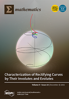
A rectifying curve is a twisted curve with the property that all of its rectifying planes pass through a fixed point. If this point is the origin of the Cartesian coordinate system, then the position vector of the rectifying curve always lies in the rectifying plane. A remarkable property of these curves is that the ratio between torsion and curvature is a nonconstant linear function of the arc-length parameter. In this paper, we give a new characterization of rectifying curves; namely, we prove that a curve is a rectifying curve if and only if it has a spherical involute. Consequently, rectifying curves can be constructed as evolutes of spherical twisted curves. We express the curvature and the torsion of a rectifying spherical curve and give the necessary and sufficient conditions for a curve and its involute to be both rectifying curves. View this paper.
  • Issues are regarded as officially published after their release is announced to the table of contents alert mailing list.
  • You may sign up for e-mail alerts to receive table of contents of newly released issues.
  • PDF is the official format for papers published in both, html and pdf forms. To view the papers in pdf format, click on the "PDF Full-text" link, and use the free Adobe Reader to open them.
Order results
Result details
Section
Select all
Export citation of selected articles as:
12 pages, 296 KiB  
Article
On the Packing Partitioning Problem on Directed Graphs
by Babak Samadi and Ismael G. Yero
Mathematics 2021, 9(23), 3148; https://doi.org/10.3390/math9233148 - 6 Dec 2021
Viewed by 1788
Abstract
This work is aimed to continue studying the packing sets of digraphs via the perspective of partitioning the vertex set of a digraph into packing sets (which can be interpreted as a type of vertex coloring of digraphs) and focused on finding the [...] Read more.
This work is aimed to continue studying the packing sets of digraphs via the perspective of partitioning the vertex set of a digraph into packing sets (which can be interpreted as a type of vertex coloring of digraphs) and focused on finding the minimum cardinality among all packing partitions for a given digraph D, called the packing partition number of D. Some lower and upper bounds on this parameter are proven, and their exact values for directed trees are given in this paper. In the case of directed trees, the proof results in a polynomial-time algorithm for finding a packing partition of minimum cardinality. We also consider this parameter in digraph products. In particular, a complete solution to this case is presented when dealing with the rooted products. Full article
(This article belongs to the Section Mathematics and Computer Science)
13 pages, 447 KiB  
Article
On g-Noncommuting Graph of a Finite Group Relative to Its Subgroups
by Monalisha Sharma, Rajat Kanti Nath and Yilun Shang
Mathematics 2021, 9(23), 3147; https://doi.org/10.3390/math9233147 - 6 Dec 2021
Cited by 6 | Viewed by 2130
Abstract
Let H be a subgroup of a finite non-abelian group G and gG. Let Z(H,G)={xH:xy=yx,yG}. We introduce [...] Read more.
Let H be a subgroup of a finite non-abelian group G and gG. Let Z(H,G)={xH:xy=yx,yG}. We introduce the graph ΔH,Gg whose vertex set is G\Z(H,G) and two distinct vertices x and y are adjacent if xH or yH and [x,y]g,g1, where [x,y]=x1y1xy. In this paper, we determine whether ΔH,Gg is a tree among other results. We also discuss about its diameter and connectivity with special attention to the dihedral groups. Full article
Show Figures

Figure 1

Figure 1
<p><math display="inline"><semantics> <msubsup> <mo>Δ</mo> <mrow> <msub> <mi>H</mi> <mn>1</mn> </msub> <mo>,</mo> <msub> <mi>A</mi> <mn>4</mn> </msub> </mrow> <mrow> <mi>b</mi> <mi>a</mi> <msup> <mi>b</mi> <mn>2</mn> </msup> </mrow> </msubsup> </semantics></math>.</p>
Full article ">Figure 2
<p><math display="inline"><semantics> <msubsup> <mo>Δ</mo> <mrow> <msub> <mi>H</mi> <mn>1</mn> </msub> <mo>,</mo> <msub> <mi>A</mi> <mn>4</mn> </msub> </mrow> <mrow> <msup> <mi>b</mi> <mn>2</mn> </msup> <mi>a</mi> <mi>b</mi> </mrow> </msubsup> </semantics></math>.</p>
Full article ">Figure 3
<p><math display="inline"><semantics> <msubsup> <mo>Δ</mo> <mrow> <msub> <mi>H</mi> <mn>2</mn> </msub> <mo>,</mo> <msub> <mi>A</mi> <mn>4</mn> </msub> </mrow> <mi>a</mi> </msubsup> </semantics></math>.</p>
Full article ">Figure 4
<p><math display="inline"><semantics> <msubsup> <mo>Δ</mo> <mrow> <msub> <mi>H</mi> <mn>2</mn> </msub> <mo>,</mo> <msub> <mi>A</mi> <mn>4</mn> </msub> </mrow> <mrow> <msup> <mi>b</mi> <mn>2</mn> </msup> <mi>a</mi> <mi>b</mi> </mrow> </msubsup> </semantics></math>.</p>
Full article ">Figure 5
<p><math display="inline"><semantics> <msubsup> <mo>Δ</mo> <mrow> <msub> <mi>H</mi> <mn>3</mn> </msub> <mo>,</mo> <msub> <mi>A</mi> <mn>4</mn> </msub> </mrow> <mi>a</mi> </msubsup> </semantics></math>.</p>
Full article ">Figure 6
<p><math display="inline"><semantics> <msubsup> <mo>Δ</mo> <mrow> <msub> <mi>H</mi> <mn>3</mn> </msub> <mo>,</mo> <msub> <mi>A</mi> <mn>4</mn> </msub> </mrow> <mrow> <mi>b</mi> <mi>a</mi> <msup> <mi>b</mi> <mn>2</mn> </msup> </mrow> </msubsup> </semantics></math>.</p>
Full article ">
18 pages, 15168 KiB  
Article
Control Method for Flexible Joints in Manipulator Based on BP Neural Network Tuning PI Controller
by Hexu Yang, Xiaopeng Li, Jinchi Xu, Dongyang Shang and Xingchao Qu
Mathematics 2021, 9(23), 3146; https://doi.org/10.3390/math9233146 - 6 Dec 2021
Cited by 5 | Viewed by 2838
Abstract
With the development of robot technology, integrated joints with small volume and convenient installation have been widely used. Based on the double inertia system, an integrated joint motor servo system model considering gear angle error and friction interference is established, and a joint [...] Read more.
With the development of robot technology, integrated joints with small volume and convenient installation have been widely used. Based on the double inertia system, an integrated joint motor servo system model considering gear angle error and friction interference is established, and a joint control strategy based on BP neural network and pole assignment method is designed to suppress the vibration of the system. Firstly, the dynamic equation of a planetary gear system is derived based on the Lagrange method, and the gear vibration of angular displacement is calculated. Secondly, the vibration displacement of the sun gear is introduced into the motor servo system in the form of the gear angle error, and the double inertia system model including angle error and friction torque is established. Then, the PI controller parameters are determined by pole assignment method, and the PI parameters are adjusted in real time based on the BP neural network, which effectively suppresses the vibration of the system. Finally, the effects of friction torque, pole damping coefficient and control strategy on the system response and the effectiveness of vibration suppression are analyzed. Full article
Show Figures

Figure 1

Figure 1
<p>Schematic diagram of flexible joint with gears.</p>
Full article ">Figure 2
<p>Schematic diagram of flexible joint with gears.</p>
Full article ">Figure 3
<p>Schematic diagram of gear rotation error.</p>
Full article ">Figure 4
<p>Schematic diagram of meshing stiffness and gear backlash. (<b>a</b>) Schematic diagram of meshing stiffness (<b>b</b>) Schematic diagram of gear backlash.</p>
Full article ">Figure 5
<p>The control block diagram of the flexible joint servo system.</p>
Full article ">Figure 6
<p>The specific control flow of BP neural network.</p>
Full article ">Figure 7
<p>PI controller based on BP neural network.</p>
Full article ">Figure 8
<p>The structure of BP neural network.</p>
Full article ">Figure 9
<p>Control block diagram of the flexible joint servo system.</p>
Full article ">Figure 10
<p>The influence of friction torque on the system. (<b>a</b>) Image of friction torque (<b>b</b>) Influence of friction torque on required input torque. (<b>c</b>) Influence of friction torque on load speed (<b>d</b>) Influence of friction torque on load angle.</p>
Full article ">Figure 10 Cont.
<p>The influence of friction torque on the system. (<b>a</b>) Image of friction torque (<b>b</b>) Influence of friction torque on required input torque. (<b>c</b>) Influence of friction torque on load speed (<b>d</b>) Influence of friction torque on load angle.</p>
Full article ">Figure 11
<p>Simulation results under step signal. (<b>a</b>) Motor end speed output (<b>b</b>) Motor end angle output. (<b>c</b>) Load end speed output (<b>d</b>) Load end angle output.</p>
Full article ">Figure 11 Cont.
<p>Simulation results under step signal. (<b>a</b>) Motor end speed output (<b>b</b>) Motor end angle output. (<b>c</b>) Load end speed output (<b>d</b>) Load end angle output.</p>
Full article ">Figure 12
<p>Simulation results under sinusoidal signal. (<b>a</b>) Motor end speed output (<b>b</b>) Motor end angle output. (<b>c</b>) Load end speed output (<b>d</b>) Load end angle output.</p>
Full article ">Figure 13
<p>Motor output under different control strategies. (<b>a</b>) Rotation speed at the motor end. (<b>b</b>) Rotational speed error at the motor end.</p>
Full article ">Figure 14
<p>The load output under different control strategies. (<b>a</b>) Rotation speed at the load end. (<b>b</b>) Speed error at the load end.</p>
Full article ">
13 pages, 322 KiB  
Article
Norm Inflation for Benjamin–Bona–Mahony Equation in Fourier Amalgam and Wiener Amalgam Spaces with Negative Regularity
by Divyang G. Bhimani and Saikatul Haque
Mathematics 2021, 9(23), 3145; https://doi.org/10.3390/math9233145 - 6 Dec 2021
Cited by 5 | Viewed by 1906
Abstract
We consider the Benjamin–Bona–Mahony (BBM) equation of the form ut+ux+uuxuxxt=0,(x,t)M×R where M=T or R. We [...] Read more.
We consider the Benjamin–Bona–Mahony (BBM) equation of the form ut+ux+uuxuxxt=0,(x,t)M×R where M=T or R. We establish norm inflation (NI) with infinite loss of regularity at general initial data in Fourier amalgam and Wiener amalgam spaces with negative regularity. This strengthens several known NI results at zero initial data in Hs(T) established by Bona–Dai (2017) and the ill-posedness result established by Bona–Tzvetkov (2008) and Panthee (2011) in Hs(R). Our result is sharp with respect to the local well-posedness result of Banquet–Villamizar–Roa (2021) in modulation spaces Ms2,1(R) for s0. Full article
(This article belongs to the Special Issue Microlocal and Time-Frequency Analysis)
10 pages, 708 KiB  
Article
Attribute Service Performance Index Based on Poisson Process
by Kuen-Suan Chen, Chang-Hsien Hsu and Ting-Hsin Hsu
Mathematics 2021, 9(23), 3144; https://doi.org/10.3390/math9233144 - 6 Dec 2021
Cited by 3 | Viewed by 2481
Abstract
The purpose of a shop enhancing customer satisfaction is to raise its total revenue as the rate of customer purchases in the shop increases. Some studies have pointed out that the amount of customer arrival at a shop is a Poisson process. A [...] Read more.
The purpose of a shop enhancing customer satisfaction is to raise its total revenue as the rate of customer purchases in the shop increases. Some studies have pointed out that the amount of customer arrival at a shop is a Poisson process. A simple and easy-to-use evaluation index proposed for the Poisson process with the attribute characteristic will help various shops evaluate their business performance. In addition, developing an excellent and practical service performance evaluation method will be beneficial to the advancement of shop service quality as well as corporate image, thereby increasing the profitability and competitiveness of the shop. As the surroundings of the internet of things (IoT) are becoming gradually common and mature, various commercial data measurement and collection technologies are constantly being refined to form a huge amount of production data. Efficient data analysis and application can assist enterprises in making wise and efficient decisions within a short time. Thus, following the simple and easy-to-use principle, this paper proposes an attribute service performance index based on a Poisson process. Since the index had unknown parameters, this paper subsequently figured out the best estimator and used the central limit theorem to derive the confidence interval of the service efficiency index based on random samples. Then, we constructed the membership function based on the α-cuts of the triangular shaped fuzzy number. Finally, we came up with a fuzzy testing model based on the membership function to improve the accuracy of the test when the sample size is small in order to meet enterprises’ needs for quick responses as well as reducing the evaluation cost. Full article
(This article belongs to the Special Issue Fuzzy Applications in Industrial Engineering)
Show Figures

Figure 1

Figure 1
<p>Membership functions of <math display="inline"><semantics> <mrow> <mi>η</mi> <mo stretchy="false">(</mo> <mi>x</mi> <mo stretchy="false">)</mo> </mrow> </semantics></math> and <math display="inline"><semantics> <mrow> <msup> <mi>η</mi> <mo>′</mo> </msup> <mo stretchy="false">(</mo> <mi>x</mi> <mo stretchy="false">)</mo> </mrow> </semantics></math>.</p>
Full article ">Figure 2
<p>Membership functions of <math display="inline"><semantics> <mrow> <msup> <mi>η</mi> <mo>′</mo> </msup> <mo stretchy="false">(</mo> <mi>x</mi> <mo stretchy="false">)</mo> </mrow> </semantics></math> with <math display="inline"><semantics> <mrow> <msub> <mi>C</mi> <mn>0</mn> </msub> </mrow> </semantics></math> <math display="inline"><semantics> <mo>=</mo> </semantics></math> 0.896 and <math display="inline"><semantics> <mrow> <mi>η</mi> <mo stretchy="false">(</mo> <mi>x</mi> <mo stretchy="false">)</mo> </mrow> </semantics></math> with <math display="inline"><semantics> <mrow> <msubsup> <mi>S</mi> <mrow> <mi>λ</mi> <mn>0</mn> </mrow> <mo>*</mo> </msubsup> </mrow> </semantics></math> <math display="inline"><semantics> <mo>=</mo> </semantics></math> 0.900.</p>
Full article ">
26 pages, 651 KiB  
Article
A Continuous-Time Network Evolution Model Describing 2- and 3-Interactions
by István Fazekas and Attila Barta
Mathematics 2021, 9(23), 3143; https://doi.org/10.3390/math9233143 - 6 Dec 2021
Cited by 1 | Viewed by 2227
Abstract
A continuous-time network evolution model is considered. The evolution of the network is based on 2- and 3-interactions. 2-interactions are described by edges, and 3-interactions are described by triangles. The evolution of the edges and triangles is governed by a multi-type continuous-time branching [...] Read more.
A continuous-time network evolution model is considered. The evolution of the network is based on 2- and 3-interactions. 2-interactions are described by edges, and 3-interactions are described by triangles. The evolution of the edges and triangles is governed by a multi-type continuous-time branching process. The limiting behaviour of the network is studied by mathematical methods. We prove that the number of triangles and edges have the same magnitude on the event of non-extinction, and it is eαt, where α is the Malthusian parameter. The probability of the extinction and the degree process of a fixed vertex are also studied. The results are illustrated by simulations. Full article
(This article belongs to the Special Issue Stability Problems for Stochastic Models: Theory and Applications II)
Show Figures

Figure 1

Figure 1
<p>Example of the graph evolution model with parameter set: <math display="inline"><semantics> <mrow> <msub> <mi>r</mi> <mn>1</mn> </msub> <mo>=</mo> <mn>0.1</mn> <mo>,</mo> <mspace width="3.33333pt"/> <msub> <mi>p</mi> <mn>1</mn> </msub> <mo>=</mo> <mn>0.4</mn> <mo>,</mo> </mrow> </semantics></math> <math display="inline"><semantics> <mrow> <msub> <mi>p</mi> <mn>2</mn> </msub> <mo>=</mo> <mn>0.2</mn> <mo>,</mo> <mspace width="3.33333pt"/> <mi>b</mi> <mo>=</mo> <mn>0.1</mn> <mo>,</mo> <mspace width="3.33333pt"/> <mi>c</mi> <mo>=</mo> <mn>0.1</mn> </mrow> </semantics></math>.</p>
Full article ">Figure 2
<p>Examples of the graph evolution model with two different parameter sets.</p>
Full article ">Figure 3
<p>Measurements of a single process on a logarithmic scale.</p>
Full article ">Figure 4
<p>The average of 100 processes generated by the same parameter set and the regression line.</p>
Full article ">
15 pages, 1076 KiB  
Article
On Interval-Valued Fuzzy Soft Preordered Sets and Associated Applications in Decision-Making
by Mabruka Ali and Adem Kılıçman
Mathematics 2021, 9(23), 3142; https://doi.org/10.3390/math9233142 - 6 Dec 2021
Cited by 2 | Viewed by 1953
Abstract
Recently, using interval-valued fuzzy soft sets to rank alternatives has become an important research area in decision-making because it provides decision-makers with the best option in a vague and uncertain environment. The present study aims to give an extensive insight into decision-making processes [...] Read more.
Recently, using interval-valued fuzzy soft sets to rank alternatives has become an important research area in decision-making because it provides decision-makers with the best option in a vague and uncertain environment. The present study aims to give an extensive insight into decision-making processes relying on a preference relationship of interval-valued fuzzy soft sets. Firstly, interval-valued fuzzy soft preorderings and an interval-valued fuzzy soft equivalence are established based on the interval-valued fuzzy soft topology. Then, two crisp preordering sets, namely lower crisp and upper crisp preordering sets, are proposed. Next, a score function depending on comparison matrices is expressed in solving multi-group decision-making problems. Finally, a numerical example is given to illustrate the validity and efficacy of the proposed method. Full article
Show Figures

Figure 1

Figure 1
<p>The flowchart for Algorithm 1.</p>
Full article ">
18 pages, 3148 KiB  
Article
Application of Machine Learning Model for the Prediction of Settling Velocity of Fine Sediments
by Wing Son Loh, Ren Jie Chin, Lloyd Ling, Sai Hin Lai and Eugene Zhen Xiang Soo
Mathematics 2021, 9(23), 3141; https://doi.org/10.3390/math9233141 - 6 Dec 2021
Cited by 6 | Viewed by 2834
Abstract
Sedimentation management is one of the primary factors in achieving sustainable development of water resources. However, due to difficulties in conducting in-situ tests, and the complex nature of fine sediments, it remains a challenging task when dealing with issues related to settling velocity. [...] Read more.
Sedimentation management is one of the primary factors in achieving sustainable development of water resources. However, due to difficulties in conducting in-situ tests, and the complex nature of fine sediments, it remains a challenging task when dealing with issues related to settling velocity. Hence, the machine learning model appears as a suitable tool to predict the settling velocity of fine sediments in water bodies. In this study, three different machine learning-based models, namely, the radial basis function neural network (RBFNN), back propagation neural network (BPNN), and self-organizing feature map (SOFM), were developed with four hydraulic parameters, including the inlet depth, particle size, and the relative x and y particle positions. The five distinct statistical measures, consisting of the root mean square error (RMSE), Nash–Sutcliffe efficiency (NSE), mean absolute error (MAE), mean value accounted for (MVAF), and total variance explained (TVE), were used to assess the performance of the models. The SOFM with the 25 × 25 Kohonen map had shown superior results with RMSE of 0.001307, NSE of 0.7170, MAE of 0.000647, MVAF of 101.25%, and TVE of 71.71%. Full article
(This article belongs to the Special Issue Advances of Machine Learning and Their Applications)
Show Figures

Figure 1

Figure 1
<p>General network architecture of a typical ANN.</p>
Full article ">Figure 2
<p>Flowchart of research methodology.</p>
Full article ">Figure 3
<p>Network architecture of the proposed RBFNN.</p>
Full article ">Figure 4
<p>Network architecture of the proposed BPNN.</p>
Full article ">Figure 5
<p>Network architecture of the proposed SOFM.</p>
Full article ">Figure 6
<p>Comparison plot of predicted and observed settling velocity for the RBFNN model with network architecture 4-16-1.</p>
Full article ">Figure 7
<p>Comparison plot of predicted and observed settling velocity for the BPNN model with network architecture 4-7-1.</p>
Full article ">Figure 8
<p>Comparison plot of predicted and observed settling velocity for the SOFM model with a 25 × 25 Kohonen map.</p>
Full article ">Figure 9
<p>Codes plot of the 25 × 25 Kohonen map.</p>
Full article ">Figure 10
<p>Heat maps of the 25 × 25 Kohonen map.</p>
Full article ">Figure 11
<p>Residual plots of the three ANN models (RBFNN, BPNN, SOFM).</p>
Full article ">
20 pages, 305 KiB  
Article
Methods of Ensuring Invariance with Respect to External Disturbances: Overview and New Advances
by Aleksey Antipov, Svetlana Krasnova and Victor Utkin
Mathematics 2021, 9(23), 3140; https://doi.org/10.3390/math9233140 - 6 Dec 2021
Cited by 11 | Viewed by 1845
Abstract
In this paper, we carry out a demonstration and comparative analysis of known methods of the synthesis of various control laws ensuring the invariance of the output (controlled) variable with respect to external disturbances under various assumptions about their type and channels of [...] Read more.
In this paper, we carry out a demonstration and comparative analysis of known methods of the synthesis of various control laws ensuring the invariance of the output (controlled) variable with respect to external disturbances under various assumptions about their type and channels of acting on the control plant. Methods of the synthesis are presented on the example of a third-order nonlinear system with single input and single output (SISO-systems), dynamic feedback synthesis is presented at a descriptive level and the focus is on procedures of static feedback synthesis. For the systems in which the matching conditions are not satisfied, it is concluded that it is expedient to introduce smooth and bounded nonlinear local feedbacks. Within the framework of the block control principle, we developed an iterative procedure of synthesis of S-shaped sigmoid feedbacks for such systems. Nonlinear local feedbacks ensure stabilization of the output variable with the given accuracy and settling time as in a system with traditionally used linear local feedbacks with high gains. However, in contrast to it, sigmoid functions do not lead to a large overshoot of state variables and control actions. Full article
20 pages, 3204 KiB  
Article
Dynamical Analysis of a Navigation Algorithm
by Mireya Cabezas-Olivenza, Ekaitz Zulueta, Ander Sánchez-Chica, Adrian Teso-Fz-Betoño and Unai Fernandez-Gamiz
Mathematics 2021, 9(23), 3139; https://doi.org/10.3390/math9233139 - 6 Dec 2021
Cited by 9 | Viewed by 3278
Abstract
There is presently a need for more robust navigation algorithms for autonomous industrial vehicles. These have reasonably guaranteed the adequate reliability of the navigation. In the current work, the stability of a modified algorithm for collision-free guiding of this type of vehicle is [...] Read more.
There is presently a need for more robust navigation algorithms for autonomous industrial vehicles. These have reasonably guaranteed the adequate reliability of the navigation. In the current work, the stability of a modified algorithm for collision-free guiding of this type of vehicle is ensured. A lateral control and a longitudinal control are implemented. To demonstrate their viability, a stability analysis employing the Lyapunov method is carried out. In addition, this mathematical analysis enables the constants of the designed algorithm to be determined. In conjunction with the navigation algorithm, the present work satisfactorily solves the localization problem, also known as simultaneous localization and mapping (SLAM). Simultaneously, a convolutional neural network is managed, which is used to calculate the trajectory to be followed by the AGV, by implementing the artificial vision. The use of neural networks for image processing is considered to constitute the most robust and flexible method for realising a navigation algorithm. In this way, the autonomous vehicle is provided with considerable autonomy. It can be regarded that the designed algorithm is adequate, being able to trace any type of path. Full article
(This article belongs to the Special Issue State-of-the-Art Mathematical Applications in Europe)
Show Figures

Figure 1

Figure 1
<p>The AGV for which the algorithm is proposed.</p>
Full article ">Figure 2
<p>Schematic representation of the lateral control proposal.</p>
Full article ">Figure 3
<p>Positioning error vector and trajectory direction vector.</p>
Full article ">Figure 4
<p>Process of obtaining trajectory: (<b>a</b>) Image that AGV takes of the path; (<b>b</b>) Semantic segmentation of the path; (<b>c</b>) Medium point of the navigable mask; (<b>d</b>) Obtained path.</p>
Full article ">Figure 5
<p>Localization data for the AGV from image.</p>
Full article ">Figure 6
<p>Path approach: (<b>a</b>) Situation where <span class="html-italic">φ</span><sub>path</sub> is zero; (<b>b</b>) Situation where <span class="html-italic">φ</span><sub>path</sub> is not zero.</p>
Full article ">Figure 7
<p>Results of simulation: (<b>a</b>) Plot when <span class="html-italic">V</span> is high and <span class="html-italic">K</span><sub>1</sub> low; (<b>b</b>) Plot when <span class="html-italic">V</span> is low and <span class="html-italic">K</span><sub>1</sub> high.</p>
Full article ">Figure 8
<p>Results of the simulation: (<b>a</b>) The values of L in all the space; (<b>b</b>) The values of ΔL in all the space.</p>
Full article ">Figure 9
<p>The optimal value of <span class="html-italic">K</span><sub>2</sub>.</p>
Full article ">Figure 10
<p>Different path simulation: (<b>a</b>) Sinusoidal with AGV at the right side; (<b>b</b>) Sinusoidal with AGV at the left side; (<b>c</b>) Linear with AGV at the right side; (<b>d</b>) Linear with AGV at the left side; (<b>e</b>) Circular with AGV outside; (<b>f</b>) Circular with AGV inside.</p>
Full article ">Figure 10 Cont.
<p>Different path simulation: (<b>a</b>) Sinusoidal with AGV at the right side; (<b>b</b>) Sinusoidal with AGV at the left side; (<b>c</b>) Linear with AGV at the right side; (<b>d</b>) Linear with AGV at the left side; (<b>e</b>) Circular with AGV outside; (<b>f</b>) Circular with AGV inside.</p>
Full article ">Figure 11
<p>Positioning error values in a specific trajectory.</p>
Full article ">
16 pages, 2602 KiB  
Article
A New Method for Time Normalization Based on the Continuous Phase: Application to Neck Kinematics
by Carlos Llopis-Albert, William Ricardo Venegas Toro, Nidal Farhat, Pau Zamora-Ortiz and Álvaro Felipe Page Del Pozo
Mathematics 2021, 9(23), 3138; https://doi.org/10.3390/math9233138 - 5 Dec 2021
Cited by 2 | Viewed by 2899
Abstract
There is growing interest in analyzing human movement data for clinical, sport, and ergonomic applications. Functional Data Analysis (FDA) has emerged as an advanced statistical method for overcoming the shortcomings of traditional analytic methods, because the information about continuous signals can be assessed [...] Read more.
There is growing interest in analyzing human movement data for clinical, sport, and ergonomic applications. Functional Data Analysis (FDA) has emerged as an advanced statistical method for overcoming the shortcomings of traditional analytic methods, because the information about continuous signals can be assessed over time. This paper takes the current literature a step further by presenting a new time scale normalization method, based on the Hilbert transform, for the analysis of functional data and the assessment of the effect on the variability of human movement waveforms. Furthermore, a quantitative comparison of well-known methods for normalizing datasets of temporal biomechanical waveforms using functional data is carried out, including the linear normalization method and nonlinear registration methods of functional data. This is done using an exhaustive database of human neck flexion-extension movements, which encompasses 423 complete cycles of 31 healthy subjects measured in two trials of the experiment on different days. The results show the advantages of the novel method compared to existing techniques in terms of computational cost and the effectiveness of time-scale normalization on the phase differences of curves and on the amplitude of means, which are assessed by Root Mean Square (RMS) values of functional means of angles, angular velocities, and angular accelerations. Additionally, the confidence intervals are obtained through a bootstrapping process. Full article
(This article belongs to the Special Issue Mathematics, Statistics and Applied Computational Methods)
Show Figures

Figure 1

Figure 1
<p>Experimental setup.</p>
Full article ">Figure 2
<p>Absolute time-scale curves for angles (phi), velocities (Dphi), and accelerations (D2phi). To better appreciate the detail of the curves, only a quarter of the curves used in the analysis have been drawn, which have been chosen at random.</p>
Full article ">Figure 3
<p>Normalized angle (phi) curves for the four methods compared, together with their functional means (solid black line) and functional standard deviations (dashed black line).</p>
Full article ">Figure 4
<p>Normalized velocity (Dphi) curves for the four methods compared, together with their functional means (solid black line) and functional standard deviations (dashed black line).</p>
Full article ">Figure 5
<p>Normalized acceleration (D2phi) curves for the four methods compared, together with their functional means (solid black line) and functional standard deviations (dashed black line).</p>
Full article ">Figure 6
<p>Time warping functions for the four methods compared. To better appreciate the detail of the warping functions, only a quarter of the curves used in the analysis have been drawn (the same ones represented in <a href="#mathematics-09-03138-f002" class="html-fig">Figure 2</a>).</p>
Full article ">Figure 7
<p>Comparison of the time warping functions for the four methods and registration curve number #345.</p>
Full article ">
19 pages, 901 KiB  
Article
XCM: An Explainable Convolutional Neural Network for Multivariate Time Series Classification
by Kevin Fauvel, Tao Lin, Véronique Masson, Élisa Fromont and Alexandre Termier
Mathematics 2021, 9(23), 3137; https://doi.org/10.3390/math9233137 - 5 Dec 2021
Cited by 65 | Viewed by 8100
Abstract
Multivariate Time Series (MTS) classification has gained importance over the past decade with the increase in the number of temporal datasets in multiple domains. The current state-of-the-art MTS classifier is a heavyweight deep learning approach, which outperforms the second-best MTS classifier only on [...] Read more.
Multivariate Time Series (MTS) classification has gained importance over the past decade with the increase in the number of temporal datasets in multiple domains. The current state-of-the-art MTS classifier is a heavyweight deep learning approach, which outperforms the second-best MTS classifier only on large datasets. Moreover, this deep learning approach cannot provide faithful explanations as it relies on post hoc model-agnostic explainability methods, which could prevent its use in numerous applications. In this paper, we present XCM, an eXplainable Convolutional neural network for MTS classification. XCM is a new compact convolutional neural network which extracts information relative to the observed variables and time directly from the input data. Thus, XCM architecture enables a good generalization ability on both large and small datasets, while allowing the full exploitation of a faithful post hoc model-specific explainability method (Gradient-weighted Class Activation Mapping) by precisely identifying the observed variables and timestamps of the input data that are important for predictions. We first show that XCM outperforms the state-of-the-art MTS classifiers on both the large and small public UEA datasets. Then, we illustrate how XCM reconciles performance and explainability on a synthetic dataset and show that XCM enables a more precise identification of the regions of the input data that are important for predictions compared to the current deep learning MTS classifier also providing faithful explainability. Finally, we present how XCM can outperform the current most accurate state-of-the-art algorithm on a real-world application while enhancing explainability by providing faithful and more informative explanations. Full article
(This article belongs to the Special Issue Data Mining for Temporal Data Analysis)
Show Figures

Figure 1

Figure 1
<p>MTEX-CNN architecture. Abbreviations: <span class="html-italic">D</span>—number of observed variables, <span class="html-italic">de</span>—dense layer size, <span class="html-italic">F</span>—number of filters, <span class="html-italic">k</span>—kernel size and <span class="html-italic">T</span>—time series length.</p>
Full article ">Figure 2
<p>XCM architecture. Abbreviations: <span class="html-italic">BN</span>—Batch Normalization, <span class="html-italic">D</span>—number of observed variables, <span class="html-italic">F</span>—number of filters, <span class="html-italic">T</span>—time series length and <span class="html-italic">Window Size</span>—kernel size, which corresponds to the time window size.</p>
Full article ">Figure 3
<p>XCM average relative accuracy drop across the UEA datasets when using other time window sizes than the one used in the best configuration given in <a href="#mathematics-09-03137-t003" class="html-table">Table 3</a>. The performance drop is presented across four categories of datasets, defined according to XCM levels of accuracy shown in <a href="#mathematics-09-03137-t003" class="html-table">Table 3</a>. Abbreviation: Acc—Accuracy.</p>
Full article ">Figure 4
<p>Critical difference plot of the MTS classifiers on the UEA datasets with alpha equal to 0.05.</p>
Full article ">Figure 5
<p>Observed variables and time attribution maps supporting the correct MTEX-CNN and XCM predictions of an MTS from the synthetic dataset belonging to the class <span class="html-italic">Positive</span>. Abbreviation: Dim—Dimension.</p>
Full article ">Figure 6
<p>Observed variables and time attribution maps supporting the correct XCM prediction of an MTS from the real-world test set, which belongs to the class <span class="html-italic">Estrus</span>. The MTS sample is represented under the form of a heatmap with the regions important for the prediction highlighted with a red square.</p>
Full article ">Figure 7
<p>Parallel coordinates plot of XCM and the state-of-the-art MTS classifiers on the real-world application. Performance evaluation method: 5-fold cross-validation and an arithmetic mean of the F1-scores. As presented in <a href="#sec2dot2-mathematics-09-03137" class="html-sec">Section 2.2</a>, the models evaluated in the benchmark are: DTW<math display="inline"><semantics> <msub> <mrow/> <mi>D</mi> </msub> </semantics></math>, DTW<math display="inline"><semantics> <msub> <mrow/> <mi>I</mi> </msub> </semantics></math>, FCN, gRSF, LPS, MLSTM-FCN, MTEX-CNN, mv-ARF, ResNet, SMTS, UFS, WEASEL+MUSE and XCM.</p>
Full article ">
20 pages, 1807 KiB  
Article
E-Learning Platform Assessment and Selection Using Two-Stage Multi-Criteria Decision-Making Approach with Grey Theory: A Case Study in Vietnam
by Pham Ngoc Toan, Thanh-Tuan Dang and Le Thi Thu Hong
Mathematics 2021, 9(23), 3136; https://doi.org/10.3390/math9233136 - 5 Dec 2021
Cited by 21 | Viewed by 3971
Abstract
Education has changed dramatically due to the severe global pandemic COVID-19, with the phenomenal growth of e-learning, whereby teaching is undertaken remotely and on digital platforms. E-learning is revolutionizing education systems, as it remains the only option during the ongoing crisis and has [...] Read more.
Education has changed dramatically due to the severe global pandemic COVID-19, with the phenomenal growth of e-learning, whereby teaching is undertaken remotely and on digital platforms. E-learning is revolutionizing education systems, as it remains the only option during the ongoing crisis and has tremendous potential to fulfill instructional plans and safeguard students’ learning rights. The selection of e-learning platforms is a multi-criteria decision-making (MCDM) problem. Expert analyses over numerous criteria and alternatives are usually linguistic terms, which can be represented through grey numbers. This article proposes an integrated approach of grey analytic hierarchy process (G-AHP) and grey technique for order preference by similarity to ideal solution (G-TOPSIS) to evaluate the best e-learning website for network teaching. This introduced approach handles the linguistic evaluation of experts based on grey systems theory, estimates the relative importance of evaluation criteria with the G-AHP method, and acquires e-learning websites’ ranking utilizing G-TOPSIS. The applicability and superiority of the presented method are illustrated through a practical e-learning website selection case in Vietnam. From G-AHP analysis, educational level, price, right and understandable content, complete content, and up-to-date were found as the most impactful criteria. From G-TOPSIS, Edumall is the best platform. Comparisons are conducted with other MCDM methods; the priority orders of the best websites are similar, indicating the robust proposed methodology. The proposed integrated model in this study supports the stakeholders in selecting the most effective e-learning environments and could be a reference for further development of e-learning teaching-learning systems. Full article
(This article belongs to the Special Issue Decision Making and Its Applications)
Show Figures

Figure 1

Figure 1
<p>The concept of grey system theory.</p>
Full article ">Figure 2
<p>The research framework.</p>
Full article ">Figure 3
<p>The influence level of criteria from the G-AHP model.</p>
Full article ">Figure 4
<p>The decision tree for evaluation of e-learning websites.</p>
Full article ">Figure 5
<p>Final alternatives ranking of the G-TOPSIS model.</p>
Full article ">Figure 6
<p>Ranking results of the compared methods.</p>
Full article ">
24 pages, 7281 KiB  
Article
Prediction of Hydraulic Jumps on a Triangular Bed Roughness Using Numerical Modeling and Soft Computing Methods
by Mehdi Dasineh, Amir Ghaderi, Mohammad Bagherzadeh, Mohammad Ahmadi and Alban Kuriqi
Mathematics 2021, 9(23), 3135; https://doi.org/10.3390/math9233135 - 5 Dec 2021
Cited by 21 | Viewed by 3160
Abstract
This study investigates the characteristics of free and submerged hydraulic jumps on the triangular bed roughness in various T/I ratios (i.e., height and distance of roughness) using CFD modeling techniques. The accuracy of numerical modeling outcomes was checked and compared using [...] Read more.
This study investigates the characteristics of free and submerged hydraulic jumps on the triangular bed roughness in various T/I ratios (i.e., height and distance of roughness) using CFD modeling techniques. The accuracy of numerical modeling outcomes was checked and compared using artificial intelligence methods, namely Support Vector Machines (SVM), Gene Expression Programming (GEP), and Random Forest (RF). The results of the FLOW-3D® model and experimental data showed that the overall mean value of relative error is 4.1%, which confirms the numerical model’s ability to predict the characteristics of the free and submerged jumps. The SVM model with a minimum of Root Mean Square Error (RMSE) and a maximum of correlation coefficient (R2), compared with GEP and RF models in the training and testing phases for predicting the sequent depth ratio (y2/y1), submerged depth ratio (y3/y1), tailwater depth ratio (y4/y1), length ratio of jumps (Lj/y2*) and energy dissipation (ΔE/E1), was recognized as the best model. Moreover, the best result for predicting the length ratio of free jumps (Ljf/y2*) in the optimal gamma is γ = 10 and the length ratio of submerged jumps (Ljs/y2*) is γ = 0.60. Based on sensitivity analysis, the Froude number has the greatest effect on predicting the (y3/y1) compared with submergence factors (SF) and T/I. By omitting this parameter, the prediction accuracy is significantly reduced. Finally, the relationships with good correlation coefficients for the mentioned parameters in free and submerged jumps were presented based on numerical results. Full article
(This article belongs to the Special Issue Computational Optimizations for Machine Learning)
Show Figures

Figure 1

Figure 1
<p>Definition sketch of the free and submerged hydraulic jumps on a triangular bed roughness after Ghaderi et al. [<a href="#B26-mathematics-09-03135" class="html-bibr">26</a>].</p>
Full article ">Figure 2
<p>The boundary conditions governing the simulation, (<b>a</b>) smooth bed, (<b>b</b>) the triangular bed roughness.</p>
Full article ">Figure 3
<p>CFD flow discharge time variation in the inlet and outlet boundaries, (<b>a</b>) <span class="html-italic">Q</span> = 0.03 m<sup>3</sup>/s, (<b>b</b>) <span class="html-italic">Q</span> = 0.045 m<sup>3</sup>/s.</p>
Full article ">Figure 4
<p>Structured rectangular hexahedral mesh with two different mesh blocks, (<b>a</b>) smooth bed, (<b>b</b>) the triangular bed roughness.</p>
Full article ">Figure 5
<p>Variations of the relative error of <span class="html-italic">y</span><sub>3</sub>/<span class="html-italic">y</span><sub>1</sub> and <span class="html-italic">y</span><sub>2</sub>/<span class="html-italic">y</span><sub>1</sub> at <span class="html-italic">Fr</span><sub>1</sub> versus cell size.</p>
Full article ">Figure 6
<p>Schematic of the Support Vector Machine (SVM).</p>
Full article ">Figure 7
<p>Schematic of the Gene Expression Programming (GEP).</p>
Full article ">Figure 8
<p>Performance of Random Forest (RF).</p>
Full article ">Figure 9
<p>Numerical versus basic experimental parameters of submerged and free hydraulic jumps. (<b>a</b>) <span class="html-italic">y</span><sub>3</sub>/<span class="html-italic">y</span><sub>1</sub>, (<b>b</b>) <span class="html-italic">y</span><sub>4</sub>/<span class="html-italic">y</span><sub>1</sub>, (<b>c</b>) <span class="html-italic">L<sub>js</sub></span>/<span class="html-italic">y<sub>1</sub></span>, and (<b>d</b>) <span class="html-italic">y</span><sub>2</sub>/<span class="html-italic">y</span><sub>1</sub>.</p>
Full article ">Figure 10
<p>FLOW-3D<sup>®</sup> model versus SVM model predicted for the <span class="html-italic">y</span><sub>2</sub>/<span class="html-italic">y</span><sub>1</sub>.</p>
Full article ">Figure 11
<p>Comparison of FLOW-3D<sup>®</sup> model and SVM model for estimating the <span class="html-italic">y</span><sub>2</sub>/<span class="html-italic">y</span><sub>1</sub>.</p>
Full article ">Figure 12
<p>Comparison of the numerical results and the predicted models of (<span class="html-italic">y</span><sub>3</sub>/<span class="html-italic">y</span><sub>1</sub>) for the testing phase.</p>
Full article ">Figure 13
<p>Comparison of the numerical results and the predicted models of (<span class="html-italic">y</span><sub>4</sub>/<span class="html-italic">y</span><sub>1</sub>) for the testing phase.</p>
Full article ">Figure 14
<p>Variations R<sup>2</sup> and RMSE versus gamma for the best SVM model in jump length estimation.</p>
Full article ">Figure 15
<p>Comparison of FLOW-3D<sup>®</sup> and SVM model values to estimate the <math display="inline"><semantics> <mrow> <msub> <mi>L</mi> <mrow> <mi>j</mi> <mi>f</mi> </mrow> </msub> <mo>/</mo> <msubsup> <mi>y</mi> <mn>2</mn> <mo>*</mo> </msubsup> </mrow> </semantics></math>.</p>
Full article ">Figure 16
<p>Comparison of FLOW-3D<sup>®</sup> and SVM model values to estimate the <math display="inline"><semantics> <mrow> <msub> <mi>L</mi> <mrow> <mi>j</mi> <mi>s</mi> </mrow> </msub> <mo>/</mo> <msubsup> <mi>y</mi> <mn>2</mn> <mo>*</mo> </msubsup> </mrow> </semantics></math>.</p>
Full article ">Figure 17
<p>Radar graphs of R<sup>2</sup> and RMSE for energy dissipation due to free and submerged jumps in the testing phase.</p>
Full article ">Figure 18
<p>FLOW-3D<sup>®</sup> model versus SVM predicted for the free jump.</p>
Full article ">Figure 19
<p>FLOW-3D<sup>®</sup> model versus SVM predicted for the submerged jump.</p>
Full article ">
13 pages, 659 KiB  
Article
Study of Dynamics of a COVID-19 Model for Saudi Arabia with Vaccination Rate, Saturated Treatment Function and Saturated Incidence Rate
by Rubayyi T. Alqahtani and Abdelhamid Ajbar
Mathematics 2021, 9(23), 3134; https://doi.org/10.3390/math9233134 - 5 Dec 2021
Cited by 5 | Viewed by 3119
Abstract
This paper proposes, validates and analyzes the dynamics of the susceptible exposed infectious recovered (SEIR) model for the propagation of COVID-19 in Saudi Arabia, which recorded the largest number of cases in the Arab world. The model incorporates a saturated incidence rate, a [...] Read more.
This paper proposes, validates and analyzes the dynamics of the susceptible exposed infectious recovered (SEIR) model for the propagation of COVID-19 in Saudi Arabia, which recorded the largest number of cases in the Arab world. The model incorporates a saturated incidence rate, a constant vaccination rate and a nonlinear treatment function. The rate of treatment is assumed to be proportional to the number of infected persons when this number is low and reaches a fixed value for large number of infected individuals. The expression of the basic reproduction number is derived, and the model basic stability properties are studied. We show that when the basic reproduction number is less than one the model can predict both a Hopf and backward bifurcations. Simulations are also provided to fit the model to COVID-19 data in Saudi Arabia and to study the effects of the parameters of the treatment function and vaccination rate on disease control. Full article
(This article belongs to the Special Issue New Trends and Developments in Numerical Analysis)
Show Figures

Figure 1

Figure 1
<p>Block diagram of the model. The arrows show progression from one compartment to the next.</p>
Full article ">Figure 2
<p>Validation of the model using COVID-19 data in Saudi Arabia for a period of 180 days starting from 24 March 2021. Red line (actual data); Blue solid line (model predictions). (<b>a</b>) Infected cases; (<b>b</b>) Recovered cases.</p>
Full article ">Figure 3
<p>(<b>a</b>) Backward bifurcation. (<b>b</b>) Forward bifurcation. Solid line (stable branch); dashed line (unstable branch); LP (static limit point); HB (Hopf point); blue line (endemic equilibrium); and red line (disease free equilibrium).</p>
Full article ">Figure 3 Cont.
<p>(<b>a</b>) Backward bifurcation. (<b>b</b>) Forward bifurcation. Solid line (stable branch); dashed line (unstable branch); LP (static limit point); HB (Hopf point); blue line (endemic equilibrium); and red line (disease free equilibrium).</p>
Full article ">Figure 4
<p>Effect of the model parameters on the location of the Hopf point. (<b>a</b>) Effect of saturation factor (<b>b</b>); (<b>b</b>) Effect of maximal supplied medical resources (<b>c</b>).</p>
Full article ">Figure 5
<p>Effect of vaccination rate on the number of: (<b>a</b>) recovered cases and (<b>b</b>) susceptible cases.</p>
Full article ">Figure 5 Cont.
<p>Effect of vaccination rate on the number of: (<b>a</b>) recovered cases and (<b>b</b>) susceptible cases.</p>
Full article ">
25 pages, 867 KiB  
Article
Stability Analysis of Parameter Varying Genetic Toggle Switches Using Koopman Operators
by Jamiree Harrison and Enoch Yeung
Mathematics 2021, 9(23), 3133; https://doi.org/10.3390/math9233133 - 5 Dec 2021
Cited by 5 | Viewed by 3120
Abstract
The genetic toggle switch is a well known model in synthetic biology that represents the dynamic interactions between two genes that repress each other. The mathematical models for the genetic toggle switch that currently exist have been useful in describing circuit dynamics in [...] Read more.
The genetic toggle switch is a well known model in synthetic biology that represents the dynamic interactions between two genes that repress each other. The mathematical models for the genetic toggle switch that currently exist have been useful in describing circuit dynamics in rapidly dividing cells, assuming fixed or time-invariant kinetic rates. There is a growing interest in being able to model and extend synthetic biological function for growth conditions such as stationary phase or during nutrient starvation. As cells transition from one growth phase to another, kinetic rates become time-varying parameters. In this paper, we propose a novel class of parameter varying nonlinear models that can be used to describe the dynamics of genetic circuits, including the toggle switch, as they transition from different phases of growth. We show that there exists unique solutions for this class of systems, as well as for a class of systems that incorporates the microbial phenomena of quorum sensing. Further, we show that the domain of these systems, which is the positive orthant, is positively invariant. We also showcase a theoretical control strategy for these systems that would grant asymptotic monostability of a desired fixed point. We then take the general form of these systems and analyze their stability properties through the framework of time-varying Koopman operator theory. A necessary condition for asymptotic stability is also provided as well as a sufficient condition for instability. A Koopman control strategy for the system is also proposed, as well as an analogous discrete time-varying Koopman framework for applications with regularly sampled measurements. Full article
(This article belongs to the Special Issue Dynamical Systems and Operator Theory)
Show Figures

Figure 1

Figure 1
<p>Mutual repression between two genes in a toggle switch. Here, we see that the gene <span class="html-italic">x</span> represses the expression of gene <span class="html-italic">y</span>, and vice versa.</p>
Full article ">Figure 2
<p>Activation-repression network for GTSQS. Here we see that gene <span class="html-italic">x</span> represses the expression of gene <span class="html-italic">y</span>, and that gene <span class="html-italic">y</span> represses the expression of gene <span class="html-italic">x</span>. We also have that the quorum sensing activation response <span class="html-italic">z</span> activates the transcription of gene <span class="html-italic">x</span>. The inducers <math display="inline"><semantics> <msub> <mi>u</mi> <mn>1</mn> </msub> </semantics></math> and <math display="inline"><semantics> <msub> <mi>u</mi> <mn>2</mn> </msub> </semantics></math> represent inducers of their respective genes. The input <math display="inline"><semantics> <msub> <mi>u</mi> <mn>3</mn> </msub> </semantics></math> is the quantity of the molecule used by the microbe to detect the presence of other microbes.</p>
Full article ">Figure 3
<p>Simulated phase space of GTSQS with no input in accordance with the example system in (<a href="#FD7-mathematics-09-03133" class="html-disp-formula">7</a>). Trajectories are plotted with initial conditions as blue empty circles and fixed points are seen as red filled circles.</p>
Full article ">Figure 4
<p>Simulated phase space of GTSQS with input <math display="inline"><semantics> <mrow> <msub> <mi>u</mi> <mn>1</mn> </msub> <mo>=</mo> <mn>0</mn> <mo>,</mo> <mo> </mo> <msub> <mi>u</mi> <mn>2</mn> </msub> <mo>=</mo> <mn>0</mn> <mo>,</mo> <mo> </mo> <msub> <mi>u</mi> <mn>3</mn> </msub> <mo>=</mo> <mn>0.01</mn> </mrow> </semantics></math> in accordance with the example system in (<a href="#FD7-mathematics-09-03133" class="html-disp-formula">7</a>). Trajectories are plotted with initial conditions as blue empty circles and fixed points are seen as red filled circles.</p>
Full article ">
29 pages, 396 KiB  
Article
Determination of Bounds for the Jensen Gap and Its Applications
by Hidayat Ullah, Muhammad Adil Khan and Tareq Saeed
Mathematics 2021, 9(23), 3132; https://doi.org/10.3390/math9233132 - 5 Dec 2021
Cited by 17 | Viewed by 3282
Abstract
The Jensen inequality has been reported as one of the most consequential inequalities that has a lot of applications in diverse fields of science. For this reason, the Jensen inequality has become one of the most discussed developmental inequalities in the current literature [...] Read more.
The Jensen inequality has been reported as one of the most consequential inequalities that has a lot of applications in diverse fields of science. For this reason, the Jensen inequality has become one of the most discussed developmental inequalities in the current literature on mathematical inequalities. The main intention of this article is to find some novel bounds for the Jensen difference while using some classes of twice differentiable convex functions. We obtain the proposed bounds by utilizing the power mean and Höilder inequalities, the notion of convexity and the prominent Jensen inequality for concave function. We deduce several inequalities for power and quasi-arithmetic means as a consequence of main results. Furthermore, we also establish different improvements for Hölder inequality with the help of obtained results. Moreover, we present some applications of the main results in information theory. Full article
(This article belongs to the Special Issue Advances in Mathematical Inequalities and Applications)
20 pages, 11127 KiB  
Article
An Efficient Visually Meaningful Quantum Walks-Based Encryption Scheme for Secure Data Transmission on IoT and Smart Applications
by Ahmed A. Abd El-Latif, Abdullah M. Iliyasu and Bassem Abd-El-Atty
Mathematics 2021, 9(23), 3131; https://doi.org/10.3390/math9233131 - 4 Dec 2021
Cited by 5 | Viewed by 1999
Abstract
Smart systems and technologies have become integral parts of modern society. Their ubiquity makes it paramount to prioritise securing the privacy of data transferred between smart devices. Visual encryption is a technique employed to obscure images by rendering them meaningless to evade attention [...] Read more.
Smart systems and technologies have become integral parts of modern society. Their ubiquity makes it paramount to prioritise securing the privacy of data transferred between smart devices. Visual encryption is a technique employed to obscure images by rendering them meaningless to evade attention during transmission. However, the astounding computing power ascribed to quantum technology implies that even the best visually encrypted systems can be effortlessly violated. Consequently, the physical realisation quantum hardware portends great danger for visually encrypted date on smart systems. To circumvent this, our study proposes the integration of quantum walks (QWs) as a cryptographic mechanism to forestall violation of the integrity of images on smart systems. Specifically, we use QW first to substitute the original image and to subsequently permutate and embed it onto the reference image. Based on this structure, our proposed quantum walks visually meaningful cryptosystem facilities confidential transmission of visual information. Simulation-based experiments validate the performance of the proposed system in terms of visual quality, efficiency, robustness, and key space sensitivity, and by that, its potential to safeguard smart systems now and as we transition to the quantum era. Full article
Show Figures

Figure 1

Figure 1
<p>Illustration of framework for secure data on smart systems based on quantum walks.</p>
Full article ">Figure 2
<p>The outline of the presented visually encryption approach.</p>
Full article ">Figure 3
<p>Original images (<b>a</b>–<b>f</b>) each of size 256 × 256 used to validate the proposed scheme.</p>
Full article ">Figure 4
<p>Reference images (<b>a</b>–<b>d</b>) each of size 512 × 512 used to validate the proposed scheme.</p>
Full article ">Figure 5
<p>Outcomes of simulation tests for pairings of original and reference colour images in the dataset presented earlier in <a href="#mathematics-09-03131-f003" class="html-fig">Figure 3</a> and <a href="#mathematics-09-03131-f004" class="html-fig">Figure 4</a>. The original images are presented in the first row (<b>a</b>–<b>c</b>), while their encrypted versions with the Peppers (RImg01) image as reference image are presented in the second row (<b>d</b>–<b>f</b>). Third row (<b>g</b>–<b>i</b>), presents histograms of the encrypted versions of these images. Similarly, the fourth row (<b>j</b>–<b>l</b>) presents encrypted versions of the original images with Lake (RIm02) image as reference image, and their respective histograms are presented in the last row (<b>m</b>–<b>o</b>).</p>
Full article ">Figure 6
<p>Outcomes of simulation tests for pairings of original and reference greyscale images in the dataset presented earlier in <a href="#mathematics-09-03131-f003" class="html-fig">Figure 3</a> and <a href="#mathematics-09-03131-f004" class="html-fig">Figure 4</a>. The original images are presented in the first row (<b>a</b>–<b>c</b>), while their encrypted versions with the Baboon (RImg03) image as reference image are presented in the second row (<b>d</b>–<b>f</b>). Third row (<b>g</b>–<b>i</b>) presents histograms of the encrypted versions of these images. Similarly, the fourth row (<b>j</b>–<b>l</b>) presents encrypted versions of the original images with Plane (RIm04) image as reference image, and their respective histograms are presented in the last row (<b>m</b>–<b>o</b>).</p>
Full article ">Figure 7
<p>Histograms (<b>a</b>–<b>f</b>) for OImg01 and its encrypted version before embedding onto the reference.</p>
Full article ">Figure 8
<p>Histograms (<b>a</b>–<b>f</b>) for grayscale images and their encrypted version before embedding onto the reference.</p>
Full article ">Figure 9
<p>Correlation distribution (<b>a</b>–<b>i</b>) for encrypted image EImg01-1.</p>
Full article ">Figure 10
<p>Correlation distribution for OImg04 and its encrypted version before embedding onto the reference image.</p>
Full article ">Figure 11
<p>Outcomes of occlusion attacks (<b>e</b>–<b>h</b>) with various cut-outs of parts from the encrypted image EImg01-1 (<b>a</b>–<b>d</b>).</p>
Full article ">Figure 12
<p>Outcomes of noise attacks (<b>e</b>–<b>h</b>) with various Salt and Pepper (S&amp;P) noise intensities (<b>a</b>–<b>d</b>) appended to the encrypted image EImg01-1.</p>
Full article ">Figure 13
<p>Outcomes of decryption process for the encrypted image EImg01-1 using different values of key parameters. (<b>a</b>) Correct key. (<b>b</b>) Correct key except for N = 263. (<b>c</b>) Correct key except for S = 520. (<b>d</b>) Correct key except for <math display="inline"><semantics> <mi>β</mi> </semantics></math> = <math display="inline"><semantics> <mrow> <mi>π</mi> <mo>/</mo> <mn>3</mn> </mrow> </semantics></math>. (<b>e</b>) Correct key except for <math display="inline"><semantics> <msub> <mi>θ</mi> <mn>0</mn> </msub> </semantics></math> = <math display="inline"><semantics> <mrow> <mi>π</mi> <mo>/</mo> <mn>2</mn> </mrow> </semantics></math>. (<b>f</b>) Correct key except for <math display="inline"><semantics> <msub> <mi>θ</mi> <mn>1</mn> </msub> </semantics></math> = <math display="inline"><semantics> <mrow> <mi>π</mi> <mo>/</mo> <mn>2</mn> </mrow> </semantics></math>. (<b>g</b>) Correct key except for <math display="inline"><semantics> <msub> <mi>θ</mi> <mn>2</mn> </msub> </semantics></math> = <math display="inline"><semantics> <mrow> <mi>π</mi> <mo>/</mo> <mn>6</mn> </mrow> </semantics></math>. (<b>h</b>) Correct key except changing the first bit of <span class="html-italic">T</span> from 0 to 1. (<b>i</b>) Correct key except removing the last bit of <span class="html-italic">T</span>.</p>
Full article ">
18 pages, 1125 KiB  
Article
Early Prediction of DNN Activation Using Hierarchical Computations
by Bharathwaj Suresh, Kamlesh Pillai, Gurpreet Singh Kalsi, Avishaii Abuhatzera and Sreenivas Subramoney
Mathematics 2021, 9(23), 3130; https://doi.org/10.3390/math9233130 - 4 Dec 2021
Cited by 1 | Viewed by 2586
Abstract
Deep Neural Networks (DNNs) have set state-of-the-art performance numbers in diverse fields of electronics (computer vision, voice recognition), biology, bioinformatics, etc. However, the process of learning (training) from the data and application of the learnt information (inference) process requires huge computational resources. Approximate [...] Read more.
Deep Neural Networks (DNNs) have set state-of-the-art performance numbers in diverse fields of electronics (computer vision, voice recognition), biology, bioinformatics, etc. However, the process of learning (training) from the data and application of the learnt information (inference) process requires huge computational resources. Approximate computing is a common method to reduce computation cost, but it introduces loss in task accuracy, which limits their application. Using an inherent property of Rectified Linear Unit (ReLU), a popular activation function, we propose a mathematical model to perform MAC operation using reduced precision for predicting negative values early. We also propose a method to perform hierarchical computation to achieve the same results as IEEE754 full precision compute. Applying this method on ResNet50 and VGG16 shows that up to 80% of ReLU zeros (which is 50% of all ReLU outputs) can be predicted and detected early by using just 3 out of 23 mantissa bits. This method is equally applicable to other floating-point representations. Full article
(This article belongs to the Special Issue Computational Optimizations for Machine Learning)
Show Figures

Figure 1

Figure 1
<p>Example of the convolution operation. In this example, the stride is assumed to be 1. A <math display="inline"><semantics> <mrow> <mn>5</mn> <mo>×</mo> <mn>5</mn> </mrow> </semantics></math> output is produced from the <math display="inline"><semantics> <mrow> <mn>7</mn> <mo>×</mo> <mn>7</mn> </mrow> </semantics></math> input when a <math display="inline"><semantics> <mrow> <mn>3</mn> <mo>×</mo> <mn>3</mn> </mrow> </semantics></math> weight matrix is considered.</p>
Full article ">Figure 2
<p>Graphical representation of the ReLU function. If <span class="html-italic">x</span> is the input and <span class="html-italic">y</span> is the output, then <span class="html-italic">y</span> = 0 for <span class="html-italic">x</span> &lt; 0, and <span class="html-italic">y</span> = <span class="html-italic">x</span> for <span class="html-italic">x</span> ≥ 0.</p>
Full article ">Figure 3
<p>IEEE 754 floating point representation [<a href="#B54-mathematics-09-03130" class="html-bibr">54</a>]. The total bits are divided into sign, exponent, and mantissa. The single precision format has 1 sign, 8 exponents, and 23 mantissa bits, while the double precision has 1 sign, 11 exponents, and 52 mantissa bits.</p>
Full article ">Figure 4
<p>VGG-16 CNN architecture. There are 16 computation layers (13 convolution <math display="inline"><semantics> <mrow> <mo>−</mo> <mn>3</mn> <mo>×</mo> <mn>3</mn> </mrow> </semantics></math> kernel and three fully connected layers without dropout). Pooling layers are present in the intermediate stages to reduce the layer size as the network gets deeper. Regularization, normalization, and other layers may be present but have not been shown in this figure for simplicity.</p>
Full article ">Figure 5
<p>ResNet-50 Architecture. There are 50 computations layers (excluding convolution layers in the identity path) between the input and output. This includes 49 convolution layers and the fully-connected layer at the end. Res 2–1 (conv with 1 × 1, 64; 3 × 3, 64; 1 × 1, 256), Res 3–1 (1 × 1, 128; 3 × 3, 128; 1 × 1, 512) and Res 4–1 (1 × 1, 256; 3 × 3, 256; 1 × 1, 1024) are shown with a dotted boundary to indicate that they include a convolution layer along their identity path (also shown with a dotted boundary in the elaboration below without dropout). Regularization, normalization, and other layers may be present but have not been shown in this figure for simplicity.</p>
Full article ">Figure 6
<p>Flow chart depicting the steps to perform hierarchical compute (three steps) and detect ReLU zeros with reduced precision. The first step is to perform MAC using exponent and predict ReLU output; if undetermined, compute most significant 8-bits of mantissa and check ReLU again if still not conclusive perform compute using remaining mantissa bits (every next step uses previously computed values). Here, the red arrows depict writing to the memory, and blue arrows indicate read from memory. Black arrows indicate that the computation has been completed for the given input.</p>
Full article ">Figure 7
<p>Intuition behind estimating ReLU zeros based on reduced precision compute. In the hierarchical compute method, the value of “<span class="html-italic">n</span>” (number of MSB mantissa bits) is increased at each step, resulting in a decrease in the region of interest, until only positive values are remaining.</p>
Full article ">Figure 8
<p>Percentage of ReLU zeros present in (<b>a</b>) VGG16; (<b>b</b>) ResNet50 when a typical image is processed through the models. Only a few layers of ResNet-50 are shown for clarity—a similar trend is observed in all the layers.</p>
Full article ">Figure 9
<p>Distribution of ReLU inputs in different layers of ResNet-50. Here, Val is the input to the ReLU function. A total of 10 bins have been considered, and the range in each bin in mentioned in the figure. The different layers shown in the figure are: (<b>a</b>) first convolution layer from the input image (<b>b</b>) first convolution layer in the Res 1-1 block; (<b>c</b>) first convolution layer in the Res 2-1 block; (<b>d</b>) first convolution layer in the Res 3-1 block.</p>
Full article ">Figure 10
<p>Percentage of ReLU values detected using our model across different ResNet-50 layers. The first 33 convolution layers are shown in the figure. The number of MSB mantissa bits used were (<b>a</b>) 0; (<b>b</b>) 1; (<b>c</b>) 2; and (<b>d</b>) 3.</p>
Full article ">Figure 11
<p>Percentage of ReLU zeros identified by our model when different mantissa bits were considered. The figure shows the results in (<b>a</b>) Conv 1-2; (<b>b</b>) Conv 3-3; and (<b>c</b>) Conv 5-3 layers of VGG-16, and (<b>d</b>) second convolution layer of Res 1-1 block; (<b>e</b>) first convolution layer of Res 2-4 block; and (<b>f</b>) third convolution layer of Res 3-5 block. Similar results were observed in other layers of both ResNet-50 and VGG-16.</p>
Full article ">
18 pages, 3870 KiB  
Article
Continuous Stability TS Fuzzy Systems Novel Frame Controlled by a Discrete Approach and Based on SOS Methodology
by Ameni Ellouze, Omar Kahouli, Mohamed Ksantini, Ali Rebhi, Nidhal Hnaien and François Delmotte
Mathematics 2021, 9(23), 3129; https://doi.org/10.3390/math9233129 - 4 Dec 2021
Cited by 1 | Viewed by 1524
Abstract
Generally, the continuous and discrete TS fuzzy systems’ control is studied independently. Unlike the discrete systems, stability results for the continuous systems suffer from conservatism because it is still quite difficult to apply non-quadratic Lyapunov functions, something which is much easier for the [...] Read more.
Generally, the continuous and discrete TS fuzzy systems’ control is studied independently. Unlike the discrete systems, stability results for the continuous systems suffer from conservatism because it is still quite difficult to apply non-quadratic Lyapunov functions, something which is much easier for the discrete systems. In this paper and in order to obtain new results for the continuous case, we proposed to connect the continuous with the discrete cases and then check the stability of the continuous TS fuzzy systems by means of the discrete design approach. To this end, a novel frame was proposed using the sum of square approach (SOS) to check the stability of the continuous Takagi Sugeno (TS) fuzzy models based on the discrete controller. Indeed, the control of the continuous TS fuzzy models is ensured by the discrete gains obtained from the Euler discrete form and based on the non-quadratic Lyapunov function. The simulation examples applied for various models, by modifying the order of the Euler discrete fuzzy system, are presented to show the effectiveness of the proposed methodology. Full article
(This article belongs to the Special Issue Automatic Control and Soft Computing in Engineering)
Show Figures

Figure 1

Figure 1
<p>Stability regions using Theorem 1.</p>
Full article ">Figure 2
<p>Stability regions using Theorem 6 in Reference [<a href="#B28-mathematics-09-03129" class="html-bibr">28</a>].</p>
Full article ">Figure 3
<p>Stability regions using Theorem 10 in Reference [<a href="#B10-mathematics-09-03129" class="html-bibr">10</a>].</p>
Full article ">Figure 4
<p>Stability regions for <math display="inline"><semantics> <mrow> <mi>m</mi> <mo>=</mo> <mn>4</mn> </mrow> </semantics></math> and <math display="inline"><semantics> <mrow> <mi>δ</mi> <mo>=</mo> <mn>0.08</mn> </mrow> </semantics></math>.</p>
Full article ">Figure 5
<p>Stability regions for <math display="inline"><semantics> <mrow> <mi>m</mi> <mo>=</mo> <mn>10</mn> </mrow> </semantics></math> and <math display="inline"><semantics> <mrow> <mi>δ</mi> <mo>=</mo> <mn>0.2</mn> </mrow> </semantics></math>.</p>
Full article ">Figure 6
<p>Stability regions for <math display="inline"><semantics> <mrow> <mi>m</mi> <mo>=</mo> <mn>50</mn> </mrow> </semantics></math> and <math display="inline"><semantics> <mrow> <mi>δ</mi> <mo>=</mo> <mn>0.5</mn> </mrow> </semantics></math>.</p>
Full article ">Figure 7
<p>Stability regions for <math display="inline"><semantics> <mrow> <mi>m</mi> <mo>=</mo> <mn>100</mn> </mrow> </semantics></math> and <math display="inline"><semantics> <mrow> <mi>δ</mi> <mo>=</mo> <mn>0.4</mn> </mrow> </semantics></math>.</p>
Full article ">Figure 8
<p>Stability regions for <math display="inline"><semantics> <mrow> <mi>m</mi> <mo>=</mo> <mn>100</mn> </mrow> </semantics></math> and <math display="inline"><semantics> <mrow> <mi>δ</mi> <mo>=</mo> <mn>1.4</mn> </mrow> </semantics></math>.</p>
Full article ">Figure 9
<p>The state variables evolutions <math display="inline"><semantics> <mrow> <msub> <mi>x</mi> <mn>1</mn> </msub> <mo stretchy="false">(</mo> <mi>t</mi> <mo stretchy="false">)</mo> <mo>,</mo> <mo> </mo> <msub> <mi>x</mi> <mn>2</mn> </msub> <mo stretchy="false">(</mo> <mi>t</mi> <mo stretchy="false">)</mo> </mrow> </semantics></math> and the controller <math display="inline"><semantics> <mrow> <mi>u</mi> <mrow> <mo>(</mo> <mi>t</mi> <mo>)</mo> </mrow> </mrow> </semantics></math>.</p>
Full article ">Figure 10
<p>The state variables evolutions <math display="inline"><semantics> <mrow> <msub> <mi>x</mi> <mn>1</mn> </msub> <mo stretchy="false">(</mo> <mi>t</mi> <mo stretchy="false">)</mo> <mo>,</mo> <mo> </mo> <msub> <mi>x</mi> <mn>2</mn> </msub> <mo stretchy="false">(</mo> <mi>t</mi> <mo stretchy="false">)</mo> </mrow> </semantics></math> and the controller <math display="inline"><semantics> <mrow> <mi>u</mi> <mrow> <mo>(</mo> <mi>t</mi> <mo>)</mo> </mrow> </mrow> </semantics></math>.</p>
Full article ">Figure 11
<p>Regions stability for <math display="inline"><semantics> <mrow> <mi>m</mi> <mo>=</mo> <mn>10</mn> </mrow> </semantics></math> and <math display="inline"><semantics> <mrow> <mi>δ</mi> <mo>=</mo> <mn>0.2</mn> <mo> </mo> <mi mathvariant="normal">s</mi> </mrow> </semantics></math>.</p>
Full article ">Figure 12
<p>Regions stability for <math display="inline"><semantics> <mrow> <mi>m</mi> <mo>=</mo> <mn>50</mn> </mrow> </semantics></math> and <math display="inline"><semantics> <mrow> <mi>δ</mi> <mo>=</mo> <mn>0.2</mn> <mo> </mo> <mi mathvariant="normal">s</mi> </mrow> </semantics></math>.</p>
Full article ">Figure 13
<p>Regions stability for <math display="inline"><semantics> <mrow> <mi>m</mi> <mo>=</mo> <mn>100</mn> </mrow> </semantics></math> and <math display="inline"><semantics> <mrow> <mi>δ</mi> <mo>=</mo> <mn>0.4</mn> <mo> </mo> <mi mathvariant="normal">s</mi> </mrow> </semantics></math>.</p>
Full article ">Figure 14
<p>State variables evolution <math display="inline"><semantics> <mrow> <msub> <mi>x</mi> <mn>1</mn> </msub> <mo stretchy="false">(</mo> <mi>t</mi> <mo stretchy="false">)</mo> <mo>,</mo> <mo> </mo> <msub> <mi>x</mi> <mn>2</mn> </msub> <mo stretchy="false">(</mo> <mi>t</mi> <mo stretchy="false">)</mo> </mrow> </semantics></math> and the controller <math display="inline"><semantics> <mrow> <mi>u</mi> <mrow> <mo>(</mo> <mi>t</mi> <mo>)</mo> </mrow> </mrow> </semantics></math> (<math display="inline"><semantics> <mrow> <mi>a</mi> <mo>=</mo> <mn>60</mn> </mrow> </semantics></math>, <math display="inline"><semantics> <mrow> <mi>b</mi> <mo>=</mo> <mn>15</mn> </mrow> </semantics></math>, <math display="inline"><semantics> <mrow> <mi>m</mi> <mo>=</mo> <mn>100</mn> </mrow> </semantics></math>, and <math display="inline"><semantics> <mrow> <mi>δ</mi> <mo>=</mo> <mn>0.4</mn> </mrow> </semantics></math>).</p>
Full article ">Figure 15
<p>Evolution of the state variables <math display="inline"><semantics> <mrow> <msub> <mi>x</mi> <mn>1</mn> </msub> <mo stretchy="false">(</mo> <mi>t</mi> <mo stretchy="false">)</mo> <mo>,</mo> <mo> </mo> <msub> <mi>x</mi> <mn>2</mn> </msub> <mo stretchy="false">(</mo> <mi>t</mi> <mo stretchy="false">)</mo> </mrow> </semantics></math> and the controller <math display="inline"><semantics> <mrow> <mi>u</mi> <mrow> <mo>(</mo> <mi>t</mi> <mo>)</mo> </mrow> </mrow> </semantics></math> (<math display="inline"><semantics> <mrow> <mi>b</mi> <mo>=</mo> <mn>1</mn> </mrow> </semantics></math>, <math display="inline"><semantics> <mrow> <mi>a</mi> <mo>=</mo> <mo>−</mo> <mn>14</mn> </mrow> </semantics></math>, <math display="inline"><semantics> <mrow> <mi>m</mi> <mo>=</mo> <mn>50</mn> </mrow> </semantics></math>, and <math display="inline"><semantics> <mrow> <mi>δ</mi> <mo>=</mo> <mn>0.7</mn> <mo> </mo> <mi mathvariant="normal">s</mi> </mrow> </semantics></math>).</p>
Full article ">Figure 16
<p>The continuous closed loop curves for the model (25) controlled by the discrete law using <span class="html-italic">x</span>(0) = [−0.5, 0.5].</p>
Full article ">Figure 17
<p>The state evolution <math display="inline"><semantics> <mrow> <msub> <mstyle mathsize="140%" displaystyle="true"> <mi>x</mi> </mstyle> <mn>1</mn> </msub> <mrow> <mo>(</mo> <mi>t</mi> <mo>)</mo> </mrow> </mrow> </semantics></math> with σ = 0.014.</p>
Full article ">Figure 18
<p>The state evolution <math display="inline"><semantics> <mrow> <msub> <mstyle mathsize="140%" displaystyle="true"> <mi>x</mi> </mstyle> <mn>2</mn> </msub> <mrow> <mo>(</mo> <mi>t</mi> <mo>)</mo> </mrow> </mrow> </semantics></math> with σ = 0.03.</p>
Full article ">Figure 19
<p>The state evolutions <math display="inline"><semantics> <mrow> <msub> <mi>x</mi> <mn>1</mn> </msub> <mo stretchy="false">(</mo> <mi>t</mi> <mo stretchy="false">)</mo> <mo>,</mo> <mo> </mo> <msub> <mi>x</mi> <mn>2</mn> </msub> <mo stretchy="false">(</mo> <mi>t</mi> <mo stretchy="false">)</mo> </mrow> </semantics></math> with σ = 0.1.</p>
Full article ">
16 pages, 7844 KiB  
Article
Resolutions of the Jerk and Snap Vectors for a Quasi Curve in Euclidean 3-Space
by Ebrahem Hamouda, Clemente Cesarano, Sameh Askar and Ayman Elsharkawy
Mathematics 2021, 9(23), 3128; https://doi.org/10.3390/math9233128 - 4 Dec 2021
Cited by 6 | Viewed by 1606
Abstract
This work aims at studying resolutions of the jerk and snap vectors of a point particle moving along a quasi curve in Euclidean 3-space E3. In particular, we obtain the resolution of the jerk and snap vectors along the quasi vectors [...] Read more.
This work aims at studying resolutions of the jerk and snap vectors of a point particle moving along a quasi curve in Euclidean 3-space E3. In particular, we obtain the resolution of the jerk and snap vectors along the quasi vectors and offer an alternative resolution of the jerk and snap vectors along the tangential direction and two special radial directions that lie in the osculating and rectifying planes. This alternative resolution for a quasi plane curve in Euclidean 3-space E3 is given as corollary. Moreover, our results are illustrated via some examples. Full article
(This article belongs to the Special Issue Advanced Methods in Computational Mathematical Physics)
Show Figures

Figure 1

Figure 1
<p>The motion of point particle <math display="inline"><semantics> <mi mathvariant="script">P</mi> </semantics></math> along a quasi curve <math display="inline"><semantics> <mi>α</mi> </semantics></math> in <math display="inline"><semantics> <msup> <mi mathvariant="double-struck">E</mi> <mn>3</mn> </msup> </semantics></math>.</p>
Full article ">Figure 2
<p>The motion of point particle <math display="inline"><semantics> <mi mathvariant="script">P</mi> </semantics></math> along a quasi plane curve <math display="inline"><semantics> <mi>α</mi> </semantics></math> that contains a fixed origin <math display="inline"><semantics> <mi mathvariant="script">O</mi> </semantics></math>.</p>
Full article ">Figure 3
<p>The slant helix curve.</p>
Full article ">Figure 4
<p>The log-spiral curve.</p>
Full article ">
27 pages, 1580 KiB  
Article
Mixture of Species Sampling Models
by Federico Bassetti and Lucia Ladelli
Mathematics 2021, 9(23), 3127; https://doi.org/10.3390/math9233127 - 4 Dec 2021
Cited by 2 | Viewed by 1649
Abstract
We introduce mixtures of species sampling sequences (mSSS) and discuss how these sequences are related to various types of Bayesian models. As a particular case, we recover species sampling sequences with general (not necessarily diffuse) base measures. These models include some “spike-and-slab” non-parametric [...] Read more.
We introduce mixtures of species sampling sequences (mSSS) and discuss how these sequences are related to various types of Bayesian models. As a particular case, we recover species sampling sequences with general (not necessarily diffuse) base measures. These models include some “spike-and-slab” non-parametric priors recently introduced to provide sparsity. Furthermore, we show how mSSS arise while considering hierarchical species sampling random probabilities (e.g., the hierarchical Dirichlet process). Extending previous results, we prove that mSSS are obtained by assigning the values of an exchangeable sequence to the classes of a latent exchangeable random partition. Using this representation, we give an explicit expression of the Exchangeable Partition Probability Function of the partition generated by an mSSS. Some special cases are discussed in detail—in particular, species sampling sequences with general base measures and a mixture of species sampling sequences with Gibbs-type latent partition. Finally, we give explicit expressions of the predictive distributions of an mSSS. Full article
Show Figures

Figure 1

Figure 1
<p>Pictorial representation of the latent partition structure of an mSSS. In the example, the partition induced by <math display="inline"><semantics> <mrow> <mo>(</mo> <msub> <mi>ξ</mi> <mn>1</mn> </msub> <mo>,</mo> <mo>…</mo> <mo>,</mo> <msub> <mi>ξ</mi> <mi>n</mi> </msub> <mo>)</mo> </mrow> </semantics></math> for <math display="inline"><semantics> <mrow> <mi>n</mi> <mo>=</mo> <mn>8</mn> </mrow> </semantics></math> is <math display="inline"><semantics> <mrow> <msub> <mover accent="true"> <mo>Π</mo> <mo stretchy="false">˜</mo> </mover> <mi>n</mi> </msub> <mo>=</mo> <mrow> <mo>{</mo> <mrow> <mo>[</mo> <mn>1</mn> <mo>,</mo> <mn>3</mn> <mo>,</mo> <mn>4</mn> <mo>,</mo> <mn>7</mn> <mo>]</mo> </mrow> <mo>,</mo> <mrow> <mo>[</mo> <mn>2</mn> <mo>]</mo> </mrow> <mo>,</mo> <mrow> <mo>[</mo> <mn>5</mn> <mo>,</mo> <mn>6</mn> <mo>,</mo> <mn>8</mn> <mo>]</mo> </mrow> <mo>}</mo> </mrow> </mrow> </semantics></math>, and it is represented using rounded squares (left bottom). Circles at the top left represent a compatible latent partition, namely <math display="inline"><semantics> <mrow> <msub> <mo>Π</mo> <mi>n</mi> </msub> <mo>=</mo> <mrow> <mo>{</mo> <mrow> <mo>[</mo> <mn>1</mn> <mo>,</mo> <mn>3</mn> <mo>]</mo> </mrow> <mo>,</mo> <mrow> <mo>[</mo> <mn>2</mn> <mo>]</mo> </mrow> <mo>,</mo> <mrow> <mo>[</mo> <mn>4</mn> <mo>,</mo> <mn>7</mn> <mo>]</mo> </mrow> <mo>,</mo> <mrow> <mo>[</mo> <mn>5</mn> <mo>,</mo> <mn>8</mn> <mo>]</mo> </mrow> <mo>,</mo> <mrow> <mo>[</mo> <mn>6</mn> <mo>]</mo> </mrow> <mo>}</mo> </mrow> </mrow> </semantics></math>. The partition on <math display="inline"><semantics> <mrow> <mo>{</mo> <mn>1</mn> <mo>,</mo> <mo>…</mo> <mo>,</mo> <mn>5</mn> <mo>}</mo> </mrow> </semantics></math> induced by the latent <math display="inline"><semantics> <msubsup> <mi>Z</mi> <mi>n</mi> <mo>′</mo> </msubsup> </semantics></math>, i.e., <math display="inline"><semantics> <mrow> <msubsup> <mo>Π</mo> <mrow> <mrow> <mo>|</mo> </mrow> <msub> <mo>Π</mo> <mi>n</mi> </msub> <mrow> <mo>|</mo> </mrow> </mrow> <mrow> <mo>(</mo> <mn>0</mn> <mo>)</mo> </mrow> </msubsup> <mo>=</mo> <mrow> <mo>{</mo> <mrow> <mo>[</mo> <mn>1</mn> <mo>,</mo> <mn>3</mn> <mo>]</mo> </mrow> <mo>,</mo> <mrow> <mo>[</mo> <mn>2</mn> <mo>]</mo> </mrow> <mo>,</mo> <mrow> <mo>[</mo> <mn>4</mn> <mo>,</mo> <mn>5</mn> <mo>]</mo> </mrow> <mo>}</mo> </mrow> </mrow> </semantics></math>, is represented with squares in the middle of the figure. Combining <math display="inline"><semantics> <msub> <mo>Π</mo> <mi>n</mi> </msub> </semantics></math> and <math display="inline"><semantics> <msubsup> <mo>Π</mo> <mrow> <mrow> <mo>|</mo> </mrow> <msub> <mo>Π</mo> <mi>n</mi> </msub> <mrow> <mo>|</mo> </mrow> </mrow> <mrow> <mo>(</mo> <mn>0</mn> <mo>)</mo> </mrow> </msubsup> </semantics></math>, one obtains <math display="inline"><semantics> <msub> <mover accent="true"> <mo>Π</mo> <mo stretchy="false">˜</mo> </mover> <mi>n</mi> </msub> </semantics></math>. The statistics <math display="inline"><semantics> <mi mathvariant="bold-italic">n</mi> </semantics></math>, <math display="inline"><semantics> <mi mathvariant="bold-italic">m</mi> </semantics></math> and <math display="inline"><semantics> <mi>λ</mi> </semantics></math> corresponding to this particular configuration are shown in the box at the bottom right.</p>
Full article ">Figure 2
<p>Predictive CDFs for the relative changes in larcenies between 1991 and 1995 (relative to 1991) for the 90 most populous US counties; data taken from Section 2.1 of [<a href="#B34-mathematics-09-03127" class="html-bibr">34</a>]. Data have been rounded to the second decimal. Here, <math display="inline"><semantics> <mrow> <mi>n</mi> <mo>=</mo> <mn>90</mn> </mrow> </semantics></math> and <math display="inline"><semantics> <mrow> <mi>k</mi> <mo>=</mo> <mn>36</mn> </mrow> </semantics></math>. Solid line: empirical CDF. Dotted line: predictive CDF from (33). Dashed line: predictive CDF from PS2 with <math display="inline"><semantics> <mrow> <mi>H</mi> <mo>=</mo> <msub> <mi mathvariant="script">T</mi> <mrow> <mn>2</mn> <msub> <mi>α</mi> <mn>0</mn> </msub> </mrow> </msub> <mrow> <mo>(</mo> <mo>·</mo> <mo>|</mo> <msub> <mi>μ</mi> <mn>0</mn> </msub> <mo>,</mo> <msubsup> <mi>σ</mi> <mn>0</mn> <mn>2</mn> </msubsup> <mo>)</mo> </mrow> </mrow> </semantics></math>, <math display="inline"><semantics> <mrow> <msubsup> <mi>σ</mi> <mn>0</mn> <mn>2</mn> </msubsup> <mo>=</mo> <msub> <mi>β</mi> <mn>0</mn> </msub> <mrow> <mo>(</mo> <msub> <mi>k</mi> <mn>0</mn> </msub> <mo>+</mo> <mn>1</mn> <mo>)</mo> </mrow> <mo>/</mo> <msub> <mi>α</mi> <mn>0</mn> </msub> <msub> <mi>k</mi> <mn>0</mn> </msub> </mrow> </semantics></math>. Different plots correspond to different values of <math display="inline"><semantics> <mi>θ</mi> </semantics></math> and <math display="inline"><semantics> <mi>σ</mi> </semantics></math>. In all the plots, the predictive CDFs are evaluated with <math display="inline"><semantics> <mrow> <msub> <mi>μ</mi> <mn>0</mn> </msub> <mo>=</mo> <mn>0</mn> </mrow> </semantics></math>, <math display="inline"><semantics> <mrow> <msub> <mi>α</mi> <mn>0</mn> </msub> <mo>=</mo> <mn>0.1</mn> </mrow> </semantics></math>, <math display="inline"><semantics> <mrow> <msub> <mi>β</mi> <mn>0</mn> </msub> <mo>=</mo> <mn>0.1</mn> </mrow> </semantics></math> and <math display="inline"><semantics> <mrow> <msub> <mi>k</mi> <mn>0</mn> </msub> <mo>=</mo> <mn>0.1</mn> </mrow> </semantics></math>.</p>
Full article ">Figure 3
<p>Predictive CDFs for the relative changes in larcenies between 1991 and 1995 (relative to 1991) for the 90 most populous US counties; data taken from Section 2.1 of [<a href="#B34-mathematics-09-03127" class="html-bibr">34</a>]. Raw data, without rounding. Here, <math display="inline"><semantics> <mrow> <mi>n</mi> <mo>=</mo> <mn>90</mn> </mrow> </semantics></math> and <math display="inline"><semantics> <mrow> <mi>k</mi> <mo>=</mo> <mn>36</mn> </mrow> </semantics></math>. Solid line: empirical CDF. Dotted line: predictive CDF from (33). Dashed line: predictive CDF from PS2 with <math display="inline"><semantics> <mrow> <mi>H</mi> <mo>=</mo> <msub> <mi mathvariant="script">T</mi> <mrow> <mn>2</mn> <msub> <mi>α</mi> <mn>0</mn> </msub> </mrow> </msub> <mrow> <mo>(</mo> <mo>·</mo> <mo>|</mo> <msub> <mi>μ</mi> <mn>0</mn> </msub> <mo>,</mo> <msubsup> <mi>σ</mi> <mn>0</mn> <mn>2</mn> </msubsup> <mo>)</mo> </mrow> </mrow> </semantics></math>, <math display="inline"><semantics> <mrow> <msubsup> <mi>σ</mi> <mn>0</mn> <mn>2</mn> </msubsup> <mo>=</mo> <msub> <mi>β</mi> <mn>0</mn> </msub> <mrow> <mo>(</mo> <msub> <mi>k</mi> <mn>0</mn> </msub> <mo>+</mo> <mn>1</mn> <mo>)</mo> </mrow> <mo>/</mo> <msub> <mi>α</mi> <mn>0</mn> </msub> <msub> <mi>k</mi> <mn>0</mn> </msub> </mrow> </semantics></math>. Different plots correspond to different values of <math display="inline"><semantics> <mi>θ</mi> </semantics></math> and <math display="inline"><semantics> <mi>σ</mi> </semantics></math>. In all the plots, the predictive CDFs are evaluated with <math display="inline"><semantics> <mrow> <msub> <mi>μ</mi> <mn>0</mn> </msub> <mo>=</mo> <mn>0</mn> </mrow> </semantics></math>, <math display="inline"><semantics> <mrow> <msub> <mi>α</mi> <mn>0</mn> </msub> <mo>=</mo> <mn>0.1</mn> </mrow> </semantics></math>, <math display="inline"><semantics> <mrow> <msub> <mi>β</mi> <mn>0</mn> </msub> <mo>=</mo> <mn>0.1</mn> </mrow> </semantics></math> and <math display="inline"><semantics> <mrow> <msub> <mi>k</mi> <mn>0</mn> </msub> <mo>=</mo> <mn>0.1</mn> </mrow> </semantics></math>.</p>
Full article ">
19 pages, 2021 KiB  
Article
Enterprise Compensation System Statistical Modeling for Decision Support System Development
by Artur Mitsel, Aleksandr Shilnikov, Pavel Senchenko and Anatoly Sidorov
Mathematics 2021, 9(23), 3126; https://doi.org/10.3390/math9233126 - 4 Dec 2021
Cited by 3 | Viewed by 1857
Abstract
This article raises the issue of decision support system (DSS) development in enterprises concerning the compensation system (CS). The topic is relevant as the CS is one of the main components in human resource management in business. A key element of such DSSs [...] Read more.
This article raises the issue of decision support system (DSS) development in enterprises concerning the compensation system (CS). The topic is relevant as the CS is one of the main components in human resource management in business. A key element of such DSSs is CS models that provide predictive analytics. Such models are able to give information about how a particular CS affects output, product quality, employee satisfaction, and wage fund. Thus, the main goal of this article is to obtain a CS statistical model and its formulas for determining the probability densities of resultant indicators. To achieve this goal, the authors conducted several blocks of research. Firstly, mathematical formalization of CS functionality was described. Secondly, a statistical model of CS was built. Thirdly, calculations of CS result indicators were made. Reliable scientific methods were used: black box modeling and statistical modeling. This article proposes a statistical and analytical model. As an example, a piecework-bonus system statistical model is demonstrated. The discussion derives formulas of integral estimations showing the probability density of the resulting CS indicators and the related statistical characteristics. These results can be used to predict the behavior of the workforce. This constitutes the scientific novelty of the study, which will establish significant advances in the development of DSSs in the field of labor economics and HR management. Full article
Show Figures

Figure 1

Figure 1
<p>Description of the DSS modules.</p>
Full article ">Figure 2
<p>Black box model.</p>
Full article ">Figure 3
<p>The probability density plot—Q4.</p>
Full article ">Figure 4
<p>The probability of successfully reaching a set level of output.</p>
Full article ">Figure 5
<p>The probability density plot—G4.</p>
Full article ">Figure 6
<p>The probability of successfully reaching a set level of quality.</p>
Full article ">Figure 7
<p>The labor satisfaction (Sat4) probability density (<math display="inline"><semantics> <mrow> <mi>y</mi> <mn>1</mn> <mo>≤</mo> <mi>b</mi> <mn>2</mn> <mo stretchy="false">)</mo> </mrow> </semantics></math>.</p>
Full article ">Figure 8
<p>The labor satisfaction (Sat4) probability density (<math display="inline"><semantics> <mrow> <mi>y</mi> <mn>1</mn> <mo>&gt;</mo> <mi>b</mi> <mn>2</mn> </mrow> </semantics></math>).</p>
Full article ">
15 pages, 5484 KiB  
Article
Modelling of Heat Transfer Processes in Heat Exchangers for Cardiopulmonary Bypass
by Valentyna Danilova, Vladyslav Shlykov, Vitalii Kotovskyi, Nikolaj Višniakov and Andžela Šešok
Mathematics 2021, 9(23), 3125; https://doi.org/10.3390/math9233125 - 4 Dec 2021
Viewed by 2505
Abstract
A model of the heat exchange process in the heat exchanger of the cardiopulmonary bypass device is proposed which allows for automation of the process of temperature regulation in the cardiopulmonary bypass with an accuracy of ±1 °C during cardiac surgery under controlled [...] Read more.
A model of the heat exchange process in the heat exchanger of the cardiopulmonary bypass device is proposed which allows for automation of the process of temperature regulation in the cardiopulmonary bypass with an accuracy of ±1 °C during cardiac surgery under controlled cooling and warming of the patient’s heart and brain. The purpose of this research is to create a concept and model of the temperature control circuit using the MSC Easy5 system, the creation of mathematical models of blocks of the temperature control circuit, and the description of the principle of temperature control in the cardiopulmonary bypass circuit. The model of the temperature control loop in the heat exchanger of the heart-lung machine was created using the MSC Easy5 system with a programmable microcontroller. The microcontroller implements a specialized temperature control algorithm in the C language. The model allows the creation of a full-fledged virtual prototype of a temperature control device in a heat exchanger, and helps to conduct virtual tests of the developed device at the design stage. The model identifies control system flaws and influences decisions made before producing an official prototype of the product. Full article
(This article belongs to the Special Issue Applied Mathematical Modelling and Dynamical Systems)
Show Figures

Figure 1

Figure 1
<p>Application of the MSC Easy5 system for modelling the temperature control circuit in the CPB heat exchanger.</p>
Full article ">Figure 2
<p>Functional diagram of temperature control in heart-lung machine’s heat exchanger in the MSC Easy5 system.</p>
Full article ">Figure 3
<p>The functional view of the block of the water section of the heat exchanger.</p>
Full article ">Figure 4
<p>The mathematical model of a compressor block with three inlet and exit ports and N section.</p>
Full article ">Figure 5
<p>Block diagram of the temperature control system in the heart-lung machine’s heat exchanger.</p>
Full article ">Figure 6
<p>Input temperature data used in the process of simulating: T<sub>CPB</sub>—temperature value in the patient’s esophagus; T<sub>FLIR</sub>—myocardial surface temperature measured with FLIR thermal imagers.</p>
Full article ">Figure 7
<p>The heat flux in the heat exchanger and the feedback line when warming blood: TW_HeatXchange_CN—change in heat flow in the system circuit; TempExCN—change in heat flow in the feedback line.</p>
Full article ">Figure 8
<p>Change in heat flux in the system circuit during the warming of blood at the outlet of the model EN of refrigerant condensation in time.</p>
Full article ">Figure 9
<p>The heat flux in the system loop and in the feedback line during blood warming at the output of the EN model: TW_HeatXchange_EN—change in heat flow in the system circuit; TempExitEN—change in heat flow in the feedback line.</p>
Full article ">Figure 10
<p>Change in the coefficient of heat exchange in the system loop and in the feedback line at the output of the compressor model in time: QTotRemoved_<span class="html-italic">S</span>—change in heat flow in the system circuit; QTotRemoved_<span class="html-italic">L</span>—change in heat flow in the feedback line.</p>
Full article ">Figure 11
<p>Blood temperature in the cardiopulmonary bypass circuit at the output of the heart-lung machine.</p>
Full article ">
17 pages, 3919 KiB  
Article
Reliability Analysis of High Concrete-Face Rockfill Dams and Study of Seismic Performance of Earthquake-Resistant Measures Based on Stochastic Dynamic Analysis
by Zhuo Rong, Xiang Yu, Bin Xu and Xueming Du
Mathematics 2021, 9(23), 3124; https://doi.org/10.3390/math9233124 - 4 Dec 2021
Cited by 4 | Viewed by 2377
Abstract
The randomness of earthquake excitation has a significant impact on the seismic performance of high earth-rock dams. In this paper, the seismic performance of geosynthetic-reinforced soil structures (GRSS) of high concrete face rockfill dams (CFRDs) is evaluated from the stochastic perspective. Multiple groups [...] Read more.
The randomness of earthquake excitation has a significant impact on the seismic performance of high earth-rock dams. In this paper, the seismic performance of geosynthetic-reinforced soil structures (GRSS) of high concrete face rockfill dams (CFRDs) is evaluated from the stochastic perspective. Multiple groups of seismic ground motions are generated based on spectral expression-random function non-stationary model. Taking Gushui CFRD as an example, this study calculates the failure probability of each damage level of non-reinforce slopes and reinforce slopes based on generalized probability density evolution method (GPDEM) and reliability analysis is presented though multiple evaluation indicators. The result shows that GRSS can reduce the mild damage of CFRDs during earthquake and restrain the moderate and severe damage. The influence of vertical spacing and length of GRSS on the seismic performance is obtained, which provides a reference for the seismic design and risk analysis of CFRDs. Full article
Show Figures

Figure 1

Figure 1
<p>Finite element mesh of the dam.</p>
Full article ">Figure 2
<p>GRSS setting.</p>
Full article ">Figure 3
<p>Comparison of the seismic acceleration time series between the samples and target: (<b>a</b>) Typical non-stationary seismic acceleration time series; (<b>b</b>) Mean acceleration time series; (<b>c</b>) Standard deviation acceleration time series; (<b>d</b>) Magnifying view of the mean acceleration time series; (<b>e</b>) Response spectrum.</p>
Full article ">Figure 4
<p>Probability density evolution information of safety factor before reinforcement: (<b>a</b>) Probability density function at typical time; (<b>b</b>) Probability density function evolution surface; (<b>c</b>) Probability density function contour.</p>
Full article ">Figure 5
<p>Probability density evolution information of safety factor after reinforcement: (<b>a</b>) Probability density function at typical time; (<b>b</b>) Probability density function evolution surface; (<b>c</b>) Probability density function contour.</p>
Full article ">Figure 6
<p>Discrete point distribution and probability information of minimum safety factor: (<b>a</b>) Discrete point distribution; (<b>b</b>) Probability density distribution function; (<b>c</b>) Exceedance probability.</p>
Full article ">Figure 7
<p>Discrete point distribution and probability information of cumulative time: (<b>a</b>) Discrete point distribution; (<b>b</b>) Probability density distribution function; (<b>c</b>) Exceedance probability.</p>
Full article ">Figure 8
<p>Discrete point distribution and probability information of cumulative slippage: (<b>a</b>) Discrete point distribution; (<b>b</b>) Probability density distribution function; (<b>c</b>) Exceedance probability.</p>
Full article ">Figure 9
<p>Cumulative time-exceedance probability curve under various working conditions: (<b>a</b>) Change of reinforcement length; (<b>b</b>) Change of reinforcement vertical spacing.</p>
Full article ">Figure 10
<p>Cumulative slippage-exceedance probability curve under various working conditions: (<b>a</b>) Change of reinforcement length; (<b>b</b>) Change of reinforcement vertical spacing.</p>
Full article ">
11 pages, 302 KiB  
Article
Scalability of k-Tridiagonal Matrix Singular Value Decomposition
by Andrei Tănăsescu, Mihai Carabaş, Florin Pop and Pantelimon George Popescu
Mathematics 2021, 9(23), 3123; https://doi.org/10.3390/math9233123 - 3 Dec 2021
Cited by 5 | Viewed by 2112
Abstract
Singular value decomposition has recently seen a great theoretical improvement for k-tridiagonal matrices, obtaining a considerable speed up over all previous implementations, but at the cost of not ordering the singular values. We provide here a refinement of this method, proving that [...] Read more.
Singular value decomposition has recently seen a great theoretical improvement for k-tridiagonal matrices, obtaining a considerable speed up over all previous implementations, but at the cost of not ordering the singular values. We provide here a refinement of this method, proving that reordering singular values does not affect performance. We complement our refinement with a scalability study on a real physical cluster setup, offering surprising results. Thus, this method provides a major step up over standard industry implementations. Full article
(This article belongs to the Special Issue Models and Algorithms in Cybersecurity)
Show Figures

Figure 1

Figure 1
<p>Average runtime of our proposed algorithm for <span class="html-italic">n</span> = 10,000 and multiple values of <span class="html-italic">k</span> and multiple numbers of cpus.</p>
Full article ">Figure 2
<p>Average runtime of our proposed algorithm (marked S in the legend), the algorithm of [<a href="#B30-mathematics-09-03123" class="html-bibr">30</a>] (marked NS in the legend) and Lapack for <math display="inline"><semantics> <mrow> <mi>n</mi> <mo>=</mo> <mn>10</mn> <mo>,</mo> <mn>000</mn> </mrow> </semantics></math> and multiple values of <span class="html-italic">k</span> and multiple numbers of cpus.</p>
Full article ">
20 pages, 3862 KiB  
Article
Investigation of the Stochastic Modeling of COVID-19 with Environmental Noise from the Analytical and Numerical Point of View
by Shah Hussain, Elissa Nadia Madi, Hasib Khan, Sina Etemad, Shahram Rezapour, Thanin Sitthiwirattham and Nichaphat Patanarapeelert
Mathematics 2021, 9(23), 3122; https://doi.org/10.3390/math9233122 - 3 Dec 2021
Cited by 26 | Viewed by 2746
Abstract
In this article, we propose a novel mathematical model for the spread of COVID-19 involving environmental white noise. The new stochastic model was studied for the existence and persistence of the disease, as well as the extinction of the disease. We noticed that [...] Read more.
In this article, we propose a novel mathematical model for the spread of COVID-19 involving environmental white noise. The new stochastic model was studied for the existence and persistence of the disease, as well as the extinction of the disease. We noticed that the existence and extinction of the disease are dependent on R0 (the reproduction number). Then, a numerical scheme was developed for the computational analysis of the model; with the existing values of the parameters in the literature, we obtained the related simulations, which gave us more realistic numerical data for the future prediction. The mentioned stochastic model was analyzed for different values of σ1,σ2 and β1,β2, and both the stochastic and the deterministic models were compared for the future prediction of the spread of COVID-19. Full article
(This article belongs to the Special Issue Functional Differential Equations and Epidemiological Modelling)
Show Figures

Figure 1

Figure 1
<p>Numerical solution of the model (<a href="#FD1-mathematics-09-03122" class="html-disp-formula">1</a>) for <math display="inline"><semantics> <mrow> <msub> <mi>σ</mi> <mn>1</mn> </msub> <mo>=</mo> <msub> <mi>σ</mi> <mn>2</mn> </msub> <mo>=</mo> <mn>0.0</mn> </mrow> </semantics></math>.</p>
Full article ">Figure 2
<p>Numerical solution of the model (<a href="#FD1-mathematics-09-03122" class="html-disp-formula">1</a>) for <math display="inline"><semantics> <mrow> <msub> <mi>σ</mi> <mn>1</mn> </msub> <mo>=</mo> <msub> <mi>σ</mi> <mn>2</mn> </msub> <mo>=</mo> <mn>0.3</mn> </mrow> </semantics></math>.</p>
Full article ">Figure 3
<p>Numerical solution of the model (<a href="#FD1-mathematics-09-03122" class="html-disp-formula">1</a>) for <math display="inline"><semantics> <mrow> <msub> <mi>σ</mi> <mn>1</mn> </msub> <mo>=</mo> <msub> <mi>σ</mi> <mn>2</mn> </msub> <mo>=</mo> <mn>0.4</mn> </mrow> </semantics></math>.</p>
Full article ">Figure 4
<p>Numerical solution of the model (<a href="#FD1-mathematics-09-03122" class="html-disp-formula">1</a>) for <math display="inline"><semantics> <mrow> <msub> <mi>σ</mi> <mn>1</mn> </msub> <mo>=</mo> <msub> <mi>σ</mi> <mn>2</mn> </msub> <mo>=</mo> <mn>0.5</mn> </mrow> </semantics></math>.</p>
Full article ">Figure 5
<p>Numerical solution of the model (<a href="#FD1-mathematics-09-03122" class="html-disp-formula">1</a>) for <math display="inline"><semantics> <mrow> <msub> <mi>σ</mi> <mn>1</mn> </msub> <mo>=</mo> <msub> <mi>σ</mi> <mn>2</mn> </msub> <mo>=</mo> <mn>0.6</mn> </mrow> </semantics></math>.</p>
Full article ">Figure 6
<p>Comparative analysis of <math display="inline"><semantics> <mrow> <msub> <mi mathvariant="script">S</mi> <mn>1</mn> </msub> <mrow> <mo>(</mo> <mi>t</mi> <mo>)</mo> </mrow> </mrow> </semantics></math> for <math display="inline"><semantics> <mrow> <msub> <mi>σ</mi> <mn>1</mn> </msub> <mo>=</mo> <msub> <mi>σ</mi> <mn>2</mn> </msub> <mo>=</mo> <mn>0.2</mn> <mo>,</mo> <mn>0.4</mn> <mo>,</mo> <mn>0.5</mn> <mo>,</mo> <mn>0.6</mn> <mo>,</mo> <mn>0.0</mn> </mrow> </semantics></math>.</p>
Full article ">Figure 7
<p>Comparative analysis of <math display="inline"><semantics> <mrow> <msub> <mi mathvariant="script">S</mi> <mn>2</mn> </msub> <mrow> <mo>(</mo> <mi>t</mi> <mo>)</mo> </mrow> </mrow> </semantics></math> for <math display="inline"><semantics> <mrow> <msub> <mi>σ</mi> <mn>1</mn> </msub> <mo>=</mo> <msub> <mi>σ</mi> <mn>2</mn> </msub> <mo>=</mo> <mn>0.2</mn> <mo>,</mo> <mn>0.4</mn> <mo>,</mo> <mn>0.5</mn> <mo>,</mo> <mn>0.6</mn> <mo>,</mo> <mn>0.0</mn> </mrow> </semantics></math>.</p>
Full article ">Figure 8
<p>Comparative analysis of <math display="inline"><semantics> <mrow> <msub> <mi mathvariant="script">S</mi> <mn>1</mn> </msub> <mrow> <mo>(</mo> <mi>t</mi> <mo>)</mo> </mrow> </mrow> </semantics></math>, <math display="inline"><semantics> <mrow> <msub> <mi mathvariant="script">S</mi> <mn>2</mn> </msub> <mrow> <mo>(</mo> <mi>t</mi> <mo>)</mo> </mrow> </mrow> </semantics></math>, <math display="inline"><semantics> <mrow> <mi mathvariant="script">I</mi> <mo>(</mo> <mi>t</mi> <mo>)</mo> </mrow> </semantics></math> for <math display="inline"><semantics> <mrow> <msub> <mi>β</mi> <mn>1</mn> </msub> <mo>=</mo> <mn>0.25</mn> <mo>,</mo> <msub> <mi>β</mi> <mn>2</mn> </msub> <mo>=</mo> <mn>0.2</mn> </mrow> </semantics></math>.</p>
Full article ">Figure 9
<p>Comparative analysis of <math display="inline"><semantics> <mrow> <msub> <mi mathvariant="script">S</mi> <mn>1</mn> </msub> <mrow> <mo>(</mo> <mi>t</mi> <mo>)</mo> </mrow> </mrow> </semantics></math>, <math display="inline"><semantics> <mrow> <msub> <mi mathvariant="script">S</mi> <mn>2</mn> </msub> <mrow> <mo>(</mo> <mi>t</mi> <mo>)</mo> </mrow> </mrow> </semantics></math>, <math display="inline"><semantics> <mrow> <mi mathvariant="script">I</mi> <mo>(</mo> <mi>t</mi> <mo>)</mo> </mrow> </semantics></math> for <math display="inline"><semantics> <mrow> <msub> <mi>β</mi> <mn>1</mn> </msub> <mo>=</mo> <mn>0.25</mn> <mo>,</mo> <msub> <mi>β</mi> <mn>2</mn> </msub> <mo>=</mo> <mn>0.45</mn> </mrow> </semantics></math>.</p>
Full article ">Figure 10
<p>Comparative analysis of <math display="inline"><semantics> <mrow> <msub> <mi mathvariant="script">S</mi> <mn>1</mn> </msub> <mrow> <mo>(</mo> <mi>t</mi> <mo>)</mo> </mrow> </mrow> </semantics></math>, <math display="inline"><semantics> <mrow> <msub> <mi mathvariant="script">S</mi> <mn>2</mn> </msub> <mrow> <mo>(</mo> <mi>t</mi> <mo>)</mo> </mrow> </mrow> </semantics></math>, <math display="inline"><semantics> <mrow> <mi mathvariant="script">I</mi> <mo>(</mo> <mi>t</mi> <mo>)</mo> </mrow> </semantics></math> for <math display="inline"><semantics> <mrow> <msub> <mi>β</mi> <mn>1</mn> </msub> <mo>=</mo> <mn>0.30</mn> <mo>,</mo> <msub> <mi>β</mi> <mn>2</mn> </msub> <mo>=</mo> <mn>0.50</mn> </mrow> </semantics></math>.</p>
Full article ">Figure 11
<p>Comparative analysis of <math display="inline"><semantics> <mrow> <msub> <mi mathvariant="script">S</mi> <mn>1</mn> </msub> <mrow> <mo>(</mo> <mi>t</mi> <mo>)</mo> </mrow> </mrow> </semantics></math>, <math display="inline"><semantics> <mrow> <msub> <mi mathvariant="script">S</mi> <mn>2</mn> </msub> <mrow> <mo>(</mo> <mi>t</mi> <mo>)</mo> </mrow> </mrow> </semantics></math>, <math display="inline"><semantics> <mrow> <mi mathvariant="script">I</mi> <mo>(</mo> <mi>t</mi> <mo>)</mo> </mrow> </semantics></math> for <math display="inline"><semantics> <mrow> <msub> <mi>β</mi> <mn>1</mn> </msub> <mo>=</mo> <mn>0.35</mn> <mo>,</mo> <msub> <mi>β</mi> <mn>2</mn> </msub> <mo>=</mo> <mn>0.55</mn> </mrow> </semantics></math>.</p>
Full article ">Figure 12
<p>Comparative analysis of <math display="inline"><semantics> <mrow> <msub> <mi mathvariant="script">S</mi> <mn>1</mn> </msub> <mrow> <mo>(</mo> <mi>t</mi> <mo>)</mo> </mrow> </mrow> </semantics></math>.</p>
Full article ">Figure 13
<p>Comparative analysis of <math display="inline"><semantics> <mrow> <msub> <mi mathvariant="script">S</mi> <mn>2</mn> </msub> <mrow> <mo>(</mo> <mi>t</mi> <mo>)</mo> </mrow> </mrow> </semantics></math>.</p>
Full article ">
12 pages, 286 KiB  
Article
Canonical Coordinates and Natural Equation for Lorentz Surfaces in R13
by Krasimir Kanchev, Ognian Kassabov and Velichka Milousheva
Mathematics 2021, 9(23), 3121; https://doi.org/10.3390/math9233121 - 3 Dec 2021
Viewed by 1526
Abstract
We consider Lorentz surfaces in R13 satisfying the condition H2K0, where K and H are the Gaussian curvature and the mean curvature, respectively, and call them Lorentz surfaces of general type. For this class of [...] Read more.
We consider Lorentz surfaces in R13 satisfying the condition H2K0, where K and H are the Gaussian curvature and the mean curvature, respectively, and call them Lorentz surfaces of general type. For this class of surfaces, we introduce special isotropic coordinates, which we call canonical, and show that the coefficient F of the first fundamental form and the mean curvature H, expressed in terms of the canonical coordinates, satisfy a special integro-differential equation which we call a natural equation of the Lorentz surfaces of a general type. Using this natural equation, we prove a fundamental theorem of Bonnet type for Lorentz surfaces of a general type. We consider the special cases of Lorentz surfaces of constant non-zero mean curvature and minimal Lorentz surfaces. Finally, we give examples of Lorentz surfaces illustrating the developed theory. Full article
27 pages, 6661 KiB  
Article
Artificial Intelligence for Stability Control of Actuated In–Wheel Electric Vehicles with CarSim® Validation
by Riccardo Cespi, Renato Galluzzi, Ricardo A. Ramirez-Mendoza and Stefano Di Gennaro
Mathematics 2021, 9(23), 3120; https://doi.org/10.3390/math9233120 - 3 Dec 2021
Cited by 8 | Viewed by 2713
Abstract
This paper presents an active controller for electric vehicles in which active front steering and torque vectoring are control actions combined to improve the vehicle driving safety. The electric powertrain consists of four independent in–wheel electric motors situated on each corner. The control [...] Read more.
This paper presents an active controller for electric vehicles in which active front steering and torque vectoring are control actions combined to improve the vehicle driving safety. The electric powertrain consists of four independent in–wheel electric motors situated on each corner. The control approach relies on an inverse optimal controller based on a neural network identifier of the vehicle plant. Moreover, to minimize the number of sensors needed for control purposes, the authors present a discrete–time reduced–order state observer for the estimation of vehicle lateral and roll dynamics. The use of a neural network identifier presents some interesting advantages. Notably, unlike standard strategies, the proposed approach avoids the use of tire lateral forces or Pacejka’s tire parameters. In fact, the neural identification provides an input–affine model in which these quantities are absorbed by neural synaptic weights adapted online by an extended Kalman filter. From a practical standpoint, this eliminates the need of additional sensors, model tuning, or estimation stages. In addition, the yaw angle command given by the controller is converted into electric motor torques in order to ensure safe driving conditions. The mathematical models used to describe the electric machines are able to reproduce the dynamic behavior of Elaphe M700 in–wheel electric motors. Finally, quality and performances of the proposed control strategy are discussed in simulation, using a CarSim® full vehicle model running through a double–lane change maneuver. Full article
Show Figures

Figure 1

Figure 1
<p>Control scheme for in–wheel electric vehicles safety stability improvement.</p>
Full article ">Figure 2
<p>Bicycle model with roll dynamic.</p>
Full article ">Figure 3
<p>RHONN architecture.</p>
Full article ">Figure 4
<p>Yaw moment conversion scheme.</p>
Full article ">Figure 5
<p>Field–oriented current control strategy.</p>
Full article ">Figure 6
<p>CarSim<sup>®</sup> dataset configuration: four independent torque signals. Involved variables are indicated.</p>
Full article ">Figure 7
<p>Vehicle open–loop behavior. (<b>a</b>) Vehicle longitudinal velocity <math display="inline"><semantics> <msub> <mi>v</mi> <mrow> <mi>x</mi> <mo>,</mo> <mi>k</mi> </mrow> </msub> </semantics></math>. (<b>b</b>) Tire–road friction coefficient <math display="inline"><semantics> <msub> <mi>μ</mi> <mrow> <mi>y</mi> <mo>,</mo> <mi>k</mi> </mrow> </msub> </semantics></math>. (<b>c</b>) Driver steering wheel angle <math display="inline"><semantics> <msubsup> <mi>δ</mi> <mrow> <mi>d</mi> <mo>,</mo> <mi>k</mi> </mrow> <mrow> <mi>s</mi> <mo>,</mo> <mi>w</mi> </mrow> </msubsup> </semantics></math>.</p>
Full article ">Figure 8
<p>CarSim<sup>®</sup> DLC maneuver: open–loop vehicle (red), closed–loop vehicle (yellow).</p>
Full article ">Figure 9
<p>Open–loop versus closed–loop system comparison in terms of vehicle lateral velocity <math display="inline"><semantics> <msub> <mi>v</mi> <mrow> <mi>y</mi> <mo>,</mo> <mi>k</mi> </mrow> </msub> </semantics></math> and yaw rate <math display="inline"><semantics> <msub> <mi>ω</mi> <mrow> <mi>z</mi> <mo>,</mo> <mi>k</mi> </mrow> </msub> </semantics></math>. (<b>a</b>) Open–loop system. (<b>b</b>) Closed–loop system. (<b>c</b>) Open–loop system. (<b>d</b>) Closed–loop system.</p>
Full article ">Figure 10
<p>Observer (5) and neural identifier (24) performances in terms of longitudinal velocity <math display="inline"><semantics> <msub> <mi>v</mi> <mrow> <mi>x</mi> <mo>,</mo> <mi>k</mi> </mrow> </msub> </semantics></math>, roll angle <math display="inline"><semantics> <msub> <mi>α</mi> <mrow> <mi>x</mi> <mo>,</mo> <mi>k</mi> </mrow> </msub> </semantics></math> and roll rate <math display="inline"><semantics> <msub> <mi>ω</mi> <mrow> <mi>x</mi> <mo>,</mo> <mi>k</mi> </mrow> </msub> </semantics></math>. (<b>a</b>) Vehicle longitudinal velocity. (<b>b</b>) Vehicle roll angle. (<b>c</b>) Vehicle roll rate.</p>
Full article ">Figure 11
<p>Time histories of the current–controlled electric motors. Measured signals (solid) are compared to the references (dashed). (<b>a</b>) Left motor: direct– and quadrature–axis currents. (<b>b</b>) Right motor: direct– and quadrature–axis currents. (<b>c</b>) Left motor: torque and angular speed. (<b>d</b>) Right motor: torque and angular speed.</p>
Full article ">Figure 11 Cont.
<p>Time histories of the current–controlled electric motors. Measured signals (solid) are compared to the references (dashed). (<b>a</b>) Left motor: direct– and quadrature–axis currents. (<b>b</b>) Right motor: direct– and quadrature–axis currents. (<b>c</b>) Left motor: torque and angular speed. (<b>d</b>) Right motor: torque and angular speed.</p>
Full article ">Figure 12
<p>Control actions: active front steering <math display="inline"><semantics> <msub> <mi>δ</mi> <mrow> <mi>c</mi> <mo>,</mo> <mi>k</mi> </mrow> </msub> </semantics></math>, command motor torques <math display="inline"><semantics> <msub> <mi>τ</mi> <mrow> <mi>l</mi> <mo>,</mo> <mi>c</mi> <mo>,</mo> <mi>k</mi> </mrow> </msub> </semantics></math>, <math display="inline"><semantics> <msub> <mi>τ</mi> <mrow> <mi>r</mi> <mo>,</mo> <mi>c</mi> <mo>,</mo> <mi>k</mi> </mrow> </msub> </semantics></math> and total motor torques <math display="inline"><semantics> <msub> <mi>τ</mi> <mrow> <mi>l</mi> <mo>,</mo> <mi>k</mi> </mrow> </msub> </semantics></math>, <math display="inline"><semantics> <msub> <mi>τ</mi> <mrow> <mi>r</mi> <mo>,</mo> <mi>k</mi> </mrow> </msub> </semantics></math>. (<b>a</b>) Control action: active front steering <math display="inline"><semantics> <msub> <mi>δ</mi> <mrow> <mi>c</mi> <mo>,</mo> <mi>k</mi> </mrow> </msub> </semantics></math>. (<b>b</b>) Control action: motor command torques. (<b>c</b>) Total in–wheel motor torques.</p>
Full article ">Figure 13
<p>Synaptic weights of the neural identifier (24).</p>
Full article ">Figure 14
<p>Optimal and non–optimal control strategy comparison. (<b>a</b>) Vehicle lateral velocity tracking. (<b>b</b>) Vehicle yaw rate tracking.</p>
Full article ">
14 pages, 6654 KiB  
Article
Global and Local Analysis for a Cournot Duopoly Game with Two Different Objective Functions
by Sameh Askar, Abdulaziz Foul, Tarek Mahrous, Saleh Djemele and Emad Ibrahim
Mathematics 2021, 9(23), 3119; https://doi.org/10.3390/math9233119 - 3 Dec 2021
Cited by 2 | Viewed by 1821
Abstract
In this paper, a Cournot game with two competing firms is studied. The two competing firms seek the optimality of their quantities by maximizing two different objective functions. The first firm wants to maximize an average of social welfare and profit, while the [...] Read more.
In this paper, a Cournot game with two competing firms is studied. The two competing firms seek the optimality of their quantities by maximizing two different objective functions. The first firm wants to maximize an average of social welfare and profit, while the second firm wants to maximize their relative profit only. We assume that both firms are rational, adopting a bounded rationality mechanism for updating their production outputs. A two-dimensional discrete time map is introduced to analyze the evolution of the game. The map has four equilibrium points and their stability conditions are investigated. We prove the Nash equilibrium point can be destabilized through flip bifurcation only. The obtained results show that the manifold of the game’s map can be analyzed through a one-dimensional map whose analytical form is similar to the well-known logistic map. The critical curves investigations show that the phase plane of game’s map is divided into three zones and, therefore, the map is not invertible. Finally, the contact bifurcation phenomena are discussed using simulation. Full article
(This article belongs to the Special Issue Decision Making and Its Applications)
Show Figures

Figure 1

Figure 1
<p>(<b>a</b>) Stability region of the Nash point in the <math display="inline"><semantics> <mfenced separators="" open="(" close=")"> <msub> <mi>ν</mi> <mn>1</mn> </msub> <mo>,</mo> <msub> <mi>ν</mi> <mn>2</mn> </msub> </mfenced> </semantics></math> plane at: <math display="inline"><semantics> <mrow> <mi>a</mi> <mo>=</mo> <mn>0.9</mn> <mo>,</mo> <mi>b</mi> <mo>=</mo> <mn>0.8</mn> <mo>,</mo> <msub> <mi>c</mi> <mn>1</mn> </msub> <mo>=</mo> <mn>0.3</mn> <mo>,</mo> <msub> <mi>c</mi> <mn>2</mn> </msub> <mo>=</mo> <mn>0.4</mn> <mo>,</mo> <mi>ϵ</mi> <mo>=</mo> <mn>0.2</mn> </mrow> </semantics></math> and <math display="inline"><semantics> <mrow> <mi>ω</mi> <mo>=</mo> <mn>0.95</mn> </mrow> </semantics></math>. (<b>b</b>) The value of <math display="inline"><semantics> <msub> <mi>ϕ</mi> <mn>2</mn> </msub> </semantics></math> at: <math display="inline"><semantics> <mrow> <mi>a</mi> <mo>=</mo> <mn>0.9</mn> <mo>,</mo> <mi>b</mi> <mo>=</mo> <mn>0.8</mn> <mo>,</mo> <msub> <mi>c</mi> <mn>1</mn> </msub> <mo>=</mo> <mn>0.3</mn> <mo>,</mo> <msub> <mi>c</mi> <mn>2</mn> </msub> <mo>=</mo> <mn>0.4</mn> <mo>,</mo> <mi>ϵ</mi> <mo>=</mo> <mn>0.2</mn> </mrow> </semantics></math>, and <math display="inline"><semantics> <mrow> <mi>ω</mi> <mo>=</mo> <mn>0.95</mn> </mrow> </semantics></math>. (<b>c</b>) The 1D bifurcation diagrams with varying <math display="inline"><semantics> <msub> <mi>ν</mi> <mn>1</mn> </msub> </semantics></math> and <math display="inline"><semantics> <msub> <mi>ν</mi> <mn>2</mn> </msub> </semantics></math>. (<b>d</b>) The 2D bifurcation diagram on the <math display="inline"><semantics> <mfenced separators="" open="(" close=")"> <msub> <mi>ν</mi> <mn>1</mn> </msub> <mo>,</mo> <msub> <mi>ν</mi> <mn>2</mn> </msub> </mfenced> </semantics></math>plane.</p>
Full article ">Figure 2
<p>(<b>a</b>) The 1D bifurcation diagram of map <math display="inline"><semantics> <mrow> <mi>σ</mi> <mo>(</mo> <mi>u</mi> <mo>)</mo> </mrow> </semantics></math> with respect to <math display="inline"><semantics> <msub> <mi>μ</mi> <mn>1</mn> </msub> </semantics></math>. Iterations of <math display="inline"><semantics> <mrow> <mi>σ</mi> <mo>(</mo> <mi>u</mi> <mo>)</mo> </mrow> </semantics></math> at (<b>b</b>) <math display="inline"><semantics> <mrow> <mi>μ</mi> <mo>=</mo> <mn>2.99</mn> </mrow> </semantics></math> and (<b>c</b>) <math display="inline"><semantics> <mrow> <mi>μ</mi> <mo>=</mo> <mn>3.75</mn> </mrow> </semantics></math>. (<b>d</b>) The lines <math display="inline"><semantics> <msub> <mi>ξ</mi> <mn>1</mn> </msub> </semantics></math> and <math display="inline"><semantics> <msub> <mi>ξ</mi> <mn>2</mn> </msub> </semantics></math> and their inverses at: <math display="inline"><semantics> <mrow> <mi>a</mi> <mo>=</mo> <mn>0.9</mn> <mo>,</mo> <mi>b</mi> <mo>=</mo> <mn>0.8</mn> <mo>,</mo> <msub> <mi>c</mi> <mn>1</mn> </msub> <mo>=</mo> <mn>0.3</mn> <mo>,</mo> <msub> <mi>c</mi> <mn>2</mn> </msub> <mo>=</mo> <mn>0.4</mn> <mo>,</mo> <mi>ϵ</mi> <mo>=</mo> <mn>0.2</mn> <mo>,</mo> <mi>ω</mi> <mo>=</mo> <mn>0.998</mn> <mo>,</mo> <msub> <mi>ν</mi> <mn>1</mn> </msub> <mo>=</mo> <mn>6.26</mn> </mrow> </semantics></math>, and <math display="inline"><semantics> <mrow> <msub> <mi>ν</mi> <mn>2</mn> </msub> <mo>=</mo> <mn>1.96</mn> </mrow> </semantics></math>.</p>
Full article ">Figure 3
<p>At the parameter values of <math display="inline"><semantics> <mrow> <mi>a</mi> <mo>=</mo> <mn>0.9</mn> <mo>,</mo> <mi>b</mi> <mo>=</mo> <mn>0.8</mn> <mo>,</mo> <msub> <mi>c</mi> <mn>1</mn> </msub> <mo>=</mo> <mn>0.3</mn> <mo>,</mo> <msub> <mi>c</mi> <mn>2</mn> </msub> <mo>=</mo> <mn>0.4</mn> <mo>,</mo> <mi>ϵ</mi> <mo>=</mo> <mn>0.2</mn> <mo>,</mo> <mi>ω</mi> <mo>=</mo> <mn>0.998</mn> <mo>,</mo> <msub> <mi>ν</mi> <mn>1</mn> </msub> <mo>=</mo> <mn>6.26</mn> </mrow> </semantics></math> and <math display="inline"><semantics> <mrow> <msub> <mi>ν</mi> <mn>2</mn> </msub> <mo>=</mo> <mn>1.96</mn> </mrow> </semantics></math>. (<b>a</b>) Basin of attraction for a chaotic attractor. (<b>b</b>) The two branches of <math display="inline"><semantics> <mrow> <mi>L</mi> <msub> <mi>C</mi> <mrow> <mo>−</mo> <mn>1</mn> </mrow> </msub> </mrow> </semantics></math>. (<b>c</b>) The two branches of <math display="inline"><semantics> <mrow> <mi>L</mi> <mi>C</mi> </mrow> </semantics></math>. (<b>d</b>) The change in the shape of <math display="inline"><semantics> <mrow> <mi>B</mi> <mo>(</mo> <mo>∞</mo> <mo>)</mo> </mrow> </semantics></math> from a connecting set to a disconnecting one for a chaotic attractor.</p>
Full article ">Figure 4
<p>(<b>a</b>) A 1D bifurcation diagram with respect to <math display="inline"><semantics> <mi>ν</mi> </semantics></math> at <math display="inline"><semantics> <mrow> <mi>a</mi> <mo>=</mo> <mn>0.9</mn> <mo>,</mo> <mi>b</mi> <mo>=</mo> <mn>0.8</mn> <mo>,</mo> <msub> <mi>c</mi> <mn>1</mn> </msub> <mo>=</mo> <mn>0.3</mn> <mo>,</mo> <msub> <mi>c</mi> <mn>2</mn> </msub> <mo>=</mo> <mn>0.4</mn> <mo>,</mo> <mi>ϵ</mi> <mo>=</mo> <mn>0.2</mn> <mo>,</mo> <mi>ω</mi> <mo>=</mo> <mn>0.998</mn> </mrow> </semantics></math>. The attractive basin at <math display="inline"><semantics> <mrow> <mi>a</mi> <mo>=</mo> <mn>0.9</mn> <mo>,</mo> <mi>b</mi> <mo>=</mo> <mn>0.8</mn> <mo>,</mo> <msub> <mi>c</mi> <mn>1</mn> </msub> <mo>=</mo> <mn>0.3</mn> <mo>,</mo> <msub> <mi>c</mi> <mn>2</mn> </msub> <mo>=</mo> <mn>0.4</mn> <mo>,</mo> <mi>ϵ</mi> <mo>=</mo> <mn>0.2</mn> <mo>,</mo> <mi>ω</mi> <mo>=</mo> <mn>0.998</mn> <mo>,</mo> </mrow> </semantics></math> for (<b>b</b>) a two-bands chaotic attractor at <math display="inline"><semantics> <mrow> <mi>ν</mi> <mo>=</mo> <mn>4.719</mn> </mrow> </semantics></math>, (<b>c</b>) period 6 cycle at <math display="inline"><semantics> <mrow> <mi>ν</mi> <mo>=</mo> <mn>4.723</mn> </mrow> </semantics></math>, and (<b>d</b>) one piece chaotic attractor at <math display="inline"><semantics> <mrow> <mi>ν</mi> <mo>=</mo> <mn>4.95</mn> </mrow> </semantics></math>.</p>
Full article ">
Previous Issue
Back to TopTop